
Chapter 15. Introduction to Diffusion and Mass Transfer
What makes chemical engineering different from other engineering disciplines? The key to the uniqueness of chemical engineers is that we understand, design, and operate chemical reactors and separators. The fundamental knowledge necessary to understand chemical reactors is mass and energy balances, kinetics, reaction equilibrium, and mass transfer. The fundamental knowledge required to understand separators is mass and energy balances, phase equilibrium, and mass transfer. Thus mass transfer is fundamental for understanding the two unique parts of chemical engineering. In addition mass transfer is important in pollution (e.g., movement of pollutants in soil and movement of pollution plumes in air), the controlled release of medicines, safety and fire control, and the very functioning of life itself. Without mass transfer processes you would be unable to move nutrients and oxygen to your cells and to remove carbon dioxide and other waste products.
Except for the short introductory Section 1.3, to this point the entire analysis of separation processes has been equilibrium based. Effects of nonequilibrium operation have been lumped into either stage efficiency (Sections 4.11, 10.2, 10.12, and 12.5) or height equivalent of a theoretical plate (HETP) (Sections 10.9 and 10.12). We need to study mass transfer if we want to predict values of the stage efficiency and the HETP (Chapter 16), to determine crystal size distributions (Chapter 17), to study membrane separators (Chapter 18), or to study sorption separations (Chapter 19). This chapter presents the fundamentals of diffusion and mass transfer in sufficient detail to make analyses in the remaining chapters understandable. Additional information on mass transfer is presented as needed in Chapters 16 to 19. If you have already studied mass transfer and diffusion, most, but probably not all, of this chapter is a review.
Mass transfer is movement of mass caused by species concentration differences in a mixture. Diffusion is mass transfer caused by molecular movement, while convection is mass transfer caused by bulk movement of mass. Diffusion always causes convection, and if convection is significant it must be included in the analysis.
Mass transfer is often considered a difficult subject to understand for several reasons:
• Although mass transfer is extremely important, in everyday life mass transfer processes tend to be hidden and are much less familiar than fluid flow or heat transfer.
• There are at least five different models for mass transfer. Since they all look at the same phenomena, ultimate predictions of mass transfer rates and concentration profiles of the different models should be similar. However, each of the five has its place: they are useful in different situations and for different purposes.
• Mass transfer requires logical analysis and cannot be reduced to a plug-and-chug procedure.
• The mathematics, which includes the solution of ordinary and partial differential equations, can be formidable. Classical mathematical solutions are useful for constant coefficient systems with simple boundary conditions and are invaluable for benchmarking numerical methods.
• Because most real mass transfer problems involve varying parameters and/or complex geometries, numerical solution methods are often required.
This chapter covers three mass transfer models (Fickian, linear driving force, and Maxwell-Stefan) in detail. Difficult classical mathematics involving solutions of partial differential equations and of coupled systems are beyond the scope of this introductory treatment. Numerical methods are limited to solution of ordinary differential equations. We start in Section 15.1 with a nonmathematical molecular picture of mass transfer (based on the kinetic theory of gases) that is useful for understanding basic concepts.
For robust correlation of mass transfer rates with different materials, we need a parameter—the diffusivity that is a fundamental measure of the ability of solutes to transfer in different fluids and solids. Since this parameter is not directly measured, we need a model that allows calculation of diffusivity from experimental data. In Section 15.2 we discuss the Fickian diffusion model, which is the diffusivity model usually taught in undergraduate chemical engineering courses. Typical values and correlations for Fickian diffusivity are discussed in Section 15.3. The Fickian model is convenient for binary mass transfer but has severe limitations for multicomponent mass transfer.
In Section 15.4 an engineering approach to mass transfer, the linear driving-force model introduced in Eq. (1-4), is explored in more detail. This approach is widely applied for mass transfer between two phases. Correlations for mass transfer coefficients can be developed based on dimensional analysis, and constants in the correlations can be fit to experimental data. The linear driving force model is used in Section 15.4.3 to analyze unsteady shrinkage or expansion of bubbles and other objects. In Section 15.5 correlations for mass transfer coefficients are presented. Additional correlations are presented when needed in Chapters 16 to 19.
If you have taken a chemical engineering mass transfer course, Sections 15.1 to 15.5 will contain familiar material. If you have not taken a mass transfer course, Sections 15.1 to 15.5 are the minimum material required to proceed to Chapters 16 to 19.
Section 15.6 describes the deficiencies in the Fickian model and points out why an alternative model is needed. The Maxwell-Stefan model of mass transfer and diffusivity explored in Section 15.7 has advantages for nonideal systems and multicomponent mass transfer but has a reputation of being computationally difficult. Inclusion of the Maxwell-Stefan model in an introductory treatment is unusual, but I believe undergraduate chemical engineers need to learn both Fickian and Maxwell-Stefan models. Fortunately the difference equation approximation used for solving problems makes mathematical manipulations quite tractable (Wesselingh and Krishna, 1990, 2000).
The final mass transfer model, irreversible thermodynamics (deGroot and Mazur, 1984; Ghorayeb and Firoozabadi, 2000; Haase, 1990), is beyond the scope of this introductory treatment. The advantages, disadvantages, and relationships among the models are delineated in Section 15.8. Applications of mass transfer theories to separations are covered in Chapters 16 to 19.
15.0 Summary–Objectives
After completing this chapter, you should be able to satisfy the following objectives:
1. Explain qualitatively how molecular motion leads to diffusion
2. Describe Fick’s model of diffusion in words and equations, and use the model to solve steady-state binary diffusion problems without convection
3. Choose an appropriate reference velocity vref, and solve Fick’s model for steady-state binary diffusion with convection
4. Estimate diffusivity of gases and liquids in binary systems
5. Explain and use the linear driving-force model to solve steady-state problems
6. Derive and solve unsteady mass balances for expansion or contraction of objects controlled by pseudo steady-state mass transfer
7. Estimate mass transfer coefficients
8. Explain the deficiencies in the Fickian model of diffusion
9. Describe how the Maxwell-Stefan model differs from the Fickian model, and use the Maxwell-Stefan model to solve ideal and nonideal binary and ideal ternary diffusion problems
15.1 Molecular Movement Leads to Mass Transfer
On a molecular level all molecules move and collide because of thermal energy. These molecular collisions result in mass transfer by diffusion. At every temperature above absolute zero molecules are always moving. When molecules collide the kinetic energy of the molecules is redistributed. With a large number of molecules, motion of each molecule is random, and molecules distribute throughout the volume available (the entire container for gases). At equilibrium there is an equal number density of molecules throughout this volume.
The number of molecules present in a volume (e.g., 1.0 ml) can easily be estimated by remembering that a gram mole consists of Avogadro’s number (6.023 × 10²³) of molecules. If we have liquid water at 20°C (molecular mass = 18.016 and density = 0.998 g/ml), there are 3.35 × 10²² molecules/ml—truly a large number! For an ideal gas (say, nitrogen with molecular weight [MW] = 28.0), a mole occupies 22.4 L at STP (0°C and 1.0 atm). In this case there are 2.69 × 10¹⁹ molecules/ml—fewer but still a huge number. Under normal pressures, so many molecules are present that collisions with other molecules are much more likely than with the wall (an exception is Knudsen diffusion, discussed in Section 18.6.1). With an enormous number of molecules, the change in number density of molecules caused by the huge number of collisions appears to be continuous instead of discontinuous. This apparently continuous behavior allows us to use our normal continuous (differential) mathematics.
If we introduce a different type of molecule at one place in the container (e.g., a bit of helium in the nitrogen), both helium and nitrogen molecules move randomly because of thermal energy. As a result of the huge number of collisions that occur both helium and nitrogen spread randomly throughout the container. At equilibrium there is an equal density of total molecules everywhere in the container and an equal density of helium molecules everywhere. The net result of this random movement is that helium molecules on average move from high concentrations to low concentrations. This process of movement of molecules from a region of high concentration to a region of low concentration is called molecular diffusion.
Although oversimplified, this picture gives a reasonable starting point for studying binary diffusion. Since the velocity of molecules increases with higher thermal energy, we would expect that diffusion rates (however defined and measured) increase as temperature increases. Since gases have fewer molecules per volume than liquids, random movement of the molecules are less impeded in a gas. Thus we would expect higher diffusion rates in gases than in liquids.
If we consider a slightly more complex arrangement, we could continually flow a stream relatively concentrated in ethanol on one side of the space and flow a stream relatively less concentrated in ethanol on the other side of the space, which is essentially what we do in many separation processes. If we flow fairly rapidly, we will prevent the entire space from ever reaching equilibrium (same ethanol concentration everywhere). However, there will be a net movement of ethanol from the concentrated region to the dilute region. You have experienced a somewhat analogous situation when you want to move through a crowd of people and have to bob and weave and sometimes step backward. The difference between the situations is that people have a purpose to their movement, while molecules do not have a purpose and their motions are random. Thus in describing our models we must try to avoid assigning a purpose to molecular diffusion.
Even though this picture is quite simple, it is relatively easy to consider complicating factors and qualitatively predict their effect on molecular diffusion. For example, if the system is quite concentrated, diffusion of a large number of molecules occurs. This diffusion leads to convection (movement by flow). Although diffusion always causes convection, in dilute systems convection is small enough that it can be ignored (Sections 15.2.1 and 15.2.2). In more concentrated systems the coupling of diffusion and convection complicates the analysis (Section 15.2.3).
Consider another complication by analogy. Suppose you want to move through a crowd, but you have to take your little sister with you. You take her firmly by the hand, and the two of you zigzag through the crowd. Since the two of you together require a larger space to squeeze between people, your motion is slower than if you were alone. A similar effect occurs if molecules agglomerate or stick together (but remember that the molecules do not have a purpose for their movement). The larger group of molecules moves more slowly, so measured diffusivity is lower. This situation is discussed in Section 15.3.
Another situation we can explore by analogy occurs when you want to go in one direction, but a number of people are headed in another direction. The contact, or friction, with these other bodies tends to carry you in the direction they are going, and if there is a sufficient number of them, you may be swept along with them. The molecular equivalent can occur in a flow situation. Assume we have a water stream with a modest amount of methanol and a small amount of ethanol on the left and another water stream with a small amount of methanol and a fairly large amount of ethanol on the right. If we allowed the system to come to equilibrium, we would have equal methanol concentrations everywhere. In the nonequilibrium flow situation, we can continually transfer ethanol from the right to the left. We (the people—not molecules, which just move randomly) would expect random fluctuations to move methanol from the left to the right, but if there is sufficient ethanol movement, we may observe the reverse transfer direction of methanol. This case is discussed in Section 15.7.
The word pictures painted in this section have been quantified for gases in the kinetic theory of gases. A brief introduction to this theory is presented in Section 15.7.1.
In Chapter 1 of this book we presented Eqs. (1-5a) and (1-5b) that relate the rate of mass transfer/volume to a mass transfer coefficient, the area/volume, and a driving force. This mathematical model is an attempt to quantify a complicated situation. Although useful, this model and the other models presented later in this chapter can also be misleading. The term driving force implies purpose or desire to transfer, and as noted there is no purpose—the molecules are just moving randomly. With this caveat, let’s look at the various models used to analyze mass transfer, starting with the Fickian diffusion model.
15.2 Fickian Model of Diffusivity
15.2.1 Fick’s Law and the Fickian Definition of Diffusivity
In 1855 and 1856, physician Adolph Fick built on the previous work of Thomas Graham to develop a theory for transfer of dilute solutes in physiological fluids. Since Fick was familiar with Fourier’s analysis of thermal conduction and since his experimental apparatus was analogous to Fourier’s apparatus, Fick modeled his theory on thermal conduction theory (Cussler, 2009). With constant density and heat capacity Fourier had shown that for one-dimensional heat conduction with no convection and no thermal radiation
Defining the proportionality constant as the thermal conductivity kconduction, the definition becomes
If Qz is the heat-transfer rate by conduction, kJ/s (= kW), in the z direction for a material with an area for heat transfer of A m2 over a distance measured in m and a thermal gradient with units °C/m, then kconduction has units kJ/(s m °C). It was later realized that a slightly more general form of this equation is
where thermal diffusivity αthermal = kconduction/(ρCp), and (ρCpT) is the system’s thermal energy. With density ρ in kg/m3 and heat capacity Cp in kJ/(kg °C), thermal diffusivity αthermal has units m2/s. For additional information on heat transfer, see Hottel et al. (2008) and Incropera et al. (2011).
Fick showed that for molecular diffusion of a dilute solution of solute A in solvent B (a binary mixture) with no convection in the z direction,

Defining the proportionality constant as the molecular diffusivity DAB, the definition for DAB becomes
Since JA,Z is the molecular flux by diffusion, (mole A)/(s m2), in the z direction over a distance measured in meters and concentration gradient has units (mole A)/m3, DAB has units of m2/s. Then the total amount transferred is

To calculate the total transferred we also need to know the m2 of area for mass transfer.
For a given dilute binary system the Fickian diffusivity DAB depends, as expected, on temperature but is approximately independent of concentration. Typical values of DAB for gas systems at atmospheric pressure are 10–5 m2/s and for liquids are 10–9 m2/s. Experimental values and correlations for predicting DAB are presented in Section 15.3.
Note that the thermal diffusivity and the molecular diffusivity have identical units. In addition if we consider that 1/αthermal is the resistance to transferring energy and 1/DAB is the resistance to transferring mass, then Eqs. (15-1c) and (15-2b) can both be written in the form
For mass transfer the flux of moles of solute A is JA,Z and the driving force is (dCA/dz).
The usual form for writing Fick’s law with no convection in the z direction is

This form or equivalent Eq. (15-2b) is normally used to analyze experimental data to determine values of the Fickian diffusivity DAB. However, Sherwood et al. (1975) and Bird et al. (2006) point out that a fundamentally more correct form is

In this equation yA is mole fraction of A, and Cm is mixture concentration (mol total mixture)/m3. The equations are identical for dilute, isobaric, and isothermal gases because CA = yACm and Cm is constant. However, in nonisothermal situations, Eq. (15-4b) is the correct form (see Problem 15.A1).
Since Fick cast his equation in a familiar form and since Eqs. (15-2b) and (15-4a) fit data for isothermal dilute binary systems very well, this equation rapidly became enshrined as Fick’s law (sometimes called Fick’s first law). However, problems arose when other researchers extended Fick’s work to more concentrated systems. In Section 15.2.3 we will see that when there is significant convection in the diffusion direction, Fick’s law needs to be modified. This picture becomes more complicated, but Fick’s law remains valid. As we shall see later, when extended to concentrated, nonideal systems or to multicomponent systems, Fick’s law often requires very large adjustments of molecular diffusivity—sometimes with negative values—as a function of concentration to predict behavior. Said in clearer terms Fick’s law no longer applies. We should not blame Fick for this lack of agreement. His law works fine for the conditions for which he developed it.
15.2.2 Steady-State Binary Fickian Diffusion and Mass Balances without Convection
For it to be useful, we need to couple Fick’s law with mass balances. First we will analyze steady-state diffusion with no convection in the direction of diffusion. This is practically important for measuring diffusion coefficients (Example 15-1), studying steady-state evaporation (Example 15-2), steady-state permeation of gases and liquids in membranes, and in design of distillation and some other separation processes. Example 15-3 analyzes unsteady diffusion with no convection in the direction of diffusion, which is of practical significance in controlled-release drug delivery and in some batch reactors and separation processes.
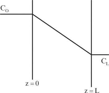
Figure 15-1 illustrates classic steady-state diffusion across a thin film at constant pressure and temperature with no convection in the direction of diffusion (z direction). At steady state there is no accumulation in the film, and the concentration profile does not change with time. This simple geometry can be used to experimentally determine diffusivity based on the definition derived from the Fickian model, Eq. (15-2b).
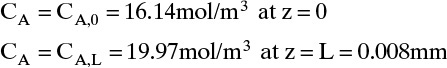
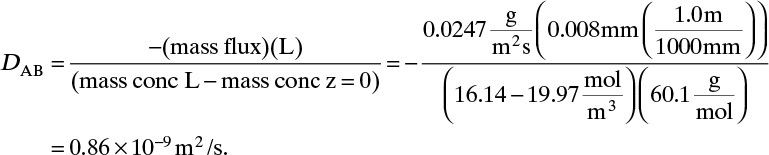
EXAMPLE 15-1. Determination of diffusivity in dilute binary mixture
To measure the diffusion coefficient of a dilute mixture of 1-propanol in liquid water at 25°C we set up a steady-state system in which the alcohol diffuses across a thin, flat liquid layer that contains a dilute alcohol-water solution. The water film is 0.008 mm thick, and the experiment is done with a 0.50 m × 0.40 m rectangle. We collect 0.382 g of 1-propanol in 1.289 minutes when concentrations are 19.97 mol/m3 (1.200 g/liter or 0.12 wt% at z = L and 16.14 mol/m3 at z = 0. Molecular weight of 1-propanol is 60.1 g/mol.
a. What is the diffusivity of 1-propanol in water at 25°C if the problem is solved in molar units?
b. What is the diffusivity of 1-propanol in water at 25°C if the problem is solved in mass units?
c. Determine the concentration profile of 1-propanol in the water film.
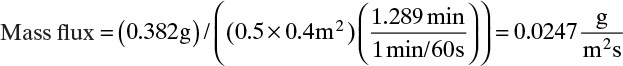
A. Since concentrations are low, convection is not important. We can calculate the molar flux, JA,z, from total amount transferred, area, and time interval:

The numerical value is

Next we need to integrate Eq. (15-4a) subject to boundary conditions:
For this example the numerical values are
For steady-state operation there is no accumulation of mass, and Eq. (15-4a) becomes

Separate variables in Eq. (15-6b) and integrate for constant DAB:
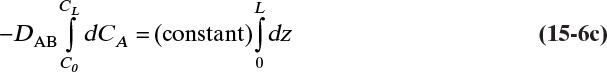
which becomes
Solving for DAB we obtain
From this equation the diffusivity is

This example illustrates that diffusion rates are quite low in liquid systems and that we must watch our units.
B. In this chapter we work consistently in terms of molar units. However, this restriction is not necessary. Because of an interesting property of the diffusion coefficient, the use of different units is straightforward. To illustrate, convert all terms in Example 15-1 to mass units:
Equation (15-4a) in mass units is

Following the same steps used to determine the diffusivity previously, we obtain
The calculated diffusivity is the same and has the same units! This is handy, since it says we can use the same diffusivity with any consistent flux and concentration units as long as the length and time dimensions are correct.
C. To determine the concentration profile, we can take the derivative of Eq. (15-4a), ![]() , with respect to z. For constant diffusivity,
, with respect to z. For constant diffusivity,

Integrating Eq. (15-8b) twice we obtain

Constants of integration K1 and K2 can be determined from boundary conditions, Eqs. (15-6a).
At z = 0, CA = K2 and thus K2 = CA,0.
At z = L, CA = CA,L = K1L +CA,0 which gives K1 = (CA,L – CA,0)/L
The resulting profile is linear:
To check this result, see if the equation satisfies the differential equation, Eq. (15-8b), and the boundary conditions. It does.
Example 15-1 is probably the simplest diffusion problem possible. Reread part C of this example noting the method used to determine the concentration profile. If data to determine flux, JA,z, had not been given, we would have substituted Eq. (15-8d) into Eq. (15-4a) and calculated the flux:

Note that with the problem defined with both concentrations and the diffusion length, L, given, the concentration profile does not depend on diffusivity, although the flux does depend on diffusivity. This result is not universal, and it is easy to pose problems in which the concentration profile does depend on diffusivity (e.g., Problem 15.D.1).
Equations very similar to Eqs. (15-8) and (15-9) occur in a number of situations, such as steady-state evaporation (Example 15-2) and steady-state permeation of gases and liquids in membranes.
EXAMPLE 15-2. Steady-state diffusion without convection: Low-temperature evaporation
Pure ethanol is contained at the bottom of a long, vertical tube (cross-sectional area = 0.9 cm2), as shown in Figure 15-2. Above the liquid is a quiescent layer of air. The liquid at the bottom of the tube is carefully adjusted so that distance from the air-liquid interface to the open top of the tube is constant at 15.0 cm. No liquid is withdrawn from the tube. At the open end of the tube air is blown perpendicular to the vertical tube so that the concentration of ethanol at the top of the tube is essentially zero. The entire apparatus is kept at 0°C, and ptot = 0.98 atm. The tube is carefully arranged so that there is no convection in the tube. Over the course of several days we find that the average evaporation rate is 0.9190 × 10⁻³ cm3/h. What is the value of the diffusion coefficient of ethanol in air at 0°C?
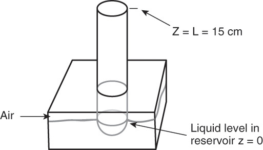
FIGURE 15-2. Tube and reservoir for Examples 15-2 and 15-3
Solution
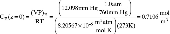
Liquid ethanol is evaporating at the bottom of the tube. If we assume equilibrium for the gas immediately above the liquid (z = 0), then
For an ideal gas C = yCm, where the total molar concentration of the gas is
Combining this result with Eq. (15-10a) for equilibrium evaporation, we obtain
The vapor pressure (VP) of ethanol can be accurately estimated by Antoine’s equation:

with VP in mm Hg, T in °C, A = 8.32109, B = 1718.10, and C = 237.52 over the range from –2 to 100°C (Dean, 1985). Note: Although mm Hg is an obsolete unit for pressure, because a large amount of data is in these units, engineers must be comfortable converting or using this unit.
The molecular diffusion coefficient can be determined from Eq. (15-9):
CL ≈ 0, C0 is given by Eq. (15-10c), and JA,Z can be determined from the evaporation rate:
Because evaporation rate is given in volumetric terms, we need a density. The molar density of liquid ethanol is 17,040 mol/m3. Once the ethanol flux is known, we can determine DAB.
Do it. Putting in numbers: At 0°C, VP = 12.098 mm Hg. Since the gas constant R = 8.20567 × 10⁻⁵ (atm m3)/(mol K),
Liquid evaporation rate,

Flux of ethanol in gas is
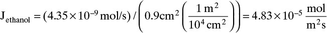
Then from Eq. (15-11a) we obtain

Comments
1. This result agrees with Table 15-1 in Section 15.3.
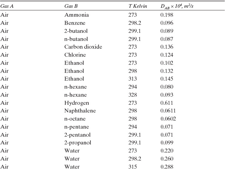
TABLE 15-1. Binary Fickian diffusivities for gases at 1.0 atm. For example, the diffusivity of air and ammonia at 273 K is 0.198 × 10⁻⁴ m2/s = 0.198 cm2/s. For each gas pair at low pressures and a given temperature, ptot DAB = constant*
*Cussler (2009); Demirel (2013); Geankoplis (2003); Poling et al. (2001, 2008); Sherwood et al. (1975); Treybal (1980)
2. Without significant horizontal convection in this problem, we would not be able to keep CL ≈ 0. However, this convection is not in the direction of diffusion, and since the system is dilute, convection induced in the z direction is quite small; thus Eqs. (15-6b) and (15-7) are valid. We are also assuming that air does not enter the tube or cause turbulent flow.
3. The most accurate method of measuring the amount of liquid that evaporates is to weigh the tube and the reservoir. Note that an operation with a reservoir and no liquid addition is not at a true steady state. However, if a large reservoir is attached to the tube bottom so that ΔL/L is small, the operation is almost at steady state (called pseudo-steady state), and steady-state diffusion equations can be used. See Problem 15.B1 to brainstorm alternative operating procedures.
4. The assumption that convection can be ignored is checked in Example 15-3.
15.2.3 Unsteady Binary Fickian Diffusion with No Convection (Optional)
We can also study unsteady diffusion in dilute systems. A classic unsteady-state diffusion problem is diffusion without convection in the direction of diffusion in an infinitely thick slab. The entire slab is initially at concentration Cinitial, and at t = 0 the z = 0 face of the slab is set to C = C0. At the far end of the slab, z → ∞, concentration is CA,∞ = Cinitial for all times; thus the slab is so thick that the far end is unaffected by diffusion. We will see shortly that with ordinary liquid diffusion coefficients, slabs do not need to be very thick to keep the far end at the initial concentration.
For a segment of thickness Δz, the mass balance per unit area is Accumulation = Input – Output. The amount of material in a segment of thickness Δz at any time t is CA(t) Δz. Since accumulation is the change in this amount of material, the mass balance becomes
Dividing by Δz and taking the limit as Δz → 0 (we need to assume this limit exists) we obtain
Since terms are now functions of both t and z, partial derivatives are required. Assuming constant diffusivity and substituting in Fick’s law, Eq. (15-4a), we obtain
This equation is often called Fick’s second law. Note that for steady state, Eq. (15-12c) becomes Eq. (15-8b). As expected, a very similar equation can be derived for unsteady-state heat conduction in an infinite slab (Incropera et al., 2011).
Boundary conditions for an infinitely thick slab are
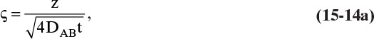
Defining the dimensionless distance ς (Greek letter zeta),
the solution for Eq. (15-12c) that satisfies the boundary conditions is
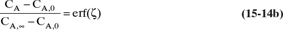
where erf is the error function. The definition and properties of the error function are discussed in Section 19.7.1 in conjunction with the solution for unsteady dispersion in adsorption columns. Since the error function is supported by Excel, calculations with a spreadsheet are straightforward. If CA,0 > CA,∞, a convenient form of Eq. (15-14b) for plotting results is
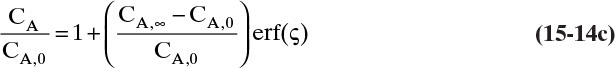
This equation was used to plot Figure 15-3 for diffusion of sucrose in liquid water.
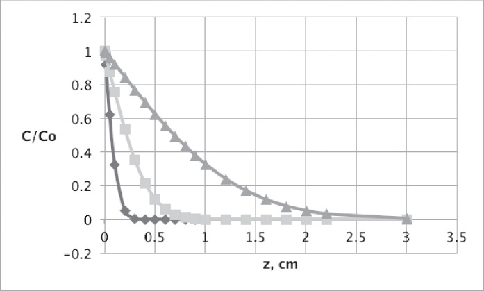
FIGURE 15-3. Unsteady diffusion of sucrose in an infinitely thick slab of water. Conditions are delineated in Problem 15.D19. Curves are C/Co and are plotted for t = 1000s ◊, 10,000s ![]() , and 100,000s Δ
, and 100,000s Δ
For different geometries it can be useful to write Fick’s second law in cylindrical coordinates for transfer in radial direction only:

and for spherical coordinates for transfer in radial direction only

Except for this section and Section 18.7 solutions of unsteady diffusion equations in one to three dimensions are beyond the scope of this book. Solutions to Eqs. (15-12c), (15-12d), and (15-12e), corresponding two- and three-dimension equations, and equivalent heat conduction equations have been extensively studied for a variety of boundary conditions (e.g., Crank, 1975; Cussler, 2009; Hines and Maddox, 1984; Incropera et al., 2011). Readers interested in unsteady-state diffusion problems should refer to these or other sources on diffusion. However, solutions to unsteady problems using a linear driving-force model are much more tractable and are analyzed in Sections 15.4.3 and 15.7.7.
15.2.4 Steady-State Binary Fickian Diffusion and Mass Balances with Convection
To simplify the previous analyses we assumed there was no convection in the z direction. In practical applications this is obviously a special case. How do we analyze diffusion with convection?
A useful analogy is to consider a sugar molecule moving in your body as you walk across a room. Overall movement of sugar will be dominated by your movement in the room (the room serves as a fixed frame of reference, and flux measured in this frame is N). To study the movement of the sugar, we first look at flux in your body using the body as the reference frame (meaning sugar movement is measured with respect to the body, not the room). Once we know flux J with respect to the moving reference frame, we can add flux J to the movement of your body to find N.
Since both convection and diffusion occur, we need to separate terms. In the Fickian model there are multiple correct methods to separate mass transfer into diffusion and convection terms. As a result, values of these two terms can be different if the calculation is done in different, yet correct, ways. However, the final answer, the total amount of mass transferred, will be the same. The usual assumption is that we can find a reference frame with diffusion and no convection. The diffusion problem is then solved in this reference frame. Then we add the effects of convection in a fixed reference frame to obtain the total flux, NA mol/(m2s).


This step certainly makes sense in the analogy with your body. Fick’s law is applied in a reference frame (your body) with no convection, which allows use of the procedures of Section 15.2.2. Since we are doing a steady-state analysis the total fluxes, NA and NB [mol/(m2s)] are constant (e.g., not functions of z); however, the diffusive and convective fluxes may depend on z. To use this separation of terms, choose a reference velocity vref (z) so that there is no convection in the reference frame. This is always possible in a steady-state system. The convective flux is defined in terms of the reference or basis velocity vref times the molar concentrations.
where CA and CB are in mol/m3 and vref is in m/s. Since vref, CA, and CB can depend on z, the convective fluxes can depend on z.
The total flux of components A and B (due to both diffusion and convection) can be defined in terms of currently unknown component transfer velocities vA(z) and vB(z):
The diffusive flux of A is given by Eq. (15-4a), since it is calculated in a reference frame with no convection, and there is a similar equation for B. The diffusive flux of A can also be determined by subtracting Eq. (15-15c) from (15-15e) because JA is the difference between the total flux and the convective flux (in the analogy, this step allows us to look at only what is happening within your body). Comparing the diffusive flux found from Eqs. (15-15c) and (15-15e) with the result from Eq. (15-4a), we have
In a similar fashion we obtain
Solving for the component transfer velocities,
If we expand Eqs. (15-15e) and (15-15f)
NA = CA vA = CA(vA – vref) + CA vref
NB = CB vB = CB(vB – vref) + CB vref
and combine the expanded terms with Eqs. (15-16a) and (15-16b), we obtain the total fluxes:
To find the total fluxes we have to decide on an appropriate reference coordinate system and reference or basis velocity. Because the reference coordinate system is defined as a system in which there is no convection, the net flux of A plus B must be zero; otherwise there would be convection. Thus in the reference coordinate system moving at reference velocity vref, by definition,
If we add Eqs. (15-16e) and (15-16f), apply Eq. (15-17a) to remove the diffusivity terms, and note that mole fractions in a binary gas system are
(Cm is total molar concentration [e.g., kmol/m3]). The molar reference velocity is
In a liquid system replace the symbol y with x. If we want to calculate a mass flux while retaining the molar reference velocity, we can multiply Eqs. (15-16e) and (15-16f) by MWA and MWB, respectively.
Following steps similar to those used to derive the molar reference velocity, we can develop the mass reference velocity:
For a volumetric flux divide Eqs. (15-16e) and (15-16f) by the molar densities of A and B, respectively, and proceed with the same steps in the derivation to develop the volumetric reference velocity:
Remembering that fractions are defined so that
Eq. (15-17c1) can be written in terms of the molar fluxes:
There are similar equations for vref,vol and vref,mass. Note that reference velocities vref,vol, vref,mol, and vref,mass can be identical or different depending on whether volume, mole, or mass fractions are the same. For example, volume and mole fractions are identical in an ideal gas, and vref,vol = vref,mol. If the molecular weights are different, vref,mol ≠ vref,mass. Why have we introduced three reference velocities? And how do we decide which reference velocity vref should be used?
Use the reference velocity that makes the problem as simple as possible! The choice of reference velocity and the solution of Fickian diffusion problems are best illustrated with examples. A reference velocity of zero is often a good choice; however, in the analogy with your body the reference velocity was not zero, but the solution was not difficult. In this analogy we would probably use mass fractions, with A as the sugar and B as everything else, to calculate vref,mass. Since there is a lot more mass of the body than mass of the sugar, xB,ref = xBody,wt frac >> xA,ref = xsugar,wt frac, xB,ref ∼ 1, and vref,mass ∼ vBody,mass. So to find the total flux of sugar, we add the velocity at which you walk across the room to the diffusive flux of sugar within your body. We could use vref,vol in this analogy with your body, but mass is more familiar.
For a second example assume we have two fixed, equal-volume chambers (Figure 15-4) that contain different ideal gases but are at the same pressure and temperature. With ideal gases at constant pressure and temperature, there is no volume change on mixing. Since JA = –JB, there will be equal and opposite molar flows of gases A and B, and the molar reference velocity vref,mol = 0. This case is an example of equimolar counter diffusion, which obviously simplifies the equations. Equations (15-16e) and (15-16f) become
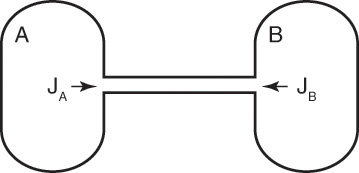
FIGURE 15-4. Counter diffusion of ideal gases. Chambers have equal volumes, pressures, and temperatures
Use of a volume average reference velocity also results in vref,vol = 0, but if molecular weights are different, a mass average reference velocity will not be zero. Even if the gas is not ideal, the use of molar or volumetric reference velocities will often make an approximate solution easier.
Calculation of diffusion in distillation columns tends to be easier if the molar average reference velocity vref,mol is used. In distillation, constant molal overflow is often valid or close to valid (Section 4.2). The resulting equimolar counter diffusion results in NA = –NB, and there is no convection in the reference frame with vref,mol = 0. If we choose the reference velocity as molar average velocity, the result is Eq. (15-18). A similar simplification occurs for linear driving force analysis in Section 15.4 and for analysis of distillation in Section 16.1.
A third example that frequently occurs in evaporation, absorption, and stripping is binary diffusion through a stagnant fluid. In this case NB = 0. Setting NB = 0 in Eq. (15-17d), we find vref,mol = NA/Cm. Substitution of this result into Eq. (15-16e), defining gas mole fraction yA = CA/Cm, and solving for NA, we obtain the flux equation for A:
This result is derived in a different way in Example 15-3.
Most liquids have no or very little volume change on mixing—one of the ways to estimate the density of a liquid mixture is to assume volumes are additive. Even liquid systems with large volume changes on mixing rarely have more than a 10% change. Molar and mass densities are usually significantly less constant. In this case the volumetric reference velocity vref,vol is the simplest reference velocity to use.
In separations it is common to use vref,mol for distillation and absorption, vref,mass for extraction, and vref,vol for gas permeation through membranes. In fluid dynamics the mass average velocity is usually chosen as the reference velocity. On the other hand, Cussler (2009) states that use of the volumetric average velocity vref,vol often results in the simplest diffusion problem.
Diffusion problems are almost always solved as special cases. These solutions are tabulated in significant detail in Crank (1975), Cussler (2009), Hines and Maddox (1984), and Incropera et al. (2011). Example 15-3 presents the special case of steady-state diffusion of component A through a stagnant layer of B. This case is important for evaporation, absorption, and stripping.
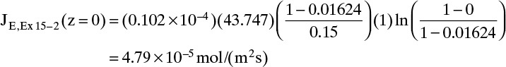
EXAMPLE 15-3. Steady-state diffusion with convection: High-temperature evaporation
Repeat Example 15-2 (Figure 15-2), but operate at a temperature of 39.85°C = 313 K, use the diffusivity value from Table 15-1 (Section 15.3.1), and calculate both diffusion flux JEthanol and total flux NEthanol at z = L and at z = 0.
Solution
A. Define. We are to calculate diffusion flux of ethanol at z = 0 and at z = L and calculate the flux of ethanol for the system shown in Figure 15-2 at 313 K. In addition we will determine if convection was important in Example 15-2.
B, C. Explore and Plan. With a higher temperature the VP will be significantly higher, and the concentration C0 given by Eq. (15-10b) will be higher. Thus convection effects are much more likely to be significant. Since operation is at steady state, NA is constant and is not a function of either time or distance in the tube. Because air (component B) is stagnant, NB = 0 and vB = 0. The molar average reference velocity, Eq. (15-17b1), simplifies to
We will see shortly that vref,mol is constant but not zero. In a reference frame moving at velocity vref,mol, convective flux is zero. Substituting Eq. (15-19a) into (15-16e),

We used NA = CAvA for the last equals sign. Solving for NA and substituting in CA = CmyA,mol,

This result is the same as Eq. (15-18c). Rearranging this equation and integrating, we have for constant flux NA
For an ideal gas Cm = ptot/(RT), and volumetric and molar fractions are equal. Thus
and Eqs. (15-19a) to (15-19d) are also valid for volume reference velocity and volume fractions. The gas constant R = 8.20567 × 10⁻⁵ (atm m3)/(mol K). Note that
NA = CAvA =CmyA,molvA = (ptot/RT)yA,molvA = constant
Since pressure and temperature are constant, Cm is constant and product of yA,mol × vA = constant, which from Eq. (15-19a) makes vref,mol constant. We will also assume that DAB is constant—as shown later in Example 15-5 diffusivities are often not constant.
The boundary condition at z = L is CA = CA,L ≈ 0, which is
At z = 0, CA = CA,0, which from Eq. (15-10c) is CA,0 = VP(T)/(RT)
The solution to Eq. (15-19d) for constant diffusivity is (Cussler, 2009)

For the boundary conditions of our example the constant flux NA is

The concentration decreases from z = 0 to z = L:
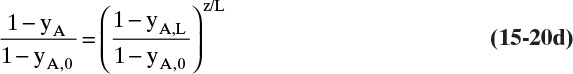
Note that this equation satisfies the boundary conditions. The total flux is constant, but since the concentration profile is not linear, the diffusion flux depends on distance z.

Since by definition JA = –JB in the moving reference frame, we have

but in the stationary reference frame NB = 0.
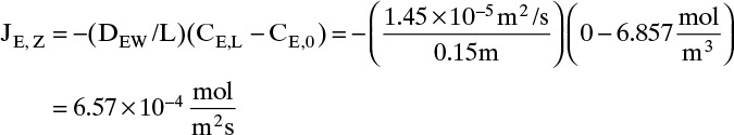
D. Do it. Putting in the numbers: From Antoine’s equation (Example 15-2), VPEthanol = 133.85 mm Hg. Concentration of ethanol in the gas next to the liquid surface is Csurface = 6.857 mol/m3. yEthanol,0 = VP/ptotal = 0.1797, and yEthanol,L = 0. From Table 15-1, DEthanol-air = 0.145 × 10⁻⁴ m2/s. The total concentration Cm is
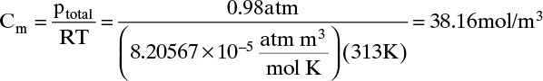
Note that, as expected, at z = 0, Csurface = yethanol,0Cm. From Eq. (15-20f) at z = L = 0.15 m and at z = 0,
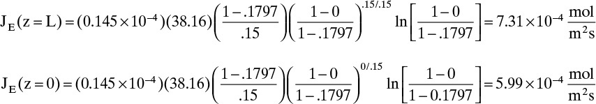
The total flux rate:

At z = L, where yA = 0, Eq. (15-20a) requires diffusion flux and the total flux to become equal. The numerical values satisfy this constraint.
E. Check on Example 15-2. Since the convective flux in Example 15-3 was largest at z = 0, we will check if the convective flux is significant at z = 0 in Example 15-2, which neglected convection. The convective flux is
Convective flux (z = 0) = NE – JE(z = 0)
Using the values from Example 15-2, we have
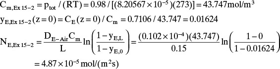
At z = 0, Eq. (15-20f) becomes
Finally, the convective flux in Example 15-2 is
Convective flux (z = 0) = NE – JE(z = 0) = 0.08 × 10⁻⁵ mol/(m2s)
Thus even at z = 0, where the convective flux is highest, it is only 1.6% of the total flux. When the convective flux is neglected, NE = JE, which was calculated as 4.83 × 10⁻⁵. This is an error of 0.8% in the total flux. Thus neglecting the convective flux in Example 15-2 is valid.
Neglecting flux in Example 15-3. Suppose we had neglected the flux in Example 15-3. Then the solution for JE,z would be obtained from Eq. (15-9). With the ethanol concentration at z = 0 and the ethanol diffusivity of Example 15-3, this is
Since we are neglecting convection, we would set the total flux to NE = JE. Since the actual total flux was 7.31 × 10⁻⁴, the error would be 10%, and neglecting the convective flux in Example 15-3 is not valid. The error is larger for higher temperatures.
F. Generalization. If NB = 0 and Cm is constant, then Eq. (15-19c) is a general result. It is applicable for liquids by replacing y with x. If Cm is constant, then vref is also constant. If the boundary conditions are
yA (z = L) = yA,L and yA (z = 0) = yA,0 [or xA (z = L) = xA,L and xA (z = 0) = xA,0]
then the solution is given by Eqs. (15-20a), (15-20b), and (15-20d) to (15-20f) regardless of the method used to determine the values of yA,L and yA,0 [or xA,L and xA,0]. Thus this result can be applied to other physical situations.
Students often find this section confusing. The choice of reference velocity based on volume, mole, or mass appears arbitrary and may result in different values for convective flux. This in turn results in different values for diffusive flux. Even though total fluxes of A and B do not change, how is this correct? In physical situations there is only total flux. Separating this flux into convective and diffusive terms is a human invention. The method works because diffusive flux is defined with respect to a reference frame in which convective flux is zero. If we change vref, we change convective and diffusive fluxes by the exact amounts required to keep total fluxes unchanged. If we report diffusive flux and convective flux, we need to be clear whether a volume, mole, or mass basis was used. Another way to think about this calculation is total fluxes of A and B are state functions—they do not depend on the calculation path chosen. Diffusive and convective fluxes are path functions and depend on how the calculations are done.
15.3 Values and Correlations for Fickian Binary Diffusivities
As noted earlier determination of diffusivity requires that a model be defined so that the concentration data can be analyzed. Almost all diffusivity data tabulated in the literature (e.g., Cussler, 2009; Demirel, 2013; Marrero and Mason, 1972; Poling et al., 2001, 2008; Sherwood et al., 1975) were analyzed with the Fickian model.
15.3.1 Fickian Binary Gas Diffusivities
Based on the molecular argument in Section 15.1 we expect that diffusivities will increase with increasing temperature. This is indeed the case. Fortunately in most cases temperature dependence can be quite accurately predicted. Ideally diffusivity would not depend on concentration. For gases this is approximately true. Typical diffusivity data for gases are given in Table 15-1. At pressures below about 70 atm and at a constant temperature, the product [ptot DAB] is constant for each gas pair, and DAB is independent of concentration.
Please do not consider the tables as an opportunity for a reading break. Instead of skipping Table 15-1, study the numbers and search for patterns. Obviously DAB increases as temperature increases. By comparing data for different alcohols in air at 298 K the pattern that emerges is DAB values are larger for molecules with lower molecular weights. This is generally true even for very different molecules if there is a big difference in molecular weights.
Diffusivities for gas pairs can be fairly accurately predicted from kinetic theories. A simple kinetic theory for hard spheres predicts (Cussler, 2009):
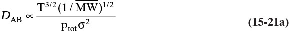
T is absolute temperature in Kelvin, ![]() is an average molecular weight, ptot is total absolute pressure in atmospheres, and σ is average diameter of the spherical molecules in Å.
is an average molecular weight, ptot is total absolute pressure in atmospheres, and σ is average diameter of the spherical molecules in Å.
The more detailed and accurate Chapman-Enskog kinetic theory is valid for nonpolar molecules to about 70 atm. This equation with DAB in m2/s (Cussler, 2009; Geankoplis, 2003; Sherwood et al., 1975; Wankat and Knaebel, 2008) is

The collision diameter σAB is determined from the Lennard-Jones potential parameters,
and dimensionless ΩD is a collision integral that is a function of kBT/εAB, where kB is Boltzmann’s constant (1.38066 × 10⁻²³ J/K) and εAB is the Lennard-Jones energy of interaction, which can be calculated from values for the two molecules:
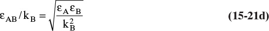
Table 15-2 is a brief list of Lennard-Jones parameters and values of ΩD. Detailed tables are available for a variety of compounds to calculate these parameters (e.g., Cussler, 2009; Hirschfelder et al., 1964). An empirical fit for ΩD is given in Eq. (15-21e) (Wankat and Knaebel, 2008):
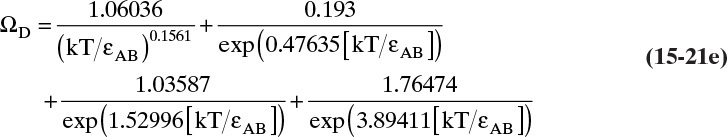
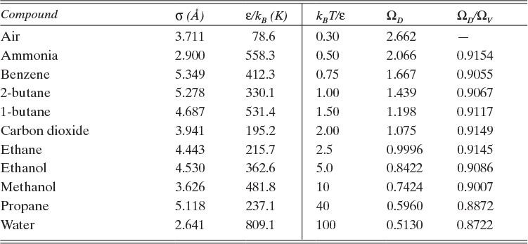
Sources: Cussler (2009); Hirschfelder et al. (1964); Sherwood et al. (1975)
TABLE 15-2. Lennard-Jones potential parameters (left side of table) and values of the collision integrals (right side of table) for ideal Fickian gas diffusivity calculation with the Chapman-Enskog equation (15-21)
Because the collision integral is temperature dependent, gas diffusivities are proportional to T2 at low temperatures and to T1.66 at high temperatures. Wankat and Knaebel (2008) summarize other methods to predict gas diffusivities.
The kinetic theory of gases can also be used to predict the dimensionless Schmidt number, ScV = µ/(ρDAB), which is useful because the Schmidt number is used in correlations for the mass transfer coefficient (see Section 15.5). For diffusion of component A at low concentrations in gas B, ScV can be estimated from (Sherwood et al, 1975)

ΩV is the viscosity collision integral. Values of ΩD/ΩV given in Table 15-2 can be calculated from kBεB/T.
Although prediction methods are available, it is always better to have an experimental value for DAB and then adjust for pressure or temperature differences. Equations (15-21a) and (15-21b) predict the same inverse dependence of diffusivity on pressure but a slightly different dependence on temperature. If a single experimental value is available, DAB can be accurately predicted at any temperature or pressure. This is illustrated in Example 15-4.
EXAMPLE 15-4. Estimation of temperature effect on Fickian gas diffusivity
Estimate the diffusivity of carbon dioxide in air at 317.3 K and 1.0 atm.
Solution
From Table 15-1 Dair–CO2 = 0.136 × 10⁻⁴ m2/s at 273 K and 1.0 atm. From Eq. (15-21a)

From Eq. (15-22b), at low temperatures the temperature exponent is approximately 2.0,

From Eq. (15-22b), at high temperatures the temperature exponent is approximately 1.66,

The experimental value is 0.177 × 10⁻⁴ m2/s. Predicted value with an exponent of 3/2 is 4.0% low, predicted value with an exponent of 2.0 is 4.0% high, and predicted value with an exponent of 1.66 is 1.1% low.
15.3.2 Fickian Binary Liquid Diffusivities
Experimental binary diffusivity data for liquid systems are presented in Table 15-3. As temperature increases (compare chlorobenzene-bromobenzene data at same concentrations or infinite dilution ethanol-water data), diffusivity increases. Pressure is not expected to affect liquid diffusivities. Data for proteins in Table 15-3 show that, as expected, diffusivities are significantly lower than for low molecular weight compounds, and diffusivity decreases as molecular weight of the protein increases. Diffusivities (shown for sucrose) decrease in aqueous gels as more solid is added and the gel becomes more viscous. Most tabulations of liquid diffusivity data in the literature give values at infinite dilution limits or for just a few concentrations. Compare the infinite dilution value for ethanol in water to the value for water in ethanol. In general, ![]() (see Problem 15.A3).
(see Problem 15.A3).
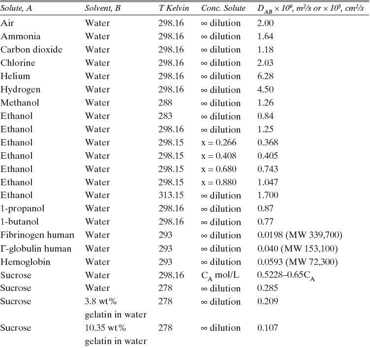
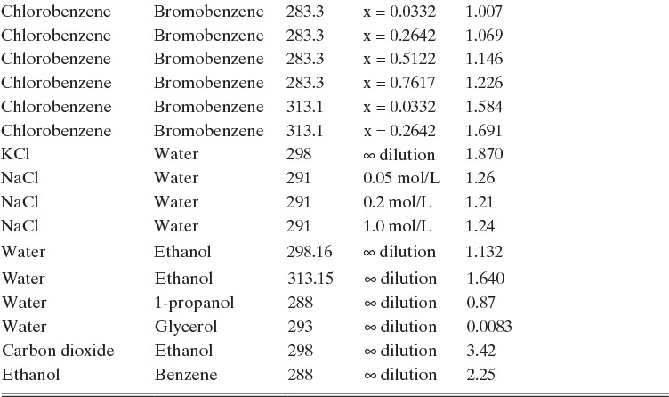
TABLE 15-3. Binary Fickian diffusivities for liquids. For example, the diffusivity of air in water at 298.16 K is 2.00 × 10⁻⁹ m2/s = 2.00 × 10⁻⁵ cm2/s.* x is mole fraction of solute A
*Cussler (2009); Demirel (2013); Geankoplis (2003); Poling et al. (2008); Sherwood et al. (1975); Treybal (1980); Tyn and Calus (1975)
There are a number of theories for predicting diffusivity of liquids at infinite dilution (Cussler, 2009; Kirwan, 1987; Poling et al., 2001; Sherwood et al., 1975; Wankat and Knaebel, 2008). Many of these theories use the Stokes-Einstein equation as a starting point (Bird et al., 2006; Cussler, 2009; Wankat and Knaebel, 2008).
In this equation µB is solvent viscosity, and ![]() is the solute radius, which is assumed to be a rigid sphere with gravity as the only body force. The Stokes-Einstein equation works best for unhydrated molecules with a molecular weight greater than 1000, and even there it is not very accurate.
is the solute radius, which is assumed to be a rigid sphere with gravity as the only body force. The Stokes-Einstein equation works best for unhydrated molecules with a molecular weight greater than 1000, and even there it is not very accurate.
The most popular theory for diffusivity of liquids is Wilke-Chang theory (Cussler, 2009; Sherwood et al., 1975; Wankat and Knaebel, 2008), which uses the Stokes-Einstein equation as a starting point and predicts infinite dilution diffusivity of solute A in solvent B, ![]() .
.

In this equation VA is molar volume of solute in m3/kmol at its normal boiling point, T is in Kelvin, solvent viscosity µB is in Pa • s [kg/(m s)], φB is a solvent interaction parameter, and D°AB is in m2/s. There is some disagreement in the literature on appropriate values of φB, particularly for water. The following values are recommended for different solvents (Wankat and Knaebel, 2008): water, φB = 2.26 (other authors such as Geankoplis [2003] recommend φB = 2.6); methanol, φB = 1.9; ethanol, φB = 1.5; propanol, φB = 1.2; other solvents, φB = 1.0.
Although not obvious from the Wilke-Chang equation’s form, because of variation of viscosity with temperature, it predicts an Arrhenius dependence on temperature (Kirwan, 1987):
Typical values for the activation energy Eo are approximately 10,000 J/mol and R = 8.314 J/(mol K). This equation can also be used at constant mole fractions instead of infinite dilution if data are available (see Problem 15.D5). Alternatively, if the effect of temperature on solvent viscosity is known, we can write Eq. (15-22b) for both temperatures and take the ratio of these equations:

In more concentrated solutions Eq. (15-22d) becomes

which although not exact is still useful.
Unfortunately, except in quite dilute mixtures, liquid diffusivity is rarely constant, and very large changes in DAB are often observed going from a trace of A in almost pure B (infinite dilution limit) to a trace of B in almost pure A (other infinite dilution limit). For example, compare the change in DAB in Table 15-3 for a relatively ideal chlorobenzene–bromobenzene system at 283.3 K to the change in DAB for a nonideal ethanol–water system at 298.15 K. The former values increase modestly, while the latter values go through a minimum as water mole fraction increases.
If the diffusivity is not constant, we would at least hope that there is a relatively simple relationship that allows calculation of DAB at any concentration based on the two infinite dilution limits, ![]() and
and ![]() . The Vignes correlation based on the activity coefficient γA is reasonably accurate (Kirwan, 1987; Sherwood et al., 1975; Treybal, 1980) for moderately nonideal systems:
. The Vignes correlation based on the activity coefficient γA is reasonably accurate (Kirwan, 1987; Sherwood et al., 1975; Treybal, 1980) for moderately nonideal systems:

The last term is a thermodynamic correction factor for nonideal solutions. Equation (15-22f) predicts that DAB is not constant even for ideal systems [term in brackets in Eq. (15-22f) has a value of 1.0]. Equation (15-22f) can also predict a negative diffusion coefficient, which is an indication of the formation of two liquid phases.
The most accurate results are obtained not by predicting diffusivity but by obtaining experimental values at two, preferably more, temperatures and then adjusting for temperature differences. Activity coefficient data is required to adjust for concentration changes in nonideal systems.
15.3.3 Numerical Solution with Variable Binary Diffusivity
In dilute systems at constant pressure and temperature we can often assume DAB and Cm do not depend on concentration. In ideal gas systems DAB and Cm are functions of temperature and pressure, and in nonideal gases DAB and Cm are also often functions of molar concentration, although variation in DAB is often small. In liquid systems DAB and Cm are typically functions of temperature and concentration, and concentration effects may be quite significant.
For systems at constant temperature and pressure, only the concentration effects on diffusivity need to be considered. In addition, total molar density Cm can be a function of concentration. The effects of concentration on diffusivity in liquid systems are considered in detail in section 15.3.2. In this section we assume that experimental values of diffusivity are available. A simple numerical solution method for steady-state diffusion problems with convection when DAB and Cm depend on concentration is illustrated.
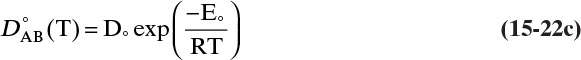
EXAMPLE 15-5. Numerical solution for variable diffusivity and molar concentration
A steady-state system of ethanol and water has equal molar counter diffusion across a liquid film of thickness 1.2 × 10⁻⁵m. At z = 0 the ethanol mole fraction is 0.010 and at z = L the ethanol mole fraction is 0.300. Operation is at 40°C. Find the flux of ethanol.
Simple But Incorrect Solution
A. Define. Find the flux of ethanol.
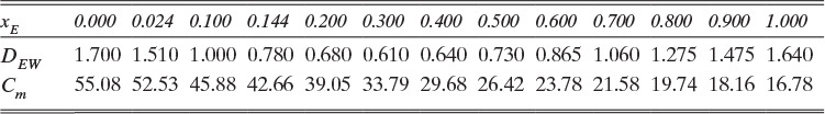
B. Explore. Table 15-3 lists the diffusivity of ethanol in water at 40°C (313.15 K) at infinite dilution as DEW (xE →0) = 1.700 × 10⁻⁹ m2/s, and diffusivity of water in ethanol at 40°C (313.15 K) at infinite dilution as DWE (xW →0) = 1.640 × 10⁻⁹ m2/s. Infinite dilution data appears to confirm that the use of constant DEW = 1.700 × 10⁻⁹ m2/s would be quite accurate. Pure water at 40°C has molar concentration Cm = 55.08 kmol/m3.
C. Plan. Assume diffusivity and total molar concentration are constant. Calculate flux using these values to integrate Eq. (15-18).
D. Do It.
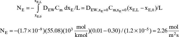
E. Check. If no other data were available that showed diffusivity and total molar concentration are not constant, we would be tempted to believe this value. However, since ethanol and water is commercially very significant, it has been very extensively studied. Table 15-4 presents extensive diffusivity and molar concentration data for this system. DEW and Cm are not constant, and they are both at their highest values at xE = 0. Thus predicted flux is obviously too high. Since diffusivity and molar concentration vary, we need to integrate numerically.
Sources: Tyn and Calus (1975); Perry and Green (p. 2-117, 2008)
TABLE 15-4. Fickian diffusivity of the system ethanol-water at 40°C (all diffusivities × 10–9 m2/s). Mole fraction of ethanol is xE. The Cm values in kmol/m3 were added to the chart and are based on the liquid densities of ethanol-water mixtures
Revised Solution
We need to integrate Eq. (15-18), NE = –DEWdCE/dz = –DEWCmdxE/dz, subject to the boundary conditions
xE = xE,0 = 0.010 at z = 0 and zE = xE,L = 0.30 at z = L
with nonconstant DEW and Cm. Since the system is at steady state, NE = constant. Separating variables and integrating, we obtain
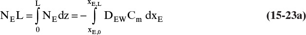
The integral on the right-hand side needs to be evaluated numerically. There are a number of ways to do this. A reasonably accurate approach when the integrand is monotonic is to use Simpson’s rule, Eq. (9-12), which for this integration is
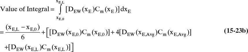
where xE,Avg = (xE,0 + xE,L)/2 = (0.01 + 0.30)/2 = 0.155.
The values of DEW and Cm at are given in Table 15-4. The values at xE,0 = 0.010 and xE,Avg = 0.155 can be estimated by linear interpolation. For example, at xE,0 = 0.010 we have
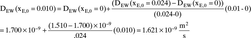
The corresponding other values are
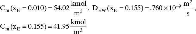
Value Integral = (0.29/6)[(1.621)(54.02) + 4(0.76)(41.95) + (0.61)(33.79)] × 10–9 = 11.392 × 10⁻⁶
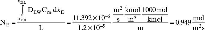
More accuracy for the numerical integration can be obtained by dividing the concentration range into several parts and integrating each part with Simpson’s rule. This procedure can be automated in a spread sheet by using Lookup Tables and linear interpolation for the tabular data. The result with two areas is NE = 0.973 mol/(m2s), which is 2.5% higher than the result with a single area for the calculation.
Note that the estimate done initially with DEW and Cm calculated at xE = 0 was off by more than a factor of two.
15.4 Linear Driving-Force Model of Mass Transfer for Binary Systems
Unfortunately, because of the complexity of geometry and flow fields in most separators, reactors, and other devices in which interfacial mass transfer occurs, solution of diffusion equations is not usually feasible. In these cases we typically use the empirical linear driving-force model for mass transfer that is briefly introduced in Section 1.3. This equation [a modification of Eq. (1-4)] is
As noted in Section 15.1, the use of driving force can be misleading, since the molecules have no brain or intention to transfer, and in molecular diffusion processes transfer occurs because of random collisions. However, since driving force is embedded in the jargon of chemical engineering, we use the term here. The strength of Eq. (15-24a) is that it is very broad and flexible and can be applied to a wide variety of situations. The weakness of this equation is that it is empirical, and its theoretical background is based on film theory (Section 15.4.1), which is not always applicable. In some practical situations a few experiments will suffice to provide the mass transfer coefficient in the range of interest. If temperature, pressure, and concentrations vary significantly in the separator, successful application of Eq. (15-24a) requires a correlation for the mass transfer coefficient based on extensive experimental data.
Equation (15-24a) can be written in terms of concentrations as
If the flux is desired in (kmol A)/(s m2), the area across which the mass transfer occurs is measured in m2, and concentration is in (kmol A)/m3, then the mass transfer coefficient kc has units of velocity, m/s. In single-phase systems the concentrations CA,2 and CA,1 are the (kmol A)/m3 at locations 1 and 2, which are usually the system boundaries. For mass transfer from one phase to another, one of the concentrations would be the concentration at the interface. Typical values for the mass transfer coefficient are 0.1 m/s for gases and 10–4 m/s for liquids (Wesselingh and Krishna, 2000).
We can also write the mass transfer equation in terms of liquid mole fractions:
In terms of vapor mole fractions the equation is
In these cases mass transfer coefficients kx and ky have units (kmol A)/[m2 s (mole fraction A)] or equivalently (kmol fluid mixture)/(m2 s). Occasionally, flux is written in terms of a partial pressure driving force, pA = yAptot,
In this case mass transfer coefficient kp = ky/ptot has units (kmol fluid mixture)/(m2 s bar).
In Section 15.2.1 the analogy between heat and mass transfer was discussed. This analogy also extends to linear driving force models as long as heat transfer by radiation can be neglected. The heat-transfer equation analogous to Eq. (15-24a) is
The heat-transfer equation analogous to Eqs. (15-24b) to (15-24e) is
Here Qz/A is the heat flux in J/(m2s), hheat transfer is the heat-transfer coefficient in J/(m2s • K), and T2 and T1 are temperatures at the two system boundaries, K. The analogy between heat and mass transfer will prove useful in determining correlations for the mass- and heat-transfer coefficients in Section 15.5.4.
15.4.1 Film Theory for Dilute and Equimolar Transfer Systems
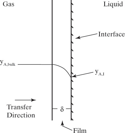
Figure 15-1 shows diffusion across a thin layer or film. Later in this chapter Figure 15-5 shows mass transfer to an interface through thin films of gas and liquid. After that Figure 15-6 shows mass transfer in absorption when the liquid mass transfer rate is very rapid, and Figure 15-8 shows mass transfer to a falling liquid film. The reason for this interest in mass transfer through films is that the most commonly used model for mass transfer in separators is a film model. The film model assumes that mass transfer to a surface or interface from bulk fluid occurs across a stagnant film of unknown thickness Δ. The mass transfer rate in this film occurs by molecular diffusion alone and can be modeled with Fick’s law, the Maxwell-Stefan analysis, or one of the forms of Eq. (15-24). In Section 15.2 we saw that flux JA is the flux in a reference coordinate system moving at a reference velocity vref that made JA = –JB so that net flux in the reference coordinate system was zero. However, we really want flux NA calculated with respect to fixed equipment coordinates. In this section we develop film theory for dilute systems and systems with equimolar counter transfer, both of which have NA = JA. These systems are important for dilute absorbers and extractors and for distillation, which is usually very close to equimolar counter transfer.
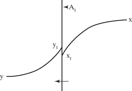
Since film theory postulates that mass transfer occurs across a stagnant film, we can use the Fickian diffusion solution from Eq. (15-9) for diffusion across a thin layer of fluid. If this thin layer is a gas film of unknown thickness Δ and we convert from concentrations to mole fractions, we obtain
For systems that are dilute or have equimolar counter transfer NA,z = JA,z. Since film thickness Δgas is unknown, the mass transfer coefficients kc,gas and ky are defined as
Then the equation for mass transfer for dilute or equimolar counter transfer is
Because it uses the Fickian diffusion solution for diffusion across thin layers to define the mass transfer equations and mass transfer coefficients, the linear driving-force model has Fickian genes. Thus the linear driving-force model inherits the good traits (e.g., simplicity, analogous to heat transfer, works well for binary systems, vast quantities of data) and the bad traits (nonideal diffusivities are difficult to predict, theory does not extend easily to multicomponent systems, see Section 15-6) of Fickian diffusion.
For equilibrium staged and sorption separations, we are interested in mass transfer from one phase to another. This is illustrated schematically in Figure 15-5 for transfer of component A from the liquid to the vapor phase. xA,I and yA,I are interfacial mole fractions. For dilute absorbers and strippers and for distillation where there is equimolar counter transfer, mass transfer Eqs. (15-26d) and (15-26e) can be written for each stage in the following different forms:
or
where ky and kx are the individual mass transfer coefficients with mole fraction driving forces for vapor and liquid phases, respectively, and kc,gas and kc,liq are the individual mass transfer coefficients with concentration driving forces for vapor and liquid phases, respectively. At steady state the rates of mass transfer in the gas and liquid phases have to be equal, and NA,z,gas = NA,z,liq. Additionally, the assumption is usually made that the gas and liquid at the interface are in equilibrium. If there is a resistance to obtaining equilibrium at the interface (e.g., if a surface-active agent is present), then an equation for this resistance must be included.
Unfortunately, there are two major problems with these equations when they are applied to vapor-liquid and liquid-liquid contactors. First, the interfacial area AI between the two phases is very difficult to measure. This problem is usually avoided by writing Eqs. (15-27) as
where a is the interfacial area per unit volume (m2/m3). Since a is no easier to measure than AI, we often measure and correlate the products kya, kxa, kc,vapa, and kc,liqa. Typical units for kya and kxa are kmol/(s m3) or lbmol/(h ft3), and for kca typical units are [(m/s)(m2/m3)] = s–1.
The second problem is that the interfacial mole fractions are also very difficult to measure. To avoid this problem, mass transfer calculations often use a driving force defined in terms of hypothetical equilibrium mole fractions.
These equations, which are a repeat of Eqs. (1-5), define the overall mass transfer coefficients Ky and Kx. Typical units for Kya and Kxa are kmol/(s m3) and lbmol/(h ft3). ![]() is the vapor mole fraction, which would be in equilibrium with the bulk liquid of mole fraction xA, and
is the vapor mole fraction, which would be in equilibrium with the bulk liquid of mole fraction xA, and ![]() is the liquid mole fraction that would be in equilibrium with the bulk vapor of mole fraction yA.
is the liquid mole fraction that would be in equilibrium with the bulk vapor of mole fraction yA.
To obtain the relationship between the overall and individual coefficients, we begin by assuming there is no resistance to mass transfer at the interface. This assumption implies that xI and yI must be in equilibrium. The mole fraction difference in Eq. (15-29a) can be written as
where m is the average slope of the equilibrium curve (yA versus xA) at xA and xAi.
Combining Eq. (15-30a) with Eqs. (15-28) and (15-29a), we obtain
which leads to the result
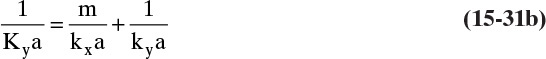
Similar manipulations starting with Eq. (15-29b) lead to
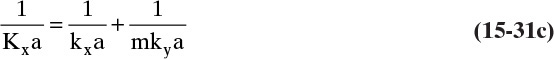
If there is a resistance at the interface, then this resistance must be added to Eqs. (15-31a), (15-31b), and (15-31c). This sum-of-resistances model shows that the overall coefficients will not be constant, even if kx and ky are constant, if the equilibrium is curved and m varies. In binary distillation m is the tangent to the equilibrium curve at xA,avg = (xA,I + xA)/2, and since the equilibrium curve is never straight, m has to vary. For example, if we have a constant relative volatility system with equilibrium given by Eq. (2-22b), m from Eq. (15-30b) is
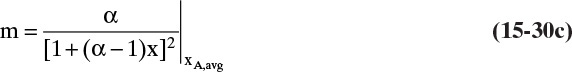
As an example of the variation in m, if the relative volatility α = 2.5, at xA,avg = 0.01, m = 2.43; at xA,avg = 0.5, m = 0.82; and at xA,avg = 0.99, m = 0.40. At the very least, average values of m need to be determined separately for the stripping and enriching sections.
Equations (15-31a), (15-31b), and (15-31c) also show the effect of equilibrium on the controlling resistance. If m is small, then from Eq. (15-31b) Ky ∼ ky and the gas-phase resistance controls. If m is large, then Eq. (15-31c) gives Kx ∼ kx and the liquid-phase resistance controls. Absorption of sparingly soluble gases that can have very large Henry’s law constants (Section 12.1) are an example of a liquid-phase, resistance-controlled separation, while absorption of very soluble gases (e.g., HCl in water) often have gas-phase resistance controlling. In distillation, m often varies from greater than 1.0 at low concentrations of MVC to less than 1.0 at high concentrations of MTZ. As a result, both resistances are important.
Although Figure 15-5 and Eqs. (15-31a), (15-31b), and (15-31c) were specific for a gas-liquid interface, the geometry and resulting mass-transfer equations apply to a number of situations in which two media are in intimate contact. For example, in Section 16.7.1 Eq. (16-31c) is applied to liquid-liquid extraction. This analysis can also be applied to solid-liquid interfaces in leaching or crystallization (Section 17.6.1) and to membranes in series (Problem 18.C7).
By now it should be obvious that you need to be careful to keep capital and lowercase letters clearly different from each other. This is also true in Chapter 12 where mole fractions and mole ratios are different. You must also be careful with subscripts. One reason that engineering is challenging is that you not only must understand the big picture but also must get the details correct.
15.4.2 Transfer through Stagnant Films: Absorbers and Strippers
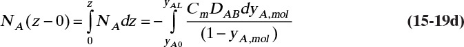
For absorbers and strippers (see Section 16.4) the film model is often used. We again postulate a film of thickness Δ, in which mass transfer occurs by diffusion only. This is shown in Figure 15-6 for absorption with gas-phase mass transfer controlling. In absorption carrier gas B often does not absorb; thus there is a stagnant layer of B, NB = 0. Then from Eq. (15-19c),
The solution obtained in Example 15-3, Eq. (15-20a), can be written for transfer between phases as
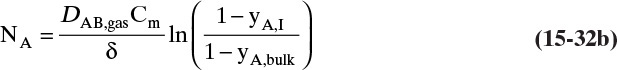
In this equation yA,I is the mole fraction of A at the interface (see Figure 15-6), and yA,bulk is the mole fraction of A in the bulk of the gas. Equation (15-32b) can also be written as

The log mean differences (1 – yA)lm and (yB)lm are defined as
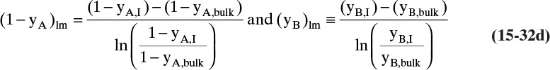
Note that as yA → 0 (very dilute systems), (1 – yA)lm → 1, and Eq. (15-32c) simplifies to (15-26a).
The reason for doing this rather convoluted algebra is that for concentrated systems with NB = 0, if we define the concentrated mass transfer coefficient as
then the flux becomes
which mimics the flux for dilute systems, Eq. (15-26b). This analysis can also be done based on partial pressure differences and a log-mean partial pressure difference (see Problem 15.C3). The concentrated system analysis is used in Section 16.4.
15.4.3 Binary Mass Transfer to Expanding or Contracting Objects
Shrinking or expanding bubbles, drops, or particles with rate of expansion or shrinkage controlled by mass transfer commonly occur in separations and reactions. The generic situation for any expanding or shrinking object in a fluid is shown in Figure 15-7. The linear driving-force model is used to simplify a rather complex problem. Analyses in this section and in Section 15.7.7 involve coupling unsteady mass balances with mass-transfer equations and then integrating the resulting differential equation. This section also provides opportunity to review and practice calculus.
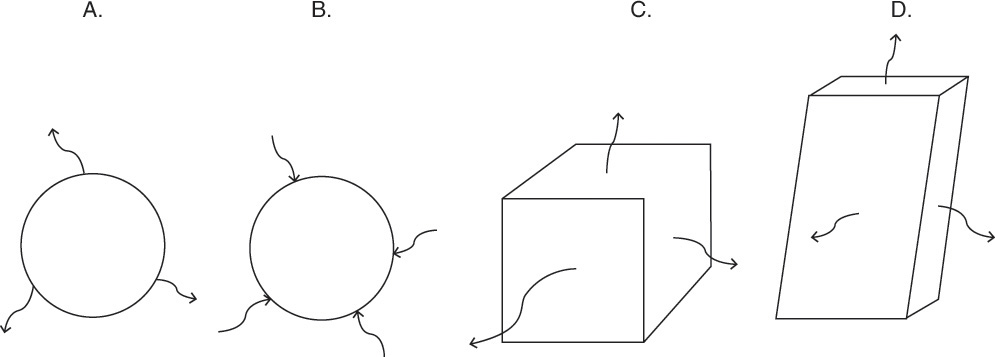
FIGURE 15-7. Mass transfer to or from submerged objects. A. Contracting sphere, B. Expanding sphere, C. Dissolving cube, D. Dissolving platelet
In this section we consider situations in which only mass transfer outside the object is important. This will be the case if the mass transfer rate inside the object is much greater than the rate outside the object or if the object is a pure compound (e.g., a bubble of oxygen). Chapter 16 explores interphase mass transfer where transfer rates on both sides of the interface are important.
The mass balance for any object with no reaction occurring is
With a single mass transfer process this is

where m is the mass of the object, kg, and ![]() is the flow rate of mass due to mass transfer, kg/s. For inlet flow of mass
is the flow rate of mass due to mass transfer, kg/s. For inlet flow of mass ![]() > 0, and for outlet flow of mass
> 0, and for outlet flow of mass ![]() < 0. The mass of the object can be determined from the volume and the density of the object, and the mass flow rate can be determined from the flux and the area for mass transfer:
< 0. The mass of the object can be determined from the volume and the density of the object, and the mass flow rate can be determined from the flux and the area for mass transfer:
The volume and areas for mass transfer depend on the geometry (see Table 15-5).
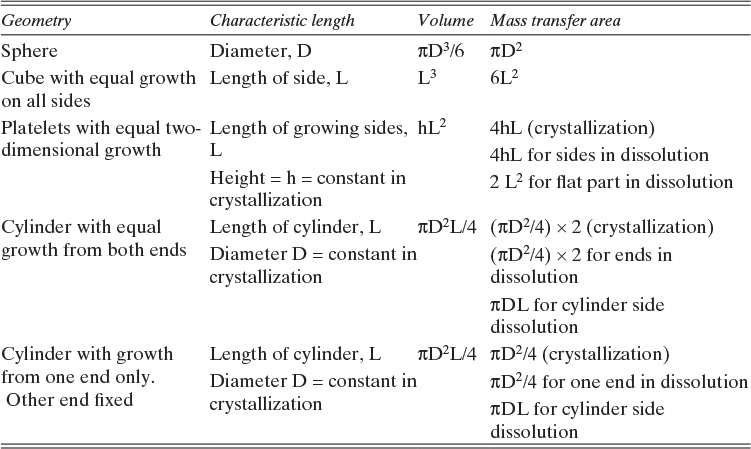
TABLE 15-5. Geometry of submerged objects. In crystallization growth may occur in only certain directions. In dissolution all directions dissolve
If the solute being transferred is dilute in the external fluid, then the mass flux is
where ρfluid, xA,bulk, and xA,I are mass density, bulk mass fraction of A, and interfacial mass fraction of A in the fluid external to the object. Determination of the value of interfacial mass or mole fractions depends on the physical situation. If xA > xA,I, the flux is into the object, and if xA < xA,I, the flux is out of the object.
Shrinking sphere. Small bubbles will be spherical, and the formulas for volume and mass transfer area are given in Table 15-5. The mass balance equation for a shrinking sphere is

If ρsphere is constant, after taking the derivative and switching the mole fraction difference to the positive quantity (xAI – xA,bulk), we obtain

Simplifying

Separating variables and taking the integral of both sides

Assuming that k, ρsphere, ρsolution, and (xA,i – xA,bulk) are constant and integrating
When we integrated, we assumed that (xA,i – xA,bulk) is not a function of time. In other words we assumed concentration profiles are established much more quickly than the time required for significant movement of the sphere boundary. This assumption is called the pseudo-steady-state assumption because the concentration profile was assumed to be at a steady state, although we know that it takes a finite amount of time to establish concentration profiles. Kmit and Shah (1996) analyzed when assuming pseudo-steady state is valid. The question becomes one of comparing time scale for shrinkage of the sphere to time scale for establishing the concentration profile. Concentration profiles develop rapidly if mass transfer coefficients are relatively high (gas systems or liquid systems with stirring or natural convection) and if the difference between xA,I and xA,bulk is small, which is automatically true in dilute systems but can also be valid in concentrated systems. Shrinkage (or growth) of the sphere will be slow if sphere density is much greater than the density of the continuous phase or if interfacial concentration is very low (low solubility). In this section and in Section 9.7.7 we analyze problems where pseudo-steady state is likely to be valid.
Dilute Gas Bubble. Up to this point the analysis has been general and is applicable for any shrinking sphere of pure A in a dilute fluid that satisfies the assumptions. Consider a bubble of pure, slightly soluble gas such as oxygen immersed in a nonvolatile liquid (e.g., cold water) that is not saturated with oxygen. Oxygen will transfer from the bubble to the liquid. If pressure and temperature are constant, the sphere density ρsphere will be constant. Gas and liquid are assumed to be in equilibrium at the interface. Equilibrium for sparingly soluble gases is given by Henry’s law, Eq. (12-1b), yA,mol,I = (HA/ptot)xA,mol,I written in terms of interfacial mole fractions.
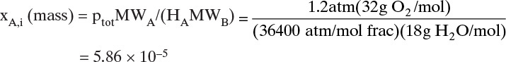
Since the problem has been presented in mass units, we need to convert Henry’s law to mass units. For sparingly soluble gas A in the liquid B the liquid will be almost pure B so that MWsolution = MWB, and ρsolution = ρB = constant. Then
and Henry’s law becomes
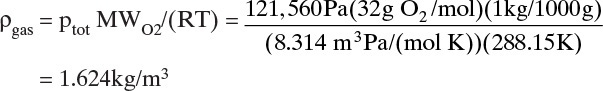
For a bubble of pure gas yA,mol,I = 1. The mass density of the sphere is the gas density, which for an ideal gas is
EXAMPLE 15-6. Shrinking diameter of oxygen bubble
A bubble of pure oxygen is in a tank of water that has been deoxygenated so that xO2,mol,bulk = xO2,mass,bulk = 0. If the initial diameter of the oxygen bubble is 1.5mm, what is the diameter after 750 s? Operation is at 1.2 atm and 15°C. The mass transfer coefficient is estimated as k = 1.2 × 10⁻⁵ m/s. MWoxygen = 32, MWwater = 18, R = 8.314 m3Pa/(mol K), ρwater = ρfluid = 1000 kg/m3. Henry’s law constants for oxygen for use in Eqs. (12-1b) and (15-37b) are in Table 15-6.

Source: Perry and Green (1984, p. 3–103)
TABLE 15-6. Henry’s law constants for oxygen in water (H is in atm/mol frac.)
The proper way to read Table 15-6 is that at 15°C, H = 3.64 × 10+4 atm/mol frac.
Solution
15°C = 288.15 K, 1.2 atm = 121,560 Pa. From Eq. (15-37b)
The density of the gas in the bubble is
At t = 1000 s Eq. (15-36) becomes
D = –2kρfluid(xA,I – xA,bulk)t/ρsphere + Dinitial
= –2(1.2 × 10⁻⁵)(1000)(5.86 × 10⁻⁵ – 0)(750)/(1.624) + 0.0015 = 0.000851 m
The pseudo-steady-state assumption is valid because of very low gas solubility and relatively high mass transfer coefficient. If ρfluid and (xA,I – xA,bulk) are constant, but the mass transfer coefficient k depends on mass fraction, Eq. (15-35d) will need to be integrated numerically.
Generalization: This and similar dilute problems can be solved by following these steps:
0. Determine if the pseudo-steady-state assumption is reasonable. If yes, proceed.
1. Write the mass balance equation, Accumulation = In – Out.
2. In and out terms due to mass transfer, ![]() , where NA = kΔCA.
, where NA = kΔCA.
3. Determine the interface concentration of A from equilibrium.
4. ![]() .
.
5. Determine area and volume from geometry (Table 15-5).
6. Determine k from appropriate correlation (Section 15-6).
7. Substitute terms into mass balance, expand derivatives, and simplify.
8. Integrate differential equation. If some terms are not constant, integration may have to be done numerically.
9. Find constant of integration from initial condition.
10. Substitute in values, and calculate desired answer.
Note: This problem has been oversimplified since there will be some mass transfer of water vapor into the bubble.
Evaporating Liquid Drop—Dilute System. Transferring our knowledge of what happens to gas bubbles in a dilute liquid to expanding or contracting liquid drops in a dilute gas is straightforward. The important word is dilute. For concentrated fluids we need to include convection in our calculation. Since small liquid drops tend to be spherical, equations for shrinking drops containing a pure liquid are identical to Eqs. (15-33a) to (15-33c) and similar to Eqs. (15-34) to (15-36). Of course we need to change notation in calculation of ![]() and use different equilibrium behavior at the interface. The pseudo-steady-state assumption will be valid because liquid density is much greater than gas density, ensuring that drops shrink or grow slowly. Since shrinking drops are more common, we consider that case.
and use different equilibrium behavior at the interface. The pseudo-steady-state assumption will be valid because liquid density is much greater than gas density, ensuring that drops shrink or grow slowly. Since shrinking drops are more common, we consider that case.
The interfacial mole fraction in the gas phase is given by Raoult’s law:
For a dilute system we can write Eq. (15-38a) in mass units as
For a pure liquid droplet xA,i,mol = 1, and
The mass balance for a shrinking sphere of liquid is

Except for the change in nomenclature, since mass transfer is in the gas phase, this equation is identical to Eq. (15-35a). We can make similar assumptions and take the same steps as were used from Eq. (15-35a) to Eq. (15-36) to obtain the result
For an ideal gas, the mass gas density is given by Eq. (15-37c) and yA,mass,i by Eq. (15-38c).
Evaporating Liquid Drop—Concentrated Systems. Since it is important to be comfortable working in both mass and mole units, we will switch to mole units. For an evaporating drop, the interfacial mole fraction of the gas yA,I is determined from Raoult’s law. For a pure liquid drop, xA,I (mole) = 1.0, and Raoult’s law becomes
If the rate of evaporation is modest, we can temporarily ignore the shrinkage of the drop (this is the pseudo-steady-state assumption). In this case solute A is being transferred through stagnant B and NB = 0. Then Eq. (15-32b) becomes
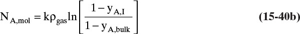
Density for an ideal gas is given by Eq. (15-37c), yA,i is from Eq. (15-40a), and yA,bulk is specified; thus we can calculate a numerical value for NA,mol. Then the mole balance is

Following the same sequence of steps used to derive Eq. (15-36), we obtain the following equation for the diameter of the spherical drop:
Since NA,mol is negative, the diameter of the drop decreases.
We can obtain some idea of how accurate setting NB,mol = 0 is by looking at the volume changes. Suppose the liquid (A) is water with a molar density of
ρliq,mol = (1,000,000g/m3)/(18 g/mol) = 55,556 mol/m3
The volume reduction of the liquid drop for a given time Δt is
Gas B has to diffuse to fill the volume vacated by the evaporating liquid, which requires
Setting Eqs. (15-41a) and (15-41b) equal and solving for ratio NB,mol/NA,mol, we obtain
At 101.3 kPa and 298 K the molar density of an ideal gas is ρgas,mol = 40.9 mol/m3. Thus
NB,mol/NA,mol = ρgas,mol/ρliq,mol = 40.9 × 10⁻⁷/0.00555 = 7.4 × 10⁻⁴
Although molar flux of gas B is not exactly zero, the percentage error is acceptably small.
Dissolving solid particle in dilute liquid. Solid particles of pure A will dissolve and shrink if concentration of A in the liquid is below its solubility limit. Dissolution often operates with quite high concentrations where convection occurs, and the pseudo-steady-state assumption is likely to be invalid. We will first consider a dilute system in which convection can be ignored and the pseudo-steady-state assumption is reasonable. Then a more concentrated system with a high mass transfer rate will be considered.
If the concentration in the liquid is above the solubility limit, then the particle will grow from crystallization or precipitation. Although mass transfer can be the rate-limiting step in crystallization, often other steps are rate limiting. Thus the analysis of growing solid particles is delayed until Chapter 17.
The basic equations for studying dissolution of solid particles in dilute systems are Eqs. (15-33a) to (15-33c) plus (15-34). Since crystals occur in a variety of shapes, Table 15-5 lists formulae for volume and area for mass transfer for the most common geometric shapes. Dissolving particles tend to decrease in size in all dimensions; however, mass transfer coefficients may be different for different faces of a crystal.
The mass balance for a cubic crystal dissolving at equal rates on all six faces is

Following the same steps used for Eqs. (15-35) to (15-36), we first assume that ρsolid is constant; take the derivative; simplify; assume that ρfluid, k, and (xA,bulk – xA,I) are constant; integrate; and determine the constant of integration from the initial length Linitial at t = 0.
This result is very similar to Eq. (15-36) for gas bubbles. The interfacial mass fraction in the liquid is assumed to be in equilibrium with the dissolving solid. Thus xA,I,mass = xA,solubility,mass. Solubility values require data that may be available in handbooks (e.g., Perry and Green, 1984) or may need to be obtained experimentally.
Crystals that grow in only one or two directions (cylinders and platelets in Table 15-5) usually dissolve in all three directions. For example, consider a platelet. The rate of change of the platelet mass is

The analysis becomes tractable if we assume that the dissolution from the flat sides occurs independently of dissolution from the four growth sides. Although this assumption is not valid for all crystals, it uncouples the two dimensions and allows for easy calculation of approximate solutions. On the two flat sides,
And on the four sides that grow during crystallization,
We can simplify these equations, assume kflat, kgrowth sides, ρliquid, and (xA,solubility,mass – xA,bulk,mass) are constant, and then integrate each mass balance independently. This derivation is left as an exercise (Problem 15.C9). Since for platelets h << L, if the mass transfer coefficients are the same order of magnitude, then the dissolution will be completed first in the h direction.
Dissolving solid particle in concentrated liquid. Kmit and Shah (1996) have flagged exactly this situation as one where pseudo-steady state may not be valid because solid and liquid densities are the same order of magnitude. In addition, interfacial concentration, given by xA,I,mol = xA,solubility,mol, may be quite high, and if only diffusion occurs, mass transfer is slow. Under these conditions dissolution of the solid is faster than the formation of the concentration profiles, and the pseudo-steady-state assumption is not valid. We will only consider cases in which the mass transfer coefficient k is quite high and the pseudo-steady-state approximation is reasonable. This will occur if the system is well stirred or has significant natural convection because of density differences.
For this system molar densities of solid and liquid are of the same order of magnitude. Thus assuming mass transfer occurs in a stagnant fluid is not appropriate. Instead, if we consider the volume argument in Eqs. (15-41a) to (15-41c) used to justify setting NB,mol = 0, we can reason by analogy that a reasonable choice for determining NB,mol is Eq. (15-41c) written for solid dissolution:
With Eq. (15-44a) as the relationship between NA and NB, substituting this expression into Eq. (15-17e) and substituting the result into Eq. (15-16e), we obtain an expression for NA that can be integrated. Substituting in k = DAB/Δ, the result is
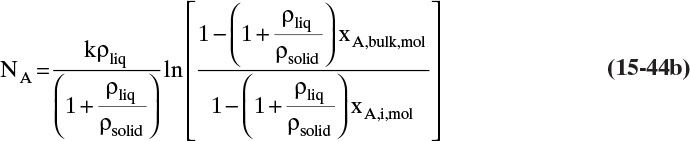
The derivation is left as a very useful exercise (problem 15.C4).
Equation (15-44b) gives a value for the molar flux. This value can be substituted into the mole balance [Eq. (15-33b) written in molar form]. The result is

where the volume term depends on the particle shape. Following the same sequence of steps used to derive Eq. (15-41), but for a solid particle, we obtain the following equation for the diameter of the spherical particle:
Since NA,mol is negative, the particle shrinks. Remember when using this equation that we have assumed that the pseudo-steady-state assumption is valid, which requires rapid mass transfer.
EXAMPLE 15-7. Dissolution of solid particle
A particle of pure NaCl is dissolving in an aqueous liquid solution at 18°C. The dissolution of the particle is controlled by mass transfer. The system is vigorously stirred, and the mass transfer coefficient k = 7.2 × 10⁻⁵ m/s (see Section 18.4.3 for stirred-tank mass transfer correlations). The aqueous solution is at NaCl mole fraction = 0.0932. Assume the system is ideal and the particle is spherical. If the initial particle diameter is Dinitial = 2.05 mm, find the time it takes to totally dissolve the particle. Data: Solubility of NaCl in water at 18°C = 9.99 mol%. MW NaCl = 58.45. Density pure solid NaCl = 2.163 g/cm3. Density of aqueous solution of NaCl = 1.20 g/cm3 (assume constant). MWwater = 18.016.
Solution
Preliminary calculations: Although mass liquid density is constant, because the mole fraction is changing, molar liquid density is not constant. We will use an average value ρliq,avg,mol. To find the average molar density, arbitrarily choose a basis of 10.0 moles of aqueous solution.
The average NaCl mole fraction is xNaCl,avg,mol = 0.5(0.0999 + 0.0932) = 0.09655. Then the average water mole fraction is xwater,avg,mol = 1 – xNaCl,avg,mol = 0.90345.
Mass NaCl = (10 moles solution)(0.09655)(58.45 g/mol) = 56.433 g.
Mass water = (10 moles solution)(0.90345)(18.016 g/mol) = 162.766 g.
Volume = weight/mass density = (56.433 + 162.766)/1.20 g/cm3 = 182.67 cm3.
Average molar density liquid = [10.0 mol/(182.67 cm3)] × [106 cm3/m3] = 54,740 mol/m3.
Molar density of solid = [(2.163g/cm3)(106cm3/m3)]/[58.45 g/mol] = 37,006 mol/m3.
From Eq. (15-44b),

The time to dissolve the particle can be found by setting D = 0 in Eq. (15-45b) and solving for t:
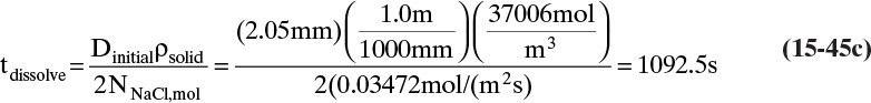
This is quite rapid because of the very high rate of mass transfer.
Comparison 1. Stagnant fluid calculation. If we do the calculation with the dilute Fickian equation (ignoring convection), we obtain
NA,mol = –k(xA,bulk – xA,i)ρliq,avg,mol = –(7.2 × 10⁻⁵ m/s)(–0.0067)(54,740 mol/m3) = 0.0264mol/(m2s)
and the dissolution time becomes tdissolve = 1436.3 s.
Comparison 2. Fickian with convection and NB = 0. If we assume NB = 0, then Eq. (15-32b) becomes
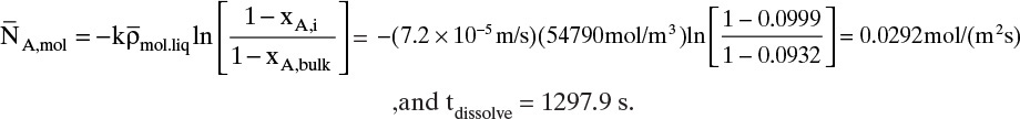
Note: For a single particle in a large amount of well-stirred solution, this solution is reasonable. In practical systems with a large number of particles dissolving, mole fraction of solution xA,bulk and solution density will both increase. Thus NA calculated from Eq. (15-44b) will decrease. Unless these changes are very slow (pseudo-steady state), mass balance Eq. (15-45a) will have to be integrated numerically. An additional mass balance based on tank size and number of particles that are dissolving is required to relate xA,bulk to operating time.
15.5 Correlations for Mass Transfer Coefficients
Intuitively, we expect that as temperature increases, molecules move faster (higher diffusivity) and k increases. In addition, if fluid flow is involved, we expect that a higher velocity or more mixing increases mass transfer rates. These intuitive ideas are generally qualitatively correct, but for engineering purposes we also need to be quantitative. Mass transfer correlations provide both qualitative and quantitative information needed for understanding and design.
In Section 15.5.2 we see that for simple physical situations such as steady-state mass transfer across a stagnant film, mass transfer coefficients can be determined analytically by solving the appropriate diffusion equations. Because actual processes often do not match assumptions required by theories, the resulting theoretical correlations often are not accurate. However, with a modest amount of data coefficients can be adjusted to provide significantly more accurate semi-empirical correlations. Many common and practical situations are complex and do not allow analytical solutions of the diffusion equation. For these cases empirical correlations for k or ka are often developed on the basis of dimensional analysis and experimental data. Dimensional analysis can predict probable forms for correlations, and experimental data is used to determine the exponents on the dimensionless groups and the value of the coefficient. A few mass transfer correlations are presented in this section, and a large number are summarized in Section 5B of Perry’s Handbook of Chemical Engineering (Wankat and Knaebel, 2008).
In simple geometries determination of area A in Eq. (15-1b), (15-1c), (15-2a), or (15-2b) is straightforward and is illustrated in this section. Membrane separators (Chapter 17) have areas A and areas per volume a that can be determined from straightforward geometric calculations. For more complex systems with interfacial mass transfer the value of interfacial area per volume a in Eqs. (15-3) and (15-4) and in the height of transfer unit (HTU) terms in Table 16-1 is more difficult to determine. Although a can be determined separately, it is more common to determine the product (ka). Correlations for (ka) in packed beds for distillation and absorption are discussed in Section 16.3. Correlations to calculate k and a separately in extraction mixers are discussed in Section 16.7. Correlations to estimate k in membrane separators are given in Section 18.4.3. Correlations for (ka) in adsorption, chromatography, and ion exchange are discussed in Section 19.6.3.
15.5.1 Dimensionless Groups
Correlations for mass transfer are often arranged into equations where all terms occur as dimensionless groups. One advantage is that any set of units can be used as long as the group remains dimensionless. A second advantage is that if the form of the correlation is not suggested by theory, dimensional analysis can be used to determine appropriate forms for the dimensionless groups.
Mass transfer correlations are often reported as the Sherwood number Sh, which is defined as

The Sherwood number is the ratio of the actual rate of mass transfer to the mass transfer due to diffusion alone. The appropriate length to use can be a film thickness, a diameter, or a plate length. The mass transfer coefficient can be either a local coefficient (e.g., at a given distance) or an average coefficient obtained by integrating the local coefficient over the entire distance. The dimensionless group defined in the first equation of Eq. (15-46a) is defined in terms of kc, which uses rate Eq. (15-24b). The second and third equations of Eq. (15-46a), which use kx or ky from rate Eqs. (15-24c) and (15-24d), need the total molar concentration Cm in the definition of the Sherwood number to make it dimensionless.
Mass transfer coefficients often depend on velocity, represented as a Reynolds number Re.

The Reynolds number is the ratio of inertial forces to viscous forces. In pipes the Reynolds number has the familiar form Re = Dvbρ/µ, but in other configurations, such as the flow of a liquid film down a flat plate, the definition can look superficially very different [e.g., see Eq. (15-56a)].
In correlations of gas or liquid data in separators, we often use the Peclet number Pe, which is the ratio of flow velocity to the diffusion velocity.
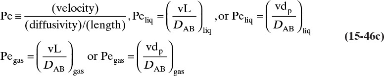
Forms of the Peclet number are shown with both column length L and particle diameter dp because both forms are used. It is obviously important to know whether L or dp is being employed in the definition of Pe. Sometimes a dimensionless group called the Stanton number St, which is the ratio of mass transfer velocity to flow velocity, is used.

The effect of the gas or liquid properties on mass transfer are taken into account in correlations by Schmidt number Sc, which can be considered the ratio of momentum diffusivity to mass diffusivity.

In Section 15.5.4 we consider the analogy between heat and mass transfer. The dimensionless group for heat transfer analogous to Sc is the Prandtl number Pr, which is the ratio of momentum diffusivity to thermal diffusivity.

The dimensionless group for heat transfer analogous to Sh is the Nusselt number Nu, which is the ratio of the actual rate of heat transfer to heat transfer due to thermal diffusion alone.
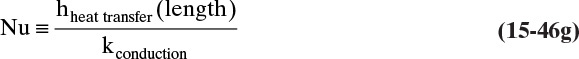
Since these dimensionless groups contain terms that depend on temperature and concentration, dimensionless groups depend on both temperature and concentration. In dilute systems concentration dependence is often negligible, and temperature-dependent solvent properties can be used.
15.5.2 Theoretically Derived Mass Transfer Correlations
If the physical situation closely matches assumptions made in development of theoretically derived mass transfer correlations, these correlations can be quite accurate. When physical situations are somewhat different than assumptions, correlations may still be useful by using a small amount of experimental data to tune coefficients. Practicing engineers seldom do derivations, but since they commonly use the results, it is important to know both assumptions and limits of validity of correlations. The best way to understand assumptions and limits is to closely follow derivations.
As a simple first example consider diffusion in a stagnant film (NB = 0) that was solved in Example 15-2 and a solution for constant total flux through the film that was given in modified form in Eq. (15-32c). Since total flux determined from diffusion and linear driving-force models, Eq. (15-32f), have to be equal, setting the equations equal for a film of known thickness δ we obtain
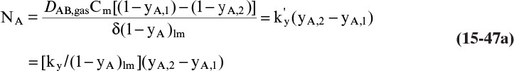
Solving for ky we obtain the simple result that
Substituting this result into Eq. (15-46a) the Sherwood number correlation for stagnant films is
Use of a linear driving-force model instead of a diffusion model [Eq. (15-32f) or for dilute systems Eq. (15-26b)] for this single-phase system would be unusual, but it could certainly be done. This development is for a gas film, but repeating it for a liquid film with liquid properties and liquid-phase, mass transfer coefficient kx is straightforward.
Generally, a linear driving force model is used when there is transfer between phases. The applications in Section 15.4.3 are examples. A classic problem that practically every mass transfer book includes is mass transfer from a gas to a falling laminar liquid film (Figure 15-8). This problem has practical significance, since falling films can occur in absorption, distillation, and stripping. In addition, the basic problem is mathematically interesting because it can be solved exactly with a series solution, and simple solutions are available for short residence times. Moreover, mass transfer becomes more complicated, requiring a semi-empirical correlation, as fluid velocity increases and ripples or waves form on the liquid surface. Finally, at even higher velocities, when the film becomes turbulent, empirical correlations are required. The theoretical model is considered in this section, and the semi-empirical and empirical models are considered in Section 15.6.3.
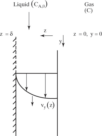
The diffusion equation for a falling liquid film (Figure 15-8) can be solved theoretically for absorption or stripping with the following rather restrictive set of assumptions:
1. Liquid flow is fully developed and laminar (will be relaxed in Section 15.6.3).
2. The film surface is flat (will be relaxed in Section 15.6.3).
3. Entering liquid has a constant, uniform concentration CA,init.
4. Gas-phase mass transfer rate is much greater than liquid-phase mass transfer rate. Thus surface concentration (at z = 0) is constant at CA,surf (will be relaxed in Section 15.6.3).
5. Diffusion rate in the liquid in the horizontal z direction is small, and convection in the z direction can be neglected.
6. The rate of convection due to the liquid flow in the vertical (y) direction is much greater than diffusion, and diffusion in the y direction can be neglected.
7. Plate width w is large enough that side-end effects can be ignored; thus velocity and concentration do not depend on the horizontal direction.
8. Diffusion coefficient DAB is constant.
9. The system is very dilute (this assumption is not necessary but simplifies the solution).
Solution for fluid velocity in a falling film is well known (Geankoplis, 2003; Treybal, 1980).
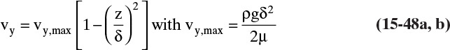
The average velocity and film thickness δ are
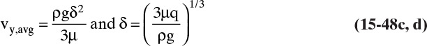
where q is the volumetric flow rate divided by the width of the plate [(m3/s)/m = m2/s]. The average residence time of fluid on the plate in seconds is
The steady-state mass balance states that (In – Out) of solute due to convection (in the y direction) equals (In – Out) due to diffusion (in the z direction). With constant diffusivity, this is

Taking the limits as Δy → 0 and Δx → 0 (assuming the limits exist), this equation becomes

Mathematically, this problem has a number of interesting characteristics. It has been solved for two different sets of boundary conditions. For relatively slow diffusion rates or short residence times (short length), solute from the liquid surface does not have time to penetrate to the wall. Boundary conditions are
These boundary conditions are the same as in Eq. (15-13) for unsteady diffusion. The answer is similar to Eq. (15-14b) and to Eq. (19-69) for adsorption. This result (modified from Geankoplis, 2003; and Cussler, 2009) is
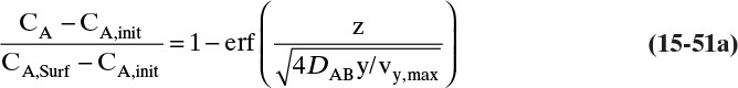
Error function is defined in Eq. (19-70), and values are tabulated in Table 19-7. Based on the following properties of the error function, Eq. (15-51a) satisfies boundary conditions in Eq. (15-50):

For a dilute system flux can be calculated from Fick’s law, Eq. (15-4a). From Eqs. (15-41), (15-51a), and (15-51b), at z = 0,

In general, for a system with NB,z = 0, the relationship between NA and JA is given by Eq. (15-32a). In dilute systems this simplifies to NA = JA, and Eq. (15-52a) becomes

For dilute systems linear driving force equations simplify to
Setting Eqs. (15-52b) and (15-52c) equal, we obtain for dilute systems at z = 0,
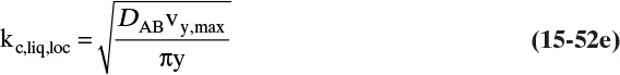
or in terms of the Sherwood number with length chosen as the film thickness δ, at z = 0 this is
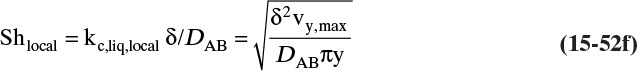
The local mass transfer coefficient depends on the value of y and is undefined at y = 0. Integrating Eq. (15-52b) over the range from y = 0 to y = L (the plate length), we obtain the total amount of solute transferred into the liquid at the surface of the liquid (z = 0):
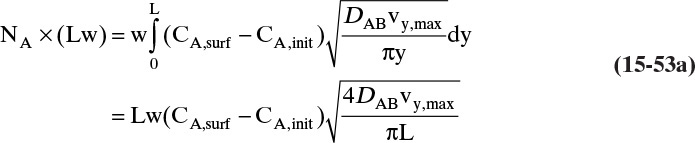
We can calculate the total transfer rate as NA,avg × (Lw). Setting this value equal to Eq. (15-53a) and solving for the average mass transfer coefficient and the average Sherwood number, we obtain

The alternative solution (Treybal, 1980; Sherwood et al., 1975) to Eq. (15-49b) does not assume that contact time is short and uses the boundary conditions

The last boundary condition at the solid wall implies there is no diffusion through the solid wall. Equation (15-49b) is more difficult to solve with this set of boundary conditions. The solution is an infinite series for the average concentration, leaving the film at y = L.

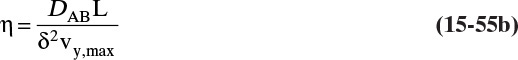
The total amount absorbed is the amount of solute exiting in the liquid minus the amount entering in the liquid:
This result can be related to NA,avg × (Lw), where the average flux for dilute systems is determined from Eq. (15-52d). Since CA,avg,L is given by an infinite series, this calculation is complicated. However, we can find limiting solutions for short contact times (large Reynolds number) and long contact times (small Reynolds number), where the Reynolds number for a falling liquid film is

For large values of Re, the result is Eq. (15-53b). Thus both analyses agree for short contact times. For long contact times (Re < 100 and large L), the average mass transfer coefficient and the Sherwood number for a system with no surface ripples are

Remembering that both δ and the Reynolds number increase as q increases, this result predicts that kc,liq,avg decreases as the Reynolds number increases. This is the opposite of what normally occurs, which is kc,liq,avg increases as the Reynolds number increases, as shown, for example, by Eq. (15-58). Thus in laminar flow, increasing velocity may not increase mass transfer coefficients or rates. Equation (15-53b) shows that at short contact times, the average mass transfer coefficient is proportional to ![]() , while Eq. (15-56b) shows that at long contact times kc,liq,avg is proportional to DAB.
, while Eq. (15-56b) shows that at long contact times kc,liq,avg is proportional to DAB.
If ripples are suppressed with a surfactant, these results are valid at least to Re = 250. Treybal (1980) reports that Eq. (15-56b) is valid to Re = 1200 if ripples are suppressed, while Sherwood et al. (1975) report that transition to turbulence occurs before a Reynolds number of 1200. This type of disagreement between sources is not unusual in mass transfer studies.
15.5.3 Semi-Empirical and Empirical Mass Transfer Coefficient Correlations
The results in Eqs. (15-53b) and (15-56b) assume that flow is laminar and the gas-liquid surface is flat. At Reynolds numbers less than 250, flow is laminar (Sherwood et al., 1975). However, even if fluid flow remains laminar, ripples can appear on the surface. Ripples cause local mixing, which increases the liquid-side mass transfer coefficient markedly, although mass transfer area increases only slightly. Addition of small quantities of surfactant (e.g., soap or proteins) eliminates ripples, and previously derived correlations for kc,liq,avg remain valid.
For long contact times (large L) Eq. (15-56b) will be valid if a surfactant is added or if Re < 20 (Wankat and Knaebel, 2008). For 20 < Re < 100 with no surfactant, the effect of ripples can be approximated by increasing kc,liq,avg by 40% to 100%. Then the coefficient in Eq. (15-56b) ranges from 4.77 to 6.82. With no other information, the average value can be used.
For short contact times (small L), Eq. (15-53b) can be used with ripples by multiplying kc,liq,avg by an average value of 1.7.

Obviously, a significant error is possible (±18%) for Eqs. (15-57a) and (15-57b) from just the multiplier for ripple formation. This type of error is not unusual for semi-empirical and empirical mass transfer correlations. These equations are semi-empirical because the basic form is from theoretical analysis, but the coefficient is from experimental data.
Sherwood et al. (1975) report that transition from laminar to turbulent occurs in the Reynolds number range from 250 to 500. Treybal (1980) reports the following correlation for a liquid film with constant surface concentration at a somewhat higher range of Reynolds numbers:

The Reynolds number Reliquid film for a liquid film is defined by Eq. (15-56a), and the Schmidt number that adjusts mass transfer coefficient for changes in liquid properties is defined in Eq. (15-46e). In dilute systems solvent properties can be used to calculate the Schmidt number.
If concentration of the liquid surface is not constant, there will be mass transfer and a mass transfer resistance on the gas side also. In separation processes, the gas-phase resistance often controls because gas-phase mass transfer coefficients are often significantly smaller than liquid-phase mass transfer coefficients. For turbulent flow of gas in a wetted wall tube, Gilliland reported the following correlation (see Sherwood et al., 1975; or Wankat and Knaebel, 2008).

Reevaluation of the data showed a better fit with (Wankat and Knaebel, 2008)

Both of these equations use a log mean gas mole fraction driving force, Eq. (15-32d). For mass transfer with a rippled surface, the gas-phase mass transfer correlation (Sherwood et al., 1975; Wankat and Knaebel, 2008) is

This equation agrees with Eq. (15-46a) when Reliq = 1000.
One additional common use of wetted-wall columns has been to study binary distillation. Johnstone and Pigford (1975) studied systems in which the gas mass transfer coefficient controlled. If partial pressure is used as the driving force, their correlation is

The modified Reynolds number is defined on the basis of the gas velocity relative to the surface of the liquid film. For countercurrent flow of gas and liquid, this is
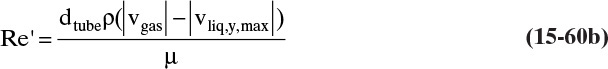
The term vliq,y,max is defined in Eq. (15-48b). Equation (15-60a) was used as the basis for mass transfer in each flow element of a structured packing to develop the first successful correlation for mass transfer in structured packings (Bravo et al., 1985).
A very large number of correlations are available in the sources referenced in this and later chapters. The purpose of showing these correlations is to show the types of forms that result, the need to know the range of validity, the need to know what difference or driving force is required, and the need to be very careful about the definition of terms.
EXAMPLE 15-8. Estimation of mass transfer coefficients
Water at 25°C is flowing down a 2.0 m long vertical plate at a volumetric flow rate per meter of plate width of q = 0.000045 m2/s (Figure 15-8). Entering (y = 0) water contains 0.9 g chlorine/kg water. The water is in contact with chlorine gas saturated with water vapor at 25°C (no water is evaporating). Chlorine is transferring into the water. At the water-gas surface (z = 0), water and chlorine are in equilibrium at the solubility limit of chlorine, CC12,surf. From Table 15-3, ![]() . At 25°C solubility of chlorine in water is 6.5 g/kg water, water density is 997 kg/m3, and viscosity is 0.9 × 10⁻³ kg/(m s).
. At 25°C solubility of chlorine in water is 6.5 g/kg water, water density is 997 kg/m3, and viscosity is 0.9 × 10⁻³ kg/(m s).
A. Determine film thickness δ, average vertical velocity in film, Reynolds number, and average mass transfer coefficient when surfactant is present. Per meter of plate width, at what average rate (kg/s) is chlorine transferred into water over the entire plate?
B. Repeat for q = 0.0018 m2/s.
Solution Part A
From Eqs. (15-48c) and (15-48d), we obtain
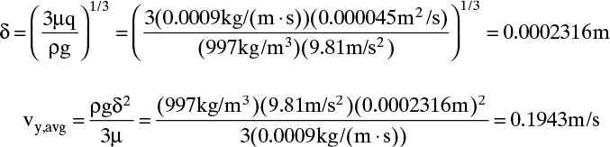
The average residence time of the liquid on the plate is
tres,avg = L/vy,avg = 2.0m/(0.1943m/s)= 10.29s
From Eq. (15-56a) the Reynolds number is
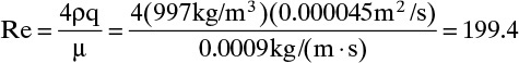
Since surfactant is added, ripples are suppressed, residence time is fairly long, and Re < 250; Eq. (15-56b) is applicable.

The chlorine concentrations in water in kg/m3 can be found from the mass ratios:

A similar calculation gives CC12,surface = 6.4805 kg/m3.
NA,avg = kc,liq,avg (CC12,surf – CC12,init)
Chlorine absorbed/m width = NA,avg × L
= (2.99 × 10⁻⁵m/s)(6.4805 – 0.8973kg/m3)(2.0m) = 0.0003337kg/(m· s)
Solution Part B
Repeating the calculations but with q = 0.0018 m2/s, we obtain
δ = 0.000792m, vy,avg = 2.2729m/s, tres,avg = 0.8799s, Re = 7976.
This Reynolds number indicates turbulent flow. Equation (15-58) is appropriate to determine the mass transfer coefficient. For this equation we need the value of the Schmidt number:

Then the Sherwood number is

And kc,liq,avg = 0.0007087 m/s. The Cl2 absorbed per m of width = 0.007913 kg/(m · s).
Comments
1. With turbulent flow the mass transfer coefficient is significantly higher, and more chlorine is absorbed despite the thicker layer of liquid and lower residence time.
2. Obviously, one needs physical property values. The viscosity, density, gas solubility, and the acceleration due to gravity g were all obtained from www.engineeringtoolbox.com.
2. Carrying dimensions through calculations is good practice and helps to catch errors.
15.5.4 Correlations Based on Analogies
In Section 15.2.1 we note that Fick derived his model for mass transfer partly by analogy to Fourier’s law of heat transfer and that one reason Fick’s model was rapidly accepted was this close analogy to Fourier’s law. Shortly after Fick’s developments, Osborne Reynolds stated that heat and mass transfer in a moving fluid should result from normal diffusion processes and eddies caused by fluid motion. Reynolds had not yet discovered the difference between laminar motion (only normal molecular diffusion operates) and turbulent motion (both molecular and eddy diffusion occur). We now know that Reynolds was correct only for turbulent flow.
Since I could not improve on it, I have closely followed Cussler’s (2009) development of Reynolds. Since eddies depend on fluid velocity, the easiest functional form is to assume eddy diffusion is linearly dependent on velocity. Then the mass transfer equation is
And in a similar fashion the equation for heat transfer is
For fluid flow, we introduce the friction factor f to find shear stress τ from the momentum ρv:

In highly turbulent flow, a terms (molecular diffusion) are much less than b terms (eddy diffusion) and can be neglected. Cussler notes Reynolds now took an amazing intuitive leap and concluded
This step says that transfer of mass, heat, and momentum by eddies is the same and requires
Quite logically, this is called Reynolds analogy. If we know either the heat-transfer coefficient h or friction factor f, we can estimate the mass transfer coefficient k. For gases Reynolds analogy is reasonably accurate, but for liquids it often fails.
Chilton and Colburn (1934) were able to empirically modify Reynolds analogy into a more robust analogy that works for gases and most liquids. Realizing that heat transfer would depend on fluid properties through the Prandtl number, Eq. (15-46f), and that mass transfer would depend on fluid properties through the Schmidt number, Eq. (15-46e), they included powers of Prandtl and Schmidt numbers in the first two terms of Eq. (15-62b). Fitting the resulting equation to experimental data showed that a power of 2/3 was appropriate and easy to use in calculations (very important in slide rule days). The result is
This equation is also written as
The definition of jD (the mass transfer term) is jD = (kc/v)(Sc)2/3, and the heat-transfer term jH is defined as jH = [hheat transfer/(ρCpv)](Pr)2/3. Even when the analogy is not being used, literature sources often give mass transfer correlations in terms of jD. If the definitions of the dimensionless groups from Eqs. (15-46a) and (15-46e) to (15-46g) are substituted in, the analogy can also be written as
Equations (15-63) apply to fully turbulent flow (although the equations also fit data for some laminar systems, such as flow past a flat plate) with a range of Schmidt number from 0.6 ≤ Sc ≤ 3000. Although not derived theoretically, there is some theoretical justification for these equations (Sherwood et al., 1975).
Because it is often easier to measure heat transfer than mass transfer, there are more heat-transfer correlations (usually in terms of Nusselt number) than mass transfer correlations (e.g., Incropera et al., 2011). Thus a major application of the Chilton-Colburn analogy is to estimate mass transfer coefficients or Sherwood numbers from existing heat-transfer correlations. In distillation mass transfer is more studied than heat transfer, and the Chilton-Colburn analogy is used to estimate heat-transfer coefficients in rate-based distillation models (Section 16.8).
Although very useful, the Chilton-Colburn analogy, as with all analogies, breaks down when the phenomena of heat transfer, mass transfer, and momentum transfer become different. For example, if radiation becomes important and is not separated from the heat-transfer term, then jD ≠ jH. If both skin friction and form drag (due to flow past blunt objects) occurs, then jD ≠ f/2 and jH ≠ f/2.
15.6 Difficulties with Fickian Diffusion Model
One difficulty with the Fickian diffusion model should be obvious from the discussion in Section 15.2.3. One has to select a somewhat arbitrary basis velocity or plane of reference to calculate convective and diffusive fluxes. Values and indeed meaning of convective and diffusive fluxes may change when the basis velocity is changed. Although irritating, this difficulty is not considered major because total fluxes of A and B, which are the purpose of the calculation, do not change.
There is an additional irritating problem. For liquid binary systems DAB usually depends on concentration, and although Eq. (15-22f) is often reasonably accurate, activity coefficient data may not be readily available. Even if activity coefficients are known, accurate prediction of infinite dilution diffusivities is difficult with current models (e.g., Sherwood et al., 1975; Wankat and Knaebel, 2008). Thus a significant amount of data may be required to accurately determine concentration dependence of binary diffusion coefficients in nonideal systems. Although this difficulty is significant, it can be overcome by dedicated laboratory analysis.
Finally, empirical extension of Fick’s law to systems with more than two components leads to logical inconsistencies and major calculation difficulties (Taylor and Krishna, 1993; Wesselingh and Krishna, 2000). For example, in ternary systems Fickian diffusion coefficients are not symmetrical, Di,j ≠ Dj,i; thus additional constants are required. In addition, values of Di,j depend on the value chosen for vref. Even worse, ternary systems can have a component diffuse into a more concentrated region or have no diffusion despite the presence of a concentration gradient (Taylor and Krishna, 1993). Accurately fitting this experimental data requires negative diffusivities.
The conclusions are that use of the Fickian model for binary diffusivities is reasonable, but the Fickian model is not suitable for systems with more than two components.
15.7 Maxwell-Stefan Model of Diffusion and Mass Transfer
In 1868, 12 years after Fick’s definitive publication of his theory, James Clerk Maxwell published a paper on a different approach to studying the diffusivity of gases. In 1871 Josef Stefan extended Maxwell’s theory and anticipated multicomponent effects (Cussler, 2009). Although the Maxwell-Stefan theory has had many strong adherents in the more than 140 years since its development, it always seems to be playing catch-up to the earlier Fickian theory. Three perceived difficulties have prevented wider acceptance of the Maxwell-Stefan theory. First, the Fickian model is well entrenched in textbooks and diffusivity data collections, and it works well for many binary systems. Second, the Maxwell-Stefan theory determines the relative fluxes, which gives one fewer flux Ni than is needed to completely solve the problem. Thus, the Maxwell-Stefan model requires finding another relationship to calculate all the fluxes and the total amount of mass transferred. However, this is really no different than choosing a reference velocity for Fick’s law, and, as is shown later, for most situations obtaining the additional flux equation is straightforward. Third, before digital computers made numerical solutions relatively simple (Taylor and Krishna, 1993), the differential form of the Maxwell-Stefan equations was considerably more difficult to solve than the Fickian equations. The development of difference forms of the Maxwell-Stefan equations (Wesslingh and Krishna, 1990, 2000) has helped to minimize this difficulty. Thus, in reality only the well-entrenched nature of the Fickian model currently prevents acceptance of the Maxwell-Stefan model.
The proponents of Maxwell-Stefan theory claim it is a better model than Fickian theory. What makes one model better than another model? First, it is nice to have a model tied to the basic physics or chemistry. A simple explanation based on the physics or chemistry should explain the basic behavior. This is illustrated for the Maxwell-Stefan model in Section 15.7.1. Second, the model should not conflict with well-accepted laws, such as the first or second law of thermodynamics. The Maxwell-Stefan model incorporates thermodynamics for the analysis of nonideal systems. Third, we want a model that can explain and/or predict data and that can be extrapolated. Except for ideal gas behavior diffusion models invariably have to use measured constants (diffusivity values). A good model minimizes the number of constants required and the variation of these “constants.” If the constants vary (say with concentration), the variation should be monotonic and preferably be close to linear. The constants for multicomponent systems should be predictable from binary pairs, and no impossible or improbable values (e.g., negative values) of the constants should be required to predict the data. Based on these criteria, the Maxwell-Stefan theory is a better theory than the Fickian model.
My advice is to learn to use both models. Learn the Fickian model in order to use the vast collections of solutions and data and to be able to communicate with other engineers. Learn the Maxwell-Stefan theory because its extra power allows relatively simple solutions to problems that are very difficult to solve with the Fickian model (e.g., nonideal binary systems and multicomponent systems).
15.7.1 Introductory Development of the Maxwell-Stefan Theory of Diffusion
The Maxwell-Stefan theory can be derived from continuum mechanics (Datta and Vilekar, 2010), irreversible thermodynamics (Bird et al., 2006), or kinetic theory of gases (Hirschfelder et al., 1964). Although the continuum mechanics approach is probably most powerful, for an introductory development a simplified kinetic theory is easier to follow. The presentations of Taylor and Krishna (1993) and Wesselingh and Krishna (2000) are paraphrased in a somewhat loose manner in this section.
Consider an ideal gas at constant pressure and temperature consisting of gases A and B. The entire system is moving at some average molar velocity vz,ref,mol. The coordinate system and control volume shown in Figure 15-9 are being translated at vz,ref,mol so that there is no net flow. As noted in Section 15.1 at normal pressures there are a huge number of molecules, and collisions between molecules occur repeatedly. If the two gases are moving through each other in the z direction, we can do a force balance for a control volume of thickness Δz shown in Figure 15-9. There are forces on molecule A due to partial pressure of A (pA × Area) at z, and at z + Δz,
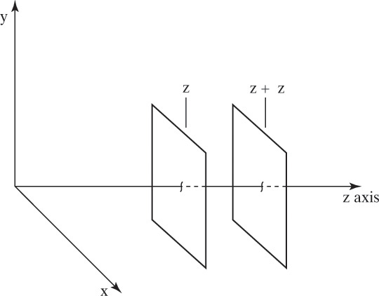
FIGURE 15-9. Coordinate system and control volume for Maxwell-Stefan derivation. The entire coordinate system is translating at vz,ref,mol
and there is a friction force caused by molecules of B flowing past molecules of A. Forces other than pressure and friction are assumed to be negligible but are easily included in the continuum mechanics treatment (Datta and Vilekar, 2010). We know that friction force is proportional to velocity differences of the two gases and amounts of each gas per volume of the segment. For an ideal gas, molar densities (amounts per volume) are
Then friction force is

Setting pressure force equal to friction force and taking limit as Δz → 0, we obtain

Noting pA = yAptot and pB = yBptot, and for constant total pressure and constant temperature incorporating term ptot/(RT)2 in a constant of proportionality fA,B this becomes

Term fA,B is a friction coefficient between molecules A and B, which are moving at average velocities vA and vB, respectively. Inverse of friction coefficient, ![]() , is the Maxwell-Stefan diffusivity. Since system pressure is constant, the left-hand side becomes –dyA/dz, and we obtain
, is the Maxwell-Stefan diffusivity. Since system pressure is constant, the left-hand side becomes –dyA/dz, and we obtain

The left-hand side of Eq. (15-65a) is the driving force for diffusion. The equation for component B is

If we substitute in the molar fluxes,
we obtain


It can be shown that these equations are equivalent to

Since the control volume in Figure 15-9 was set to move at the average molar velocity vz,ref,mol, there is no net flow, JB,z = –JA,z, which means
This equation requires
Thus binary ideal gas Maxwell-Stefan diffusivities are symmetric.
Equations (15-65) are different forms of the one-dimensional Maxwell-Stefan equations for a binary ideal gas at constant pressure and temperature. The equation can be written in three dimensions by replacing derivatives with gradients and velocities with vectors. For ideal binary systems, Section 15.7.5 shows that results obtained from the Maxwell-Stefan equations with ![]() is identical to results obtained with the Fickian diffusion equations.
is identical to results obtained with the Fickian diffusion equations.
15.7.2 Maxwell-Stefan Equations for Binary Nonideal Systems
For nonideal systems the generalized form of the driving forces in Eqs. (15-65) are based on the derivative of chemical potential µi (Datta and Vilekar, 2010; Krishna and Wesselingh, 1997; Taylor and Krishna, 1993; Wesselingh and Krishna, 2000). Since nonidealities are most common in liquids, we write the equations in terms of liquid mole fractions:
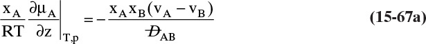
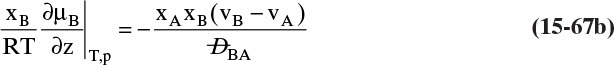
For ideal gases, the driving force on the left side of these equations reduces to (1/P)dpi/dz, which for constant pressure systems is equivalent to dyi/dz, and Eqs. (15-67) simplify to Eqs. (15-65a) and (15-65b). For nonideal systems chemical potential can be written in terms of activity coefficients γA and γB for liquids or the fugacity coefficients for gases. The results for component A for liquids are

or the equivalent form,

Since vA = NA,z/(xAρm) and vB = NB,z/(xBρm) where ρm is molar density, Eq. (15-68b) becomes

The corresponding equation for component B is

These forms are often useful in solving mass transfer problems. Obviously, detailed activity coefficient data or accurate correlations are required.
15.7.3 Determining Independent Fluxes Nj,z
Since the control volume in Figure 15-8 was set to move at average molar velocity vz,ref,mol, the sum of Jj,z is equal to zero for any system. Thus for a binary system only one Jj,z is independent. However, there are two independent fluxes, Nj,z. To use the Stefan-Maxwell formulation in practical problems, we need another relationship (called a bootstrap equation) that allows us to determine additional independent flux Nj,z. In other words, we need to tie moving Jj,z to stationary Nj,z. The additional equation depends on the situation. In general, Nj,z = Cjvj = Cmyjvj, and if one of the component transfer velocities vj is known, we can calculate the required unknown flux Nj,z.
Situation 1. Equimolar counter diffusion. In this case total flux Ntot,z = 0, vz,ref,mol = 0, and Nj,z = Jj,z. For a binary system NB,z = –NA,z and Eq. (15-69a) becomes

Situation 2. Distillation. If constant molar flow (CMO) is valid, then Ntot,z = 0, vz,ref,mol = 0, and Ni,z = Ji,z. For a binary system with CMO, Eq. (15-70a) is valid. If CMO is not valid, a reasonable approximation is ΣNi,z![]() i = 0, which for a binary is
i = 0, which for a binary is
Multicomponent distillation is treated in detail by Taylor and Krishna (1993).
Situation 3. Flow in a stagnant fluid. This situation can occur for condensation and evaporation when there is a noncondensing gas and for absorption and stripping. For binary systems the additional equation is NB,z = 0. This relationship leads to NA = JA/xB, which is the same result as for Fickian diffusion. For a ternary system, see Example 15-10.
Situation 4. Trace component is stagnant. This happens for dilute membrane permeation with concentration polarization. The result is NA,z = 0 and vz,ref,mol = 0.
Situation 5. Flux ratios are specified. If NA,z = (fracA)Ntot,z, then for a binary system, Eq. (15-69a) becomes
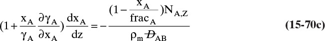
Situation 6. Chemical reaction. Reaction stoichiometry determines relationship. This topic is outside the scope of this text. See Taylor and Krishna (1993) or Wesselingh and Krishna (1990, 2000).
15.7.4 Maxwell-Stefan Difference Equation Formulations
Wesselingh and Krishna (1990, 2000) note that difference equations instead of differential equations are much easier to solve and, in most cases, result in answers that are of acceptable accuracy. For example, difference equations equivalent to Eqs. (15-68a) and (15-68b) are


The bars over terms mean they should be evaluated at the average conditions. If these equations are applied to mass transfer across a film, Δz = δ where δ is film thickness, we can define the average mass transfer coefficient in Maxwell-Stefan terms as ![]() . The resulting equations are
. The resulting equations are


Two additional useful forms can be obtained by substituting vA = NA/(xACm) and vB = NB/(xBCm) (where Cm is the total molar concentration) into Eqs. (15-71a) to (15-71d):
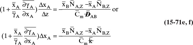
and

If the system is ideal, γA = 1, and the equations become

The forms in terms of the fluxes can be convenient in solving mass transfer problems.
The difference formula approximation can be made more accurate by doing several steps; however, since we need to know concentrations for the ends and center of each step, the usual method of dividing Δz into equal segments is awkward. The calculation is easier if segments are selected to give known mole fractions of A and each step size is unknown (see Problem 15.D18).
15.7.5 Relationship between Maxwell-Stefan and Fickian Diffusivities
Since most diffusivity data collected in the literature are based on Fickian diffusivity DAB and Fickian mass transfer coefficient ![]() , if we want to solve problems using the Maxwell-Stefan model, we must relate Maxwell-Stefan diffusivity
, if we want to solve problems using the Maxwell-Stefan model, we must relate Maxwell-Stefan diffusivity ![]() or mass transfer coefficient
or mass transfer coefficient ![]() to Fickian diffusivity DAB or mass transfer coefficient k. The relationship is relatively simple, although for nonideal systems it requires activity coefficient information to calculate
to Fickian diffusivity DAB or mass transfer coefficient k. The relationship is relatively simple, although for nonideal systems it requires activity coefficient information to calculate ![]() and
and ![]() .
.
For binary systems the relationships are
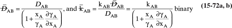
Since in the limit of infinite dilution γA = 1, Eqs. (15-72a) and (15-72b) require the infinite dilution limits of Maxwell-Stefan and Fickian diffusivities and mass transfer coefficients are equal.
Maxwell-Stefan diffusivities for approximately three-fourths of binary systems follow or approximately follow the empirical Vignes relationship (Wesselingh and Krishna, 1990):
This equation is Eq. (15-22f) converted to Maxwell-Stefan diffusivities. Comparison of this equation with the corresponding equation for Fickian diffusivity, Eq. (15-22f), shows that the equation for Maxwell-Stefan diffusivity is simpler and, for nonlinear systems where γ ≠ 1, Eq. (15-73a) will be closer to linear, which makes interpolation easier. Fewer data points are required to accurately fit an almost linear function than a more nonlinear one.
In ideal systems γA = 1 and
Ideality is most likely in low-pressure gas systems.
EXAMPLE 15-9. Maxwell-Stefan nonideal binary diffusion
A system of ethanol (E) and water (W) is undergoing equimolar counter diffusion across a thin liquid layer (δ = 0.000012 m) at 40°C and 1.0 atm. The boundary conditions are:
z = 0, xE (mole fraction) = 0.01, and at z = δ, xE = 0.3.
a. Estimate ![]() from infinite dilution values of diffusivity in Table 15-3 and Eq. (15-73a). Estimate molar density by assuming volumes are additive. Estimate flux of ethanol NE from the difference equation form of the Maxwell-Stefan equations. This calculation would be necessary if there were a minimal amount of data available.
from infinite dilution values of diffusivity in Table 15-3 and Eq. (15-73a). Estimate molar density by assuming volumes are additive. Estimate flux of ethanol NE from the difference equation form of the Maxwell-Stefan equations. This calculation would be necessary if there were a minimal amount of data available.
b. Calculate ![]() at xE = 0.155 from the activity coefficients and the values of the Fickian diffusivity in Table 15-4. Compare with the value estimated in part a.
at xE = 0.155 from the activity coefficients and the values of the Fickian diffusivity in Table 15-4. Compare with the value estimated in part a.
c. Estimate the flux NE using the diffusivity values in Table 15-4 and the difference equation form of the Maxwell-Stefan equations.
d. Compare the fluxes determined in parts a and b with the flux determined by numerical integration in Example 15-5.
Data: The activity coefficients for this system can be fitted to the van Laar equation:
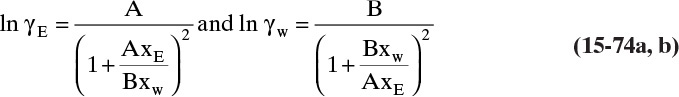
with A = 1.4599 and B = 0.9609 (Wesselingh and Krishna, 1990). At 40°C the molar densities of pure water is 55.08 kmol/m3 and of pure ethanol is 16.78 kmol/m3.
Solution Part A
For equimolar counter diffusion, NE,z = –NW,z, Eq. (15-71f) becomes
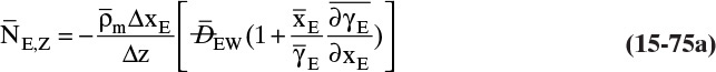
Estimation of Maxwell-Stefan diffusivity
xE,avg = (0.01 + 0.3)/2 = 0.155. Since the infinite dilution value of Maxwell-Stefan and Fickian diffusivities are identical, from Table 10-3 we obtain ![]() and
and ![]() . Equation (15-71a) becomes
. Equation (15-71a) becomes ![]() . At xE,avg = 0.155 the diffusivity is estimated as
. At xE,avg = 0.155 the diffusivity is estimated as ![]() .
.
Estimation of molar density
Choose a basis of 1.0 kmol of the mixture at xE,avg = 0.155. Then
Volume pure ethanol = 0.155 kmol/(16.78 kmol/m3) = 0.009237 m3.
Volume pure water = 0.845 kmol/(55.08 kmol/m3) = 0.01534 m3
Assume the volumes add. Then, total volume = 0.02458
Molar density ![]() .
.
Calculation of activity coefficient term
For the van Laar equation the derivative is (see Problem 15.C6)

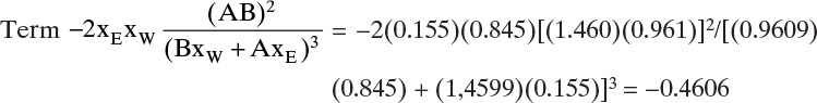
Estimation of flux
ΔxE = 0.30 – 0.01 = 0.29 and Δz = δ = 0.000012 m. Then Eq. (15-75) becomes
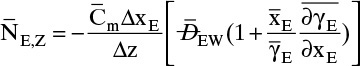
= –[40.69(0.29)/0.000012][1.6906 × 10–9(1 – 0.4606)] = –8.967 × 10⁻⁴ kmol/s
= –0.8967 mol/s
Solution Part B
The equation to calculate the Maxwell-Stefan diffusivity is
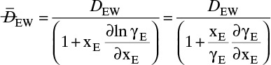
The Fickian diffusivity at xE = 0.155 can be obtained from Table 15-4 by linear interpolation. Using the values in Table 15-4 (DEW = 0.780 × 10⁻⁹ at xE = 0.144 and 0.680 × 10⁻⁹ at xE = 0.200) the linear interpolation equation is DEW (xE = 0.155) = 0.780 + (0.155 – 0.144)[(0.680 – 0.780)/(0.200 – 0.144)] = 0.7604, with all diffusivities multiplied by 10–9. For the van Laar equation the derivative was given in Eq. (15-74c). The calculation is
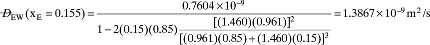
The estimated value was 21.9% high. The Vignes equation does not work well for the ethanol-water system.
Solution Part C
Substituting in the Maxwell-Stefan diffusivities from Eq. (15-72a), we find the term in brackets in Eq. (15-75a) is the Fickian diffusivity, and the result is

The value of ![]() can be estimated from Table 15-4 as 41.95 kmol/m3 by linear interpolation. The value of the Fickian diffusivity at xE,avg = 0.155 was determined in part b,
can be estimated from Table 15-4 as 41.95 kmol/m3 by linear interpolation. The value of the Fickian diffusivity at xE,avg = 0.155 was determined in part b, ![]() . Then
. Then
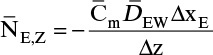
= –(41.95)(0.7604 × 10⁻⁹)(0.29)/(0.000012) = –7.709 × 10⁻⁴ kmol/s.
If the interval is divided into two parts (see problem 15.D18) NE = –9.408 × 10⁻⁴ kmol/s, with three parts NE = –10.642 × 10⁻⁴ kmol/s, and with four parts NE = –9.9465 × 10⁻⁴ kmol/s. Note that there is some oscillation in the answer.
Solution Part D
The calculation in Example 15-5 gave NE = –9.494 × 10⁻⁴ kmol/s with one area for Simpson’s rule and –9.732 × 10⁻⁴ kmol/s with two areas. The result from part c of this example using the finite difference approximation with the data for Cm and DEW was 20.8% low. The result from part a, NE = –8.967 × 10⁻⁴ kmol/s using an estimate of DEW based on Eq. (15-73a) was only 7.9% low. Usually we would expect the estimate using the extended data to be more accurate, but the highly nonlinear shape of the diffusivity data increased the error. However, if the interval for part c is divided into two parts, the error is 3.3%, with three parts the error is 9.4%, and with four parts the error is 2.2% (see Problem 15.D18).
Comments
1. The minus sign indicates that the direction of ethanol transfer is opposite to the direction of the z axis, which runs from z = 0 toward z = δ.
2. This is obviously an approximate solution, since we have estimated the derivative with one to four finite steps. When we divided the interval from z = 0 to z = δ into more parts, a more accurate answer was generated, although some oscillation in accuracy is observed.
15.7.6 Ideal Ternary Systems
The Maxwell-Stefan equations can be extended in a straightforward fashion to ternary and multicomponent systems. For an ideal ternary system, the basic equations are


Substituting in
we obtain


In difference notation Eqs. (15-77a) and (15-77b) become


The bars over the terms mean that average values should be used. In the film model for mass transfer the mass transfer coefficient is ![]() . Dividing the denominators of Eq. (15-65a) by Δz, we obtain
. Dividing the denominators of Eq. (15-65a) by Δz, we obtain
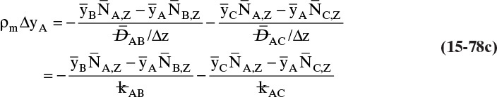

Unlike the Fickian diffusivities for ternary systems, the Maxwell-Stefan diffusivity is symmetric and is greater than or equal to zero for both ideal and nonideal systems. In ideal ternary systems, the Stefan-Maxwell diffusivities have the same values as the binary pairs, and as we already saw, the binary pairs have the same values as the Fickian binary pairs.
Unfortunately, the same condition does not hold for Fickian diffusivities. In an ideal ternary system, values for the Fickian diffusivities are not equal to values of the Fickian binary pairs.
For the limiting case of an ideal ternary that is quite dilute in one component (arbitrarily called component A), an effective Fickian diffusion coefficient for dilute component A can be calculated:

Substitution of this equation to replace DAB in Eq. (15-4a) allows calculation of the diffusion of dilute component A. Note that the effective diffusion coefficient depends on the concentrations of the other species. Although diffusion of the dilute component can be calculated accurately, diffusion of the concentrated components B and C probably will not be accurate (see Problem 15.H3b). Even for this special limiting case (ideal ternary with dilute component A), use of the Maxwell-Stefan equations is certainly preferable and not any more difficult than the Fickian method.
EXAMPLE 15-10. Maxwell-Stefan ideal ternary system
A ternary mixture of water (A), ammonia (B), and air (C) is being condensed in a heat exchanger. The bulk gas is 60.0 mol% water, 10.0 mol% ammonia, and 30.0 mol% air. The heat exchanger surface is at 42°C, and for simplicity in evaluating properties the entire operation is at 42°C and 1.0 atm. The condensed and dissolved water and ammonia in the liquid are assumed to have a high mass transfer coefficient so that gas-phase mass transfer controls. The diffusion is across a stagnant gas film (Figure 15-1) with δ = 0.01m thick. Determine fluxes (N values) of the three components.
Solution preliminaries
First, the air will not condense, and its solubility in the liquid is so low that it can be ignored. Thus Nair,z = NC,z = 0, and vc = 0.
At 42°C the Antoine equation (see Example 15-11) predicts a VP of water 61.354 mm Hg = 0.08073 atm and yw,surface = VPw/ptot = 0.08073.
This temperature is too hot for condensation of ammonia, but ammonia is very soluble in water. At 42°C and 1.0 atm the solubility of ammonia is 300 g NH3/1000 g water. Thus xNH3,saturation = 300/(1000 + 300) = 0.231. This value would occur if yNH3,surface = 1. We can use the saturation value of xNH3 to estimate the Henry’s law coefficient at 42°C. HNH3 = pNH3/xNH3 = (1.0)(1.0)/(0.231) = 4.329 atm. Then yw,surface = HNH3xNH3/ptot = 4.329xNH3/1.0, but neither yNH3,surface nor xNH3 are known. However, since all of the liquid on the heat exchanger comes from the transfer of water and ammonia to the liquid,
The problem is guess and check. We guess a value for xNH3, calculate yNH3,surface, complete the problem (conveniently formulated on a spreadsheet shown in this chapter’s appendix), and use Eq. (15-81) to determine xNH3,calculated. If the calculated value matches our guess, we cheer. Otherwise, continue the loop, but this is easily done automatically with either Goal Seek or Solver in Excel.
Solution of Maxwell-Stefan equations
Assume gas is ideal, and solve difference Eqs. (15-78a) and (15-78b). Parameters we need are ρm, DW-NH3, DW-Air, and DNH3-Air. Molar density of an ideal gas is ρm = ptot/(RT) = 1/(0.820575)(315) = 0.03869 kmol/m3. Fickian diffusivity DW-Air = 0.288 × 10⁻⁴ m2/s at 315 K and 1.0 atm (Table 15-1). At 273 K, DNH3-Air = 0.198 × 10⁻⁴ m2/s. This value was adjusted to 315 K by multiplying by (315/273)1.66 (see Example 15-4) with the result DNH3-Air = 0.251 × 10⁻⁴ m2/s. DW-NH3 was estimated as 0.212 × 10⁻⁴ m2/s from the Chapman-Enskog equation (see spreadsheet in chapter appendix). For an ideal system the Maxwell-Stefan binary-pair diffusivities are equal to the Fickian binary-pair diffusivities.
For water on the left-hand side of Eq. (15-78a),
Δyw / Δz = (yw,surface – yw,bulk) / (0.01m) = (0.1098 – 0.6) / .01 = –49.02
For NH3 in Eq. (15-78b),
ΔyNH3 / Δz = (yNH3,surface – yNH3,bulk) / (0.01m) = ((HNH3xNH3 / ptot) – 0.1) / .01
will depend on the current value used for xNH3.
On the right-hand sides of these equations, for water we have
and for ammonia,
which will change for each trial as the surface mole fraction varies.
At the surface air mole fraction is yair,surface = 1 – (yw,surface + yNH3,surface), which varies for each trial. Average ![]() also varies for each trial.
also varies for each trial.
For the final trial with xNH3 = 0.050958, yNH3,surface = 0.220597 and yair,surface = 0.698673. Average value for NH3 = 0.160299 and for air = 0.499336.
Δywater = 0.08073 – 0.6 = –0.51927 and ΔyNH3 = 0.220597 – 0.10 = 0.120597.
The two equations to be solved are


We now have two equations with the two unknowns ![]() and
and ![]() Solution of these two equations with the spreadsheet shown in this chapter’s appendix gives
Solution of these two equations with the spreadsheet shown in this chapter’s appendix gives ![]() and
and ![]() , which satisfy Eqs. (15-78a) and (15-78b). From Eq. (15-81) these values predict xNH3 = 0.050958, which matches the value used for the trial.
, which satisfy Eqs. (15-78a) and (15-78b). From Eq. (15-81) these values predict xNH3 = 0.050958, which matches the value used for the trial.
Comments
1. The actual solution of the difference form of the Maxwell-Stefan equations required less than a quarter of the total effort to solve this problem. Most of the effort arose because the need to know the surface concentration of ammonia in the vapor resulted in a trial-and-error problem.
2. A spreadsheet was used. Without it the guess-and-check solution would have been laborious.
3. Some care must be made in choosing trial values of xNH3. If this value is too large, NNH3 will be negative, which does not fit the problem analysis or Eq. (15-81).
4. Water behaves as expected in that its flux is in the downhill direction to a lower water mole fraction. Air has a concentration gradient (caused by changes in water and ammonia) even though there is no flux of air at steady state. Ammonia behaves counterintuitively (in a Fickian sense), since its flux direction is toward the higher mole fraction.
5. Since it is not a dilute ternary system, this problem is quite difficult to solve using the Fickian model.
6. Because the difference form of the Maxwell-Stefan equations was used, the answer is approximate. A more accurate answer can be obtained by a more accurate numerical solution of the differential equations (Taylor and Krishna, 1993).
7. Changing thickness of the gas layer is equivalent to changing the mass transfer coefficient ![]() and obviously affects the solution.
and obviously affects the solution.
15.7.7 Ternary Mass Transfer to Expanding or Contracting Objects
All of the binary systems analyzed with a Fickian linear driving force analysis in Section 15.4.3 can also be analyzed with the Maxwell-Stefan linear driving force analysis. The results are essentially identical (e.g., see Problem 15.D24).
For ternary mass transfer the Maxwell-Stefan procedure with difference equations is the easiest approach to develop approximate answers that can be quite accurate. In this section we will assume ideal gases. The total mole balance for an expanding/contracting object was Eq. (15-33b),

which is still valid, but rate of mass transfer can be due to any combination of the three components. In molar units the terms are

Equations (15-78c) and (15-78d) are used to determine flux. Terms in these equations can be estimated
Often the average mole fraction of component C will be found from
At this point we need a specific problem so that we can calculate interfacial mole fractions, densities, mass transfer coefficients, and the bootstrap relationship.
EXAMPLE 15-11. Ternary transfer from an evaporating drop
A drop of water containing CO2 is evaporating into air at 0.98 bar and 42°C. The initial drop size is 1.0 mm. Report the mole fractions of air at the interface and in the bulk, the fluxes of all three components, the diameter D of the drop after 10s, and the time when the drop disappears for the following:
A. 0.03 g CO2/1000 g water in the drop. ywater, bulk = 0, yCO2,bulk = 0.035.
B. 0.03 g CO2/1000 g water in the drop. ywater, bulk = 0.05, yCO2,bulk = 0.035.
Data: VP of water can be estimated from the Antoine equation:
log10 (VP) = 8.07131 – 1730.63/(T + 233.426)
where VP is in mm Hg and T in °C. Henry’s law coefficients for CO2 in water are listed in Table 12-1. Assume air is insoluble in water. Mass transfer coefficients: kw-air = 0.12 m/s, kCO2-air = 0.074 m/s, and kCO2-w = 0.076 m/s.
Solution
To write a general spreadsheet, let A = water, B = CO2, and C = air. The air is insoluble, so NC = 0. Flux equations are Eqs. (15-78c) and (15-78d) with NC = 0. Strategy: Solve for ![]() in Eq. (15-78c). In the spreadsheet guess a value of
in Eq. (15-78c). In the spreadsheet guess a value of ![]() , calculate
, calculate ![]() , and use Eq. (15-78d) to check if the guessed value of
, and use Eq. (15-78d) to check if the guessed value of ![]() was correct. If not, use Goal Seek to determine the value of
was correct. If not, use Goal Seek to determine the value of ![]() that satisfies Eq. (15-78d). The values were then substituted into the original equations to check that the solution was correct. We could also substitute the solution for
that satisfies Eq. (15-78d). The values were then substituted into the original equations to check that the solution was correct. We could also substitute the solution for ![]() into Eq. (15-78d) and then solve for
into Eq. (15-78d) and then solve for ![]() . This route was not chosen because it is relatively easy to make an algebraic mistake. Equation for
. This route was not chosen because it is relatively easy to make an algebraic mistake. Equation for ![]() with NC = 0 is
with NC = 0 is
This equation and Eq. (15-78d) (with NC = 0) were programmed into the spreadsheet (see Figures 15-A3 and 15-A4 in this chapter’s appendix). CO2: xCO2 = (0.03/1000) × (18/44) = 1.227 × 10⁻⁵. From Table 12-1 H = 2330 at 40°C and 2570 at 45°C. By linear interpolation at 42°C, H = 2426. yCO2,i = HxCO2/ptot = 2426(1.227 × 10⁻⁵)/[(0.98 bar/(1.0134 bar/atm)] = 0.03079. Water interfacial mole fraction yw,i = (VPw)xw/ptot. From Antoine equation VPw = 61.354 mm Hg = 0.081811 bar. xw = 1 – 1.227 × 10–5 = 0.999988, yw,i = 0.081811(0.999988)/0.98 = 0.083479.
Results:
A. Nw = 0.3834, NCO2 = 0.0006445 (+ flux is from drop to bulk), and Nair = 0 mol/(m2s), yair,i = 0.8857, yair,bulk = 0.965, at t = 10 s, D = 0.0008617 m, D = 0 at t = 72.325 s.
B. Nw = 0.1570, NCO2 = –0.006866 (+ flux is from drop to bulk), and Nair = 0 mol/(m2s), yair,i = 0.8857, yair,bulk = 0.915, at t = 10 s, D = 0.0009459 m, D = 0 at t = 184.98 s.
Problem 15.D25 lists three additional sets of data to simulate. Results for problem 15.D25 part c are shown in the spreadsheet in Figure 15.A4.
Observations: First, air has a gradient or driving force even though there is no flux of air. Second, CO2 flux can be in the direction opposite of Fickian predictions if ΔyCO2 is small and Δywater is large. Third, as expected, increasing the bulk mole fraction of water greatly decreased the water flux. The CO2 flux (run c) changed direction and was increased compared to run a.
15.7.8 Nonideal Ternary Systems
Unlike the Fickian model extension of the Maxwell-Stefan equations to nonideal ternary systems is straightforward. Equations (15-67a) and (15-67b) were the most general form of the Maxwell-Stefan equations for binary systems. For ternary systems these equations become


Expanding chemical potential µ in terms of activity coefficients, these equations become


If we note that vA = NA/(xAρm) and vB = NB/(xBρm) where ρm is molar density, we obtain


Converting these equations to difference equation form is left as an exercise (Problem 15.C10).
Multicomponent solutions are considered in detail by Krishna and Wesselingh (1997), Taylor and Krishna (1993), and Wesselingh and Krishna (1990, 2000). The Maxwell-Stefan matrix approach to multicomponent mass transfer is used in the Aspen Plus simulator to solve distillation problems. Use of computer simulators to obtain rate-based solutions of distillation problems is considered in Section 16.8 and in the appendix of Chapter 16.
15.8 Advantages and Disadvantages of Different Diffusion and Mass Transfer Models
In this section we briefly summarize advantages and disadvantages of each mass transfer model.
Molecular model. A molecular model has the advantage of explaining physically what is happening during diffusion, but the detailed theory is complex. The results [e.g., Eqs. (15-21a) to (15-21f)] are useful for predicting the diffusivity of gases. In its current state of development this model needs to be used in conjunction with another model for complicated mass transfer calculations. Use this model for physical understanding.
Fickian model. The Fickian model is a widely accepted model for diffusion, which means most engineers expect you to use it. It works well for ideal and close-to-ideal binary systems and can be used for nonideal binary systems if data are available. Most diffusivity data and correlations for mass transfer coefficients are based on the Fickian model. This model is very difficult to use for concentrated ternary systems and can require negative diffusion coefficients to predict data.
Linear driving force mass transfer model. This model is a widely accepted (by chemical engineers), empirical formulation that can be extended to very difficult mass transfer problems if empirical correlations for the mass transfer coefficient are available. The linear driving-force model based on Fickian diffusion is the model most commonly used for separation problems, but it can fail where the Fickian model fails. For ternary systems the linear driving-force model based on Maxwell-Stefan diffusion is more robust.
Maxwell-Stefan model. The Maxwell-Stefan model is generally agreed to be a better model than the Fickian model for nonideal binary and all ternary systems. However, it is not as widely understood by engineers, data collected in terms of Fickian diffusivities need to be converted to Maxwell-Stefan values, and the model can be more difficult to use. Use this model, coupled with a mass transfer model, when the Fickian model fails or requires an excessive amount of data.
Irreversible thermodynamics model. The irreversible thermodynamics model is useful in regions where phases are unstable and can split into two phases (deGroot and Mazur, 1984; Ghorayeb and Firoozabadi, 2000; Haase, 1990). However, this model is beyond the scope of this introductory treatment.
References
Bird, R. B., W. E. Stewart, and E. N. Lightfoot, Transport Phenomena, Revised 2nd ed., Wiley, New York, 2006.
Bravo, J. L., J. A. Rocha, and J. R. Fair, “Mass Transfer in Gauze Packings,” Hydrocarb. Proc., 64 (1), 91, (1985).
Chilton, Y. H., and Colburn, A. P., “Mass Transfer (absorption) Coefficients Prediction from Data on Heat Transfer and Fluid Friction,” Ind. Eng. Chem., 26, 1183 (1934).
Crank, J., The Mathematics of Diffusion, 2nd ed., Clarendon Press, Oxford, 1975.
Cussler, E. L., Diffusion. Mass Transfer in Fluid Systems, 3rd ed., Cambridge University Press, Cambridge, 2009.
Datta, R., and S. A. Vilekar, “The Continuum Mechanical Theory of Multicomponent Diffusion in Fluid Mixtures,” Chem. Engr. Sci., 65, 5976–5989, (2010).
deGroot, S. R., and P. Mazur, Non-Equilibrium Thermodynamics, Dover, New York, 1984.
Dean, J. A. (Ed.), Lange’s Handbook of Chemistry, 13th ed., McGraw-Hill, New York, 1985.
Demirel, Y., Nonequilibrium Thermodynamics, Transport and Rate Processes in Physical, Chemical and Biological Systems, 3rd ed., Elsevier, Amsterdam, 2013.
Geankoplis, C. J., Transport Processes and Separation Process Principles (Includes Unit Operations), 4th ed., Prentice Hall, Upper Saddle River, NJ, 2003.
Ghorayeb, K., and A. Firoozabadi, “Molecular, Pressure, and Thermal Diffusion in Nonideal Multicomponent Mixtures,” AIChE J, 46 (5), 892–900 (2000).
Haase, R. Thermodynamics of Irreversible Processes, Dover, New York, 1990.
Hines, A. L., and R. N. Maddox, Mass Transfer: Fundamentals and Applications, Prentice Hall, Upper Saddle River, NJ, 1985.
Hirschfelder, J., C. F. Curtiss, and R. Bird, Molecular Theory of Gases and Liquids, Revised Edition, Wiley, New York, 1964.
Hottel, H. C., J. J. Noble, A. F. Sarofim, and G. D. Silcox, “Heat Transfer,” in D. W. Green and R. H. Perry (Eds.), Perry’s Handbook of Chemical Engineering, 8th ed., McGraw-Hill, New York, 2008, Section 5a.
Incropera, F. P., D. P. DeWitt, T. L. Bergman, and A. S. Lavine, Fundamentals of Heat and Mass Transfer, 7th ed., Wiley, New York, 2011.
Johnstone, H. F., and R. L. Pigford, “Distillation in a Wetted Wall Column,” Trans. AIChE, 38, 25 (1942).
Kmit, J. M., and D. B. Shah, “Application of Pseudo-Steady-State Approximation in Solving Chemical Engineering Problems,” Chem. Engr. Educ., 30 (1), 14-18 (Winter 1996).
Kirwan, D. J., “Mass Transfer Principles,” in R. W. Rousseau (Ed.), Handbook of Separation Process Technology, Wiley-Interscience, New York, 1987, Chap. 2.
Krishna, R., and J. A. Wesselingh, “The Maxwell-Stefan Approach to Mass Transfer,” Chemical Engineering Science, 52, 861–911 (1997).
Marrero, T. R., and E. A. Mason, “Gaseous Diffusion Coefficients,” J. Phys. Chem. Ref. Data, 1, 3–118 (1972).
Poling, B. E., J. M. Prausnitz, and J. P. O’Connell, The Properties of Gases and Liquids, 5th ed., McGraw-Hill, New York, 2001.
Poling, B. E., G. H. Thomson, and D. G. Friend, “Physical and Chemical Data,” in D. W. Green and R. H. Perry (Eds.), Perry’s Handbook of Chemical Engineering, 8th ed., McGraw-Hill, New York, 2008, Section 2, Tables 2-324 and 2-325.
Sherwood, T. K., R. L. Pigford, and C. R. Wilke, Mass Transfer, McGraw-Hill, New York, 1975.
Taylor, R., and R. Krishna, Multicomponent Mass Transfer, Wiley-Interscience, New York, 1993.
Treybal, R. E., Mass Transfer Operations, 3rd ed., McGraw-Hill, New York, 1980.
Tyn, M. T., and W. F. Calus, “Temperature and Concentration Dependence of Mutual Diffusion Coefficients of Some Binary Liquid Systems,” J. Chem. Eng. Data, 20, 310–316 (1975).
Wankat, P.C., and K. S. Knaebel, “Mass Transfer,” in D. W. Green and R. H. Perry (Eds.), Perry’s Handbook of Chemical Engineering, 8th ed., McGraw-Hill, New York, 2008, Section 5B, pp. 5-1, 5-2, 5-43 to 5-83.
Wesselingh, J. A., and R. Krishna, Mass Transfer, Ellis Horwood, Chichester, England, 1990.
Wesselingh, J. A., and R. Krishna, Mass Transfer in Multicomponent Mixtures, Delft University Press, Delft, Netherlands, 2000.
Homework
A. Discussion Problems
A1. Suppose we have a volume of nitrogen plus a small amount of water vapor at 1.0 atm. The walls of the container are at 25°C, and there is a hot pipe at 105°C running through the volume. Explain the behavior predicted by Eq. (15-4a), the behavior predicted by Eq. (15-4b), and the reasons that Eq. (15-4b) more closely predicts reality.
A2. When is JA = NA, and when are they not equal?
A3. Explain why infinite dilution Fickian diffusivities for binary liquid systems are not equal,
A4. The constant in Eq. (15-22b) is 1.173 × 10⁻¹⁶, which agrees with Geankoplis (2003). However, Cussler (2009) and Wankat and Knaebel (2008) use a constant of 7.4 × 10⁻⁸. Both are correct. Explain.
A5. What is a controlling resistance? How do you determine which resistance, if either, is controlling?
A6. In Problem 15.H5 changing the pressure changes the diffusivities but does not change the Henry’s law constant of ammonia. However, changing the pressure does change the surface concentrations. Explain.
B. Generation of Alternatives
B1. In Example 15-1 operation is at a pseudo-steady state. Brainstorm alternative designs for this diffusion measurement.
B2. Although the additive approach traditionally used for coupling Fickian diffusion with convection appears logical and works for calculating total fluxes of A and B, this is not the only way one could tackle the problem. For binary systems this approach has the advantages of forcing DAB = DBA (see Problem 15.C1), and DAB is the same for any choice of vref (see Problem 15.C2). Instead of treating diffusion and convection terms as additive Eqs. (15-15a) and (15-15b), what other approaches could be used to analyze simultaneous convection and diffusion?
B3. Think of an experiment to measure diffusion coefficients that you could set up at home or in your apartment. Detail the equipment list. Estimate the amount of change you will observe. Will you be able to make accurate measurements? What could go wrong that will skew results?
B4. You have been invited to give a talk on mass transfer at the local high school. You want to show a live demonstration. Brainstorm at least five different demonstrations that you can develop with very simple apparatus—preferably made from standard cooking equipment.
B5. Develop roleplays to illustrate:
a. The difference between ordinary and Knudsen diffusion.
b. The difference between Fickian and Maxwell-Stefan diffusion.
C1. For binary diffusion with convection, use Eqs. (15-16a) to (15-16c) and equivalent equations for component B to show that DAB = DBA.
C2. For binary diffusion, show that DAB does not depend on the choice of vref.
C3. Derive the equation that is equivalent to Eqs. (15-32d) and (15-32e) in terms of a partial pressure driving force and a log mean partial pressure difference:
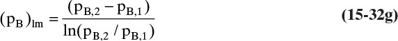
C4. Derive Eq. (15-44b).
C5. For binary Maxwell-Stefan diffusion through a stagnant layer of B, show that JA = NA/yB.
C6. Starting with Eqs. (15-74a) and (15-74b), derive Eq. (15-74c). Note: Because xW = 1 – xE, xW is not a constant.
C7. For binary distillation with CMO, vref,mol = 0. If CMO is valid, show that vref,mass ≠ 0 if MWA ≠ MWBA, and calculate the functional form for vref,mass that will make convection zero in this reference frame. Do this for diffusion in the vapor assuming an ideal gas.
C8. Derive Eq. (15-39b).
C9. For the dissolution of platelets in dilute solution show that
h = –2kflat ρliquid (xA,solubility,mass – xA,bulk,mass)/ρsolid + hinitial
L = –2kgrowth sides ρliquid (xA,solubility,mass – xA,bulk,mass)/ρsolid + Linitial
C10. Write the nonideal Maxwell-Stefan difference equations for a ternary system with the following Maxwell-Stefan mass transfer coefficient for each binary pair:
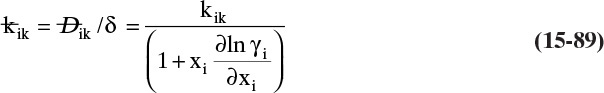
One approach is to pattern the steps after the development of the nonlinear binary Maxwell-Stefan equations [from Eqs. (15-68a) and (15-68b) to (15-71a) and (15-71b) to (15-71c) and (15-71d) to (15-71e) to (15-71h)]. The third component can be included following the pattern used for the ternary ideal Maxwell-Stefan Eqs. (15-76a) to (15-78d).
C11. Derive equation 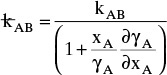 , assuming that
 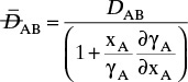 is valid.
D. Problems
D1. We have steady-state diffusion of 1-propanol across a liquid water film that is 0.10 mm thick. On one side of the film the 1-propanol concentration is 1.2 kg/m3. We desire a 1-propanol flux rate of 0.2 × 10⁻⁵kg/(m2s). The apparatus is at 25°C.
a.* What is the concentration at the other side of the film? Since the answer depends on the direction of transfer, there are two answers.
b. What are the equations for the concentration profiles?
Diffusivity value is given in Table 15-3.
D2. For the same system as in Problem 15.D1, the high concentration CA,0 = 1.2 kg/m3 and CA,L = 0.9701 kg/m3, which is same as in Problem 15.D1, but we want a flux rate = 0.35 × 10⁻⁵ kg/(m2s). Apparatus temperature can be adjusted. Estimate the Fickian infinite dilution diffusivity by adjusting the value from Table 15-3 for the temperature difference by assuming that Eo = 3000 cal/mol in Eq. (15-22c). What temperature is required?
D3. A column arrangement similar to Figure 15-2 is used for organic liquids. A large reservoir of water is under the column. The water is stirred and solute concentration in the water is constant. The organic liquid is immiscible in water and floats on the water surface at z = 0. Mole fractions x of the two layers in equilibrium are related by K = xsolute,organic/xsolute,water. At z = L = 20 cm (top of the column) mole fraction of solute in the organic liquid is zero. The entire apparatus is at 25°C and 1.0 bar. The column cross-sectional area is 0.55 cm2. Diffusion of solute, benzoic acid (C6H5COOH), in toluene (C6H5CH3) is studied. Assume toluene is totally immiscible in water. The mole fraction of benzoic acid in the water is kept constant at = 0.00212 mol%. Calculate benzoic acid flux in mol/(m2s).
Data: Diffusion coefficient of benzoic acid in toluene at 25°C = 1.5 × 10⁻⁹ m2/s.
MW toluene = 92.14 g/mol, MW water = 18 g/mol, MW benzoic acid = 122.12 g/mol. Density toluene = 865 kg/m3, density water = 1000 kg/m3.
K(25°C) = 123.1 = xbenzoic_acid_in_toluene/xbenzoic_acid_in_water.
D4. a. Estimate the Fickian diffusivity of a binary mixture of benzene and air at 298.2 K and 1.0 atm pressure using Chapman-Enskog theory and Table 15-2.
b. Compare your result with the experimental value in Table 15-3.
c. Estimate the Fickian diffusivity at 273 K and 0.5 atm.
d. Estimate Maxwell-Stefan diffusivity at 298.2 K and 1.0 atm.
D5. What is the Fickian diffusivity of chlorobenzene in liquid bromobenzene at 300 K when the mole fraction of chlorobenzene is 0.0332? Assume that the diffusivity follows an Arrhenius form and use the data in Table 15-3 to determine Eo. Also report the value of Eo in J/mol.
D6. Water at 60°C and 0.95 bar is evaporating into a 12.0-cm-long tube (also at 60°C) and diffusing through a stagnant layer of air. The device is illustrated in Figure 15-2.
a. Calculate the flux of water vapor if convection is included.
b. Calculate the value of the molar reference velocity.
c. If the tube is 1.5 cm in diameter, calculate the grams of water evaporated per hour.
d. Calculate flux of water vapor if convection is not included (a calculation that is expected to be incorrect for this example).
Data: At 60°C: Dwater – air = 3.05 × 10⁻⁵ m2 / s, VPwater = 149.5 mm Hg
D7. Assuming that the mixture is ideal, estimate infinite dilution Fickian diffusivities at 283.3 K for chlorobenzene in liquid bromobenzene and for bromobenzene in liquid chlorobenzene from data in Table 15-3.
D8. Use the Wilke-Chang theory to estimate infinite dilution Fickian diffusivity of methanol in liquid water at 293.16 K. Data are available at www.engineeringtoolbox.com and www.cheric.org/research/kdb.
b. Use a value of φB = 2.6.
D9. Determine the modified Sherwood number ![]() for gas-side-controlled mass transfer for distillation of ethanol-water in a wetted wall column. Column diameter is 10.0 cm. Measurements are at very low ethanol concentrations where flowing liquid can be assumed to be pure water. Total pressure is 1.0 bar. Liquid water at its boiling temperature is flowing down a vertical column at a volumetric flow rate per meter of circumference of q = 0.0000075 m2/s. Ethanol is diffusing through an upward-flowing vapor (almost pure water) at 1.0 bar and its boiling temperature. The upward vapor velocity is 0.81 m/s. Densities and viscosities of pure water liquid and pure water vapor are available in Perry’s Handbook of Chemical Engineering. Use parameters in Table 15-2 to estimate diffusivity of ethanol-water in the vapor.
for gas-side-controlled mass transfer for distillation of ethanol-water in a wetted wall column. Column diameter is 10.0 cm. Measurements are at very low ethanol concentrations where flowing liquid can be assumed to be pure water. Total pressure is 1.0 bar. Liquid water at its boiling temperature is flowing down a vertical column at a volumetric flow rate per meter of circumference of q = 0.0000075 m2/s. Ethanol is diffusing through an upward-flowing vapor (almost pure water) at 1.0 bar and its boiling temperature. The upward vapor velocity is 0.81 m/s. Densities and viscosities of pure water liquid and pure water vapor are available in Perry’s Handbook of Chemical Engineering. Use parameters in Table 15-2 to estimate diffusivity of ethanol-water in the vapor.
D10. A pipeline containing ammonia gas is vented to ambient air via a 20-m long, 3-mm diameter tube. What is the mass flow (g/day) of ammonia into the atmosphere? What is the mass flow of air into the pipeline (g/day)? Temperature and pressure everywhere are 25°C and 101,325 Pa, respectively. Assume pure ammonia at the pipeline and pure air at the air end of the tube. DAB = 2.8 × 10⁻⁵ m2/s (ammonia-air at 25°C). Assume ideal gas.
D11. We have steady-state diffusion of ammonia in air across a 0.033-mm-thick film. On one side of the film ammonia concentration is 0.000180 kmol/m3, and on the other side it is 0.000257 kmol/m3. What operating temperature is required to have an ammonia flux rate of 9.60 × 10⁻⁵ kmol/(m2s)? Pressure = 0.90 atm. Use the Chapman-Enskog theory to estimate diffusivity.
D12.* Water at 20°C is flowing down a 3.0-m long vertical plate at a volumetric flow rate per meter of plate width of q = 0.000005 m2/s. Entering (y = 0) water is pure. The water is in contact with carbon dioxide gas that is saturated with water vapor at 20°C (no water is evaporating). Carbon dioxide transfers into the water. At the water-gas surface (z = 0) water and carbon dioxide are in equilibrium at the solubility limit of carbon dioxide at CCO2,surf. Estimate Fickian infinite dilution diffusivity by adjusting the value from Table 15-3 for the temperature difference by assuming that Eo = 2000 cal/mol in Eq. (15-22c). At 20°C the solubility of carbon dioxide in water is 1.7 g/kg water.
a. Determine film thickness δ, average vertical velocity of film, and Reynolds number.
b. Is flow laminar? If no surfactant is added, do you expect ripples on the surface? If surfactant is added, do you expect ripples on the surface?
c. With no surfactant, determine average mass transfer coefficient and average Sherwood number.
d. Per meter of plate width, at what rate (kg/s) is carbon dioxide transferred into water over the length of the plate?
D13. Repeat all parts of Problem 15.D12 but with a water rate of q = 0.000015 m2/s.
D14. Repeat Problem 15.D12 but for q = 0.0015 m2/s.
a. Determine film thickness δ, average vertical velocity of film, and Reynolds number.
b. Determine average mass transfer coefficient and average Sherwood number.
c. Per meter of plate width, at what rate (kg/s) is carbon dioxide transferred into water over the length of the plate?
D15. We are measuring the diffusivity of water in air at 42°C. A tube is placed with one end in the water and the other end in a stream of dry air. The air column in the tube is 22-cm long, and we assume mole fraction of water is zero at the end in the air stream, ywater (z = 22) = 0. System pressure = 0.95 atm and is constant. At 42°C vapor pressure of water is 0.1098 atm, and diffusivity of water in air is DW-air = 2.88 × 10⁻⁵ m2/s. Assume ideal gases. Use the Maxwell-Stefan theory in difference equation form to determine flux of water at steady state.
D16. CO2 is being scrubbed out of a gas using water flowing through a packed bed. At the top of the bed CO2 is absorbed at a rate of 2.3 × 10⁻⁶ mol/cm2s. Inlet liquid is pure water, CO2 is present at a partial pressure of 10 atm, the Henry’s law constant is Hconc= 10,800 atm cm3/mol if Eq. (12-1a) is written as pB = CBHB,conc. The diffusion coefficient of CO2 in water is 1.9 × 10⁻⁵ cm2/s. Find the film thickness (δ). Assume that liquid phase resistance controls.
D17. Repeat Example 15-10 but with a mass transfer coefficient that is 10 times larger (use δ = 0.001 m). Report xNH3, yNH3,surface, Nwater, and NNH3.
D18.*
a. Repeat Example 15-9 part c, but divide the film into two parts (from 0 to Δz and from Δz to δ = 0.000012 m). Δz is unknown but is selected so that xE = 0.155 (the previous average point) at z = Δz. Now the average point for the first interval is xE = 0.0825 and for the second is xE = 0.2275. Since operation is at steady state, NE has to be the same in both intervals. Write Eq. (15-61e) for each interval (with thickness Δz for the first and δ – Δz for the second), and solve the resulting two equations for unknowns Δz and NE.
b. Divide the film into three parts (0 to Δz1, Δz1 to Δz2, and Δz2 to δ). Δz1 is unknown but is selected so that xE = 0.0825 at z = Δz1. Δz2 is also unknown but is selected so that xE = 0.2275 at z = Δz1 + Δz2. Since operation is at steady state, NE has to be the same in all three intervals. Write Eq. (15-61e) for each interval (with thickness Δz1 for the first, Δz2 for the second, and δ – Δz1 – Δz2 for the third), and solve the resulting three equations for unknowns Δz1, Δz2, and NE.
c. Divide the film into four parts, and determine NE.
*Answers are in Example 15-7, part c.
D19.* (Optional). Plot Figure 15-3 for the following unsteady diffusion problem. A thick layer of pure water (Cinitial = C∞= 0) at 25°C has a constant concentration of sucrose, C0 = 0.002 mol/L, placed on one surface at time t = 0. Assume the diffusivity (Table 15-3) is constant at the average concentration of 0.001 mol/L.
a.* Graph a plot C/C0 versus z (in cm) for t = 10,000 s. Selected values are in the answers at the back of the book.
b. If the measurement threshold of a zero concentration is 1.0 × 10⁻⁶ mol/L, what is the minimum thickness the layer must have to appear infinite at t = 100,000 s?
c. If the measurement threshold of a zero concentration is 1.0 × 10⁻⁶ mol/L, what is maximum exposure time the layer can have to appear infinite if layer thickness is 0.1 cm?
D20. Calculate the value of Maxwell-Stefan diffusivity for ethanol water at 40°C for ethanol mole fractions of 0.0, 0.2, 0.3, 0.4, 0.7, and 1.0. The Fickian diffusivities are available in Table 15-4. Which set of diffusivities are closer to linear?
D21. NaCl is crystallizing from an aqueous (water) liquid solution onto a crystal particle of pure NaCl at 18°C. Assume particle growth is controlled by mass transfer, and the particle is spherical. The aqueous solution is supersaturated at a mass fraction of NaCl = 0.30. If the initial particle diameter is D = 0.1 mm, find D after 3600 s.
Data: Solubility of NaCl in water at 18°C = 0.2647 mass fraction.
Density pure solid NaCl = 2.163 g/cm3. Molecular weight NaCl = 58.45.
Density of aqueous solution of NaCl = 1.20 g/cm3 (assume constant).
Density of pure water = 1.0 g/cm3. Molecular weight pure water = 18.
DNaCl-water at 18°C = 1.24 × 10⁻⁹ m2/s. Mass transfer coefficient k = 2.0 × 10⁻⁶ m/s.
D22. A 2-cm-diameter, 19-cm-long tube is placed touching a pool of liquid. The end away from the liquid pool (z = 0.19 m) is in an air stream (component C) so that it is pure air, yC (z = 0.19 m) = 1.0. The liquid is 80 mol% component A and 20 mol% component B. The ratio of these two components in the gas at z = 0 is the same as in the liquid, yA,i/yB,i = 4. The total vapor pressure of the liquid is 13,005 Pa. Thus 13,005/Ptotal = (yA,i + yB,i). Total pressure is 107,404 Pa, and temperature is 40°C. Assume ideal gas. At 40°C and 107,404 Pa, DAB = 2.45 × 10⁻⁵ m2/s, DBC = 2.69 × 10⁻⁵ m2/s, and DAC = 1.01 × 10⁻⁵ m2/s. MW B = 18, MW air = 28.9, MW A = 60.1. A partial solution is NA = 0.000228074 mol/(m2s). What are the molar fluxes, mol/(s m2), of B and C (air) at steady state?
D23. A crystal particle of pure NaCl is dissolving in an aqueous liquid (water) solution at 18°C. The dissolution of the particle is controlled by mass transfer. The aqueous solution is at a mass fraction of NaCl = 0.25.
Data: Solubility of NaCl in water at 18°C = 0.2647 mass fraction. MW NaCl = 58.45.
Density pure solid NaCl = 2.163 g/cm3.
Density of aqueous solution of NaCl = 1.20 g/cm3 (assume constant).
Density of pure water = 1.0 g/cm3. MW pure water = 18.
Diffusivity NaCl-water at 18°C = 1.24 × 10⁻⁹ m2/s. Mass transfer coefficient k = 1.8 × 10⁻⁶ m/s.
a. Assume the particle is spherical with an initial particle diameter D = 1.64 mm. Find the particle diameter after 7200 s.
b. Assume the particle is a cube with an initial particle length L = 1.64 mm. Find the particle length after 7200 s.
D24. Solve Example 15-7 using the difference equation form of the Maxwell-Stefan equations.
D25. Repeat Example 15-11 for the following conditions:
a. 0.03 g CO2/1000 g water in the drop. ywater, bulk = 0, yCO2,bulk = 0.05.
b. 0.00 g CO2/1000 g water in the drop. ywater, bulk = 0, yCO2,bulk = 0.0007.
c.* 0.03 g CO2/1000 g water in the drop. ywater, bulk = 0, yCO2,bulk = 0.0007.
* Answer is in a spreadsheet in Figure 15-A4.
D26.* Estimate ScV for a saturated vapor mixture that is 80 mol% ethanol and 20 mol% water at 1.0 atm.
E. More Complex Problems
E1. A short connecting pipe between two tanks is clogged with a plug of NaCl crystals. The plug formed as a cylinder of circular cross-sectional area with a constant diameter D = 2.0 cm and an initial length of 1.0 cm. The pipe is 2.0 cm in diameter and prevents the plug from increasing its diameter. However, the plug can grow or shrink from the two ends (it gets longer or shorter but has no change in diameter). The pipe is 10-cm long. Initially, the crystal is in the middle of the pipe from z = 4.5 to z = 5.5 cm. Tank 1 on the z = 0 side of the pipe contains pure water and is well mixed so that the bulk mass fraction of NaCl, xNaCl,1 = 0. Assume the solution density from z = 0 to the crystal plug is the density of water. Tank 2 on the z = 10 cm side contains a well-mixed, aqueous solution of NaCl with a mass fraction NaCl xNaCl,2 = 0.37. The rate of growth is controlled by mass transfer.
a. Find the length of the crystal plug after 104 seconds.
b. How far is the center of the plug from tank 1 after 104 seconds?
Data: Solubility of NaCl in water = 0.2647 mass fraction. MW NaCl = 58.45.
Density pure solid NaCl = 2.163 g/cm3.
Density of aqueous solution of NaCl with x = 0.37 is 1.22 g/cm3 (assume constant).
Density of pure water = 1.0 g/cm3. MW pure water = 18.
Mass transfer coefficient on side 1 (pure water) k1 = 5.5 × 10⁻⁶ m/s.
Mass transfer coefficient on side 2 (x2 = 0.37) k1 = 2.4 × 10⁻⁶ m/s.
The plug is cylindrical. Diameter is constant, and L varies.
H. Spreadsheet Problems
H1. Two identical, large glass bulbs are filled with gases and connected by a capillary tube that is δ = 0.0100 m long. Bulb 1 at z = 0 contains the following mole fractions: yair = 0.520, yH2 = 0.480, and yNH3 = 0.000. Bulb 2 at z = δ contains yair = 0.540, yH2 = 0.000, and yNH3 = 0.460. Since the bulbs are quite large, operation is at pseudo- (or quasi-) steady state. (In other words assume mole fractions at the boundaries are constant [e.g., yair = 0.520 at z = 0, and yair = 0.540 at z = δ so that Δyair = 0.02]) and total flux of air + hydrogen + ammonia is zero.] Pressure is uniform at 2.00 atm, and temperature is uniform at 273 K. Diffusivity values can be determined from Table 15-1. Assume ideal gases. Estimate fluxes of the three components using difference equation formulation of the Maxwell-Stefan method.
H2. Repeat Example 15-10 but for a bulk gas that is 40 mol% air, 15 mol% NH3, and 45 mol% water. Report xNH3, yNH3,surface, Nwater, and NNH3.
a. Repeat Problem 15.H1 (use the Maxwell-Stefan equations), but bulb 1 at z = 0 contains the following mole fractions: yair = 0.500, yH2 = 0.500, and yNH3 = 0.000. Bulb 2 at z = δ contains yair = 0.499, yH2 = 0.499, and yNH3 = 0.002.
b. Solve this problem using the effective Fickian diffusion coefficient for NH3, Eq. (15-67b), and usual Fickian equations for a very dilute system with no convection. Although there is not a simple approach for the two concentrated components, one is tempted to treat these as a binary with the Fickian binary diffusion coefficient for air and hydrogen. Try this method and then compare to solution of part a.
H4. Repeat Problem 15.H1, but bulb 1 at z = 0 contains the following mole fractions: yair = 0.520, yH2 = 0.480, and yNH3 = 0.000. Bulb 2 at z = δ contains yair = 0.520, yH2 = 0.000, and yNH3 = 0.480.
H5. Repeat Example 15-8 but for a pressure of 1.1 atm. Note that the diffusivities depend on pressure. Also answer problem 15.A6.
H6. A pipeline containing 99.0mol% ammonia and 1.0mol% hydrogen gas is vented to ambient air via a 15-m-long, 3.5-mm-diameter tube. Temperature and pressure everywhere are 0°C and 101,325 Pa, respectively. Assume 99.0mol% ammonia and 1.0 mol% hydrogen at the pipeline and pure air at the air end of the tube. Ideal gas, DAB = 1.98 × 10⁻⁵ m2/s (A = ammonia, B = air at 0°C), DCB = 6.11 × 10⁻⁵ m2/s (C = hydrogen, B = air at 0°C), DCA = 7.48 × 10⁻⁵ m2/s (A = ammonia, C = hydrogen at 0°C).
What are the molar fluxes, mol/(s m2), of ammonia, hydrogen, and air?
Chapter 15 Appendix. Spreadsheets Examples 15-10 and 15-11
The spreadsheet in Figures 15-A1 and 15-A2 solves Example 15-10. The spreadsheet is shown first with the formulas and then with numerical results. To estimate DW-NH3 from the Chapman-Enskog equation, the collision integral ΩD was estimated from the empirical fit in Eq. (15-21e). Goal Seek was used for the trial-and-error calculation of ammonia mole fraction.
FIGURE 15-A1. Spreadsheet for Example 15-10 with formulas
FIGURE 15-A2. Spreadsheet for Example 15-10 with results
The spreadsheets for Example 15-11 are shown in Figures 15-A3 (with formulas) and 15-A4 (with numerical results). In Figures 15-A3 and 15-A4 check in B15 is Eq. (15-78d) written in functional form (subtract right hand side so that equation = 0) × 1000 to decrease error in Goal Seek.
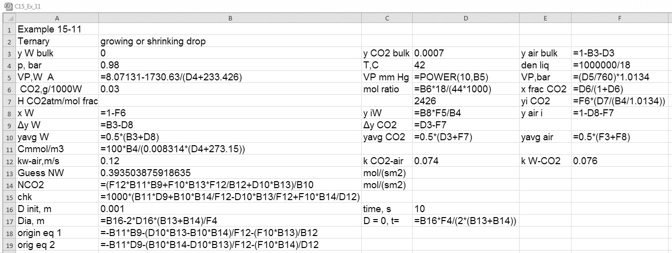
FIGURE 15-A3. Spreadsheet for Example 15-11 with formulas
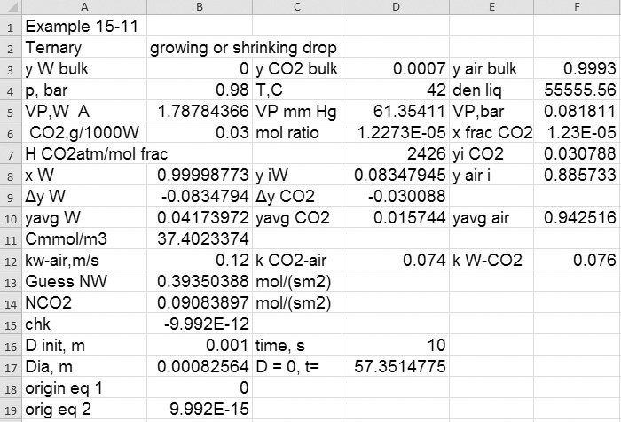
FIGURE 15-A4. Spreadsheet for Example 15-11 with results for problem 15.D25 part c