
Chapter 9. Batch Distillation
9.0 Summary—Objectives
In this chapter we explore batch distillation. After finishing this chapter, you should be able to satisfy the following objectives:
1. Explain the operation of simple and multistage batch distillation systems
2. Discuss the differences between batch and continuous operation
3. Derive and use the Rayleigh equation for simple binary batch distillation
4. Solve problems for constant-mole, batch distillation
5. Solve problems in batch steam distillation with a single volatile organic component
6. Use the McCabe-Thiele method to analyze multistage binary batch distillation for:
a. Batch distillation with a constant reflux ratio.
b. Batch distillation with a constant distillate composition.
c. Inverted batch distillation.
7. Solve problems for simple, multicomponent batch distillation.
8. Determine the operating time and energy requirements for a batch distillation
9.1 Introduction to Batch Distillation
Continuous distillation is a thermodynamically efficient method of producing large amounts of material of constant composition. When small amounts of material or varying product compositions are required, batch distillation has several advantages. In batch distillation a charge of feed is loaded into the reboiler, the steam is turned on, and after a short startup period, product can be withdrawn from the top of the column. When the distillation is finished, the heat is shut off, and the material left in the reboiler is removed. Then a new batch can be started. Usually the distillate is the desired product.
Batch distillation is a much older process than continuous distillation. Mesopotamian clay distillation pots have been dated to around 3500 B.C.E. (RT, 2007), and alchemists in Alexandria used simple batch retorts in the first century A.D. (Davies, 1980). Batch distillation was developed to concentrate alcohol by Arab alchemists around 700 A.D. (Vallee, 1998). It was adopted in Western Europe, and the first known book on the subject was Hieronymus Brunschwig’s Liber de arte distillandi, published in Latin in the early 1500s. This book remained a standard pharmaceutical and medical text for more than a century. The first distillation book written for a literate but not the scholarly community was Walter Ryff’s Das New gross Distillier Buch, published in German in 1545 (Stanwood, 2005). This book included a “listing of distilling apparatus, techniques, and the plants, animals, and minerals able to be distilled for human pharmaceutical use.” Kockmann (2014) thoroughly reviews the history of batch distillation. Advances in batch distillation have been associated with its use to distil alcohol, pharmaceuticals, coal oil, petroleum oil, and fine chemicals.
Batch distillation is versatile. A run may last from a few hours to several days. Batch distillation is used when the plant does not run continuously and batches must be completed in one or two shifts (8 to 16 h). It is often used when the same equipment distills several different products at different times. If distillation is required only occasionally, batch distillation is the usual choice.
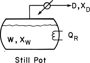
Equipment can be arranged in a variety of configurations (Sorensen, 2014). In simple batch distillation (Figure 9-1), the vapor is withdrawn continuously from the reboiler. The system differs from flash distillation in that there is no continuous feed input, and the liquid is drained only at the end of the batch. A similar alternative is constant-mole batch distillation in which solvent is fed continually to the still pot to keep the number of moles constant (see Section 9-4).
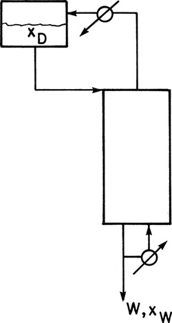
In a multistage batch distillation, a staged or packed column is placed above the reboiler as in Figure 9-2. Reflux is returned to the column. In the usual operation, distillate is withdrawn continually (Diwekar, 1995; Luyben, 1971; Mujtaba, 2004; Pratt, 1967; Robinson and Gilliland, 1950; Sorensen, 2014) until the column is shut down and drained. In an alternative method (Treybal, 1970), no distillate is withdrawn; instead, the composition of liquid in the accumulator changes. When the distillate in the accumulator is of the desired composition and in the desired amount, both the accumulator and the reboiler are drained. Luyben (1971) indicated that the usual method should be superior; however, the alternative method may be simpler to operate.
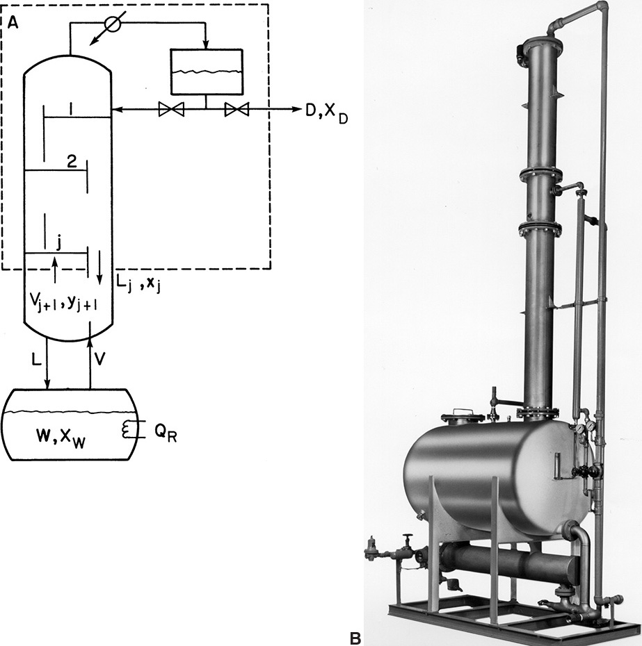
FIGURE 9-2. Multistage batch distillation; (A) schematic, (B) photograph of packaged batch distillation/solvent recovery system of approximately 400-gallon capacity. Courtesy of APV Equipment, Inc., Tonowanda, New York
Another alternative is called inverted batch distillation (Diwekar, 1995; Pratt, 1967; Robinson and Gilliland, 1950) because bottoms are withdrawn continuously while distillate is withdrawn only at the end of the distillation (see Figure 9-8 and Problems 9.C2 and 9.E3). In this case the charge is placed in the accumulator, and a reboiler with a small holdup is used. Inverted batch distillation is seldom used, but it is useful when quite pure bottoms product is required. Additional configurations include middle-vessel, multivessel, extractive, and hybrid (Sorensen, 2014).
9.2 Batch Distillation: Rayleigh Equation
The mass balances for batch distillation are somewhat different from those for continuous distillation. In batch distillation we are more interested in the total amounts of bottoms and distillate collected than in the rates. For a batch distillation, the overall mass balance around the entire system for the entire operation time is
The mass balance on any component, typically the light component is,
For a multicomponent feed Eq. (9-2) can be written for C-1 of the C components. The feed into the column is F kmoles of mole fraction xF of the more volatile component (MVC). At the end of the batch there are Wfinal kmoles of mole fraction xfin in the still pot. The symbol W is used since the material left in the reboiler is often a waste. Dtotal is the total kmoles of distillate of average concentration xD,avg. Equations (9-1) and (9-2) are applicable to simple batch and normal multistage batch distillation. Some minor changes in variable definitions are required for inverted batch distillation. If fractions are collected, Dtotal is split into a series of distillate fractions (see Section 9.2.2).
9.2.1 Mixed Distillate Product
A common way to operate simple batch distillation is to mix all the distillate and produce a single distillate product. Usually F, xF, and the desired value of either xfin or xD,avg for the light component are specified. An additional equation is required to solve for the three unknowns, Dtotal, Wfinal, and xfin (or xD,avg). This additional equation, called the Rayleigh equation (Rayleigh, 1902), is derived from a differential mass balance on the light component. Assume that the holdup in the column and in the accumulator is negligible. Then if a differential amount of material, –dW, of concentration xD is removed from the system, the differential component mass balance is
or
Expanding Eq. (9-4),
Then rearranging
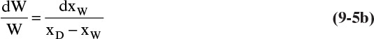
and integrating
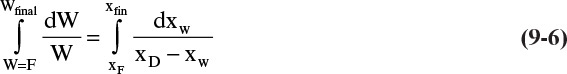
which is
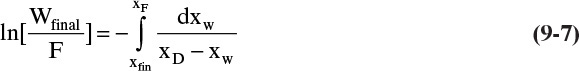
The minus sign comes from switching the limits of integration. Equation (9-7) is a form of the Rayleigh equation that is valid for both simple and multistage and for binary and multicomponent batch distillation. Of course, to use this equation we must relate xD to xW and do the appropriate integration. This is covered in sections 9.3 and 9.6. Time does not appear explicitly in the derivation of Eq. (9-7), but it is implicitly present since W, xW, and usually xD are all time dependent (see Section 9.8).
Once Wfinal has been determined D can be determined from the overall mass balance
and the average distillate concentration can be found from a mass balance on the MVC.

9.2.2 Distillate Product Fractions
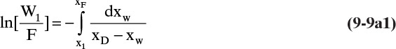
Another common operating method for batch distillation, particularly for multicomponent mixtures, is to collect different distillate fractions, 1, 2, 3, ..., with distillate amounts, D1, D2, D3, ..., collected when the still pot has W1, W2, W3, ... moles remaining in it with mole fractions x1, x2, x3, .... For the first period the Rayleigh equation is
The amount of distillate collected during this period is
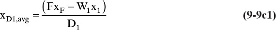
And the mole fraction of the component in this distillate fraction is
The initial amount in the still pot for the second period (essentially the feed for this period) is W1 with mole fraction x1. Then the Rayleigh equation, distillate amount, and distillate mole fraction become

The fractions continue until the last fraction n:

Equations (9-9) are valid for both simple binary batch and multistage binary batch distillation. If these equations are written for C-1 components, they are also valid for multicom-ponent systems.
If fractions with sharp cuts are desired, you can either add a large number of stages to the column or take a waste, or offcut, between the desired product fractions, as shown in Figure 9-3 (Sorensen, 2014). The offcuts are usually reprocessed in the next batch. Equations (9-9) are still valid, but some of the fractions are products, and some are offcuts. The taking of offcuts is explored in Problem 9.D26 for simple binary batch distillation.
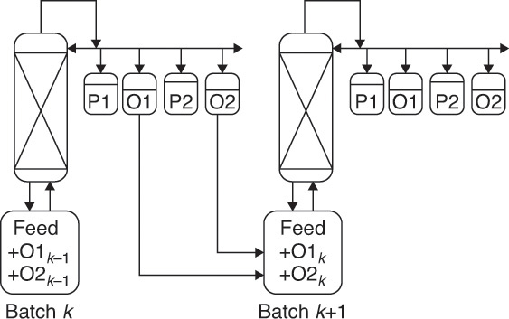
FIGURE 9-3. Batch distillation with distillate product cuts (P1 and P2) and offcuts (O1 and O2). From Sorensen, E., “Design and Operation of Bach Distillation,” in Gorak, A. and E. Sorensen (Eds.), Distillation. Fundamentals and Principles, Chapter 5, Elsevier, London, UK, 2014. Reprinted with permission of Elsevier. Copyright 2014.
9.3 Simple Binary Batch Distillation
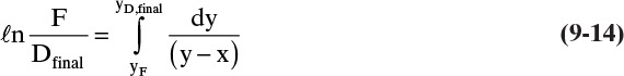
In the simple binary batch distillation system shown in Figure 9-1 the vapor product is in equilibrium with liquid in the still pot at any given time. Since we use a total condenser, y = xD. Substituting equilibrium into Eq. (9-7), we have
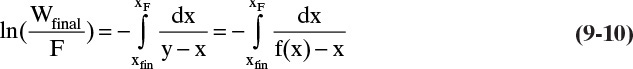
where y and x are in equilibrium with equilibrium expression y = f(x,p). For any given equilibrium expression, Eq. (9-10) can be integrated analytically, graphically, or numerically.
The general graphical or numerical integration procedure for Eq. (9-10) is:
1. Plot or fit the y-x equilibrium curve.
2. At a series of x values, find y – x.
3. Plot 1/(y – x) vs. x or fit it to an equation.
4. Graphically (Figure 9-4) or numerically integrate from xF to xfin.
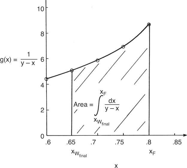
FIGURE 9-4. Graphical integration for simple batch distillation, Example 9-1
5. From Eq. (9-10), find the final charge of material Wfinal in the still pot:
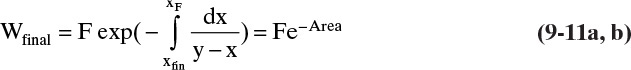
where the area is shown in Figure 9-4.
6. The amount of distillate, D, and the average distillate concentration, xD,avg, can be found from the mass balances Eqs. (9-8a) and (9-8b).
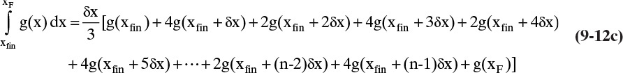
The Rayleigh equation can also be integrated numerically. One convenient method for doing this is to use Simpson’s rule (e.g., see Mickley et al., 1957, pp. 35–42; or Larsson et al., 2014, pp. 42–52). If the ordinate in Figure 9-4 is called g(x), then the simplest form of Simpson’s rule divides the interval into two equal parts with δx = (xF – xfin)/2.
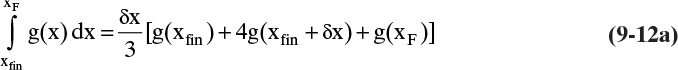
which is often written for batch distillation as

Terms are shown in Figure 9-4. Simpson’s rule is exact if g(x) is cubic or lower order. More accuracy can be obtained by dividing the interval into a larger, even number of parts of equal size. For example, if we use n equal subintervals, then δx = (xF – xfin)/n, and Simpson’s rule becomes
Note that n has to be an even integer. For smooth curves, such as in Figure 9-4, Simpson’s rule is quite accurate (see Example 9-1). For more complex shapes, Simpson’s rule may be more accurate if the integration is done in two or more separate pieces (see Example 9-2). Alternatively, half intervals can be used in regions where more accuracy is needed (Larsson et al., 2014). Simpson’s rule is also the MATLAB command quad (for quadrature) (Pratap, 2006). Other integration formulas that are more accurate can be used.
If the average distillate concentration is specified, a trial-and-error procedure is required. This involves guessing the final still pot concentration, xW,final, and calculating the area in Figure 9-4 either graphically or using Simpson’s rule. Then Eq. (9-11) gives Wfinal, and Eq. (9-8b) is used to check the value of xD,avg. For a graphical solution, the trial-and-error procedure can be conveniently carried out by starting with a guess for xfin that is too high. Then every time xfin is decreased, the additional area is added to the area already calculated.
If the relative volatility α is constant, the Rayleigh equation can be integrated analytically. In this case the equilibrium expression is Eq. (2-22b), which is repeated here:
Substituting this equation into Eq. (9-10) and integrating, we obtain

When it is applicable, Eq. (9-13) is obviously easier to apply than graphical or numerical integration. Analytical solutions for limiting cases (constant α in this case) are also useful for checking numerical solutions.
Warning: If α is not constant, Wfinal calculated from Eq. (9-13) can be very inaccurate.
EXAMPLE 9-1. Simple binary Rayleigh distillation
A simple batch still (one equilibrium stage) is separating a 50 mole feed charge to the still pot that is 80.0 mol% methanol and 20.0 mol% water. An average distillate concentration of 89.2 mol% methanol is required. Find the amount of distillate collected, the amount of material left in the still pot, and the concentration of the material in the still pot. Pressure is 1 atm.
Solution
A. Define. The apparatus is shown in Figure 9-1. The conditions are: p = 1 atm, F = 50, xF = 0.80, and xD,avg = 0.892. Find xfin, Dtot, and Wfinal.
B. Explore. Since the still pot acts as one equilibrium contact, the Rayleigh equation takes the form of Eqs. (9-10) and (9-11). To use these equations, either a plot of 1/(y – x)equil vs. x is required for graphical integration or Simpson’s rule can be used. Both are illustrated. Since xfin is unknown, a trial-and-error procedure is required for either integration routine.
C. Plan. First plot 1/(y – x) vs. x from the equilibrium data. The trial-and-error procedure is as follows:
Guess xfin.
Integrate to find 
Calculate Wfinal from the Rayleigh equation and xD,avg,calc from mass balance.
Check: Is xD,avg,calc = xD,avg? If not, continue trial and error.
D. Do it. From the equilibrium data in Table 2-7 the following table is generated:
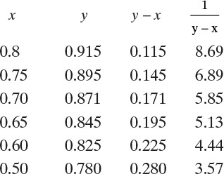
These data are plotted in Figure 9-4. For the numerical solution a large graph on millimeter graph paper was constructed.
First guess: xfin = 0.70.
From Figure 9-4,
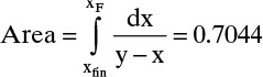
Then, Wfinal = F exp(–Area) = 50 e–0.7044 = 24.72
Dcalc = F – Wfinal = 25.28
The alternative integration procedure using Simpson’s rule gives
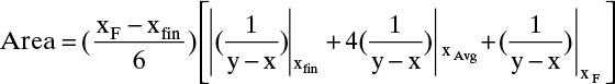
Where 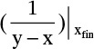 is the value of 1/(y – x) calculated at xfin, and xAvg = (xF + xfin)/2.
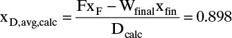
For Simpson’s rule, Wfinal = 24.79, Dcalc = 25.21, and xD,calc = 0.898. Simpson’s rule appears to be quite accurate in this case. Wfinal is off by 0.3%, and xD,calc is the same as the more exact calculation. These values appear to be close to the desired value, but we do not yet know the sensitivity of the calculation.
Second guess: xfin = 0.60. Calculations similar to the first trial give:
Area = 1.2084, Wfinal = 14.93, Dcalc = 35.07, xD,calc = 0.885 from Figure 9-4, and xD,calc = 0.884 from the Simpson’s rule calculation. These are also close, but they are low. For this problem the value of xD is insensitive to xfin.
Third guess: xfin = 0.65. Calculations give:
Area = 0.971, Wfinal = 18.94, Dcalc = 31.06, and xD,calc = 0.891 from Figure 9-4 and xD,calc = 0.890 from the Simpson’s rule calculation of the area, which are both close to the specified value of 0.892.
Thus, use xfin = 0.65 as the answer.
E. Check. The overall mass balance is Wfinal xfin + Dcalc xD,calc = 39.985 as compared to FxF = 40. Error is (40 – 39.985)/40 × 100, or 0.038%, which is acceptable.
F. Generalize. The integration can also be done numerically on a computer using Simpson’s rule or an alternative integration method. This is an advantage, since then the entire trial-and-error procedure can be programmed. Note that large differences in xW,final and hence in Wfinal cause rather small differences in xD,avg. Thus, for this problem, exact control of the batch system may not be critical. This problem illustrates a common difficulty of simple batch distillation—a pure distillate and a pure bottoms product cannot be obtained unless the relative volatility is very large. Note that although Eq. (9-13) is strictly not applicable since methanol-water equilibrium does not have a constant relative volatility, it could be used over the limited range of this batch distillation.
If xfin is very low, then 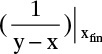 becomes very large, and Simpson’s rule is not very accurate. If the area is divided into two parts from xF to x ∼ 0.05 and from this point to xfin, Simpson’s rule will be accurate for the first part. Calculate Wfin,1 from Simpson’s rule. A reasonably accurate value of relative volatility can be estimated from αAB = (yA/xA)/(yB/xB) calculated from this point. Then Eq. (9-13) will give an accurate estimate of Wfin with F = Wfin,1 and xF set equal to the point used to divide the integral.
It is interesting to compare the simple binary batch distillation result to binary flash distillation of the same feed producing y = 0.892 mole fraction methanol. This flash distillation problem was solved previously as Problem 2.D1g. The results were x = 0.756 (compare to xfin = 0.65), V = 16.18 (compare to Dtotal = 31.06), and L = 33.82 (compare to Wfinal = 18.94). The simple batch distillation gives a greater separation with more distillate product because the bottoms product is an average of liquids in equilibrium with vapor in the entire range from y = 0.915 (in equilibrium with x = z = 0.8) to y = 0.845 (in equilibrium with x = xfin = 0.65), while for the flash distillation, the liquid is always in equilibrium with the final vapor y = 0.892. In general, a simple batch distillation will give more separation than flash distillation with the same operating conditions. However, because flash distillation is continuous, it is much easier to integrate into a continuous plant.
Extension of the solution method for simple binary batch distillation to collection of fractions is straightforward if the values of xW1, xW2, ... are specified. Equations (9-9) are converted to simple batch by replacing xD with y, which is in equilibrium with xW. In essence, a number of simple batch problems are solved sequentially (see Problem 9.D23).
Extension of the simple batch equations to multicomponent systems is also straightforward, although solution of the equations is significantly more difficult than solution of the binary equations. For simple multicomponent batch distillation Eq. (9-5b) becomes
The Rayleigh Eq. (9-10) can be written for each component. The equilibrium expression becomes a function of all the components, which couples all of the equations. Section 9.6 explores multicomponent simple distillation in detail.
A process that is closely related to simple batch distillation is differential condensation (Treybal, 1980). In this process vapor is slowly condensed, and the condensate liquid is rapidly withdrawn. A derivation similar to the derivation of the Raleigh equation for a binary system gives
where F is the moles of feed vapor of mole fraction yF, and Dfinal is the leftover vapor distillate of mole fraction yD,final. Differential condensation is rarely practiced.
9.4 Constant-Mole Batch Distillation
One relatively common application of batch distillation (or evaporation) is to switch solvents in a production process. For example, solvents may need to be exchanged prior to a crystallization or reaction step. Solvent switching can be done by charging the still pot with feed, concentrating the solution (if necessary) by boiling off most of the original solvent (some solvent needs to remain to maintain agitation, keep the solute in solution, and keep the heat transfer area covered), adding the new solvent, and doing a second batch distillation to remove the remainder of the original solvent. If desired the solution can be diluted by adding more of the desired solvent. Although this process mimics the procedure used by bench chemists, a considerable amount of the second solvent is evaporated in the second batch distillation. An alternative is to do the second batch distillation by constant-mole batch distillation in which the pure second solvent is added continuously during the second batch distillation at a rate that keeps the moles in the still-pot constant (Gentilcore, 2002). This section focuses on the constant-mole batch distillation step.
For a constant-mole batch distillation the general mole balance is
For the total mole balance this is In – Out = 0, since the moles in the still pot are constant. Thus, if dS moles of the second solvent are added, the overall mole balance for a constant-mole batch distillation is
where dV is the moles of vapor withdrawn.
If we do a component mole balance on the original solvent (solute is assumed to be nonvolatile and is ignored), we obtain the following for a constant-mole system,
where y and xw are the mole fraction of the first solvent in the vapor and liquid, respectively. Substituting in Eq. (9-15b), this becomes
Note that since the amount of liquid W is constant, there is no term equivalent to the last term in Eq. (9-4). Integration of Eq. (9-16b) and minor rearrangement gives us
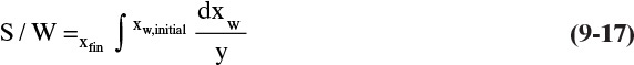
Since vapor and liquid are assumed to be in equilibrium, y is related to xw by the equilibrium relationship. Equation (9-17) can be integrated graphically or numerically in a procedure that is quite similar to that used for simple batch distillation. Problem 9.D17 leads you through these calculations for constant-mole batch distillation.
If constant relative volatility between the two solvents can be assumed, Eq. (2-22) can be substituted into Eq. (9-17), and the equation can be integrated analytically (Gentilcore, 2002):

Gentilcore presents a constant relative volatility sample calculation that illustrates the advantage of constant-mole batch distillation when it is used to exchange solvents. The method for obtaining accurate results for low values of xfin outlined in the last paragraph of Example 9-1 can be used for constant-mole batch distillation by replacing Eq. (9-13) with Eq. (9-18).
The amount of new solvent required can be reduced by putting a column above the still pot. Equation (9-17) remains valid except y is now the vapor leaving the top of the column (the same mole fraction as xdist if there is a total condenser), and y is not in equilibrium with the still-pot liquid. The procedures outlined in Section 9.6 for multistage systems can be used to determine the separation.
9.5 Batch Steam Distillation
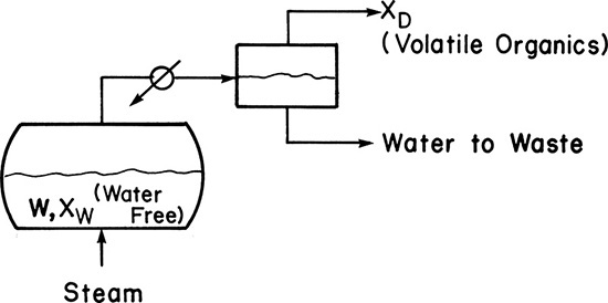
In batch steam distillation, steam is sparged directly into the still pot, as shown in Figure 9-5. This is normally done for systems that are immiscible with water. The reasons for adding steam directly to the still pot are that it keeps the temperature below the boiling point of water, it eliminates the need for heat transfer surface area, and it helps keep slurries and sludges well mixed so that they can be pumped. The major use is in treating wastes that contain valuable volatile organics. These waste streams are often slurries or sludges that foul heat exchanger surfaces and are difficult to process in an ordinary batch still. Glycerin, lube oils, fatty acids, and halogenated hydrocarbons are often steam distilled (Woodland, 1978). Section 8-3 is a prerequisite for this section.
Batch steam distillation is usually operated with liquid water present in the still. Then both the liquid water and the liquid organic phases exert their own partial pressure. Equilibrium is given by Eqs. (8-14) to (8-18) when there is one volatile organic and some nonvolatile organics present. As long as there is minimal entrainment, there is no advantage in the separation to having more than one stage, but steam use can be reduced. For low-molecular-weight organics, vaporization efficiencies, defined as the actual partial pressure divided by the partial pressure at equilibrium, p*,

are often in the range from 0.9 to 0.95 (Carey, 1950). This efficiency is close enough to equilibrium that equilibrium calculations are usually adequate.
The mass balances for Figure 9-5 are typically written on a water-free basis. These balances are identical in form to Eqs. (9-1) and (9-2) and can be solved for Wfinal if xfin is known.
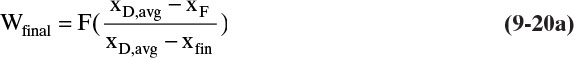
On a water-free basis F, Wfinal, and D are kmol organics in the feed, still pot, and distillate, respectively. The mole fractions x are (moles volatile organic)/(total moles organic). With a single volatile organic, xD,avg = 1.0 if entrainment is negligible. Then
and the amount of the organic distillate product is given by Eq. (9-8a), D = F – Wfinal. The Rayleigh equation can also be used and will give the same results.
At any moment the instantaneous moles of water dnw carried over in the vapor can be found from Eq. (8-18). This becomes

The total moles of water carried over in the vapor can be obtained by integrating this equation:
During the batch steam distillation, the mole fraction of the volatile organics in the still varies, and thus, the still temperature determined by Eq. (8-15) varies. Equation (9-21b) can be integrated numerically in steps. The total moles of water required is nw plus the moles of water condensed to heat the feed and still pot and to vaporize the volatile organics.
To integrate Eq. (9-21b) we must relate the moles of the volatile organic in the distillate, norg, to its mole fraction in the still pot, xpot = xvolatile. From a mass balance on the volatile organic very similar to that used to derive Eq. (9-20b), we obtain
This equation is valid at any time. As the mole fraction of the volatile organic in the still pot, xpot, decreases, the moles of volatile organic collected in the distillate, norg, increase.
For step-by-step numerical integration, Eq. (9-21b) can be written as
The total change in the mole fraction of volatile organic as xpot goes from xF to xw,final can be broken up into a number of intervals, Δxpot. In each interval norg, xpot,average, and Δnw are calculated. The amount of water carried over into the distillate with the volatile organic is given by Eq. (9-22c). The calculation becomes more accurate as more intervals are used in the range from xF to xw,final.
A short example for the simplified case in which the temperature in the still pot does not vary much and (VP)volatile is essentially constant will help to clarify the procedure. Suppose F = 1.0 kmol, xF = 0.35, Ptotal = 760 mm Hg, (VP)volatile = 50 mm Hg, and we want to calculate Δnw for a change in xpot from 0.25 to 0.20. Then from Eq. (9-22a) at xpot = 0.25,
norg = F(xF – xpot)/(1 – xpot) = 1.0(0.35 – 0.25)/(1 – 0.25) = 0.13333
At xpot = 0.20, norg = 0.18750. In the interval from xpot = 0.25 to xpot = 0.20, xpot,average = 0.225, and Δnorg = 0.18750 – 0.13333 = 0.05417. Then from Eq. (9-22b),
Δnw = 0.05417[760 – (50)(0.225)]/[(50)(0.225)] = 3.605 kmol water.
If the still pot temperature varies significantly, the temperature at each value of xpot,average needs to be determined from Eq. (8-15) so that the value of (VP)volatile can be calculated. This is easiest to do with a spreadsheet.
During most of the batch operation, the mole fraction of the volatile organic is considerably higher than it is at the end of the batch. In continuous steam distillation the mole fraction of the volatile organic is always at its lowest value. Thus, batch steam distillation requires less steam for a given separation than continuous steam distillation.
9.6 Multistage Binary Batch Distillation
The separation achieved in a single equilibrium stage is often not large enough to obtain both the desired distillate concentration and a low enough bottoms concentration. In this case a distillation column is placed above the reboiler, as shown in Figure 9-2. The calculation procedure is detailed here for a staged column, but packed columns can easily be designed using the procedures explained in Chapters 10 and 16.
For multistage systems xD and xW are no longer in equilibrium. Thus, the Rayleigh equation, Eq. (9-7), cannot be integrated until a relationship between xD and xW is found. This relationship can be obtained from stage-by-stage calculations. We assume that there is negligible holdup on each plate, in the condenser, and in the accumulator. Then at any specific time we can write mass and energy balances around stage j and the top of the column, as shown in Figure 9-2A. These balances simplify to
Input = Output
since accumulation was assumed to be negligible everywhere except the reboiler. Thus, at any given time t
In these equations V, L, and D are molal flow rates. These balances are essentially the same equations we obtained for the rectifying section of a continuous column except that Eqs. (9-23) are time dependent. If we can assume constant molal overflow (CMO), the vapor and liquid flow rates will be the same on every stage, and the energy balance is not needed. Combining Eqs. (9-23a) and (9-23b) and solving for yj+1, we obtain the operating equation for CMO:
At any specific time Eq. (9-24) represents a straight line on a y-x diagram. The slope will be L/V, and the intercept with the y = x line will be xD. Since either xD or L/V will have to vary during the batch distillation, the operating line will change continuously.
9.6.1 Constant Reflux Ratio
The most common operating method is to use a constant reflux ratio and allow xD to vary. This procedure corresponds to a simple batch operation in which xD also varies. The relationship between xD and xW can now be found from a stage-by-stage calculation using a McCabe-Thiele analysis. Operating Eq. (9-24) is plotted on a McCabe-Thiele diagram for a series of xD values. Then we step off the specified number of equilibrium contacts on each operating line starting at xD to find the xW value corresponding to that xD. This procedure is shown in Figure 9-6 and Example 9-2.
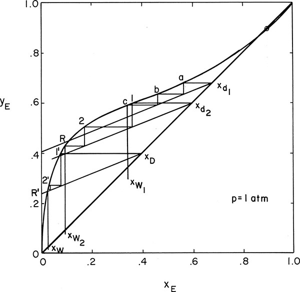
FIGURE 9-6. McCabe-Thiele diagram for multistage batch distillation with constant L/D, Example 9-2
The McCabe-Thiele analysis gives xW values for a series of xD values. We can now calculate 1/(xD – xW). The integral in Eq. (9-7) can be determined by either numerical integration, such as Simpson’s rule given in Eqs. (9-12a) to (9-12c), or by graphical integration. Once xW values have been found for several xD values, the same procedure used for simple batch distillation can be used. Thus, Wfinal is found from Eq. (9-7), xDavg from Eq. (9-8b), and Dtotal from Eq. (9-8a). If xDavg is specified, a trial-and-error procedure will again be required.
EXAMPLE 9-2. Multistage batch distillation
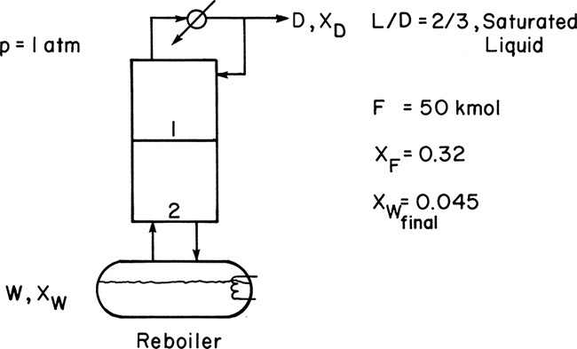
We wish to batch distil 50.0 kmol of a 32.0 mol% ethanol and 68.0 mol% water feed. The system has a still pot plus two equilibrium stages and a total condenser. Reflux is returned as a saturated liquid, and we use L/D = 2/3. We desire a final still-pot composition of 4.5 mol% ethanol. Find the average distillate composition, the final charge in the still pot, and the amount of distillate collected. Pressure is 1 atm.
Solution
A. Define. The system is shown in the following figure.
Find Wfinal, Dtotal, and xD,avg.
B. and C. Explore and Plan. Since we can assume CMO, a McCabe-Thiele diagram (Figure 2-2) can be used. This diagram relates xD to xW at any time. Since xF and xfin are known, the Rayleigh Eq. (9-7) can be used to determine Wfinal. Then Dtotal and xD,avg can be determined from Eqs. (9-8a) and (9-8b), respectively. A guess-and-check procedure is not needed for this problem.
D. Do it. The McCabe-Thiele diagram for several arbitrary values of xD is shown in Figure 9-6. The top operating line is
where
The corresponding xW and xD values are used to calculate xD – xW and then 1/(xD – xW) for each xW value. These values are plotted in Figure 9-7 (some values not shown in Figure 9-6 are shown in Figure 9-7). The area under the curve (going down to an ordinate value of zero) from xF = 0.32 to xfin = 0.045 is 0.608 by graphical integration.
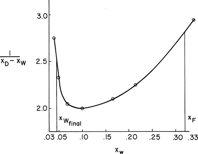
FIGURE 9-7. Graphical integration, Example 9-2
Then from Eq. (9-7),
Wfinal = Fe–Area = (50)exp(–0.608) = 27.21
From Eq. (9-8a),
Dtotal = F – Wfinal = 22.79
and from Eq. (9-8b),
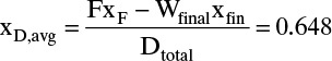
The area can also be determined by Simpson’s rule. However, because of the shape of the curve in Figure 9-7, it will be less accurate than in Example 9-1 unless the area is split into two or more parts. Simpson’s rule gives
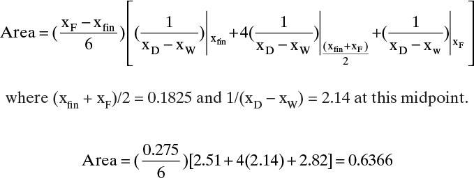
This can be checked by breaking the area into two parts and using Simpson’s rule for each part. Do one part from xfin = 0.045 to xW = 0.10 and the other part from 0.1 to xF = 0.32. Each of the two parts should fit relatively well with a cubic. Then
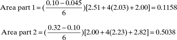
Total area = 0.6196
Note that Figure 9-7 is very useful for finding the values of 1/(xD – xW) at the intermediate points xW = 0.0725 (value = 2.03) and xW = 0.21 (value = 2.23). The total area calculated is closer to the answer obtained graphically (1.9% difference compared to 4.7% difference for the first estimate).
Then doing the same calculations as previously [Eqs. (9-7), (9-8a), and (9-8b)] with Area = 0.6196,
E. Check. The mass balances for an entire cycle, Eqs. (9-1) and (9-2), should be and are satisfied. Since the graphical integration and Simpson’s rule (done as two parts) give similar results, this is another reassurance.
F. Generalize. Note that we did not need to find the exact value of xD that corresponds to xF or xfin. We just made sure that our calculated values went beyond these values and then used Figure 9-7 to interpolate to find values for Simpson’s rule. This is true for both integration methods. Our axes in Figure 9-7 were selected to give maximum accuracy; thus, we did not graph parts of the diagram that we did not use. The same general idea applies if fitting data—fit the data only in the region needed. For more accuracy, Figure 9-6 should be expanded. If Simpson’s rule is to be used for very sharply changing curves or curves with maxima or minima, accuracy is better if the curve is split into two or more parts. Comparison of the results obtained with graphical integration to those obtained with the two-part integration with Simpson’s rule shows a difference in xD,avg of 0.008. This is within the accuracy of the equilibrium data.
Once xfin, D, and Wfinal are determined, we can calculate the values of Qc, QR, and operating time (see Section 9.8).
9.6.2 Variable Reflux Ratio
Batch distillation columns can also be operated with a variable reflux ratio to keep xD constant. Operating Eq. (9-24) is still valid, the intersection with the y = x line will be constant at xD, but the slope varies. The McCabe-Thiele diagram for this case relating xW to xD is shown in Figure 9-8. Since xD is kept constant, the calculation procedure is simplified.
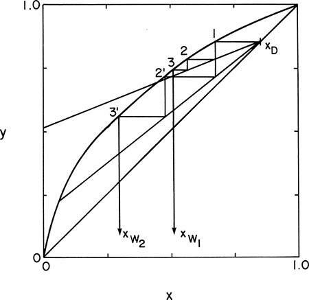
FIGURE 9-8. McCabe-Thiele diagram for multistage batch distillation with constant xD and variable reflux ratio
With xD and the number of stages specified, trial and error is required to find the initial value of L/V that gives the feed concentration xF with the specified number of stages. The operating line slope L/V is then increased until the specified number of equilibrium contacts gives xW = xfin. This gives (L/V)final. Wfinal is found from mass balance Eqs. (9-1) and (9-2).
The required maximum values of Qc and QR and the operating time can be determined next (see Section 9.8). Note that the Rayleigh equation is not required when xD is constant. However, if used, the Rayleigh equation gives exactly the same answer as Eq. (9-25) (see Problem 9.C1).
9.7 Multicomponent Simple Batch Distillation
In the derivation of the Rayleigh equation in section 9.1, we noted that the equations are valid for multicomponent mixtures. However, since the general equilibrium expression
depends on the concentration of all components, a numerical solution is required. We previously considered multicomponent simple batch distillation in section 8.5.2 when we discussed residue curves. Although the notations and the procedures are different, the developments in Sections 8.5.2 and 9.2.1 are equivalent (see Problem 9.C4). Thus, the residue curve gives us the path of the xi during the batch distillation, and from the required equilibrium calculation, it has also calculated the yi values that correspond to the xi, although the vapor values may not be reported. The profiles of xi and yi values are sufficient information to numerically integrate the Rayleigh equation.
The procedure is easiest to illustrate if the relative volatility is constant. For batch distillation the equilibrium expression, Eq. (5-28) given in Problem 5.C1, is
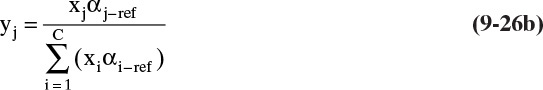
The Rayleigh equation for the light component A becomes
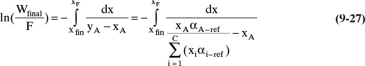
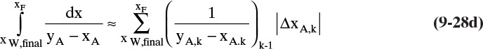
To numerically integrate the integral in Eq. (9-27), we start with the spreadsheet calculation of a residue curve (see Section 8.5.2 and Figure 8-B1). For each increment in k, the incremental area is

Then the calculated value of the integral is
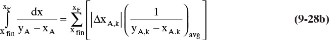
where ΔxA,k = xA,k – xA,k–1, and (1/[yA – xA])avg = 0.5[(1/[yA – xA])k-1 + (1/[yA – xA])k].
For example, if we calculate the area for k = 10 for the spreadsheet in Figure 8-B1, we have
|ΔxA,k| = |0.989960081 – 0.990021592| = 0.000061511, and
1/(yA – xA)avg = 0.5[1/(0.99617266 – 0.990021592) + 1/(0.996149968 – 0.989960081)] = 162.06.
Incremental area = (0.000061511)(162.06) = 0.009969.
If the values of h and kfinal from a residue curve calculation using the Euler method (Section 8.5.2) starting with the initial conditions of the batch distillation are available, then an estimate of the area of the integral in Eq. (9-27) is
where kfinal is the step for which xA = xA,final. This equation is useful for checking the result of a numerical integration. The rationale behind Eq. (9-28c) is explored in Problem 9.C5.
EXAMPLE 9-3. Multicomponent simple batch distillation
A simple batch distillation of the ideal system benzene (B), toluene (T), and cumene (C) is run. Charge is 1.0 kmole, and the feed is 70.0 mol% benzene, 20.0 mol% toluene, and 10.0 mol% cumene. Determine Wfinal, Dtotal, xT,fin, xC,fin, xD,B,avg, xD,T,avg, and xD,C,avg if xB,fin = 0.4. Pressure is 1.0 atm, and the relative volatilities are αBT = 2.4, αTT = 1.0, and αCT = 0.21.
Solution
A. Define. The apparatus is shown in Figure 9-1. F = 1.0 kmol, xW,B,initial = 0.70, xW,T,initial = 0.20, xW,C,initial = 0.1, and xB,fin = 0.40. Find Wfinal, Dtotal, xT,fin, xC,fin, xdist,B,avg, xdist,T,avg, and xdist,C,avg.
B. Explore. We need to find the area of the integral in Eq. (9-27) so that we can calculate Wfinal. Once the total area has been found, Wfinal is given by Eq. (9-11b). The values of xT,fin and xC,fin can be determined from the residue curve. We can then find Dtotal from the overall mass balance, and the xdist,i,avg values are determined from component mass balances.
C. Plan. To find the integral of the area in Eq. (9-27) we can use a spreadsheet to generate a residue curve starting with the initial conditions. The values of xT,fin and xC,fin are on the residue curve at the value of xB,fin. The more accurate method to calculate the area is Eq. (9-28b). Thus, we will calculate the y values from Eq. (9-28b) for every step k in the calculation of the residue curve. Then 1/(y – x)avg can be calculated for each step k, and the area of each step can be determined.
D. Do It. The spreadsheet and VBA program for the calculations is shown in this chapter’s appendix with h = 0.001. The values in the spreadsheet at xB,fin = 0.4 are found by inspecting the output manually and are shown in Table 9.1.
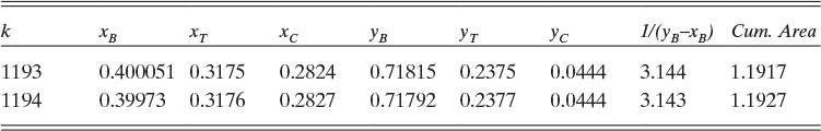
The cumulative area at xB,fin = 0.40 is approximately 1.1919.
From these results, xT,fin = 0.3175, and xC,fin = 0.2825.
Wfinal = F exp(–Area) = 1.0 exp(–1.1919) = 0.3036 kmol
Dtotal = F – Wfinal = 1 – 0.3036 = 0.6964 kmol
xB,dist,avg = [FxB,init – WfinalxB,fin]/Dtotal = [0.7 – (0.3036)(0.4)]/0.6964 = 0.8308
xT,dist,avg = [FxT,init – WfinalxT,fin]/Dtotal = [0.2 – (0.3036)(0.3175)]/0.6964 = 0.1488
xC,dist,avg = [FxC,init – WfinalxC,fin]/Dtotal = [0.1 – (0.3036)(0.2825)]/0.6964 = 0.0204
E. Check. ∑ xi,dist,avg = 1.0000 which is OK.
In addition, the approximate solution for the area, Eq. (9-28c), gives
Area = (k – 1)h = (1193 – 1)(0.001) = 1.192
which agrees with the area calculation from the spreadsheet.
F. Generalize. This method can be applied to any number of components if the relative volatilities are constant.
If the relative volatilities are not constant, we have two choices. First, we can divide the range of the batch operation into a series of intervals and use an average value ![]() for each interval. A reasonable definition of
for each interval. A reasonable definition of ![]() is the geometric average for each interval:
is the geometric average for each interval:
The recursion Eq. (8-30) uses ![]() values that correspond to the interval in which they appear.
values that correspond to the interval in which they appear.
The second procedure, which is more accurate, is to do a bubble-point calculation at every time step. The use of bubble-point calculations is explored in section 5.3 in the context of a steady-state, multistage analysis. For batch distillation the bubble-point calculation would be done at each step k. In essence, the resulting spreadsheet is a combination of the spreadsheets in Appendices 5A and 9A.
Fractions (Section 9.2.2) are often collected in multicomponent batch distillation. With only a single-stage, simple batch distillation does not give pure compounds unless the relative volatilities are very large. The calculation method is quite similar to the method shown in Example 9.3. For example, if a second fraction was collected for Example 9.3 when xW,B,2 = 0.3, we would look at the results of the spreadsheet in Appendix A to find the mole fractions and the cumulative area at this concentration. The values bracketing xW,B,2 = 0.3 are shown in Table 9.2.
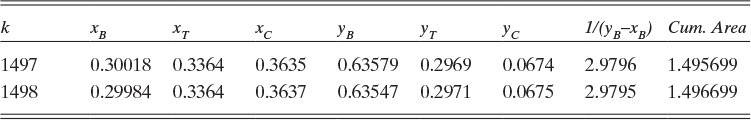
The cumulative area at xW,B,2 = 0.3 is approximately 1.4962. If we subtract this value from the cumulative area = 1.1919 at xW,B = 0.4, we determine the area for the fraction from xW,B = 0.4 to xW,B = 0.3 is 0.3043. The initial charge for this fraction was Wfinal = 0.3036 calculated in Example 9.3. Then W(at xW,B = 0.3) = (0.3036)exp(–0.3043) = 0.2239 kmole. (See Problem 9.D27a for an equivalent calculation and Problem 9.D27b for the completion of the problem.)
Obviously, multistage batch columns are also used for multicomponent separations. One fairly simple approach is to assume that the changes in the column are quite slow and use a steady-state analysis similar to that employed in Section 9.6 for binary separations. Examples are the Fenske-Underwood-Gilliland shortcut method or stage-by-stage calculation with bubble-point calculation on each stage. Since these analyses ignore holdup on the stages and dynamics of the stages, they are considered simple models. More complicated models include stage holdup and dynamics and may include a mass transfer analysis. Readers interested in these more advanced topics should consult Sorensen (2014) for references and Diwekar (2012) and Mujtaba (2004) for calculation details.
9.8 Operating Time
Operating time and batch size may be controlled by economics or other factors. For instance, it is not uncommon for the entire batch including startup and shutdown to be done in one 8-hour shift. If the same apparatus is used for several different chemicals, the batch sizes may vary. In addition, the time to change over from one chemical to another may be quite long, since a rigorous cleaning procedure may be required.
The total batch time, tbatch, is
The down time, tdown, includes dumping the bottoms, cleanup, loading the next batch, and heating the next batch until reflux starts to appear. This time can be estimated from experience. The operating time, top, is the actual period during which distillation occurs, so it must be equal to the total amount of distillate collected divided by the distillate flow rate.
Dtotal is calculated from the Rayleigh equation, with F set either by the size of the still pot or by the charge size. For an existing apparatus the distillate flow rate, D in kmol/h, cannot be set arbitrarily. The column was designed for a given maximum vapor velocity, uflood, which corresponds to a maximum molal flow rate, Vmax (see Chapter 10). Then from the mass balance around the condenser,
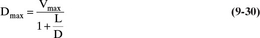
We usually operate at a fraction of the maximum flow rate, such as D = 0.75 Dmax. The operating time, top, can be estimated from Eqs. (9-29) and (9-30). If the resulting tbatch is not convenient, adjustments must be made.
The energy requirements in the reboiler or still pot, QR, and in the total condenser, Qc, can be estimated from energy balances. For a total condenser Eq. (3-13) is valid, but V1, hD, and H1 may all be functions of time (if xD varies, the enthalpies will vary). If the reflux is a saturated liquid reflux, then H1 – hD = λ, the latent heat of evaporation. In this case the total condenser just condenses the vapor to saturated liquid. Likewise, the still pot vaporizes a saturated liquid to a vapor. Thus,
If CMO is valid, then V1 = Vpot, λ1 = λpot, and
Since V = (1 + L/D)D, we obtain
For an existing batch distillation apparatus we must check that the condenser and the reboiler are large enough to handle the calculated values of |Qc| and QR. If |Qc| or QR is too large, then the rate of vaporization needs to be decreased. Either the operating time, top, will need to be increased or the charge to the still pot F will have to be decreased.
During operation (assume that the charge and the still pot have been heated and vapor is flowing throughout the column), the energy balance around the entire system is
If CMO is valid, Eq. (9-31c) holds, and saturated liquid hD = hpot, the result simplifies to
If the assumption of negligible holdup is not valid, then the holdup on each stage and in the accumulator acts like a flywheel and retards changes. A different calculation procedure is required for this case (Diwekar, 2012; Mujtaba, 2004). Batch distillation also has somewhat different design and process control requirements than continuous distillation. In addition, startup and troubleshooting are somewhat different (Sorensen, 2014).
References
Carey, J. S., “Distillation,” in J. H. Perry (Ed.), Chemical Engineer’s Handbook, 3rd ed., McGraw-Hill, New York, 1950, pp. 582–585.
Davies, J. T., “Chemical Engineering: How Did It Begin and Develop?” in W. F. Furter (Ed.), History of Chemical Engineering, Washington, D.C., American Chemical Society, Adv. Chem. Ser, 190, 15–43 (1980).
Diwekar, U. W., Batch Distillation: Simulation, Optimal Design and Control, 2nd ed., Taylor and Francis, Washington, D.C., 2012.
Gentilcore, M. J., “Reduce Solvent Usage in Batch Distillation,” Chem. Engr. Progress, 98 (1), 56 (Jan. 2002).
Kockmann, N., “History of Distillation,” in Gorak, A., and E. Sorensen (Eds.), Distillation: Fundamentals and Principles, Chapter 1, Elsevier, 2014.
Larsson, L., R. E. Eliasson, and M. Orych, Principles of Yacht Design, 4th ed., International Marine/McGraw-Hill Education, Camden, Maine, 2014. [Note: An unusual reference in a chemical engineering textbook; however, mathematics is universally applicable. Their description of Simpson’s rule with examples is clear.]
Luyben, W. L., “Some Practical Aspects of Optimal Batch Distillation,” Ind. Eng. Chem. Process Des. Develop., 10, 54 (1971).
Mujtaba, I. M., Batch Distillation: Design and Operation, Imperial College Press, London, 2004.
Mickley, H. S., T. K. Sherwood, and C. E. Reed, Applied Mathematics in Chemical Engineering, McGraw-Hill, New York, 1957, pp. 35–42.
Pratap, R., Getting Started with MATLAB7, Oxford University Press, Oxford, 2006.
Pratt, H. R. C., Countercurrent Separation Processes, Elsevier, New York, 1967.
Rayleigh, Lord (J. Strutt), “On the Distillation of Binary Mixtures,” Phil. Mag. [VI], 4 (23), 521 (1902).
Robinson, C. S., and E. R. Gilliland, Elements of Fractional Distillation, 4th ed., McGraw-Hill, New York, 1950, Chapters 6 and 16.
R. T., “Distillation through the Ages,” Chem. Heritage, 25 (2), 40 (Summer 2007).
Sorensen, E., “Design and Operation of Batch Distillation,” in Gorak, A., and E. Sorensen (Eds.), Distillation: Fundamentals and Principles, Chapter 5, Elsevier, London, UK, 2014.
Stanwood, C., “Found in the Othmer Library,” Chemical Heritage, 23 (3), 34 (Fall 2005).
Treybal, R. E., Mass-Transfer Operations, 3rd ed., McGraw-Hill, New York, 1980.
Treybal, R. E., “A Simple Method for Batch Distillation,” Chem. Eng., 77 (21), 95 (Oct. 5, 1970).
Vallee, B. L., “Alcohol in the Western World,” Scientific American, 80 (June 1998).
Woodland, L. R., “Steam Distillation,” in D. J. DeRenzo (Ed.), Unit Operations for Treatment of Hazardous Industrial Wastes, Noyes Data Corp., Park Ridge, NJ, 1978, pp. 849–868.
Homework
A. Discussion Problems
A1. Why is the still pot in Figure 9-2B much larger than the column?
A2. In the derivation of the Rayleigh equation:
a. In Eq. (9-4), why do we have –xD dW instead of –xD dD?
b. In Eq. (9-4), why is the left-hand side –xD dW instead of –d(xDW)?
A3. Explain how the graphical integration shown in Figures 9-3 and 9-5 could be done numerically on a computer.
A4. Suppose you have two feeds containing methanol and water that you want to batch distil. One feed is 60.0 mol% methanol, and the other is 32.0 mol% methanol. How do you do the batch distillation to obtain the largest amount of distillate of a given mole fraction? N is constant.
a. Mix the two feeds together and batch distil.
b. Start the batch with the feed with higher methanol mole fraction and then add second feed (32.0 mol% methanol) when the still-pot concentration equals that feed concentration.
c. Do two separate batches—one for the more concentrated feed (60.0 mol%) and the other for the less concentrated feed (32.0 mol%).
d. All of the above.
e. a and b.
f. a and c.
g. b and c.
h. None of the above.
Explain your answer.
A5. Which system(s) require less energy for batch distillation than continuous distillation with the same amount of separation?
a. Simple batch compared to one-stage continuous.
b. Multistage batch compared to multistage continuous.
c. Batch steam distillation compared to continuous steam distillation.
d. All of the above.
e. a and b.
f. a and c.
g. b and c.
h. None of the above.
Explain your answer.
A6. Batch-by-Night, Inc., has developed a new simple batch with reflux system (Figure 9-1 with some of stream D refluxed to the still pot) that they claim outperforms the normal simple batch (Figure 9-1). Suppose you want to batch distil a mixture similar to methanol and water in which there is no azeotrope and two liquid phases are not formed. Both systems are loaded with the same charge F moles with the same mole fraction xF, and distillation is done to the same value xw,final. Will the value of xd,avg from the simple batch with reflux be
a. greater than
b. the same as
c. less than
the xd,avg value from the normal, simple batch distillation? Explain your answer.
A7. When there are multiple stages in batch distillation, the calculation looks like the McCabe-Thiele diagram for several
a. stripping columns.
b. enriching columns.
c. columns with a feed at the optimum location.
A8. Develop a key relations chart for this chapter.
A9. If we are doing a batch distillation of a heterogeneous azeotrope system, when would we employ a system similar to Figure 9-1, and when would we employ a system similar to Figure 9-10 (in Problem 9.D9)?
B. Generation of Alternatives
B1. List all the different ways a binary batch or inverted batch problem can be specified. Which of these will be trial and error?
B2. What can be done if an existing batch system cannot produce the desired values of xD and xW even at total reflux? Generate ideas for both operating and equipment changes.
B3. Develop ideas for how you would reprocess or utilize the offcuts from a batch distillation that collects fractions.
C. Derivations
C1. For a binary multistage batch distillation with constant xdist, prove that the mass balances over the entire batch period and the Raleigh equation both give Eq. (9-25).
C2. Assume that holdup in the column and in the total reboiler is negligible in an inverted batch distillation (Figure 9-9).
a.* Derive the appropriate form of the Rayleigh equation.
b. Derive the necessary operating equations for CMO. Sketch the McCabe-Thiele diagrams.
C3. If relative volatility can be assumed constant over the change in concentration for each fraction, Eq. (9-13) can be adapted to the collection of fractions from a simple binary batch distillation. Derive the equations for a simple batch with three distillate fractions collected.
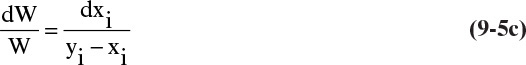
C4. Show that Eq. (9-5c) [immediately before Eq. (9-14)] is equivalent to Eq. (8-27c).
C5. If we approximate the area in Eq. (9-28b) as
then the incremental area for k = 10 (see the section immediately before Example 9.3) = (0.000061511)(162.573393759) = 0.01000005 = h = 0.01. From this result, you can deduce the approximate Eq. (9-28c).
a. Prove that this agreement of the numerical value of the estimated incremental area and the value of h is not an accident.
b. Explain how Eq. (9-28c) can be deduced.
c. Check the prediction of Eq. (9-28c) for Example 9.3.
D. Problems
*Answers to problems with an asterisk are at the back of the book.
D1. A simple batch distillation separates 0.6 kmol of a binary feed that is 70.0 mol% methanol and 30.0 mol% water. The final still pot is 10.0 mol% methanol. Find Wfinal, distillate Dtotal, and xD,avg. VLE data are in Table 2-7. p = 1.0 atm.
D2.* A simple batch still (one equilibrium stage) separates 100 moles of a 75.0 mol% methanol and 25.0 mol% water feed. The final bottoms concentration is 55.0 mol% methanol. Find Wfinal, distillate Dtotal, and xD,avg. VLE data are in Table 2-7. p = 1.0 atm.
D3.* A distillation system with a still pot plus a column with one equilibrium stage is used to batch distil 1.0 kmol of a 57.0 mol% methanol and 43.0 mol% water feed. A total condenser is used. The final bottoms concentration is 15.0 mol% methanol. Pressure is 101.3 kPa. Reflux is a saturated liquid, and L0/D = 1.85. Find Wfinal, Dtotal, and xD,avg. VLE data are in Table 2-7.
D4. A simple batch distillation (one equilibrium contact) is done of an 80.0 mol% acetone and 20.0 mol% ethanol feed. The final concentration in the still pot is 40.0 mol% acetone, and Wfinal = 2.0 kmole. VLE data are in Problem 4.D7. Find the feed amount F, the average mole fraction of the distillate, and the kmoles of distillate Dtotal collected.
D5. 3.0 kmol of feed containing 52.0 mol% water and 48.0 mol% n-butanol is charged to the still pot of a simple batch distillation system (Figure 9-1). The final still pot concentration should be 28.0 mol% water. Equilibrium data are in Table 8-2.
a. Find Wfinal (kmole), DV,tot (total amount of distillate vapor collected, kmole), and yD,avg (average mole fraction water in the vapor distillate).
b. After the distillate vapor is condensed in the total condenser, the liquid is sent to a liquid-liquid settler. Find the total amount of each distillate liquid collected, D1 (with xD1,water = 0.573) and D2 (with xD2,water = 0.975), in kmoles.
D6. A simple batch still separating a feed that is 60.0 mol% 1,2 dichloroethane and 40.0 mol% 1,1,2-trichloroethane. Pressure is 1 atm. The relative volatility is constant, αdi-tri = 2.4. The use of Eq. (9-13) is recommended.
a. The charge (F) is 1.3 kmol. The final still pot concentration is 30.0 mol% 1,2 dichloroethane. Find the final moles in still pot and the average mole fraction of distillate product.
b. Repeat part a if F = 3.5 kmol.
c. If F = 2.0 kmol and the average distillate concentration is 75.0 mol% 1,2-dicholoroethane, find final kmoles in the still pot and the final mole fraction of 1,2 dichloroethane in the still pot.
D7. A batch distillation system with a still pot and one equilibrium stage (two equilibrium contacts total) distills a feed that is 10.0 mol% water and 90.0 mol% n-butanol (see Table 8-2 for VLE data). p = 1.0 atm. The charge is 4.0 kmoles. The final still concentration is 2.0 mol% water. The system has a total condenser, and the reflux is a saturated liquid. L/D = 1/2. Find the final number of moles in the still pot and the average concentration of distillate.
D8. 10.0 kmol of a feed with xF = 0.4 (mole fraction methanol) and the remainder water is sent to a batch distillation system with a large still pot that is an equilibrium contact, a distillation column that acts as two equilibrium contacts (total three equilibrium contacts), and a total condenser. p = 1.0 atm. We operate with a constant xD = 0.8 as we increase L/D. The batch operation is continued until L/D = 4.0. CMO is valid. VLE data are in Table 2-7. Find:
a. xw,final.
b. Wfinal and Dtotal.
c. Initial L/D.
D9.* We wish to batch distil a mixture of 1-butanol and water. Since this system has a heterogeneous azeotrope (see Chapter 8), we will use the system shown in Figure 9-10. The bottom liquid layer from the liquid-liquid separator (97.5 mol% water) is removed as product, and the top liquid layer (57.3 mol% water) is returned to the still pot. Pressure is 1 atm. The feed is 20.0 kmol and 40.0 mol% water. Data are given in Problem 8.D2.
a. If the final concentration in the still pot is xW,final = 0.28, find Dtotal in kmoles.
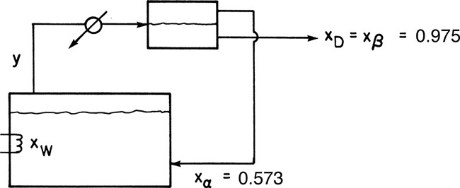
b. If the batch distillation is continued what is the lowest value of xW,final that can be obtained while still producing a distillate xD = 0.975?
D10. 4.0 kmoles of a feed that is 0.60 mole fraction acetone and 0.40 mole fraction ethanol is batch distilled in a system with a still pot (an equilibrium contact), a column that acts as one equilibrium stage (total two equilibrium contacts), a total condenser, and reflux to the column. p = 1.0 atm, the reflux ratio is L/D = 1.0, CMO is valid, and xW,final = 0.20. VLE data are in Problem 4.D7. Find Wfinal, xdist,avg, and Dtotal.
D11. A constant-mole batch distillation is used to change from a pure n-butanol solvent to a solvent that is 60.0 mol% n-butanol and 40.0 mol% water. If the initial charge is W = 2.0 kmol, how much water, S, must be added to achieve the desired solvent concentration? Do the integration with Simpson’s rule, dividing the entire integration from 0.6 to 1.0 first into one step and then into two steps. Compare the answers.
D12. A nonvolatile pharmaceutical is dissolved in a solution that is 90.0 mol% acetone and 10.0 mol% ethanol. A constant volume batch distillation is used to switch the solvent to 20.0 mol% acetone and 80.0 mol% ethanol without diluting the concentration of solute. The charge to the still pot is W = 1.5 kmol. VLE data are in Problem 4.D7. What are the values of the amount (kmol) of pure solvent ethanol added, the kmol of acetone that are evaporated, the kmol of ethanol evaporated, and the average mole fraction of acetone in the distillate?
D13. A simple batch distillation (Figure 9-1) is separating 8.00 kmol of a feed that is 40.0 mol% water and 60.0 mol% n-butanol. The batch distillation is continued until the still pot contains 0.080 mole fraction water. VLE data are in Table 8-2, Problem 8.D3.
a. Find Wfinal, Dtotal, and xD,avg.
b. After settling, the final distillate product is two liquid phases. What are the mole fractions and the amounts (kmol) of each liquid phase?
Note: Problem 9.D28 shows that Figure 9-10 gives a better separation.
D14.* A simple steam distillation is being done in the apparatus shown in Figure 9-5. The organic feed is 90.0 mol% n-decane and 10.0% nonvolatile organics. The system is operated with liquid water in the still. Distillation is continued until the organic layer in the still is 10.0 mol% n-decane. F = 10 kmole. Pressure is 760 mm Hg.
a. At the final time, what is the temperature in the still?
b. What are values of Wfinal and Dtotal?
c. Estimate the moles of water passed overhead per mole of n-decane at the end of the distillation.
Data: Assume that water and n-decane are completely immiscible. Vapor pressure data for nC10 are in Example 8-2. Vapor pressure data for water are listed in Problem 8.D10.
D15. 12.0 kmole of a mixture 0.40 mole fraction water and 0.60 mole fraction n-butanol at 1.0 atm pressure is batch distilled in a system with an equilibrium still pot and a column with one equilibrium stage (total two equilibrium contacts). Vapor from the column is sent to a total condenser and then to a liquid-liquid settler. The aqueous phase from the settler (0.975 mole fraction water) is removed as the distillate product. The organic phase from the settler (0.573 mole fraction water) is refluxed to the distillation column. (The equipment is a modification of Figure 9-10 with a column between the still pot and the condenser.) Dtotal = 3.9 kmol. Equilibrium data are in Table 8-2 (in Problem 8.D3).
a. Find Wfinal and xW,final.
b. Find the approximate value of the reflux ratio L/D at end of the batch distillation.
D16.* 10.0 kmol of a 40.0 mol% methanol and 60.0 mol% water mixture is processed in a normal batch distillation system with a still pot that acts as an equilibrium stage and a column with two equilibrium stages (total of three equilibrium contacts). The column has a total condenser, and reflux is a saturated liquid. The column is operated with a varying reflux ratio so that xD is held constant. We desire a final still-pot concentration of 8.0 mol% methanol, and distillate should be 84.0 mol% methanol. Pressure is 1 atm, and CMO is valid.
a. What initial external reflux ratio, L0/D, must be used?
b. What final external reflux ratio must be used?
c. How much distillate product is withdrawn, and what is the value of Wfinal?
D17. A nonvolatile solute is dissolved in 1.0 kmol of methanol. We wish to have the solute in 1.0 kmol of solution that is 99.0 mol% water and 1.0 mol% methanol. Because the solution is already concentrated, a first batch distillation to concentrate the solution is not required. VLE data (ignore the effect of the solute) are in Table 2-7. Do a constant-mole batch distillation from xM,initial = 1.0 (pure methanol) to xM,final = 0.01. Find the moles of water added during the constant-mole batch distillation and the moles of water evaporated with the methanol in the distillate. Results can be compared with dilution followed by simple batch distillation in Problem 9.E4.
Note: Since xM,final = 0.01 is quite small, 1/y is quite large at this limit. To use Simpson’s rule divide the integral into at least two sections.
D18. A differential condensation [see Eq. (9-14)] is done for a binary mixture of ethanol and water. The feed is 0.50 kmol of vapor that is 0.10 mole fraction ethanol. The differential condensation is continued until the vapor remaining is yD,final = 0.50 mole fraction ethanol. Find the values of Dfinal and the condensate Ctotal and the average mole fraction of ethanol in the condensate, xC,avg. Note that this operation can only be approximated in practice (Treybal, 1980). Compare the result to the solution to Problem 9.D1.
D19. Batch steam distillation is being done to recover octanol from nonvolatile organics. Assume that water and octanol, and water and the nonvolatile organics are completely immiscible. The water layer is pure. The organic layer in the still pot contains 0.60 mole fraction octanol and 0.40 mole fraction nonvolatile organics. The still pot temperature is 90.0°C. The Antoine equations (T is in °C, and VP is the vapor pressure in mm Hg) are:
Octanol: log10 (VP) = 6.8379 – 1310.62/(T + 135.05)
Water: log10 (VP) = 8.68105 – 2164.42/(T + 273.16)
What is the pressure of the still pot?
D20. 10.0 kmole of a 40.0 mol% methanol and 60.0 mol% water mixture is batch distilled. The system consists of a column with two equilibrium stages, a still pot (an equilibrium contact), and a total condenser. The system is operated with a reflux ratio L/D = 0.515. The final concentration of methanol in the still pot is xW,final = 0.075. CMO is valid. If you use Simpson’s rule, break the area into at least two parts. Find Wfinal, Dtotal, and xdist,avg.
D21. Repeat Problem 9.D20 but for a distillation column with 20 stages.
Note: Think smart and this problem is significantly less work than Problem 9.D20.
D22. 3.0 kmol of a 62.0 mol% methanol and 38.0 mol% water are batch distilled in a system with a still pot and a column with one equilibrium stage (two equilibrium contacts total). Distillate concentration is constant at 85.0 mol% methanol. The final still pot concentration is 45.0 mol% methanol. Reflux is a saturated liquid, and L/D varies. Assume CMO.
a. Find Dtotal and Wfinal (kmoles).
b. Find the final value of the external reflux ratio L/D.
D23.* 1.2 kmol of a 10.0 mol% ethanol and 90.0 mol% water feed is processed in a simple batch distillation system that consists of a still pot, a total condenser, and a fraction collector. We collect three fractions with xW1 = 7.0 mol% ethanol, xW2 = 4.0 mol% ethanol, and xW3 = xW,final = 1.0 mol% ethanol. Find W1, W2, and Wfinal; D1, D2, and D3 in kmole; and mole fractions of ethanol xD1,avg, xD2,avg, and xD3,avg. p = 1.0 atm.
D24. A constant-mole batch distillation is being done to replace methanol with water as solvent for a nonvolatile solute currently dissolved in methanol. The system has a still pot and a condenser and operates with no reflux. The initial state has Winitial = 10.0 kmol, and xw,MeOH,initial = 1.00. The final state has Wfinal = 10.0 kmol, xw,MeOH,final = 0.10, and xw,water,final = 0.90 mole fraction. Pressure = 1.0 atm.
a. Find S, the kmol of water added, and Dtotal = kmol of distillate.
b. Find the average distillate mole fraction of methanol, xdist,MeOH,avg.
c. If the heating rate is constant at 100 kW, how many hours does the constant mole batch distillation require (assume water is added as a saturated liquid)?
D25. 1.5 kmol of feed one that is 40.0 mol% methanol and 60.0 mol% water and 1.0 kmol of feed two that is 20.0 mol% methanol and 80.0 mol% water will be processed in a simple batch distillation. The following three approaches have been proposed:
a. Mix the two feeds together, and do the batch distillation.
b. Do a batch distillation of feed one until the still pot concentration is 20 mol% methanol (same as feed two), add feed two, and then complete the batch distillation.
c. Do a batch distillation of feed one and a separate batch distillation of feed two. Add the two distillate products and the two still-pot products.
If we want xW,final,total = 0.10, do calculations for each method. Determine Wfinal, Dtotal, and xD,average, and compare the three methods. Equilibrium data are in Table 2-7. Logically, parts b and c should give the same result. If they do not, there is probably a numerical error from the use of Simpson’s rule. Try dividing an area into two parts for more accuracy.
D26. In Problem 9.D23 fractions were collected from ethanol mole fractions xF = 0.10 to xW1 = 0.07, from xW1 to xW2 = 0.04, and from xW2 to xW3 = xW,final = 0.01. The solution is given under Answers to Selected Problems. Now collect a first product fraction (A) from xF = 0.10 to xWA = 0.085, a second product fraction (B) from xWOC1 = 0.07 to xWB = 0.05, and a third product fraction (C), which is identical to the current fraction, 3. To obtain these product fractions we need two offcuts: OC1 from xWA = 0.085 to xWOC1 = 0.07, and OC2 from xWB = 0.05 to xWOC2 = 0.04.
a. Find W and D (in kmol) and the mole fractions of ethanol xD,avg for each fraction.
b. How would you reprocess the offcuts in the next batch?
D27. The continuation of Example 9.3 in Table 9.2 looks at removing a second fraction with xW,A,2 = 0.30.
a. An alternative equivalent calculation is to use the entire cumulative area and the original feed F = 1 kmole. Show that this alternate calculation of W(at xW,benzene = 0.30) gives the same result.
b. When xW,benzene = 0.30, what are the values of xW,toluene and xW,cumene?
c. For the fraction collected from xW,benzene = 0.40 to xW,benzene = 0.30, determine the values of Dtotal, xD,benzene,avg, xD,toluene,avg, and xD,cumene,avg.
D28. Repeat Problem 9.D13 except use Figure 9-10 as long as the distillate is in the two-phase region and then convert to simple batch distillation by bypassing the liquid-liquid settler. Compare the amounts and concentrations of the three products to Problem 9.D13.
D29. A 10.0 mol% ethanol 90.0 mol% water feed is batch distilled at 1.0 atm. The batch distillation system consists of a still pot plus a column with the equivalent of nine equilibrium contacts and a total condenser. External reflux ratio = 2/3. The initial charge to the still pot is 1000.0 kg. The final still pot concentration is 0.004 mole fraction ethanol. Find Wfinal, Dtotal, and xD,avg. Note: Stepping off ten stages for a number of operating lines sounds like a lot of work. However, after you try it once, you will notice that there is a shortcut to determining a relationship between xD and xW.
E. More Complex Problems
E1. We are doing a single-stage, batch steam distillation of 1-octanol. The unit operates at 760 mm Hg. The batch steam distillation is operated with liquid water present. The distillate vapor is condensed, and two immiscible liquid layers form. The feed is 90.0 mol% octanol, and the rest is nonvolatile organic compounds. The feed is 1.0 kmol. We desire to recover 95% of the octanol. Vapor pressure data for water are given in Problem 8.D15. For small ranges in temperature, these data can be fit to an Antoine equation form with C = 273.16. The vapor pressure equation for 1-octanol is in Problem 8.D11.
a. Find the operating temperature of the still at the beginning and end of the batch.
b. Find the amount of organics left in the still pot at the end of the batch.
c. Find the kmoles of octanol recovered in the distillate.
d. Find the kmoles of water condensed in the distillate product. To do this, use the average still temperature to estimate the average octanol vapor pressure, which can be assumed to be constant. To numerically integrate Eq. (9-23b) relate xorg to norg with a mass balance around the batch still.
e. Compare with your answer to Problem 8.D11. Which system produces more water in the distillate? Why?
E2. We wish to use batch steam distillation at 1.0 atm to recover 1-octanol from 100.0 kg of a mixture that is 15.0 wt% 1-octanol, and the remainder consists of nonvolatile organics and solids of unknown composition. The still pot is operated with liquid water in the pot. Assume the still pot is well mixed and liquid and vapor are in equilibrium. Ninety-five percent of the 1-octanol should be recovered in the distillate. Assume that water is completely immiscible with 1-octanol and with the nonvolatile organics. Because the composition of the nonvolatile organics is not known, we do a simple experiment and boil the feed mixture under a vacuum with no water present. The result is that at 0.05 atm pressure, the mixture boils at 129.8°C.
a. Find the mole fraction of 1-octanol in the feed and the effective average molecular weight of the nonvolatile organics and the solids. (Note: This is identical to the solution of part a in Problem 8.D15.)
b. Find the kg and kmole of 1-octanol in the distillate, the kg of total organics in the waste, and the 1-octanol weight fraction and the 1-octanol mole fraction in the waste.
e. Find the initial and final values of the temperature and of VPoctanol in the still pot. A spreadsheet or MATLAB is highly recommended for finding T and VP.
d. Find the kg and kmole of water in the distillate. This requires a numerical integration of Eq. (9-23b); however, the problem is simplified in this case. Because the still-pot temperature does not change much, the value of (VP)octanol is very close to constant, and the average value can be used.
e. Compare the solution with the solution of Problem 8.D15. Why does batch steam distillation require less steam than continuous steam distillation?
Octanol boils at about 195°C. The formula for octanol is CH3(CH2)6CH2OH, and its molecular weight is 130.23. Vapor pressure formulas for octanol and water are available in Problems 8.D11 and 8.D15, respectively.
E3. In inverted batch distillation the charge of feed is placed in the accumulator at the top of the column (Figure 9-9). Liquid is fed to the top of the column. At the bottom of the column bottoms are continuously withdrawn, and part of the stream is sent to a total reboiler, vaporized, and sent back up the column. During the course of the batch distillation, the less volatile component (LVC) is slowly removed from the liquid in the accumulator, and the mole fraction MVC xd increases. Assuming that holdup in the total reboiler, the total condenser, and the trays is small compared to the holdup in the accumulator, the Rayleigh equation for inverted batch distillation is
ln (Dfinal /F) = – xfeed∫xd,final [(dxd)/(xd – xB)]
We feed the inverted batch system shown in Figure 9-9 with F = 10.0 mole of a feed that is 50.0 mol% ethanol and 50.0 mol% water. We desire a final distillate mole fraction of 0.63. There are two equilibrium stages in the column. The total reboiler, the total condenser, and the accumulator are not equilibrium contacts. VLE data are in Table 2-1. Find Dfinal, Btotal, and xB,avg if the boilup ratio is 1.0.
E4. A nonvolatile solute is dissolved in 1.0 kmol of methanol. We wish to switch the solvent to water. Because the solution is already concentrated, a first batch distillation to concentrate the solution is not required. We desire to have the solute in 1.0 kmol of solution that is 99.0 mol% water and 1.0 mol% methanol. This can be done either with a constant-mole batch distillation or by diluting the mixture with water and then doing a simple batch distillation. VLE data (ignore the effect of the solute) are in Table 2-7. Dilute the original pure methanol (plus solute) with water and then do a simple batch distillation with the goal of having Wfinal = 1.0 and xM,final = 0.01. Find the moles of water added and the moles of water evaporated during the batch distillation. Compare with the constant-mole batch distillation in Problem 9.D17.
E5. A simple batch distillation is used to process 1.0 kmole of methanol-water feed into three distillate fractions and a waste. The initial feed has xF,methanol = 0.50 mole fraction. We want the average mole fractions of methanol in the distillate fractions to be xdist,avg,1 = 0.70, xdist,avg,2 = 0.60, and xdist,avg,3 = 0.40. Equilibrium data is in Table 2-7.
Part a. Find W1,final, Dtotal,1, xW,final,1; W2,final, Dtotal,2, xWfinal,2; and W3,final, Dtotal,3, xW,final,3.
To make this problem tractable, the following procedure is suggested: Calculate relative volatility values ![]() from equilibrium data at xM = 0.5, 0.4, 0.3, 0.2, 0.15, and 0.10. Over the different ranges of still pot mole fractions expected, calculate geometric average
from equilibrium data at xM = 0.5, 0.4, 0.3, 0.2, 0.15, and 0.10. Over the different ranges of still pot mole fractions expected, calculate geometric average ![]() for each range.
for each range.
Solve Eq. (9-13) on a spreadsheet to calculate Wfin using the guessed value of xW,final. Calculate xD,avg for the fraction. Use Goal Seek to make diff = xD,avg,specificed – xD,avg,guess approach zero by changing the guess for xW,final. If the average value of relative volatility used was for an obviously incorrect range, insert a corrected ![]() , and repeat. Do this for each fraction.
, and repeat. Do this for each fraction.
Part b. In the lab or plant, it is easier to collect fractions based on weight or time than based on mole fraction measurements. If heating is done at a rate of 20 kW, at what time in minutes should we switch from collecting the first fraction to collecting the second fraction? Required data are available in the textbook (see Appendix D in the back of book).
E6. We are separating 100 moles of a feed that is 60.0 mol% methanol and 40.0 mol% water by batch distillation in a system with a still pot and a column that has one equilibrium contact (two equilibrium contacts total). Start the operation with a constant reflux ratio of L/D = 2/3. Operate with L/D = 2/3 until xdist = 0.70. Then keep the distillate mole fraction constant by varying L/D. When L/D = 4.0, stop the batch distillation.
a. Find xW,final.
b. Find Wfinal and Dtotal.
c. Find xD,avg.
H. Computer Spreadsheet Problems
H1. A mixture of benzene (A) and cumene (C) is to be distilled in a simple batch system. The initial charge of 5.0 kmol is 37.0 mol% benzene and 63.0 mol% cumene. At the system pressure of 1 atm and choosing cumene (C) as the reference component, the relative volatility is αA–C = 10.71. Use Eq. (9-13).
a. If FRbenzene,dist = 0.75, find xA,Wfinal, Wfinal, Dtotal, and xA,D,avg.
b. If xA,Wfinal = 0.05, find FRbenzene,dist, Wfinal, Dtotal, and xA,D,avg.
c. If FRbenzene,dist = 0.982, find xA,Wfinal, Wfinal, Dtotal, and xA,D,avg.
H2. Run a simple batch distillation of a mixture of benzene (A), xylene (B), and cumene (C). Initial charge is 5.0 kmole that is 72.0 mol% benzene, 13.0 mol% xylene, and 15.0 mol% cumene. If xA,Wfinal = 0.30, find Wfinal, xW,B, xW,C, Dtotal, xD,A,avg, xD,B,avg, and xD,C,avg. Constant relative volatilities are benzene = 2.25, toluene = 1.0, xylene = 0.33, and cumene = 0.21. Note: Toluene can be the reference component despite not being part of the mixture.
H3. Run a simple batch distillation of a mixture of benzene (A), xylene (B), and cumene (C). Initial charge is 2.7 kmole that is 64.3 mol% benzene, 11.6 mol% xylene, and 24.1 mol% cumene. If xA,D,avg = 0.800, find Wfinal, xW,A, xW,B, xW,C, Dtotal, xD,B,avg, and xD,C,avg. Constant relative volatilities are benzene = 2.25, toluene = 1.0, xylene = 0.33, and cumene = 0.21. Note: Toluene can be the reference component despite not being part of the mixture.
Chapter 9 Appendix A. Spreadsheet for Simple Multicomponent Batch Distillation, Constant Relative Volatility
The spreadsheet (Figures 9-A1 and 9-A2) does the calculations, and the VBA program (Table 9-A1) implements the counting of steps, incrementing values for the next iteration, and prints values on the spreadsheet. The calculation of the residue curve is identical to the spreadsheet in Appendix B of Chapter 8. The yi values are determined from the equilibrium relationship Eq. (9-26b), and the incremental area is found from Eq. (9-28b) at every step k. The spreadsheets are written for a generic ternary system with components A, B, and C. For Example 9-3, we identify A = benzene, B = toluene, and C = cumene.
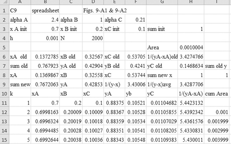
FIGURE 9-A1. Spreadsheet for multicomponent batch distillation with constant alpha showing numerical results
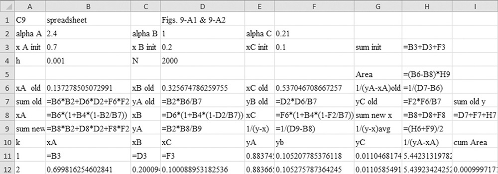
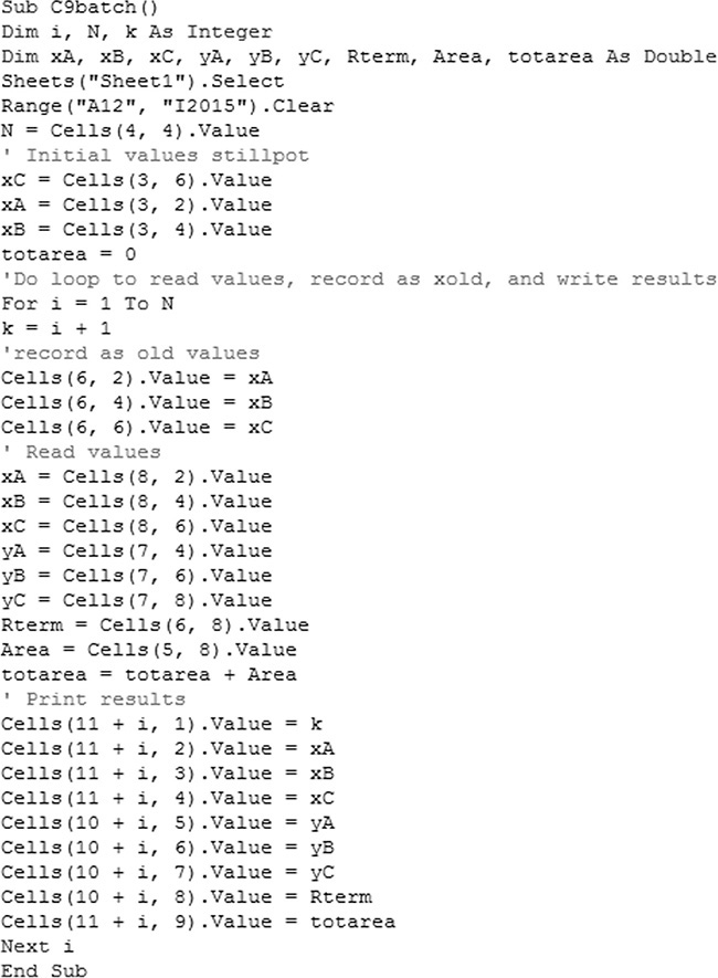
TABLE 9-A1. VBA program for spreadsheet in Figures 9-A1 and 9-A2