Chapter 7
Working with iterators and with CALCULATE
In previous chapters we provided the theoretical foundations of DAX: row context, filter context, and context transition. These are the pillars any DAX expression is built on. We already introduced iterators, and we used them in many different formulas. However, the real power of iterators starts to show when they are being used in conjunction with evaluation contexts and context transition.
In this chapter we take iterators to the next level, by describing the most common uses of iterators and by introducing many new iterators. Learning how to leverage iterators in your code is an important skill to acquire. Indeed, using iterators and context transition together is a feature that is unique to the DAX language. In our teaching experience, students usually struggle with learning the power of iterators. But that does not mean that the use of iterators is difficult to understand. The concept of iteration is simple, as is the usage of iterators in conjunction with context transition. What is hard is realizing that the solution to a complex calculation is resorting to an iteration. For this reason, we provide several examples of calculations that are simple to create with the help of iterators.
Using iterators
Most iterators accept at least two parameters: the table to iterate and an expression that the iterator evaluates on a row-by-row basis, in the row context generated during the iteration. A simple expression using SUMX will support our explanation:
Sales Amount :=
SUMX (
    Sales,                               -- Table to iterate
    Sales[Quantity] * Sales[Net Price]   -- Expression to evaluate row by row
)
SUMX iterates the Sales table, and for each row it computes the expression by multiplying quantity by net price. Iterators differ from one another in the use they make of the partial results gathered during the iteration. SUMX is a simple iterator that aggregates these results using sum.
It is important to understand the difference between the two parameters. The first argument is the value resulting from a table expression to iterate. Being a value parameter, it is evaluated before the iteration starts. The second parameter, on the other hand, is an expression that is not evaluated before the execution of SUMX. Instead, the iterator evaluates the expression in the row context of the iteration. The official Microsoft documentation does not provide an accurate classification of the iterator functions. More specifically, it does not indicate which parameters represent a value and which parameters represent an expression evaluated during the iteration. On https://dax.guide all the functions that evaluate an expression in a row context have a special marker (ROW CONTEXT) to identify the argument executed in a row context. Any function that has an argument marked with ROW CONTEXT is an iterator.
Several iterators accept additional arguments after the first two. For example, RANKX is an iterator that accepts many arguments, whereas SUMX, AVERAGEX and simple iterators only use two arguments. In this chapter we describe many iterators individually. But first, we go deeper on a few important aspects of iterators.
Understanding iterator cardinality
The first important concept to understand about iterators is the iterator cardinality. The cardinality of an iterator is the number of rows being iterated. For example, in the following iteration if Sales has one million rows, then the cardinality is one million:
Sales Amount :=
SUMX (
    Sales,                              -- Sales has 1M rows, as a consequence
    Sales[Quantity] * Sales[Net Price]  -- the expression is evaluated one million times
)
When speaking about cardinality, we seldom use numbers. In fact, the cardinality of the previous example depends on the number of rows of the Sales table. Thus, we prefer to say that the cardinality of the iterator is the same as the cardinality of Sales. The more rows in Sales, the higher the number of iterated rows.
In the presence of nested iterators, the resulting cardinality is a combination of the cardinality of the two iterators—up to the product of the two original tables. For example, consider the following formula:
Sales at List Price 1 :=
SUMX (
    'Product',
    SUMX (
        RELATEDTABLE ( Sales ),
        'Product'[Unit Price] * Sales[Quantity]
    )
)
In this example there are two iterators. The outer iterates Product. As such, its cardinality is the cardinality of Product. Then for each product the inner iteration scans the Sales table, limiting its iteration to the rows in Sales that have a relationship with the given product. In this case, because each row in Sales is pertinent to only one product, the full cardinality is the cardinality of Sales. If the inner table expression is not related to the outer table expression, then the cardinality becomes much higher. For example, consider the following code. It computes the same value as the previous code, but instead of relying on relationships, it uses an IF function to filter the sales of the current product:
Sales at List Price High Cardinality :=
SUMX (
    VALUES ( 'Product' ),
    SUMX (
        Sales,
        IF (
             Sales[ProductKey] = 'Product'[ProductKey],
             'Product'[Unit Price] * Sales[Quantity],
             0
        )
    )
)
In this example the inner SUMX always iterates over the whole Sales table, relying on the internal IF statement to check whether the product should be considered or not for the calculation. In this case, the outer SUMX has the cardinality of Product, whereas the inner SUMX has the cardinality of Sales. The cardinality of the whole expression is Product times Sales; much higher than the first example. Be mindful that this example is for educational purposes only. It would result in bad performance if one ever used such a pattern in a DAX expression.
A better way to express this code is the following:
Sales at List Price 2 :=
SUMX (
    Sales,
    RELATED ( 'Product'[Unit Price] ) * Sales[Quantity]
)
The cardinality of the entire expression is the same as in the Sales at List Price 1 measure, but the latter has a better execution plan. Indeed, it avoids nested iterators. Nested iterations mostly happen because of context transition. In fact, by looking at the following code, one might think that there are no nested iterators:
Sales at List Price 3 :=
SUMX (
    'Product',
    'Product'[Unit Price] * [Total Quantity]
)
However, inside the iteration there is a reference to a measure (Total Quantity) which we need to consider. In fact, here is the expanded definition of Total Quantity:
Total Quantity :=
SUM ( Sales[Quantity] )    -- Internally translated into SUMX ( Sales, Sales[Quantity] )

Sales at List Price 4 :=
SUMX (
    'Product',
    'Product'[Unit Price] *
        CALCULATE (
            SUMX (
                Sales,
                Sales[Quantity]
            )
        )
)
You can now see that there is a nested iteration—that is, a SUMX inside another SUMX. Moreover, the presence of CALCULATE, which performs a context transition, is also made visible.
From a performance point of view, when there are nested iterators, only the innermost iterator can be optimized with the more efficient query plan. The presence of outer iterators requires the creation of temporary tables in memory. These temporary tables store the intermediate result produced by the innermost iterator. This results in slower performance and higher memory consumption. As a consequence, nested iterators should be avoided if the cardinality of the outer iterators is very large—in the order of several million rows.
Please note that in the presence of context transition, unfolding nested iterations is not as easy as it might seem. In fact, a typical mistake is to obtain nested iterators by writing a measure that is supposed to reuse an existing measure. This could be dangerous when the existing logic of a measure is reused within an iterator. For example, consider the following calculation:
Sales at List Price 5 :=
SUMX (
    'Sales',
    RELATED ( 'Product'[Unit Price] ) * [Total Quantity]
)
The Sales at List Price 5 measure seems identical to Sales at List Price 3. Unfortunately, Sales at List Price 5 violates several of the rules of context transition outlined in Chapter 5, “Understanding CALCULATE and CALCULATETABLE”: It performs context transition on a large table (Sales), and worse, it performs context transition on a table where the rows are not guaranteed to be unique. Consequently, the formula is slow and likely to produce incorrect results.
This is not to say that nested iterations are always bad. There are various scenarios where the use of nested iterations is convenient. In fact, in the rest of this chapter we show many examples where nested iterators are a powerful tool to use.
Leveraging context transition in iterators
A calculation might require nested iterators, usually when it needs to compute a measure in different contexts. These are the scenarios where using context transition is powerful and allows for the concise, efficient writing of complex calculations.
For example, consider a measure that computes the maximum daily sales in a time period. The definition of the measure is important because it defines the granularity right away. Indeed, one needs to first compute the daily sales in the given period, then find the maximum value in the list of computed values. Even though it would seem intuitive to create a table containing daily sales and then use MAX on it, in DAX you are not required to build such a table. Instead, iterators are a convenient way of obtaining the desired result without any additional table.
The idea of the algorithm is the following:
Iterate over the Date table.
Compute the sales amount for each day.
Find the maximum of all the values computed in the previous step.
You can write this measure by using the following approach:
Max Daily Sales 1 :=
MAXX (
    'Date',
    VAR DailyTransactions =
        RELATEDTABLE ( Sales )
    VAR DailySales =
        SUMX (
            DailyTransactions,
            Sales[Quantity] * Sales[Net Price]
        )
    RETURN
        DailySales
)
However, a simpler approach is the following, which leverages the implicit context transition of the measure Sales Amount:
Sales Amount :=
SUMX (
    Sales,
    Sales[Quantity] * Sales[Net Price]
)

Max Daily Sales 2 :=
MAXX (
    'Date',
    [Sales Amount]
)
In both cases there are two nested iterators. The outer iteration happens on the Date table, which is expected to contain a few hundred rows. Moreover, each row in Date is unique. Thus, both calculations are safe and quick. The former version is more complete, as it outlines the full algorithm. On the other hand, the second version of Max Daily Sales hides many details and makes the code more readable, leveraging context transition to move the filter from Date over to Sales.
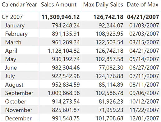
You can view the result of this measure in Figure 7-1 that shows the maximum daily sales for each month.

By leveraging context transition and an iteration, the code is usually more elegant and intuitive to write. The only issue you should be aware of is the cost involved in context transition: it is a good idea to avoid measure references in large iterators.
By looking at the report in Figure 7-1, a logical question is: When did sales hit their maximum? For example, the report is indicating that in one certain day in January 2007, Contoso sold 92,244.07 USD. But in which day did it happen? Iterators and context transition are powerful tools to answer this question. Look at the following code:
Date of Max =
VAR MaxDailySales = [Max Daily Sales]
VAR DatesWithMax =
    FILTER (
        VALUES ( 'Date'[Date] ),
        [Sales Amount] = MaxDailySales
    )
VAR Result =
    IF (
        COUNTROWS ( DatesWithMax ) = 1,
        DatesWithMax,
        BLANK ()
    )
RETURN
    Result
The formula first stores the value of the Max Daily Sales measure into a variable. Then, it creates a temporary table containing the dates where sales equals MaxDailySales. If there is only one date when this happened, then the result is the only row which passed the filter. If there are multiple dates, then the formula blanks its result, showing that a single date cannot be determined. You can look at the result of this code in Figure 7-2.
The use of iterators in DAX requires you to always define, in this order:
The granularity at which you want the calculation to happen,
The expression to evaluate at the given granularity,
The kind of aggregation to use.
In the previous example (Max Daily Sales 2) the granularity is the date, the expression is the amount of sales, and the aggregation to use is MAX. The result is the maximum daily sales.
There are several scenarios where the same pattern can be useful. Another example could be displaying the average customer sales. If you think about it in terms of iterators using the pattern described above, you obtain the following: Granularity is the individual customer, the expression to use is sales amount, and the aggregation is AVERAGE.
Once you follow this mental process, the formula is short and easy:
Avg Sales by Customer :=
AVERAGEX ( Customer, [Sales Amount] )
With this simple formula, one can easily build powerful reports like the one in Figure 7-3 that shows the average sales per customer by continent and year.

Context transition in iterators is a powerful tool. It can also be expensive, so always checking the cardinality of the outer iterator is a good practice. This will result in more efficient DAX code.
Using CONCATENATEX
In this section, we show a convenient usage of CONCATENATEX to display the filters applied to a report in a user-friendly way. Suppose you build a simple visual that shows sales sliced by year and continent, and you put it in a more complex report where the user has the option of filtering colors using a slicer. The slicer might be near the visual or it might be in a different page.
If the slicer is in a different page, then looking at the visual, it is not clear whether the numbers displayed are a subset of the whole dataset or not. In that case it would be useful to add a label to the report, showing the selection made by the user in textual form as in Figure 7-4.
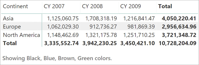
One can inspect the values of the selected colors by querying the VALUES function. Nevertheless, CONCATENATEX is required to convert the resulting table into a string. Look at the definition of the Selected Colors measure, which we used to show the colors in Figure 7-4:
Selected Colors :=
"Showing " &
CONCATENATEX (
    VALUES ( 'Product'[Color] ),
    'Product'[Color],
    ", ",
    'Product'[Color],
    ASC
) & " colors."
CONCATENATEX iterates over the values of product color and creates a string containing the list of these colors separated by a comma. As you can see, CONCATENATEX accepts multiple parameters. As usual, the first two are the table to scan and the expression to evaluate. The third parameter is the string to use as the separator between expressions. The fourth and the fifth parameters indicate the sort order and its direction (ASC or DESC).
The only drawback of this measure is that if there is no selection on the color, it produces a long list with all the colors. Moreover, in the case where there are more than five colors, the list would be too long anyway and the user experience sub-optimal. Nevertheless, it is easy to fix both problems by making the code slightly more complex to detect these situations:
Selected Colors :=
VAR Colors =
    VALUES ( 'Product'[Color] )
VAR NumOfColors =
    COUNTROWS ( Colors )
VAR NumOfAllColors =
    COUNTROWS (
        ALL ( 'Product'[Color] )
    )
VAR AllColorsSelected = NumOfColors = NumOfAllColors
VAR SelectedColors =
    CONCATENATEX (
        Colors,
        'Product'[Color],
        ", ",
        'Product'[Color], ASC
    )
VAR Result =
    IF (
        AllColorsSelected,
        "Showing all colors.",
        IF (
            NumOfColors > 5,
            "More than 5 colors selected, see slicer page for details.",
            "Showing " & SelectedColors & " colors."
        )
    )
RETURN
    Result
In Figure 7-5 you can see two results for the same visual, with different selections for the colors. With this latter version, it is much clearer whether the user needs to look at more details or not about the color selection.
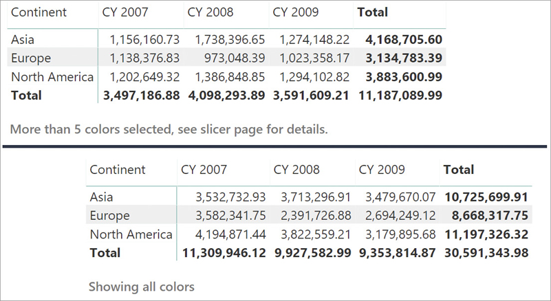
This latter version of the measure is not perfect yet. In the case where the user selects five colors, but only four are present in the current selection because other filters hide some colors, then the measure does not report the complete list of colors. It only reports the existing list. In Chapter 10, “Working with the filter context,” we describe a different version of this measure that addresses this last detail. In fact, to author the final version, we first need to describe a set of new functions that aim at investigating the content of the current filter context.
Iterators returning tables
So far, we have described iterators that aggregate an expression. There are also iterators that return a table produced by merging a source table with one or more expressions evaluated in the row context of the iteration. ADDCOLUMNS and SELECTCOLUMNS are the most interesting and useful. They are the topic of this section.
As its name implies, ADDCOLUMNS adds new columns to the table expression provided as the first parameter. For each added column, ADDCOLUMNS requires knowing the column name and the expression that defines it.
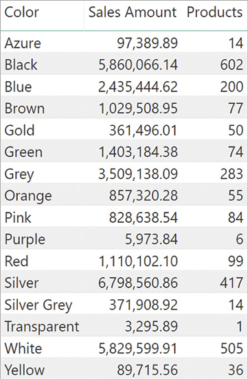
For example, you can add two columns to the list of colors, including for each color the number of products and the value of Sales Amount in two new columns:
Colors =
ADDCOLUMNS (
    VALUES ( 'Product'[Color] ),
    "Products", CALCULATE ( COUNTROWS ( 'Product' ) ),
    "Sales Amount", [Sales Amount]
)
The result of this code is a table with three columns: the product color, which is coming from the values of Product[Color], and the two new columns added by ADDCOLUMNS as you can see in Figure 7-6.
ADDCOLUMNS returns all the columns of the table expression it iterates, adding the requested columns. To keep only a subset of the columns of the original table expression, an option is to use SELECTCOLUMNS, which only returns the requested columns. For instance, you can rewrite the previous example of ADDCOLUMNS by using the following query:
Colors =
SELECTCOLUMNS (
    VALUES ( 'Product'[Color] ),
    "Color", 'Product'[Color],
    "Products", CALCULATE ( COUNTROWS ( 'Product' ) ),
    "Sales Amount", [Sales Amount]
)
The result is the same, but you need to explicitly include the Color column of the original table to obtain the same result. SELECTCOLUMNS is useful whenever you need to reduce the number of columns of a table, oftentimes resulting from some partial calculations.
ADDCOLUMNS and SELECTCOLUMNS are useful to create new tables, as you have seen in this first example. These functions are also often used when authoring measures to make the code easier and faster. As an example, look at the measure, defined earlier in this chapter, that aims at finding the date with the maximum daily sales:
Max Daily Sales :=
MAXX (
    'Date',
    [Sales Amount]
)

Date of Max :=
VAR MaxDailySales = [Max Daily Sales]
VAR DatesWithMax =
    FILTER (
        VALUES ( 'Date'[Date] ),
        [Sales Amount] = MaxDailySales
    )
VAR Result =
    IF (
        COUNTROWS ( DatesWithMax ) = 1,
        DatesWithMax,
        BLANK ()
    )
RETURN
    Result
If you look carefully at the code, you will notice that it is not optimal in terms of performance. In fact, as part of the calculation of the variable MaxDailySales, the engine needs to compute the daily sales to find the maximum value. Then, as part of the second variable evaluation, it needs to compute the daily sales again to find the dates when the maximum sales happened. Thus, the engine performs two iterations on the Date table, and each time it computes the sales amount for each date. The DAX optimizer might be smart enough to understand that it can compute the daily sales only once, and then use the previous result the second time you need it, but this is not guaranteed to happen. Nevertheless, by refactoring the code leveraging ADDCOLUMNS, one can write a faster version of the same measure. This is achieved by first preparing a table with the daily sales and storing it into a variable, then using this first—partial—result to compute both the maximum daily sales and the date with the maximum sales:
Date of Max :=
VAR DailySales =
    ADDCOLUMNS (
        VALUES ( 'Date'[Date] ),
        "Daily Sales", [Sales Amount]
    )
VAR MaxDailySales = MAXX ( DailySales, [Daily Sales] )
VAR DatesWithMax =
    SELECTCOLUMNS (
        FILTER (
            DailySales,
            [Daily Sales] = MaxDailySales
        ),
        "Date", 'Date'[Date]
    )
VAR Result =
IF (
    COUNTROWS ( DatesWithMax ) = 1,
    DatesWithMax,
    BLANK ()
)
RETURN
    Result
The algorithm is close to the previous one, with some noticeable differences:
The DailySales variable contains a table with date, and sales amount on each given date. This table is created by using ADDCOLUMNS.
MaxDailySales no longer computes the daily sales. It scans the precomputed DailySales variable, resulting in faster execution time.
The same happens with DatesWithMax, which scans the DailySales variable. Because after that point the code only needs the date and no longer the daily sales, we used SELECTCOLUMNS to remove the daily sales from the result.
This latter version of the code is more complex than the original version. This is often the price to pay when optimizing code: Worrying about performance means having to write more complex code.
You will see ADDCOLUMNS and SELECTCOLUMNS in more detail in Chapter 12, “Working with tables,” and in Chapter 13, “Authoring queries.” There are many details that are important there, especially if you want to use the result of SELECTCOLUMNS in other iterators that perform context transition.
Solving common scenarios with iterators
In this section we continue to show examples of known iterators and we also introduce a common and useful one: RANKX. You start learning how to compute moving averages and the difference between using an iterator or a straight calculation for the average. Later in this section, we provide a complete description of the RANKX function, which is extremely useful to compute ranking based on expressions.
Computing averages and moving averages
You can calculate the mean (arithmetic average) of a set of values by using one of the following DAX functions:
AVERAGE: returns the average of all the numbers in a numeric column.
AVERAGEX: calculates the average on an expression evaluated over a table.
![]() Note
Note
DAX also provides the AVERAGEA function, which returns the average of all the numbers in a text column. However, you should not use it. AVERAGEA only exists in DAX for Excel compatibility. The main issue of AVERAGEA is that when you use a text column as an argument, it does not try to convert each text row to a number as Excel does. Instead, if you pass a string column as an argument, you always obtain 0 as a result. That is quite useless. On the other hand, AVERAGE would return an error, clearly indicating that it cannot average strings.
We discussed how to compute regular averages over a table earlier in this chapter. Here we want to show a more advanced usage, that is a moving average. For example, imagine that you want to analyze the daily sales of Contoso. If you just build a report that plots the sales amount sliced by day, the result is hard to analyze. As you can see in Figure 7-7, the value obtained has strong daily variations.
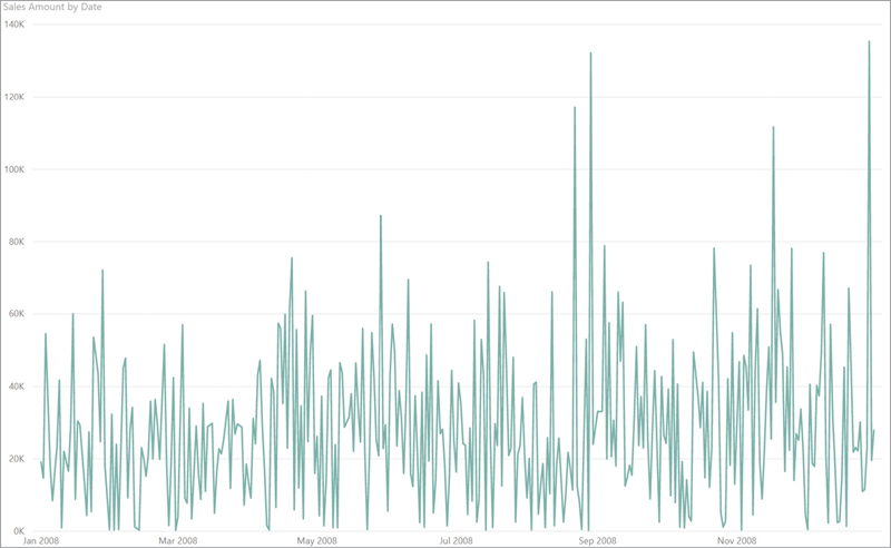
To smooth out the chart, a common technique is to compute the average over a certain period greater than just the day level. In our example, we decided to use 30 days as our period. Thus, on each day the chart shows the average over the last 30 days. This technique helps in removing peaks from the chart, making it easier to detect a trend.
The following calculation provides the average at the date cardinality, over the last 30 days:
AvgXSales30 :=
VAR LastVisibleDate = MAX ( 'Date'[Date] )
VAR NumberOfDays = 30
VAR PeriodToUse =
FILTER (
ALL ( 'Date' ),
AND (
'Date'[Date] > LastVisibleDate - NumberOfDays,
'Date'[Date] <= LastVisibleDate
)
)
VAR Result =
CALCULATE (
AVERAGEX ( 'Date', [Sales Amount] ) ,
PeriodToUse
)
RETURN
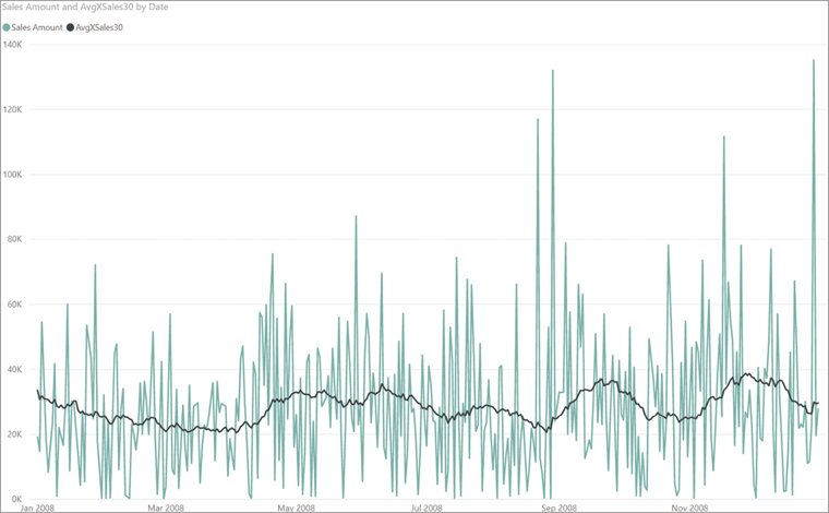
ResultThe formula first determines the last visible date; in the chart, because the filter context set by the visual is at the date level, it returns the selected date. The formula then creates a set of all the dates between the last date and the last date minus 30 days. Finally, the last step is to use this period as a filter in CALCULATE so that the final AVERAGEX iterates over the 30-day period, computing the average of the daily sales.
The result of this calculation is visible in Figure 7-8. As you can see, the line is much smoother than the daily sales, making it possible to analyze trends.
When the user relies on average functions like AVERAGEX, they need to pay special attention to the desired result. In fact, when computing an average, DAX ignores blank values. If on a given day there are no sales, then that day will not be considered as part of the average. Beware that this is a correct behavior. AVERAGEX cannot assume that if there are no sales in a day then we might want to use zero instead. This behavior might not be desirable when averaging over dates.
If the requirement is to compute the average over dates counting days with no sales as zeroes, then the formula to use is almost always a simple division instead of AVERAGEX. A simple division is also faster because the context transition within AVERAGEX requires more memory and increased execution time. Look at the following variation of the moving average, where the only difference from the previous formula is the expression inside CALCULATE:
AvgSales30 :=
VAR LastVisibleDate = MAX ( 'Date'[Date] )
VAR NumberOfDays = 30
VAR PeriodToUse =
    FILTER (
        ALL ( 'Date' ),
        'Date'[Date] > LastVisibleDate - NumberOfDays &&
        'Date'[Date] <= LastVisibleDate
    )
VAR Result =
CALCULATE (
    DIVIDE ( [Sales Amount], COUNTROWS ( 'Date' ) ),
    PeriodToUse
)
RETURN
    Result
Not leveraging AVERAGEX, this latter version of the code considers a day with no sales as a zero. This is reflected in the resulting value whose behavior is similar to the previous one, though slightly different. Moreover, the result of this latter calculation is always a bit smaller than the previous one because the denominator is nearly always a higher value, as you can appreciate in Figure 7-9.
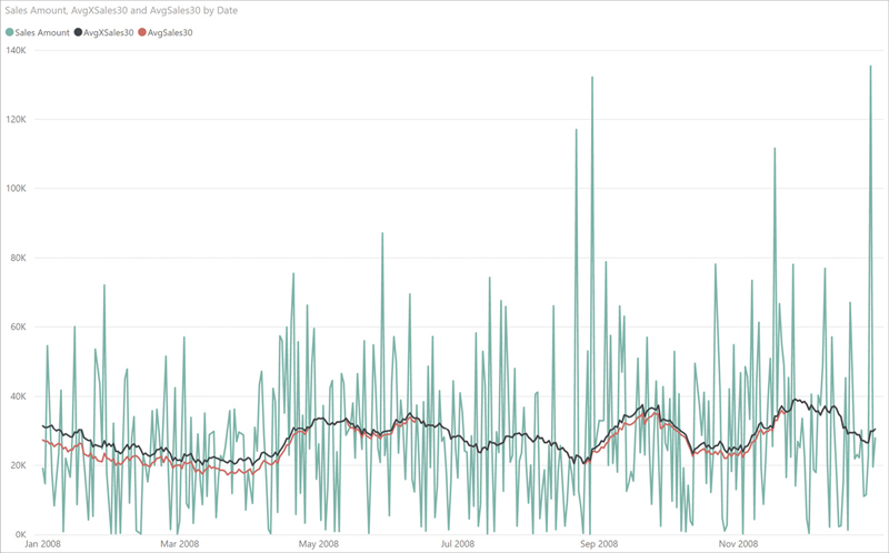
As is often the case with business calculations, it is not that one is better than the other. It all depends on your specific requirements. DAX offers different ways of obtaining the result. It is up to you to choose the right one. For example, by using COUNTROWS the formula now accounts for days with no sales considering them as zeroes, but it also counts holidays and weekends as days with no sales. Whether this is correct or not depends on the specific requirements and the formula needs to be updated in order to reflect the correct average.
Using RANKX
The RANKX function is used to show the ranking value of an element according to a specific sort order. For example, a typical use of RANKX is to provide a ranking of products or customers based on their sales volumes. RANKX accepts several parameters, though most frequently only the first two are used. All the others are optional and seldom used.
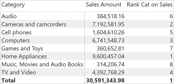
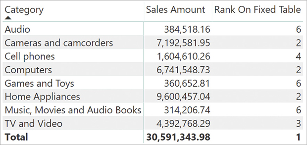
For example, imagine wanting to build the report in Figure 7-10 that shows the ranking of a category against all others based on respective sales amounts.
In this scenario, RANKX is the function to use. RANKX is an iterator and it is a simple function. Nevertheless, its use hides some complexities that are worth a deeper explanation.
The code of Rank Cat on Sales is the following:
Rank Cat on Sales :=
RANKX (
    ALL ( 'Product'[Category] ),
    [Sales Amount]
)
RANKX operates in three steps:
RANKX builds a lookup table by iterating over the table provided as the first parameter. During the iteration it evaluates its second parameter in the row context of the iteration. At the end, it sorts the lookup table.
RANKX evaluates its second parameter in the original evaluation context.
RANKX returns the position of the value computed in the second step by searching its place in the sorted lookup table.
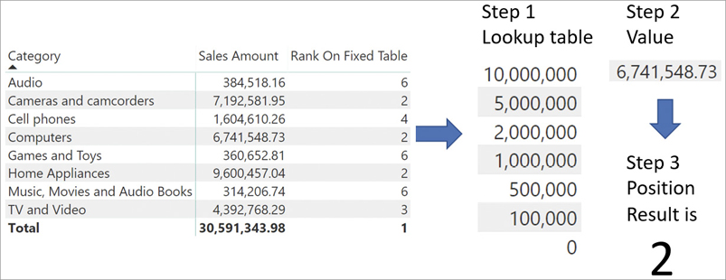
The algorithm is outlined in Figure 7-11, where we show the steps needed to compute the value of 2, the ranking of Cameras and camcorders according to Sales Amount.
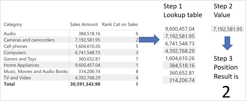
Here is a more detailed description of the behavior of RANKX in our example:
The lookup table is built during the iteration. In the code, we had to use ALL on the product category to ignore the current filter context that would otherwise filter the only category visible, producing a lookup table with only one row.
The value of Sales Amount is a different one for each category because of context transition. Indeed, during the iteration there is a row context. Because the expression to evaluate is a measure that contains a hidden CALCULATE, context transition makes DAX compute the value of Sales Amount only for the given category.
The lookup table only contains values. Any reference to the category is lost: Ranking takes place only on values, once they are sorted correctly.
The value determined in step 2 comes from the evaluation of the Sales Amount measure outside of the iteration, in the original evaluation context. The original filter context is filtering Cameras and camcorders. Therefore, the result is the amount of sales of cameras and camcorders.
The value of 2 is the result of finding the place of Sales Amount of cameras and camcorders in the sorted lookup table.
You might have noticed that at the grand total, RANKX shows 1. This value does not make any sense from a human point of view because a ranking should not have any total at all. Nevertheless, this value is the result of the same process of evaluation, which at the grand total always shows a meaningless value. In Figure 7-12 you can see the evaluation process at the grand total.
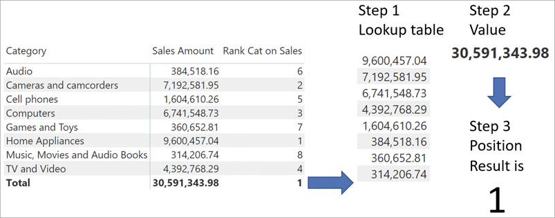
The value computed during step 2 is the grand total of sales, which is always greater than the sum of individual categories. Thus, the value shown at the grand total is not a bug or a defect; it is the standard RANKX behavior that loses its intended meaning at the grand total level. The correct way of handling the total is to hide it by using DAX code. Indeed, the ranking of a category against all other categories has meaning if (and only if) the current filter context only filters one category. Consequently, a better formulation of the measure relies on HASONEVALUE in order to avoid computing the ranking in a filter context that produces a meaningless result:
Rank Cat on Sales :=
IF (
    HASONEVALUE ( 'Product'[Category] ),
    RANKX (
        ALL ( 'Product'[Category] ),
        [Sales Amount]
    )
)
This code produces a blank whenever there are multiple categories in the current filter context, removing the total row. Whenever one uses RANKX or, in more general terms, whenever the measure computed depends on specific characteristics of the filter context, one should protect the measure with a conditional expression that ensures that the calculation only happens when it should, providing a blank or an error message in any other case. This is exactly what the previous measure does.
As we mentioned earlier RANKX accepts many arguments, not only the first two. There are three remaining arguments, which we introduce here. We describe them later in this section.
The third parameter is the value expression, which might be useful when different expressions are being used to evaluate respectively the lookup table and the value to use for the ranking.
The fourth parameter is the sort order of the lookup table. It can be ASC or DESC. The default is DESC, with the highest values on top—that is, higher value results in lower ranking.
The fifth parameter defines how to compute values in case of ties. It can be DENSE or SKIP. If it is DENSE, then ties are removed from the lookup table; otherwise they are kept.
Let us describe the remaining parameters with some examples.
The third parameter is useful whenever one needs to use a different expression respectively to build the lookup table and to compute the value to rank. For example, consider the requirement of a custom table for the ranking, like the one depicted in Figure 7-13.
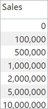
If one wants to use this table to compute the lookup table, then the expression used to build it should be different from the Sales Amount measure. In such a case, the third parameter becomes useful. To rank the sales amount against this specific lookup table—which is named Sales Ranking—the code is the following:
Rank On Fixed Table :=
RANKX (
    'Sales Ranking',
    'Sales Ranking'[Sales],
    [Sales Amount]
)
In this case, the lookup table is built by getting the value of {'Sales Ranking{'[Sale] in the row context of Sales Ranking. Once the lookup table is built, RANKX evaluates [Sales Amount] in the original evaluation context.
The result of this calculation is visible in Figure 7-14.
The full process is depicted in Figure 7-15, where you can also appreciate that the lookup table is sorted before being used.
The fourth parameter can be ASC or DESC. It changes the sort order of the lookup table. By default it is DESC, meaning that a lower ranking is assigned to the highest value. If one uses ASC, then the lower value will be assigned the lower ranking because the lookup table is sorted the opposite way.
The fifth parameter, on the other hand, is useful in the presence of ties. To introduce ties in the calculation, we use a different measure—Rounded Sales. Rounded Sales rounds values to the nearest multiple of one million, and we will slice it by brand:
Rounded Sales := MROUND ( [Sales Amount], 1000000 )
Then, we define two different rankings: One uses the default ranking (which is SKIP), whereas the other one uses DENSE for the ranking:
Rank On Rounded Sales :=
RANKX (
    ALL ( 'Product'[Brand] ),
    [Rounded Sales]
)

Rank On Rounded Sales Dense :=
RANKX (
    ALL ( 'Product'[Brand] ),
    [Rounded Sales],
    ,
    ,
    DENSE
)
The result of the two measures is different. In fact, the default behavior considers the number of ties and it increases the ranking accordingly. When using DENSE, the ranking increases by one regardless of ties. You can appreciate the different result in Figure 7-16.

Basically, DENSE performs a DISTINCT on the lookup table before using it. SKIP does not, and it uses the lookup table as it is generated during the iteration.
When using RANKX, it is important to consider which table to use as the first parameter to obtain the desired result. In the previous queries, it was necessary to specify ALL ( Product[Brand] ) because we wanted to obtain the ranking of each brand. For brevity, we omitted the usual test with HASONEVALUE. In practice you should never skip it; otherwise the measure is at risk of computing unexpected results. For example, a measure like the following one produces an error if not used in a report that slices by Brand:
Rank On Sales :=
RANKX (
    ALL ( 'Product'[Brand] ),
    [Sales Amount]
)
In Figure 7-17 we slice the measure by product color and the result is always 1.

The reason is that the lookup table contains the sales amount sliced by brand and by color, whereas the values to search in the lookup table contain the total only by color. As such, the total by color will always be larger than any of its subsets by brand, resulting in a ranking of 1. Adding the protection code with IF HASONEVALUE ensures that—if the evaluation context does not filter a single brand—the result will be blank.
Finally, ALLSELECTED is oftentimes used with RANKX. If a user performs a selection of some brands out of the entire set of brands, ranking over ALL might produce gaps in the ranking. This is because ALL returns all the brands, regardless of the filter coming from the slicer. For example, consider the following measures:
Rank On Selected Brands :=
RANKX (
    ALLSELECTED ( 'Product'[Brand] ),
    [Sales Amount]
)

Rank On All Brands :=
RANKX (
    ALL ( 'Product'[Brand] ),
    [Sales Amount]
)
In Figure 7-18, you can see the comparison between the two measures in the presence of a slicer filtering certain brands.

Changing calculation granularity
There are several scenarios where a formula cannot be easily computed at the total level. Instead, the same calculation could be performed at a higher granularity and then aggregated later.
Imagine needing to compute the sales amount per working day. The number of working days in every month is different because of the number of Saturdays and Sundays or because of the holidays in a month. For the sake of simplicity, in this example we only consider Saturdays and Sundays, but our readers can easily extend the concept to also considering holidays.
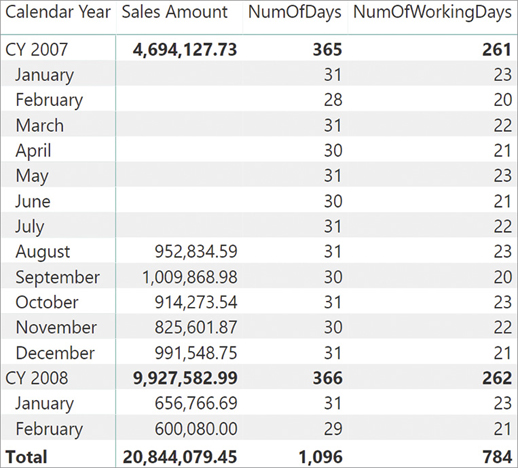
The Date table contains an IsWorkingDay column that contains 1 or 0 depending on whether that day is a working day or not. It is useful to store the information as an integer because it makes the calculation of days and working days very simple. Indeed, the two following measures compute the number of days in the current filter context and the corresponding number of working days:
NumOfDays := COUNTROWS ( 'Date' )
NumOfWorkingDays := SUM ( 'Date'[IsWorkingDay] )
In Figure 7-19 you can see a report with the two measures.
Based on these measures, we might want to compute the sales per working day. That is a simple division of the sales amount by the number of working days. This calculation is useful to produce a performance indicator for each month, considering both the gross amount of sales and the number of days in which sales were possible. Though the calculation looks simple, it hides some complexity that we solve by leveraging iterators. As we sometimes do in this book, we show this solution step-by-step, highlighting possible errors in the writing process. The goal of this demo is not to show a pattern. Instead, it is a showcase of different mistakes that a developer might make when authoring a DAX expression.
As anticipated, a simple division of Sales Amount by the number of working days produces correct results only at the month level. At the grand total, the result is surprisingly lower than any other month:
SalesPerWorkingDay := DIVIDE ( [Sales Amount], [NumOfWorkingDays] )
In Figure 7-20 you can look at the result.
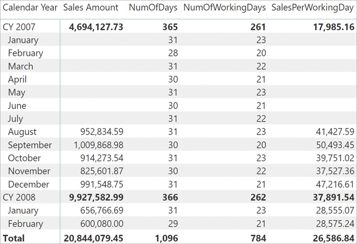
If you focus your attention to the total of 2007, it shows 17,985.16. It is surprisingly low considering that all monthly values are above 37,000.00. The reason is that the number of working days at the year level is 261, including the months where there are no sales at all. In this model, sales started in August 2007 so it would be wrong to consider previous months where there cannot be other sales. The same issue also happens in the period containing the last day with data. For example, the total of the working days in the current year will likely consider future months as working days.
There are multiple ways of fixing the formula. We choose a simple one: if there are no sales in a month, then the formula should not consider the days in that month. This formula assumes that all the months between the oldest transaction and the last transaction available have transactions associated.
Because the calculation must work on a month-by-month basis, it needs to iterate over months and check if there are sales in each month. If there are sales, then it adds the number of working days. If there are no sales in the given month, then it skips it. SUMX can implement this algorithm:
SalesPerWorkingDay :=
VAR WorkingDays =
    SUMX (
        VALUES ( 'Date'[Month] ),
        IF (
            [Sales Amount] > 0,
            [NumOfWorkingDays]
        )
    )
VAR Result =
    DIVIDE (
        [Sales Amount],
        WorkingDays
    )
RETURN
    Result
This new version of the code provides an accurate result at the year level, as shown in Figure 7-21, though it is still not perfect.
When performing the calculation at a different granularity, one needs to ensure the correct level of granularity. The iteration started by SUMX iterates the values of the month column, which are January through December. At the year level everything is working correctly, but the value is still incorrect at the grand total. You can observe this behavior in Figure 7-22.

When the filter context contains the year, an iteration of months works fine because—after the context transition—the new filter context contains both a year and a month. However, at the grand total level, the year is no longer part of the filter context. Consequently, the filter context only contains the currently iterated month, and the formula does not check if there are sales in that year and month. Instead, it checks if there are sales in that month for any year.
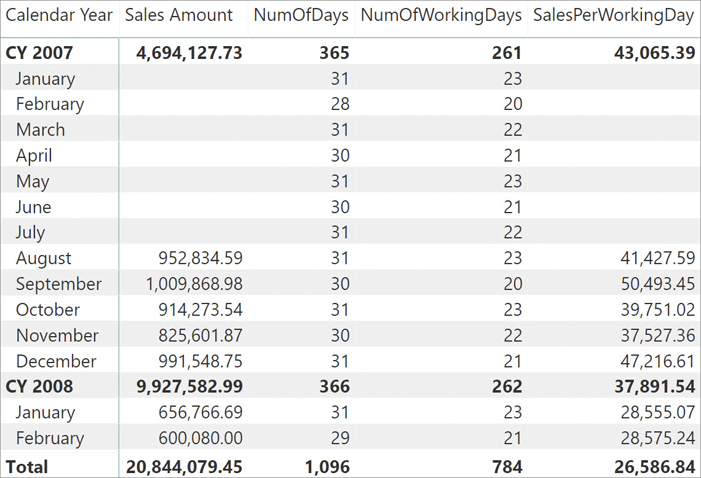
The problem of this formula is the iteration over the month column. The correct granularity of the iteration is not the month; it is the pair of year and month together. The best solution is to iterate over a column containing a different value for each year and month. It turns out that we have such a column in the data model: the Calendar Year Month column. To fix the code, it is enough to iterate over the Calendar Year Month column instead of over Month:
SalesPerWorkingDay :=
VAR WorkingDays =
    SUMX (
        VALUES ( 'Date'[Calendar Year Month] ),
        IF (
            [Sales Amount] > 0,
            [NumOfWorkingDays]
        )
    )
VAR Result =
    DIVIDE (
        [Sales Amount],
        WorkingDays
    )
RETURN
    Result
This final version of the code works fine because it computes the total using an iteration at the correct level of granularity. You can see the result in Figure 7-23.

Conclusions
As usual, let us conclude this chapter with a recap of the important concepts you learned here:
Iterators are an important part of DAX, and you will find yourself using them more, the more you use DAX.
There are mainly two kinds of iterations in DAX: iterations to perform simple calculations on a row-by-row basis and iterations that leverage context transition. The definition of Sales Amount we used so far in the book uses an iteration to compute the quantity multiplied by the net price, on a row-by-row basis. In this chapter, we introduced iterators with a context transition, a powerful tool to compute more complex expressions.
Whenever using an iterator with context transition, you must check the cardinality the iteration should happen at—it should be quite small. You also need to check that the rows in the table are guaranteed to be unique. Otherwise, the code is at risk of being slow or of computing bad results.
When computing averages over time, you always should check whether an iterator is the correct solution or not. AVERAGEX does not consider blanks as part of its calculation and, when using time, this could be wrong. Nevertheless, always double-check the formula requirements; each scenario is unique.
Iterators are useful to compute values at a different granularity, as you learned in the last example. When dealing with calculations at different granularities, it is of paramount importance to check the correct granularity to avoid errors in the code.
You will see many more examples of iterators in the remaining part of the book. Starting from the next chapter, when dealing with time intelligence calculations, you will see different calculations, most of which rely on iterations.