Chapter 3
Design and implement an on-premises database infrastructure
This chapter covers the architecture of an on-premises database infrastructure, including the differences between data and transaction log files, and how certain features work to ensure durability and consistency even during unexpected events.
We cover what certain important configuration settings mean, both from a performance and best-practice perspective. We also go into detail about the different kinds of data compression and file system settings that are most appropriate for your environment.
The sample scripts in this chapter, and all scripts for this book, are available for download at https://www.MicrosoftPressStore.com/SQLServer2022InsideOut/downloads.
Introduction to SQL Server database architecture
The easiest way to observe the implementation of a SQL Server database is by its files. Every SQL Server database has at least two main kinds of files:
Data. The data itself is stored in one or more filegroups. Each filegroup in turn comprises one or more physical data files.
Transaction log. This is where all data modifications are saved until committed or rolled back and then hardened to a data file. There is usually only one transaction log file per database.
Note
There are several other file types used by SQL Server, including logs, trace files, and memory-optimized filegroups, which we discuss later in this chapter.
Data files and filegroups
When you create a user database without specifying any overriding settings, SQL Server uses the model database as a template. This provides your new database with its default configuration, including ownership, compatibility level, file growth settings, recovery model (full, bulk-logged, simple), and physical file settings.
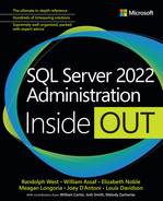
By default, each new database has one transaction log file and one data filegroup. This data filegroup is known as the primary filegroup, comprising a single data file by default. It is known as the primary data file, which has the file extension .mdf. (See Figure 3-1.)
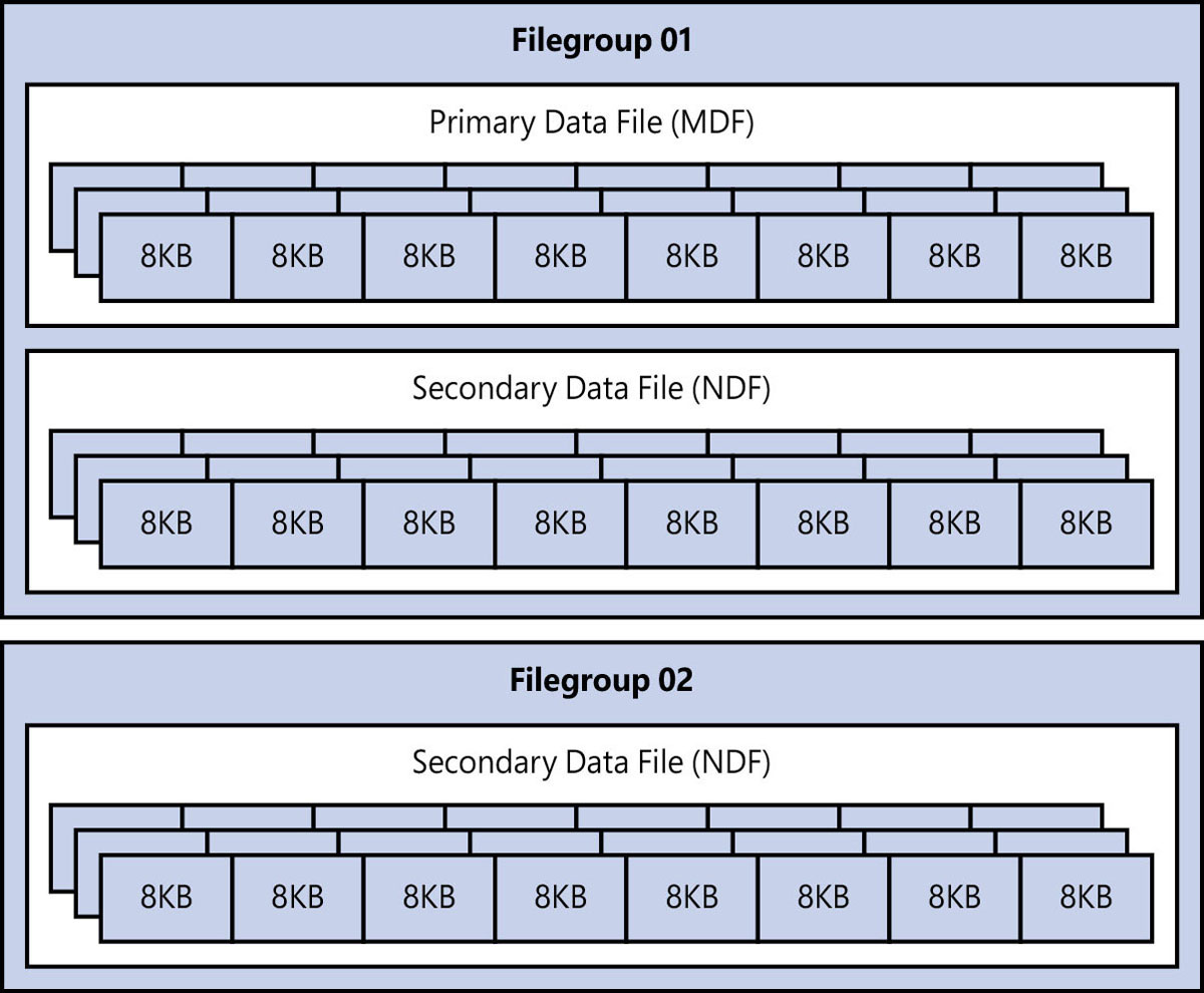
Figure 3-1 The data files as they make up one or more filegroups in a database.
Note
The file extensions used for SQL Server data and transaction log files are listed by convention only and are not required.
You can have more than one file in a filegroup, which can provide better performance through parallel reads and writes (but please test this scenario before adding too many files). Secondary data files generally have the file extension .ndf.
For large databases (more than 100 GB), you can separate your data into multiple filegroups based on a business rule (one per year, for instance). The real benefit comes with adding new filegroups and splitting your logical data storage across those filegroups. This makes it possible for you to do things like piecemeal backups and online restores at a filegroup level in Enterprise edition. Only offline filegroup restore is available in Standard edition.
You can also age-out data into a filegroup that is set to read-only and store it on slower storage than the current data, to manage storage costs better.
If you use table partitioning (see the “Partition tables” section later in the chapter), splitting partitions across filegroups makes even more sense.
Group data pages with extents
SQL Server data pages are 8 KB in size. Eight of these contiguous pages is called an extent, which is 64 KB in size.
There are two types of extents in a SQL Server data file:
Uniform extent. All eight 8-KB pages per extent are assigned to a single object.
Mixed extent (rare). Each page in the extent is assigned to its own separate object (one 8-KB page per object).
Mixed extents were originally created to reduce storage requirements for database objects, back when mechanical hard drives were much smaller and more expensive. As storage becomes faster and cheaper, and SQL Server more complex, contention (a hotspot) can occur at the beginning of a data file, especially if a lot of small objects are being created and deleted.
Mixed extents are turned off by default for tempdb and user databases, and are turned on by default for system databases. If you want, you can configure mixed extents on a user database by using the following command:
ALTER DATABASE <dbname> SET MIXED_PAGE_ALLOCATION ON;Contents and types of data pages
All data pages begin with a header of 96 bytes, followed by a body containing the data itself. At the end of the page is a slot array, which fills up in reverse order, beginning with the first row, as illustrated in Figure 3-2. It instructs the Database Engine where a particular row begins on that particular page. Note that the slot array does not need to be in any particular order after the first row.

Figure 3-2 A typical 8-KB data page, showing the header, the data, and the slot array.
At certain points in the data file, there are system-specific data pages (also 8 KB in size). These help SQL Server recognize and manage the different data within each file.
Several types of pages can be found in a data file:
Data. Regular data from a heap or a clustered index at the leaf level (the data itself; what you would see when querying a table).
Index. Non-clustered index data at the leaf and non-leaf level, as well as clustered indexes at the non-leaf level.
Text/image. Sometimes referred to as large object (LOB) data types. These include
text,ntext,image,nvarchar(max),varchar(max),varbinary(max), Common Language Runtime (CLR) data types,xml, andsql_variantwhere it exceeds 8 KB. Overflow data can also be stored here (data that has been moved off-page by the Database Engine), with a pointer from the original page.Global Allocation Map (GAM). Keeps track of all free extents in a data file. There is one GAM page for every GAM interval (64,000 extents, or roughly 4 GB).
Shared Global Allocation Map (SGAM). Keeps track of all extents that can be mixed extents. It has the same interval as the GAM.
Page Free Space (PFS). Keeps track of free space inside heap and large object pages. There is one PFS page for every PFS interval (8,088 pages, or roughly 64 MB).
Index Allocation Map (IAM). Keeps track of which extents in a GAM interval belong to a particular allocation unit. (An allocation unit is a bucket of pages that belong to a partition, which in turn belongs to a table.) It has the same interval as the GAM. There is at least one IAM for every allocation unit. If more than one IAM belongs to an allocation unit, it forms an IAM chain.
Bulk Changed Map (BCM). Keeps track of extents modified by bulk-logged operations since the last full backup. It is used by transaction log backups in the bulk-logged recovery model to see which extents should be backed up.
Differential Changed Map (DCM). Sometimes called a differential bitmap. Keeps track of extents that were modified since the last full or differential backup. Used for differential backups.
Boot page. Contains information about the database. There is only one boot page per database.
File header page. Contains information about the file. There is only one per data file.
 To find out more about the internals of a data page, visit https://learn.microsoft.com/sql/relational-databases/pages-and-extents-architecture-guide and read Paul Randal’s post, “Inside the Storage Engine: Anatomy of a page,” at https://www.sqlskills.com/blogs/paul/inside-the-storage-engine-anatomy-of-a-page.
Verify data pages by using a checksum
By default, when a data page is read into the buffer pool, a checksum is automatically calculated over the entire 8-KB page and compared to the checksum stored in the page header on the drive. This is how SQL Server keeps track of page-level corruption—by detecting when the contents of a data page do not match the results the Database Engine expects. This corruption can happen through storage failures, physical memory corruption, or SQL Server bugs. If the checksum stored on the drive does not match the checksum in memory, corruption has occurred. A record of this suspect page is stored in the msdb database, and you will see an error message when that page is accessed.
The same checksum is performed when writing to a drive. If the checksum on the drive does not match the checksum in the data page in the buffer pool, page-level corruption has occurred.
Although the PAGE_VERIFY property on new databases is set to CHECKSUM by default, it might be necessary to check databases that have been upgraded from previous versions of SQL Server, especially those created prior to SQL Server 2005 (compatibility level 90).
You can look at the checksum verification status on all databases by using the following query:
SELECT name, page_verify_option_desc
FROM sys.databases;
You can reduce the likelihood of data page corruption by using error-correcting code (ECC) memory. Data page corruption on the drive is detected by using DBCC CHECKDB and other operations.
- For information on how to proactively detect corruption, review the sections on database corruption in Chapter 8, “Maintain and monitor SQL Server.”
Record changes in the transaction log
The transaction log is the most important component of a SQL Server database because it is where all units of work (transactions) performed on a database are recorded, before the data can be written (flushed) to the drive. The transaction log file usually has the file extension .ldf.
Note
Although it is possible to use more than one file to store the transaction logs for a database, we do not recommend this because there is no performance or maintenance benefit to using multiple files. To understand why and where it might be appropriate to have more than one, see the section “Inside the transaction log file” later in the chapter.
A successful transaction is said to be committed. An unsuccessful and completely reversed transaction is said to be rolled back.
In Chapter 2, we saw that when SQL Server needs an 8-KB data page from the data file, it usually (if the page doesn’t already exist in the buffer pool) copies it from the drive and stores a copy of it in memory in an area called the buffer pool while that page is required. When a transaction needs to modify that page, it works directly on the copy of the page in the buffer pool. If the page is subsequently modified, a log record of the modification is created in the log buffer (also in memory), and that log record is then written to the drive. This process happens synchronously—a transaction is not considered complete by the Database Engine until it is written into the transaction log.
SQL Server uses a technique called write-ahead logging (WAL), which ensures that no changes are written to the data file before the necessary log record is written to the drive in a permanent form (in this case, non-volatile storage).
However, you can use delayed durability (also known as lazy commit), which does not save every change to the transaction log as it happens. Instead, it waits until the log cache grows to a certain size (or sp_flushlog runs) before flushing it to the drive.
Caution
If you turn on delayed durability for your database, the performance benefit has a downside of potential data loss if the underlying storage layer experiences a failure before the log can be saved. Indeed, sp_flushlog should also be run before shutting down SQL Server for all databases with delayed durability enabled.
- You can read more about log persistence and how it affects durability of transactions in Chapter 14, “Performance tune SQL Server,” and at https://learn.microsoft.com/sql/relational-databases/logs/control-transaction-durability.
A transaction’s outcome is unknown until a commit or rollback occurs. An error might occur during a transaction, or the operator might decide to roll back the transaction manually because the results were not as expected. In the case of a rollback, changes to the modified data pages must be undone. SQL Server will use the saved log records to undo the changes for an incomplete transaction.
Only when the transaction log file is written to can the modified 8-KB page be saved in the data file, though the page might be modified several times in the buffer pool before it is flushed to the drive using a checkpoint operation.
Our guidance, therefore, is to use the fastest storage possible for the transaction log file(s), because of the low-latency requirements.
Flush data to the storage subsystem with checkpoints
Recall from Chapter 2 that any changes to data are written to the database file asynchronously for performance reasons. This process is controlled by a database checkpoint. As its name implies, this is a database-level setting that can be changed under certain conditions by modifying the recovery interval or running the CHECKPOINT command in the database context.
The checkpoint process takes all the modified pages in the buffer pool, as well as transaction log information that is in memory, and writes it to the storage subsystem. This reduces the time it takes to recover a database because only the changes made after the latest checkpoint need to be rolled forward in the Redo phase (see the “Restart with recovery” section later in the chapter).
Inside the transaction log file
A transaction log file is split into logical segments, called virtual log files (VLFs). These segments are dynamically allocated when the transaction log file is created and whenever the file grows. The size of each VLF is not fixed, and is based on an internal algorithm, which depends on the version of SQL Server, the current file size, and file growth settings. Each VLF has a header containing a minimum log sequence number and information indicating whether the VLF is active.
Every transaction is uniquely identified by a log sequence number (LSN). Each LSN is ordered, so a later LSN will be greater than an earlier LSN. The LSN is also used by database backups and restores.
- For more information see Chapter 8, and Chapter 10, “Develop, deploy, and manage data recovery.”
Figure 3-3 illustrates how the transaction log is circular. When a VLF is first allocated by creation or file growth, it is marked inactive in the VLF header. Transactions can be recorded only in active portions of the log file, so the Database Engine looks for inactive VLFs sequentially. Then, as it needs them, the Database Engine marks them as active to allow transactions to be recorded.
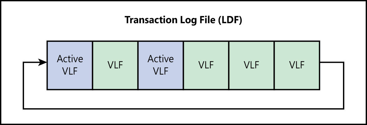
Figure 3-3 The transaction log file, showing active and inactive VLFs.
The operation to make a VLF inactive is called log truncation, but this operation does not affect the size of the physical transaction log file. It just means that an active VLF has been marked inactive and can be reused.
There are several reasons why log truncation can be delayed. After the transactions that use an active VLF are committed or rolled back, what happens next depends on several factors:
The recovery model
Simple. An automatic checkpoint is queued after the recovery interval timeout is reached or if the log becomes 70 percent full.
Full or bulk-logged. A transaction log backup must take place after a transaction is committed. A checkpoint is queued if the log backup is successful.
Other processes that can delay log truncation:
Active backup or restore. The transaction log cannot be truncated if it is being used by a backup or restore operation.
Active transaction. If another transaction is using an active VLF, it cannot be truncated.
Availability group replica. Availability group changes must be synchronized before the log can be truncated. This occurs in high-performance mode or if the mirror is behind the principal database.
Replication. Transactions that have not yet been delivered to the distribution database can delay log truncation.
Oldest page. If a database is configured to use indirect checkpoints, the oldest page in the database might be older than the log sequence number (LSN), which can delay truncation.
Database snapshot creation. This is usually brief, but creating snapshots (manually or through database consistency checks, for instance) can delay truncation.
Log scan. Usually brief, but this, too, can delay a log truncation.
Checkpoint operation. See the section “Flush data to the storage subsystem with checkpoints” earlier in the chapter.
In-Memory OLTP checkpoint. A checkpoint for In-Memory OLTP needs to be performed for memory-optimized tables. An automatic checkpoint is created when the transaction log is larger than 1.5 GB since the last checkpoint.
- To learn more, read “Factors that can delay log truncation” at https://learn.microsoft.com/sql/relational-databases/logs/the-transaction-log-sql-server#FactorsThatDelayTruncation.
After the checkpoint is issued and the dependencies on the transaction log (as just listed) are removed, the log is truncated by marking those VLFs as inactive.
The log is accessed sequentially in this manner until it gets to the end of the file. At this point, the log wraps around to the beginning, and the Database Engine looks for an inactive VLF from the start of the file to mark active. If there are no inactive VLFs available, the log file must create new VLFs by growing according to the auto growth settings.
If the log file cannot grow, it will stop all operations on the database until VLFs can be reclaimed or created.
The Minimum Recovery LSN
When a checkpoint occurs, a log record is written to the transaction log stating that a checkpoint has commenced. After this, the Minimum Recovery LSN (MinLSN) must be recorded. The MinLSN is the minimum of either the LSN at the start of the checkpoint, the LSN of the oldest active transaction, or the LSN of the oldest replication transaction that hasn’t been delivered to the transactional replication distribution database. In other words, the MinLSN “…is the log sequence number of the oldest log record that is required for a successful database-wide rollback” (https://learn.microsoft.com/sql/relational-databases/sql-server-transaction-log-architecture-and-management-guide).
- To learn more about the distribution database, read about replication in Chapter 11, “Implement high availability and disaster recovery.”
This way, crash recovery knows to start recovery only at the MinLSN and can skip over any older LSNs in the transaction log (if they exist). This process minimizes the number of records to be processed at database startup, after a restore.
The checkpoint also records the list of active transactions that have made changes to the database. If the database is in the simple recovery model, the unused portion of the transaction log before the MinLSN is marked for reuse. All dirty data pages and information about the transaction log are written to the storage subsystem, the end of the checkpoint is recorded in the log, and (importantly) the LSN from the start of the checkpoint is written to the boot page of the database.
Note
In the full and bulk-logged recovery models, a successful transaction log backup issues a checkpoint implicitly.
Types of database checkpoints
Checkpoints can be activated in a number of different scenarios. The most common is the automatic checkpoint, which is governed by the recovery interval setting (see the Inside OUT sidebar that follows to see how to modify this setting) and by default takes place approximately once every minute for active databases (those databases in which a change has occurred at all).
Note
Infrequently accessed databases with no transactions do not require a frequent checkpoint, because nothing has changed in the buffer pool.
Other checkpoint events include the following:
Database backups (including transaction log backups)
Database shutdowns
Adding or removing files on a database
SQL Server instance shutdown
Minimally logged operations (for example, in a database in the simple or bulk-logged recovery model)
Explicit use of the
CHECKPOINTcommand
Four types of checkpoints can occur:
Automatic. Issued internally by the Database Engine to meet the value of the recovery interval setting at the instance level. On SQL Server 2016 and higher, the default is 1 minute.
Indirect. Issued to meet a user-specified target recovery time at the database level if the
TARGET_RECOVERY_TIMEhas been set.Manual. Issued when the
CHECKPOINTcommand is run.Internal. Issued internally by various operations, such as backup and snapshot creation, to ensure consistency between the log and the drive image.
- For more information about checkpoints, visit https://learn.microsoft.com/sql/relational-databases/logs/database-checkpoints-sql-server.
Restart with recovery
Whenever SQL Server starts, recovery (also referred to as crash recovery or restart recovery) takes place on every single database (on at least one thread per database, to ensure that it completes as quickly as possible) because SQL Server does not know for certain whether each database was shut down cleanly.
The transaction log is read from the latest checkpoint in the active portion of the log, or the LSN it gets from the boot page of the database (see the “The Minimum Recovery LSN” section earlier in the chapter), and scans all active VLFs looking for work to do.
All committed transactions are rolled forward (Redo portion) and then all uncommitted transactions are rolled back (Undo portion). This process ensures that the data that was written to the transaction log, but did not yet make it into the data files, is played back into the data files. The total number of rolled forward and rolled back transactions are recorded for each database with a respective entry in the SQL Server Error Log file.
SQL Server Enterprise edition brings the database online immediately after the Redo portion is complete. Other editions must wait for the Undo portion to complete before the database is brought online.
- See Chapter 8 for more information about database corruption and recovery.
The reason we cover this in such depth in this introductory chapter is to help you to understand why drive performance is paramount when creating and allocating database files.
When a transaction log file is created or file growth occurs, the portion of the drive must be stamped with a known starting value. (The file system literally writes the binary value 0xC0 in every byte in that file segment.) This is commonly called zeroing out because the binary value was 0x00 prior to SQL Server 2016.
As you can imagine, this can be time consuming for larger files, so you need to take care when setting file growth options—especially with transaction log files. You should measure the performance of the underlying storage layer and choose a fixed growth size that balances performance with reduced VLF count. Instant file initialization does not apply to the initial allocation of transaction log files during restore or recovery. A large transaction log file could impact the duration.
MinLSN and the active log
As mentioned, each VLF contains a header that includes an LSN and an indicator as to whether that VLF is active. The portion of the transaction log from the VLF containing the MinLSN to the VLF containing the latest log record is considered the active.
All records in the active log are required to perform a full recovery if something goes wrong. The active log must therefore include all log records for uncommitted transactions, too, which is why long-running transactions can be problematic. Replicated transactions that have not yet been delivered to the distribution database can also affect the MinLSN.
Any type of transaction that does not allow the MinLSN to increase during the normal course of events affects the overall health and performance of the database environment, because the transaction log file might grow uncontrollably.
When VLFs cannot be made inactive until a long-running transaction is committed or rolled back, or if a VLF is in use by other processes (including database mirroring, availability groups, and transactional replication, for example), the log file is forced to grow. Any log backups that include these long-running transaction records will also be large. The recovery phase can therefore take longer because there is a much larger volume of active transactions to process.
- You can read more about transaction log file architecture at https://learn.microsoft.com/sql/relational-databases/sql-server-transaction-log-architecture-and-management-guide.
A faster recovery with accelerated database recovery
SQL Server 2019 introduced accelerated database recovery (ADR), which can be enabled at the database level. If you are using Azure SQL Database, ADR is enabled by default. At a high level, ADR trades extra space in the data file for reduced space in the transaction log, and for improved performance during manual transaction rollbacks and crash recovery—especially in environments where long-running transactions are common.
It is made up of four components:
Persisted version store (PVS). This works in a similar way to read committed snapshot isolation (RCSI), recording a previously committed version of a row until a transaction is committed. The main difference is that the PVS is stored in the user database and not in tempdb, which allows database-specific changes to be recorded in isolation from other instance-level operations.
Logical revert. If a long-running transaction is aborted, the versioned rows created by the PVS can be safely ignored by concurrent transactions. Additionally, upon rollback, the previous version of the row is immediately made available by releasing all locks.
Secondary log stream (sLog). The sLog is a low-volume in-memory log stream that records non-versioned operations (including lock acquisitions). It is persisted to the transaction log file during a checkpoint operation and is aggressively truncated when transactions are committed.
Cleaner. This asynchronous process periodically cleans page versions that are no longer required. SQL Server 2022 introduces a multi-threaded version cleanup—beneficial when you have a small number of large databases on a given server. Beyond multi-threading the version cleaner process consumes less memory and capacity.
SQL Server 2022 also introduces user transaction cleanup, which clears pages in the version store that could not be cleaned up due to table-level locks blocking the cleanup the process. Beyond these changes, the ADR process has been better optimized to consume fewer resources.
Where ADR shines is in the Redo and Undo phases of crash recovery. In the first part of the Redo phase, the sLog is processed first. Because it contains only uncommitted transactions since the last checkpoint, it is processed extremely quickly. The second part of the Redo phase begins from the last checkpoint in the transaction log, as opposed to the oldest committed transaction.
In the Undo phase, ADR completes almost instantly by first undoing non-versioned operations recorded by the sLog, and then performing a logical revert on row-level versions in the PVS and releasing all locks.
Customers using this feature may notice faster rollbacks, a significant reduction in transaction log usage for long-running transactions, faster SQL Server startup times, and a small increase in the size of the data file for each database where this is enabled (on account of the storage required for the PVS). As with all features of SQL Server, we recommend that you do testing before enabling this on all production databases.
Partition tables
SQL Server allows you to break up the storage of a table or index into logical units, or partitions, for easier management and maintenance while still treating it as a single table. All tables in SQL Server are already partitioned if you look deep enough into the internals. It just so happens that there is one logical partition per table by default.
- Chapter 7, “Understand table features,” goes into more detail about table partitioning.
This concept is called horizontal partitioning. Suppose a database table is growing extremely large, and adding new rows is time consuming. You might decide to split the table into groups of rows, based on a partitioning key (typically a date column), with each group in its own partition. You can then store these in different filegroups to improve read and write performance.
Breaking up a table into logical partitions can also result in a query optimization called partition elimination, by which only the partition that contains the data you need is queried. However, it was not designed primarily as a performance feature. Partitioning tables will not automatically result in better query performance; in fact, performance might be worse due to other factors, specifically around statistics.
Even so, there are some major advantages to table partitioning, which benefit large datasets, specifically around rolling windows and moving data in and out of the table. This process is called partition switching, by which you can switch data into and out of a table almost instantly.
Assume you need to load data into a table every month and then make it available for querying. With table partitioning, you put the data you want to insert into a separate table in the same database, which has the same structure and clustered index as the main table. Then, a switch operation moves that data into the partitioned table almost instantly because no data movement is needed.
This makes it very easy to manage large groups of data or data that ages out at regular intervals (sliding windows), because partitions can be switched out nearly immediately.
Compress data
SQL Server supports several types of data compression to reduce the amount of drive space required for data and backups, as a trade-off against higher CPU utilization.
- You can read more about data compression https://learn.microsoft.com/sql/relational-databases/data-compression/data-compression.
In general, the amount of CPU overhead required to perform compression and decompression depends on the type of data involved, and in the case of data compression, the type of queries running against the database, as well. Even though the higher CPU load might be offset by the savings in I/O, we always recommend testing before implementing this feature.
Table and index compression
SQL Server includes several options for compressing data stored in tables and indexes. We discuss compressing rowstore data in this section. You can read more about columnstore indexes in Chapter 15, “Understand and design indexes.”
Note
SQL Server 2019 introduced a new collation type, UTF-8, which may improve storage of Latin-based strings. See Chapter 7 for more information.
Row compression
You turn on row compression at the table or index level, or on the individual partition level for partitioned objects. Each column in a row is evaluated according to the type of data and contents of that column, as follows:
Numeric data types (such as integer, decimal, floating point, datetime, money, and their derived types) are stored as variable-length strings at the physical layer.
Fixed-length character data types are stored as variable-length strings, where the blank trailing characters are not stored.
Variable-length data types, including large objects, are not affected by row compression.
Bit columns consume more space due to associated metadata.
Row compression can be useful for tables with fixed-length character data types and where numeric types are overprovisioned (e.g., a bigint column that contains mostly int values). Unicode compression alone can save between 15 and 50 percent, depending on your locale and collation.
- You can read more about row compression at https://learn.microsoft.com/sql/relational-databases/data-compression/row-compression-implementation.
Page compression
You enable page compression at the table or index level, but it operates on all data pages associated with that table, including indexes, table partitions, and index partitions. Leaf-level pages (look ahead to Figure 3-4) are compressed using three steps:
Row compression
Prefix compression
Dictionary compression
Non-leaf-level pages are compressed using row compression only. This is for performance reasons.
Figure 3-4 A small clustered index with leaf and non-leaf levels, clustered on ColID.
- You can read more about indexes in Chapter 7, Chapter 14, and Chapter 15. To learn more about index structures, visit https://learn.microsoft.com/sql/relational-databases/sql-server-index-design-guide.
Prefix compression works per column, by searching for a common prefix in each column—for example, the values AAAB and AAAC. In this case, the values of AAA would be moved to the header. A row is created just below the page header, called the compression information (CI) structure, containing a single row of each column with its own prefix. If any of a single column’s rows on the page match the prefix, its value is replaced by a reference to that column’s prefix.
Dictionary compression then searches across the entire page, looking for repeating values (irrespective of the column), and stores these in the CI structure. When a match is found, the column value in that row is replaced with a reference to the compressed value.
If a data page is not full, it will be compressed using only row compression. If the size of the compressed page along with the size of the CI structure is not significantly smaller than the uncompressed page, no page compression will be performed on that page.
Compress and decompress Transact-SQL functions
While page and row compression act on most data types, they do not work well on binary large object (BLOB) data types, such as videos, images, and text documents. With the ability to store JSON documents in SQL Server 2016, Microsoft introduced the COMPRESS and DECOMPRESS T-SQL functions, which use standard gzip compression to compress the data itself.
In SQL Server 2022, there is a dedicated method for compressing off-row XML data for both columns and indexes. XML compression is defined as part of the CREATE TABLE and CREATE INDEX statements.
Backup compression
Whereas page-level and row-level compression operate at the table and index level, backup compression applies to the backup file for the entire database.
Compressed backups are usually smaller than uncompressed backups. This means fewer I/O operations are involved, which in turn reduces the time it takes to perform a backup or restore. For larger databases, this can have a dramatic effect on how long it takes to recover from a disaster.
The backup compression ratio is affected by the type of data involved, whether the database is encrypted, and whether the data is already compressed. In other words, a database using page and/or row compression might not gain any benefit from backup compression.
The CPU can be limited for backup compression in Resource Governor.
- You can read more about Resource Governor in the section “Configuration settings” later in this chapter, and in more detail in Chapter 8.
In most cases, we recommend turning on backup compression, keeping in mind that you might need to monitor CPU utilization.
Intel QuickAssist Technology
SQL Server 2022 introduces support for Intel QuickAssist Technology (Intel QAT) data compression with SQL Server backups. This can potentially double your backup speed and reduces storage capacity by approximately 5 percent. The Intel QAT backup compression requires that you install Intel QAT drivers on the server.
- You can read more about integrated acceleration and offloading at https://learn.microsoft.com/sql/relational-databases/integrated-acceleration/use-integrated-acceleration-and-offloading.
Manage the temporary database
tempdb is the working area of every database on the instance, and there is only one tempdb per instance. SQL Server uses this temporary database for several things that are mostly invisible to you, including temporary tables, table variables, triggers, cursors, sorting, version data for snapshot isolation and read-committed snapshot isolation, index creation, user-defined functions, and many more.
Additionally, when performing queries with operations that don’t fit in memory (the buffer pool and the buffer pool extension), these operations spill to the drive, requiring the use of tempdb.
Storage options for tempdb
Every time SQL Server restarts, tempdb is cleared out. If tempdb’s data and log files don’t exist, they are re-created. If the files are configured at a size that is different from their last active size, they will automatically be resized as they are re-created at startup. Like the database file structure described earlier, there is usually one tempdb transaction log file and one or more data files in a single filegroup.
Performance is critical for tempdb—even more than with other databases—to the point that the current recommendation is to use your fastest storage for tempdb before using it for user database transaction log files.
Where possible, use solid-state storage for tempdb. If you have a failover cluster instance, have tempdb on local storage on each node.
Starting with SQL Server 2019, tempdb can store certain metadata in memory-optimized tables for increased performance.
SQL Server 2022 introduces performance enhancements to two internal page types: Global Allocation Map (GAM) and Shared Global Allocation Map (SGAM) pages, in both user databases and tempdb. These enhancements benefit tempdb-heavy workloads. Workloads that may benefit include, for example, busy databases with read-committed snapshot isolation or applications that make heavy use of temporary tables.
Recommended number of files
As with every database, only one transaction log file should exist for tempdb.
For physical and virtual servers, the default number of tempdb data files recommended by SQL Server Setup should match the number of logical processor cores, up to a maximum of eight, keeping in mind that your logical core count includes symmetrical multithreading (for example, Hyper-Threading). Adding more tempdb data files than the number of logical processor cores rarely results in improved performance. In fact, adding too many tempdb data files could severely harm SQL Server performance.
- You can read more about processors in Chapter 2.
Increasing the number of files to eight (and possibly more, based on other factors) reduces tempdb contention when allocating temporary objects, as processes seek out allocation pages in the buffer pool. If the instance has more than eight logical processors allocated, you can test to see whether adding more files helps performance. This is very much dependent on the workload.
You can allocate the tempdb data files together on the same volume (see the “Types of storage” section in Chapter 2), provided the underlying storage layer can meet the low-latency demands of tempdb on your instance. If you plan to share the storage with other database files, keep latency and IOPS in mind.
Configuration settings
SQL Server has scores of settings that you can tune to your workload. There are also best practices regarding the appropriate settings (such as file growth, memory settings, and parallelism). We cover some of these in this section.
- Chapter 6, “Provision and configure SQL Server databases,” contains additional configuration settings for provisioning databases.
Manage system usage with Resource Governor
Using Resource Governor, you can specify limits on resource consumption at the application-session level. You can configure these in real time, which allows for flexibility in managing workloads without affecting other workloads on the system.
- You can find out more about Resource Governor in Chapter 8.
A resource pool represents the physical resources of an instance, which means you can think of a resource pool itself as a mini SQL Server instance. This allows a DBA to determine quality of service for various workloads on the server.
To make the best use of Resource Governor, it is helpful to logically group similar workloads together into a workload group so you can manage them under a specific resource pool. For example, suppose a reporting application has a negative impact on database performance due to resource contention at certain times of the day. By classifying it into a specific workload group, you can limit the amount of memory or disk I/O that the reporting application can use, reducing its effect on, say, a month-end process that needs to run at the same time.
This is done via classification, which looks at the incoming application session’s characteristics. That incoming session will be categorized into a workload group based on your criteria. This facilitates fine-grained resource usage that reduces the impact of certain workloads on other, more critical workloads.
Caution
Classification offers a lot of flexibility and control because Resource Governor supports user-defined functions (UDFs). Resource Governor uses a scalar UDF that allows you to employ system functions, tables, and even other UDFs to classify sessions. This means a poorly written classifier function can render the system nearly unusable. Always test classifier functions and optimize them for performance. If you need to troubleshoot a classifier function, use the dedicated administrator connection (DAC) because it is not subject to classification.
Configure the operating system page file
Operating systems use a portion of the storage subsystem for a page file (also known as a swap file, or swap partition on Linux) for virtual memory for all applications, including SQL Server, when available memory is not sufficient for the current working set. It does this by offloading (paging out) segments of RAM to the drive. Because storage is slower than memory (see Chapter 2), data that has been paged out is also slower when working from the system page file.
The page file also captures a system memory dump for crash forensic analysis, a factor that dictates its size on modern operating systems with large amounts of memory. Therefore, the general recommendation for the system page file is that it should be at least the same size as the server’s amount of physical memory.
Another general recommendation is that the page file should be managed by the operating system (OS). For Windows Server, this should be set to System Managed. Since Windows Server 2012, that guideline has functioned well, but in servers with large amounts of memory, it can result in a very large page file. So, be aware of that if the page file is located on your OS volume. This is also why the page file is best moved to its own volume, away from the OS volume.
On a dedicated SQL Server instance, you can set the page file to a fixed size, relative to the max server memory assigned to SQL Server. In principle, the database instance will use as much RAM as you allow it, to that max server memory limit, so Windows will preferably not need to page SQL Server out of RAM. On Linux, the swap partition can be left at the default size or reduced to 80 percent of the physical RAM, whichever is lower.
Note
If the Lock Pages in Memory policy is enabled, SQL Server will not be forced to page out of memory, and you can set the page file to a smaller size. This can free up valuable space on the OS drive, which can be beneficial to the OS.
- For more about Lock Pages in Memory, see the section by the same name in this chapter.
Take advantage of logical processors with parallelism
SQL Server is designed to process data in parallel streams, which can be more efficient than single-threaded operations. For more information about multithreading, refer to the section “Central processing unit” in Chapter 2.
- You can find out more about parallel query plans in Chapter 14.
In SQL Server, parallelism makes it possible for portions of a query (or an entire query) to run on more than one logical processor at a time. This has certain performance advantages for larger queries, because the workload can be split more evenly across resources. There is an implicit overhead with running queries in parallel, however, because a controller thread must manage the results from each logical processor and then combine them when each thread is completed.
The SQL Server Query Optimizer uses a cost-based optimizer when coming up with query plans. This means it makes certain assumptions about the performance of the storage, CPU, and memory, and how they relate to different query plan operators. Each operation has a cost associated with it.
SQL Server will consider creating parallel plan operations, governed by two parallelism settings: Cost Threshold for Parallelism and Max Degree of Parallelism. These two settings can make a large difference to the performance of a SQL Server instance if it is using default settings.
Query plan costs are recorded in a unitless measure. In other words, the cost bears no relation to resources such as drive latency, IOPS, number of seconds, memory usage, or CPU power. Query tuning can be difficult if you don’t keep this in mind. What matters is the magnitude of this measure.
Cost threshold for parallelism
This is the minimum cost a query plan can incur before the optimizer will even consider parallel query plans. If the cost of a query plan exceeds this value, the query optimizer will take parallelism into account when coming up with a query plan. This does not necessarily mean that every plan with a higher cost is run across parallel processor cores, but the chances are increased.
The default setting for cost threshold for parallelism is 5. Any query plan with a cost of 5 or higher will be considered for parallelism. While parallelism is helpful for queries that process large volumes of data, the overhead of using parallelism is less efficient for relatively small queries and can hurt overall server throughput. Given how much faster and more powerful modern server processors are than when this setting was first created, many queries will run just fine on a single core—again, because of the overhead associated with parallel plans. You should change this value on your server. Consider starting with a value of 35 and testing by increasing in increments of 5 to determine the most beneficial setting for your workload.
Note
Certain query operations can force some or all of a query plan to run serially, even if the plan cost exceeds the cost threshold for parallelism. Paul White’s article “Forcing a Parallel Query Execution Plan” describes a few of these. You can read Paul’s article at https://www.sql.kiwi/2011/12/forcing-a-parallel-query-execution-plan.html.
It might be possible to write a custom process to tune the cost threshold for parallelism setting automatically, using information from the Query Store, but this would be an incredibly complex task and would not be supported in many independent software vendor applications. Because the Query Store works at the database level, it helps identify the average cost of queries per database, and find an appropriate setting for the cost threshold relative to your specific workload.
- See more about the Query Store in the “Leverage the Query Store feature” section in Chapter 14.
SQL Server 2022 introduces feedback for degree of parallelism, which automatically adjusts the max degree of parallelism (MAXDOP) for individual queries where the degree of parallelism has caused performance issues. This enhancement does require the Query Store to be enabled.
Cost threshold for parallelism is an advanced server setting; you can change it by using the command sp_configure 'cost threshold for parallelism'. You can also change it in SQL Server Management Studio by using the Cost Threshold For Parallelism setting, which can be found in the Advanced page of the Server Properties dialog box.
Max degree of parallelism
SQL Server uses the MAXDOP value to select the maximum number of schedulers to run a parallel query plan when the cost threshold for parallelism is reached.
Starting with SQL Server 2019, the setup process introduced an automatic recommendation for MAXDOP based on the number of processors available at setup. This option can also be configured at the individual database level, both in Azure SQL and SQL Server.
The problem with this default setting for most workloads is twofold:
Parallel queries can consume all resources, preventing smaller queries from running or forcing them to run slowly while they find time in the CPU scheduler.
If all logical processors are allocated to a plan, it can result in foreign memory access, which, as we explain in Chapter 2 in the “Non-uniform memory access” section, carries a performance penalty.
Specialized workloads can have different requirements for MAXDOP. For standard or online transaction processing (OLTP) workloads, to make better use of modern server resources, the MAXDOP setting must take NUMA nodes into account:
Single NUMA node. With up to eight logical processors on a single node, the recommended value should be set to 0 or the number of cores. With more than eight logical processors, the recommended value should be set to 8.
Multiple NUMA nodes. With up to 16 logical processors on a single node, the recommended value should be set to 0 or the number of cores. With more than 16 logical processors, the recommended value should be set to 16.
- For more recommendations about MAXDOP, see https://support.microsoft.com/help/2806535.
MAXDOP is an advanced server setting. You can change it by using the sp_configure 'max degree of parallelism' command. You can also change it in SQL Server Management Studio by using the Max Degree Of Parallelism setting in the Advanced page of the Server Properties dialog box.
SQL Server memory settings
Since SQL Server 2012, the artificial memory limits imposed by the license for lower editions (Standard, Web, and Express) apply to the buffer pool only (see https://learn.microsoft.com/sql/sql-server/editions-and-components-of-sql-server-2022).Edition-specific memory limits are not the same thing as the max server memory configuration option, though. The max server memory setting controls all of SQL Server’s memory allocation, which includes (but is not limited to) the buffer pool, compile memory, caches, memory grants, and CLR (Common Language Runtime, or .NET) memory.
Additionally, limits to columnstore and memory-optimized object memory are calculated over and above the buffer pool limit on non-Enterprise editions, which gives you a greater opportunity to use available physical memory.
This makes memory management for non-Enterprise editions more complicated, but certainly more flexible, especially taking columnstore and memory-optimized objects into account.
Max Server Memory
As noted in Chapter 2, SQL Server uses as much memory as you allow it. Therefore, you want to limit the amount of memory that each SQL Server instance can control on the server, ensuring that you leave enough system memory for the following:
The OS itself (see the algorithm in the next section)
Other SQL Server instances installed on the server
Other SQL Server features installed on the server—for example, SQL Server Reporting Services, SQL Server Analysis Services, or SQL Server Integration Services
Remote desktop sessions and locally run administrative applications like SQL Server Management Studio (SSMS) and Azure Data Studio
Antimalware programs
System monitoring or remote management applications
Any additional applications that might be installed and running on the server (including web browsers)
Caution
If you connect to your SQL Server instance via a remote desktop session, make sure you have a secure VPN connection in place.
Because of feedback, and some SQL Server operations taking place outside the main process memory for SQL Server, Microsoft has introduced new guidance around setting Max Server Memory for SQL Server. To learn more about configuring this setting, visit https://learn.microsoft.com/sql/database-engine/configure-windows/server-memory-server-configuration-options#max_server_memory.
OS reservation
Microsoft recommends subtracting the number of potential memory thread allocations that are outside of the control of the Max Server Memory setting. To get this number, multiply the stack size (which on most modern servers will be 2048 KB) by the max worker threads (discussed in further detail in the upcoming section “Max worker threads”) configuration option on your SQL Server. You should then subtract an additional 25 percent for other allocations outside of that main memory, like backup buffers, allocations from linked server calls, and columnstore indexes. The remaining number should be used to initially set max memory for your database server. This guidance has been incorporated into the max memory recommendation in the SQL Server installation process.
Performance Monitor to the rescue
Ultimately, the best way to see if the correct value is assigned to Max Server Memory is to monitor the MemoryAvailable MBytes value in Performance Monitor. This way, you can ensure that Windows Server has enough working sets of its own and adjust the setting downward if this value drops below 300 MB.
- Performance Monitor is covered in more detail in Chapter 8.
Max Server Memory is an advanced server setting. You can change it by using the command sp_configure 'max server memory'. You can also change it in SQL Server Management Studio by way of the Max Server Memory setting in the Server Properties section of the Memory node.
Max worker threads
Every process on SQL Server requires a thread, or time on a logical processor, including network access, database checkpoints, and user activity. Threads are managed internally by the SQL Server scheduler, one for each logical processor, and only one thread is processed at a time by each scheduler on its respective logical processor. These threads consume memory, which is why it’s generally a good idea to let SQL Server manage the maximum number of threads allowed automatically.
While this setting should rarely be changed from the default of 0, changing this value might help performance. In most cases the availability of worker threads is not the performance problem; rather, long-running code holding onto those threads is the root cause. A default of 0 means that SQL Server will dynamically assign a value when starting, depending on the number of logical processors and other resources.
To check whether your server is currently under CPU pressure, run the following query, which returns one row per CPU core:
SELECT AVG(runnable_tasks_count)
FROM sys.dm_os_schedulers
WHERE status = 'VISIBLE ONLINE';- Glenn Berry provides a history in one-minute increments using this same dynamic management view (DMV) at https://sqlserverperformance.wordpress.com/2010/04/20/a-dmv-a-day-%e2%80%93-day-21/.
If the number of tasks is consistently high (in the double digits), your server is under CPU pressure. You can mitigate this in several other ways that you should consider before increasing the number of max worker threads. Also, be aware that in some scenarios, lowering the number of max worker threads can improve performance.
- You can read more about setting max worker threads at https://learn.microsoft.com/sql/database-engine/configure-windows/configure-the-max-worker-threads-server-configuration-option.
Lock Pages in Memory
The Lock Pages in Memory policy prevents Windows from taking memory away from applications such as SQL Server in low-memory conditions, but it can cause instability if you use it incorrectly. You can mitigate the danger of OS instability by carefully aligning max server memory capacity for any installed SQL Server features (discussed earlier) and reducing the competition for memory resources from other applications.
When reducing memory pressure in virtualized systems, it is also important to avoid over-allocating memory to guests on the virtual host. Meanwhile, locking pages in memory can still prevent the paging of SQL Server memory to the drive due to memory pressure, which is a significant performance hit.
- For a more in-depth explanation of the Lock Pages in Memory policy, see Chapter 2.
Optimize for ad hoc workloads
Ad hoc queries are defined, in this context, as queries that are run only once. Applications and reports typically run the same queries many times, and SQL Server recognizes them and caches them over time.
By default, SQL Server caches the runtime plan for a query after the first time it runs, with the expectation of using it again and saving the compilation cost for future runs. For ad hoc queries though, these cached plans will never be reused, yet will remain in cache.
When you set Optimize for Ad Hoc Workloads to true, a plan will not be cached until it is recognized to have been called twice. In other words, it will cache the full plan on the second execution. The third and all ensuing times it is run would then benefit from the cached runtime plan.
If you wish to enable this option, bear in mind that it can affect troubleshooting performance issues with single-use queries. Therefore, it is recommended that you set this option to true only after testing.
Note
Enabling forced parameterization at the database level can force query plans to be parameterized even if they are considered unique by the query optimizer, which can then reduce the number of unique plans. Provided you test this scenario, you can get better performance using this feature than with Optimize for Ad Hoc Workloads.
This is an advanced server setting. You can change it by using the sp_configure 'optimize for ad hoc workloads' command. You can also change it in SQL Server Management Studio by using the Optimize for Ad Hoc Workloads setting in the Advanced page of the Server Properties dialog box.
Allocate CPU cores with an affinity mask
It is possible to assign only certain logical processors to SQL Server. This might be necessary on systems that are used for instance stacking (more than one SQL Server instance installed on the same OS) or when workloads are shared between SQL Server and other software.
SQL Server on Linux does not support the installation of multiple instances on the same server. Virtual consumers (virtual machines or containers) are probably a better way of allocating these resources, but there might be legitimate or legacy reasons for setting core affinity.
Suppose you have a dual-socket NUMA server, with both CPUs populated by 16-core processors. Excluding simultaneous multithreading (SMT), this is a total of 32 cores. However, SQL Server Standard edition is limited to 24 cores or four sockets, whichever is lower.
When it starts, SQL Server will allocate all 16 cores from the first NUMA node and 8 from the second NUMA node. It will write an entry to the Error Log stating this, and that’s where it ends. Unless you know about the core limit, you will be stuck with unbalanced CPU core and memory access, resulting in unpredictable performance.
One way to solve this without using a VM or container is to limit 12 cores from each CPU to SQL Server using an affinity mask (see Figure 3-5). This way, the cores are allocated evenly. When combined with a reasonable MAXDOP setting of 8, foreign memory access is not a concern.
Note
I/O affinity allows you to assign specific CPU cores to I/O operations, which may be beneficial on enterprise-level hardware with more than 16 CPU cores. You can read more at https://support.microsoft.com/help/298402.
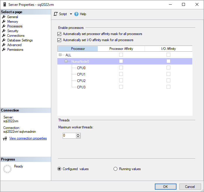
Figure 3-5 Set the affinity mask in SQL Server Management Studio.
By setting an affinity mask, you instruct SQL Server to use only specific cores. The remaining unused cores are marked as offline to SQL Server. When SQL Server starts, it will assign a scheduler to each online core.
Caution
Affinity masking is not a legitimate way to circumvent licensing limitations with SQL Server Standard edition. If you have more cores than the maximum usable by a certain edition, all logical cores on that machine must be licensed.
Configure affinity on Linux
For SQL Server on Linux, even when an instance is going to be using all the logical processors, you should use the ALTER SERVER CONFIGURATION option to set the PROCESS AFFINITY value. This value maintains efficient behavior between the Linux OS and the SQL Server Scheduler.
You can set the affinity by CPU or NUMA node, but the NUMA method is simpler. Suppose you have four NUMA nodes. You can use the configuration option to set the affinity to use all the NUMA nodes as follows:
ALTER SERVER CONFIGURATION SET PROCESS AFFINITY NUMANODE = 0 TO 3;- You can read more about best practices for configuring SQL Server on Linux at https://learn.microsoft.com/sql/linux/sql-server-linux-performance-best-practices.
File system configuration
This section primarily deals with the default file system on Windows Server. Any references to other file systems, including Linux file systems, are noted separately.
The NT File System (NTFS) was created for the first version of Windows NT, bringing with it more granular security than the older File Allocation Table (FAT)–based file system, as well as a journaling file system. (Think of it as a transaction log for your file system.) You can configure several settings that deal with NTFS in some way to improve your SQL Server implementation and performance.
Instant file initialization
As stated, transaction log files need to be zeroed out at the file system for recovery to work properly. However, data files are different, and with their 8-KB page size and allocation rules, the underlying file might contain sections of unused space.
With instant file initialization (IFI), a feature enabled by the Perform Volume Maintenance Tasks Active Directory policy, data files can be instantly resized without zeroing-out the underlying file. This adds a major performance boost.
The trade-off is a tiny, perhaps insignificant security risk: data that was previously used in drive allocation currently dedicated to a database’s data file now might not be fully erased before use. Because you can examine the underlying bytes in data pages using built-in tools in SQL Server, individual pages of data that have not yet been overwritten inside the new allocation could be visible to a malicious administrator.
Caution
It is important to control access to SQL Server’s data files and backups. When a database is in use by SQL Server, only the SQL Server service account and the local administrator have access. However, if the database is detached or backed up, there is an opportunity to view that deleted data on the detached file or backup file that was created with instant file initialization turned on.
Because this is a possible security risk, the Perform Volume Maintenance Tasks policy is not granted to the SQL Server service by default, and a summary of this warning is displayed during SQL Server setup.
Without IFI, you might find that the SQL Server wait type PREEMPTIVE_OS_WRITEFILEGATHER is prevalent during times of data-file growth. This wait type occurs when a file is being zero-initialized; thus, it can be a sign that your SQL Server is wasting time that could be skipped with the benefit of IFI. Keep in mind that PREEMPTIVE_OS_WRITEFILEGATHER is also generated by transaction log files, which do not benefit from IFI.
Note that SQL Server Setup takes a slightly different approach to granting this privilege than SQL Server administrators might take. SQL Server assigns access control lists (ACLs) to automatically created security groups, not to the service accounts that you select on the Server Configuration Setup page. Instead of granting the privilege to the named SQL Server service account directly, SQL Server grants the privilege to the per-service security identifier (SID) for the SQL Server database service—for example, the NT SERVICEMSSQLSERVER principal. This means that SQL Server service will maintain the ability to use IFI even if its service account changes.
You can determine whether the SQL Server Database Engine service has been granted access to IFI by using the sys.dm_server_services dynamic management view via the following query:
SELECT servicename, instant_file_initialization_enabled
FROM sys.dm_server_services
WHERE filename LIKE '%sqlservr.exe%';If IFI was not configured during SQL Server setup, and you want to do so later, open the Windows Start menu. Then, in the Search box, type Local Security Policy. In the pane on the left of the window that appears, expand Local Policies (see Figure 3-6); then select User Rights Assignment. Finally, locate the Perform Volume Maintenance Tasks policy and add the SQL Server service account to the list of objects with that privilege.
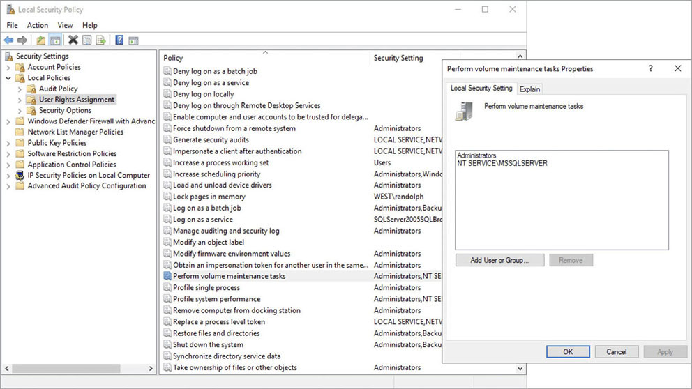
Figure 3-6 Turning on instant file initialization (IFI) through the Local Security Policy setup page.
NTFS allocation unit size
SQL Server performs best with an allocation unit size of 64 KB. Depending on the type of storage, the default allocation unit on NTFS might be 512 bytes, 4,096 bytes (also known as Advanced Format 4K sector size), or some other multiple of 512 bytes.
Because SQL Server deals with 64-KB extents (see the section “Group data pages with extents” earlier in the chapter), it performs best with an allocation unit size of 64 KB, to align the extents with the allocation units. This applies to the Resilient File System (ReFS) on Windows Server, and XFS and ext4 file systems on Linux.
Note
We cover aligned storage in more detail in Chapter 4 in the section “Important SQL Server volume settings.”