Chapter 8
Maintain and monitor SQL Server
Previous chapters covered the importance and logistics of database backups, but what else do you need to do on a regular basis to maintain a healthy SQL Server?
This chapter lays the foundation for the what and why of Microsoft SQL Server monitoring, based on dynamic management objects (DMOs), Database Consistency Checker (DBCC) commands, Extended Events (which replace Profiler/trace), and other tools provided by Microsoft.
Beyond simply setting up these tools, this chapter reviews what to look for on SQL Server instances on Windows and Linux, as well as SQL monitoring solutions in the Azure portal.
There is a lot for a DBA to be concerned with to monitor your databases—corrupt data files, lack of use of indexes and stats, properly sized data files, and baselined performance metrics, just to start. This chapter covers these topics and more.
All sample scripts in this book are available for download at https://MicrosoftPressStore.com/SQLServer2022InsideOut/downloads.
Detect, prevent, and respond to database corruption
After database backups, the second most important task concerning database integrity is proper configuration to prevent—and monitoring to mitigate—database corruption. A very large part of this is a proactive schedule of detection for rare cases when corruption occurs despite your best efforts. This isn’t a complicated topic and mostly revolves around configuring one setting and regularly running one command.
Set the database’s page verify option
For all databases, the page verify option should be CHECKSUM. Since SQL Server 2005, CHECKSUM has been the superior and default setting, but it requires a manual change after a database is restored up to a new SQL Server version.
If you still have databases whose page verify option is not CHECKSUM, you should change this setting immediately. The legacy NONE or TORN_PAGE_DETECTION options for this setting are a clear sign that this database has been moved over the years from a pre–SQL Server 2005 version. This setting is never automatically changed; you must change this setting after restoring the database up to a new version of SQL Server.
Warning
Before making the change to the CHECKSUM page verify option, take a full backup!
If corruption is found with the newly enabled CHECKSUM setting, the database can drop into a SUSPECT state, in which it becomes inaccessible. It is entirely possible that changing a database from NONE or TORN_PAGE_DETECTION to CHECKSUM could result in the discovery of existing, even long-present database corruption.
You should periodically run CHECKDB on all databases. This is a time-consuming but crucial process. You should run DBCC CHECKDB at least as often as your backup retention plan. Consider DBCC CHECKDB nearly as important as regular database backups.
The only reliable solution to database corruption is restoring from a known good backup.
For example, if you keep local backups around for one month, you should ensure that you perform a successful DBCC CHECKDB at least once per month, but more often is recommended. This ensures you will at least have a recovery point for uncorrupted, unchanged data, and a starting point for corrupted data fixes.
The DBCC CHECKDB command covers other more granular database integrity check tasks, including DBCC CHECKALLOC, DBCC CHECKTABLE, and DBCC CHECKCATALOG, all of which are important, and in only rare cases need to be run separately to split up the workload.
Running DBCC CHECKDB with no other parameters or syntax performs an integrity test on the current database context. Without specifying a database, however, no other additional options can be provided.
On large databases, DBCC CHECKDB is a resource-intensive operation (CPU, memory, and I/O), can take hours, and affects other user queries because of that resource consumption. DBCC CHECKDB may take hours to complete and tie up CPU resources, so it should be run only outside of business hours. To mitigate this, consider specifying the MAXDOP option (more on that in a moment). You can evaluate the progress of a DBCC CHECKDB operation (as well as backup and restore operations) by referencing the value in sys.dm_exec_requests.percent_complete for the executing session.
Here are some parameters worth noting:
NOINDEX. This can reduce the duration of the integrity check by skipping checks on nonclustered rowstore and columnstore indexes. It is not recommended.
Example usage:
DBCC CHECKDB (databasename, NOINDEX);REPAIR_REBUILD. This ensures you have no data loss. However, there are some limitations to its potential benefit. You should run this only after considering other options, including a backup and restore, because although it might have some success, it is unlikely to result in a complete repair. It can also be very time consuming, involving the rebuilding of indexes based on attempted repair data.
 Review the
 DBCC CHECKDBdocumentation at https://learn.microsoft.com/sql/t-sql/database-console-commands/dbcc-checkdb-transact-sql.
Example usage:
DBCC CHECKDB (databasename) WITH REPAIR_REBUILD;REPAIR_ALLOW_DATA_LOSS. You should run this only as a last resort to achieve a partial database recovery, because it can force a database to resolve errors by simply deallocating pages, potentially creating gaps in rows or columns. You must run this in
SINGLE_USERmode, and you should run it inEMERGENCYmode. Review theDBCC CHECKDBdocumentation for a number of caveats, and do not execute this command casually.Example usage (last resort only, not recommended!):
ALTER DATABASE WorldWideImporters SET EMERGENCY, SINGLE_USER;
DBCC CHECKDB('WideWorldImporters', REPAIR_ALLOW_DATA_LOSS);
ALTER DATABASE WorldWideImporters SET MULTI_USER;
Note
A complete review of
EMERGENCYmode andREPAIR_ALLOW_DATA_LOSSis detailed in this blog post by Microsoft’s originalDBCC CHECKDBengineer, Paul Randal: http://sqlskills.com/blogs/paul/checkdb-from-every-angle-emergency-mode-repair-the-very-very-last-resort.WITH NO_INFOMSGS. This suppresses informational status messages and returns only errors.
Example usage:
DBCC CHECKDB (databasename) WITH NO_INFOMSGS;WITH ESTIMATEONLY. This estimates the amount of space required in tempdb for the
CHECKDBoperation.Example usage:
DBCC CHECKDB (databasename) WITH ESTIMATEONLY;WITH MAXDOP = n. Similar to limiting the maximum degree of parallelism in other areas of SQL Server, this option limits the
CHECKDBoperation’s parallelism, possibly extending duration but potentially reducing the CPU utilization. SQL Server Enterprise edition supports parallel execution of theDBCC CHECKDBcommand, up to the server’sMAXDOPsetting. Therefore, in Enterprise edition, considerMAXDOP = 1to run the command single-threaded, or, overriding the other limitations on maximum degree of parallelism withMAXDOP = 0, allowing theCHECKDBunlimited parallelism to potentially finish sooner. Outside of Enterprise and Developer editions of SQL Server, objects are not checked in parallel.Example usage, combined with the aforementioned
NO_INFOMSGScommand to show multiple parameters:DBCC CHECKDB (databasename) WITH NO_INFOMSGS, MAXDOP = 0;- You can see all the syntax options for
CHECKDB, and those options that can be used together, at https://learn.microsoft.com/sql/t-sql/database-console-commands/dbcc-checkdb-transact-sql#syntax. - For more information on automating
DBCC CHECKDB, see Chapter 9, “Automate SQL Server administration.”
Repair database data file corruption
Of course, the only real remedy to data corruption after it has happened is to restore from a backup that predates the corruption. The well-documented DBCC CHECKDB option for REPAIR_ALLOW_DATA_LOSS, discussed previously, should be a last resort.
It is possible to repair missing pages in clustered indexes by piecing together missing columns in nonclustered indexes. If you are fortunate enough that corruption is only in nonclustered indexes, you can simply rebuild those indexes to recover from corruption. However, in many cases, clustered index or system pages are corrupt, meaning the only option is to restore the database. It is also possible to recover from data corruption, admittedly a lucky endeavor that this author has benefited from, by identifying the objects reported by DBCC CHECKDB and performing index rebuild operations on them.
Finally, availability groups provide a built-in data-corruption detection and automatic repair capability by using uncorrupted data on one replica to replace inaccessible data on another.
- For more information on this feature of availability groups, see Chapter 11, “Implement high availability and disaster recovery.”
Recover from database transaction log file corruption
In addition to following guidance in the previous chapter on the importance of backups, you can reconstitute a corrupted or lost database transaction log file by using the code that follows. A lost transaction log file could result in the loss of uncommitted data (or in the case of delayed durability tables, the loss of data that hasn’t been made durable in the log yet), but in the event of a disaster recovery involving the loss of the .ldf file with an intact .mdf file, this could be a valuable step.
It is possible to rebuild a blank transaction log file in a new file location for a database by using the following command:
ALTER DATABASE DemoDb SET EMERGENCY, SINGLE_USER;
ALTER DATABASE DemoDb REBUILD LOG
ON (NAME= DemoDb_Log, FILENAME = 'F:DATADemoDb_new.ldf');
ALTER DATABASE DemoDb SET MULTI_USER;
Note
Rebuilding a blank transaction log file using ALTER DATABASE … REBUILD LOG is not supported for databases containing a MEMORY_OPTIMIZED_DATA filegroup.
Database corruption in Azure SQL Database
Like many other administrative concerns with a platform as a service (PaaS) database, integrity checks for Azure SQL Database are automated. Microsoft takes data integrity in its PaaS database offering very seriously and provides strong assurances of assistance and recovery for this product. Albeit rare, Azure engineering teams respond 24×7 globally to data-corruption reports. The Azure SQL Database engineering team details its response promises at https://azure.microsoft.com/blog/data-integrity-in-azure-sql-database/.
Note
While Azure SQL Managed Instance has many PaaS-like qualities, automated integrity checks are not one of them. You should set up maintenance plans to execute DBCC CHECKDB, index maintenance, and other maintenance topics discussed in this chapter for Azure SQL Managed Instance.
- We discuss Azure SQL Managed Instance in detail in Chapter 18, “Provision Azure SQL Managed Instance.”
Maintain indexes and statistics
Index fragmentation occurs when insert, update, and delete activity occurs within tables, and there is not enough free space for that data, causing data to be split across pages. It can also happen when index pages get out of order, resulting in inefficient scans. Index fragmentation is caused by improper organization of rowstore data within the file that SQL Server maintains. Removing fragmentation is really about minimizing the number of pages that must be involved when queries read or write those data pages. Reducing fragmentation in database objects is vastly different from reducing fragmentation at the drive level, and has little in common with the Windows Disk Defragmenter application. Although this doesn’t translate to page locations on disk, and has even less relevance on storage area networks (SANs), it does translate to the activity of I/O systems when retrieving data.
In performance terms, the higher the amount of fragmentation (easily measurable in dynamic management views, as discussed later), the more activity is required for accessing the same amount of data.
The causes of index fragmentation are writes. Our data would stay nice and tidy if applications would stop writing to it! Updates and deletes will inevitably have a significant effect on clustered and nonclustered index fragmentation, plus the effect that inserts can have on fragmentation because of clustered index design.
The information in this section is largely unchanged from previous versions of SQL Server and applies to SQL Server instances, databases in Azure SQL Database, Azure SQL Managed Instance, and even dedicated SQL pools in Azure Synapse Analytics (formerly known as Azure SQL Data Warehouse).
Change the fill factor when beneficial
Each rowstore index on disk-based objects has a numeric property called a fill factor that specifies the percentage of space to be filled with rowstore data in each leaf-level data page of the index when it is created or rebuilt. The instance-wide default fill factor is 100 percent, which is represented by the setting value 0, and means that each leaf-level data page will be filled with as much data as possible. A fill factor setting of 80 (percent) means that 20 percent of leaf-level data pages will be intentionally left empty when data is inserted. You can adjust this fill factor percentage for each index to manage the efficiency of data pages.
A non-default fill factor may help reduce the number of page splits, which occur when the Database Engine attempts to add a new row of data or update an existing row with more data to a page that does not have enough space to add a new row. In this case, the Database Engine will clear out space for the new row by moving a proportion of the old rows to a new page. A page split can be a time-consuming and resource-consuming operation, with many page splits possible during writes, and will lead to index fragmentation.
However, setting a non-default fill factor will also increase the number of pages needed to store the same data and increase the number of reads needed for query operations. For example, a fill factor of 50 will roughly double the space on the drive that it initially takes to store and therefore access the data when compared to the default fill factor of 0.
In most instances, data is read far more often than it is written and inserted, updated, and deleted upon occasion. Indexes will therefore benefit from a high or default fill factor—usually more than 80—because it is almost always more important to keep the number of reads to a manageable level than to minimize the resources needed to perform a page split. You can deal with index fragmentation by using the REBUILD or REORGANIZE commands, as discussed in the next section.
If the key value for an index is constantly increasing, such as an autoincrementing IDENTITY or SEQUENCE-populated field as the first key of a clustered index, the data is added to the end of a data page and any gaps would not need to be filled. In the case of a table for which data is always inserted sequentially and never updated, changing the fill factor from the default may offer no advantage. Even after fine-tuning a fill factor, the benefit of reducing page splits might not be noticeable to write performance. The design of your database may affect your choice of fill factor—for example, if your clustered index key is a GUID, you may choose to lower the fill factor.
You can set a fill factor when an index is first created, or you can change it by using the ALTER INDEX ... REBUILD syntax, as discussed in the next section.
Note
The OPTIMIZE_FOR_SEQUENTIAL_KEY feature, introduced in SQL Server 2019, can further benefit IDENTITY and SEQUENCE-populated columns. For more on this recommended new feature, see Chapter 15, “Understand and design indexes.”
Track page splits
If you intend to fine-tune the fill factor for important tables to maximize the performance/storage space ratio, you can measure page splits in two ways: with a query on a DMV (discussed here), and with an Extended Event session (covered later in this chapter).
You can use the performance counter DMV to measure page splits in aggregate on Windows Server, as shown here:
SELECT * FROM sys.dm_os_performance_counters WHERE counter_name ='Page Splits/sec';The cntr_value increments whenever a page split is detected. This is a bit misleading because to calculate the page splits per second, you must sample the incrementing value twice and divide by the time difference between the samples. When viewing this metric in Performance Monitor, the calculation is done for you.
You can also track page_split events alongside statement execution by adding the page_split event to sessions such as the Transact-SQL (T-SQL) template in the Extended Events wizard. You’ll see an example of this later in this chapter, in the section “Use Extended Events to detect page splits.”
- Extended Events and the
sys.dm_os_performance_countersDMV are discussed in more detail later in this chapter in the section “Query performance metrics with DMVs.” This section also includes a sample session script to trackpage_splitevents.
Monitor index fragmentation
You can find the extent to which an index is fragmented by interrogating the sys.dm_db_index_physical_stats dynamic management function (DMF).
Unlike most DMVs, this function can have a significant impact on server performance because it can tax I/O. To query this DMF, you must be a member of the sysadmin server role or the db_ddladmin or db_owner database roles. Alternatively, you can grant the VIEW DATABASE STATE or VIEW SERVER STATE permissions. The sys.dm_db_index_physical_stats DMF is often joined to catalog views like sys.indexes or sys.objects, which require the user to have some permissions to the tables in addition to VIEW DATABASE STATE or VIEW SERVER STATE.
- For more information, visit https://learn.microsoft.com/sql/relational-databases/system-dynamic-management-views/sys-dm-db-index-physical-stats-transact-sql#permissions and https://learn.microsoft.com/sql/relational-databases/security/metadata-visibility-configuration.
Keep this in mind when scripting this operation for automated index maintenance. (We talk more about automating index maintenance in Chapter 9.)
Some of the following samples can be executed against the WideWorldImporters sample database. You can download then restore the WideWorldImporters-Full.bak file from this location: https://go.microsoft.com/fwlink/?LinkID=800630. For example, to find the fragmentation level of all indexes on the Sales.Orders table in the WideWorldImporters sample database, you can use a query such as the following:
USE WideWorldImporters;
SELECT
DB = db_name(s.database_id)
, [schema_name] = sc.name
, [table_name] = o.name
, index_name = i.name
, s.index_type_desc
, s.partition_number -- if the object is partitioned
, avg_fragmentation_pct = s.avg_fragmentation_in_percent
, s.page_count -- pages in object partition
FROM sys.indexes AS i
CROSS APPLY sys.dm_db_index_physical_stats
(DB_ID(),i.object_id,i.index_id, NULL, NULL) AS s
INNER JOIN sys.objects AS o ON o.object_id = s.object_id
INNER JOIN sys.schemas AS sc ON o.schema_id = sc.schema_id
WHERE i.is_disabled = 0
AND o.object_id = OBJECT_ID('Sales.Orders');
The sys.dm_db_index_physical_stats DMF accepts five parameters: database_id, object_id, index_id, partition_id, and mode. The mode parameter defaults to LIMITED, the fastest method, but you can set it to Sampled or Detailed. These additional modes are rarely necessary, but they provide more data, as well as more precise data. Some result set columns will be NULL in LIMITED mode. For the purposes of determining fragmentation, the default mode of LIMITED (used when the parameter value of NULL is provided or the literal LIMITED) suffices.
The five parameters of the sys.dm_db_index_physical_stats DMF are all nullable. For example, if you run the following script, you will see fragmentation statistics for all databases, objects, indexes, and partitions:
SELECT * FROM sys.dm_db_index_physical_stats(NULL,NULL,NULL,NULL,NULL);We recommend against executing this in a production environment during operational hours because, again, it can have a significant impact on server resources, resulting in a noticeable drop in performance.
Maintain indexes
After your automated script has identified the objects most in need of maintenance with the aid of sys.dm_db_index_physical_stats, it should proceed with steps to remove fragmentation in a timely fashion during a maintenance window. The commands to remove fragmentation are ALTER INDEX and ALTER TABLE, with REBUILD and REORGANIZE options. We explain the differences later, but briefly, rebuild is more thorough and potentially disruptive, whereas reorganize is less thorough, not disruptive, but often sufficient.
You must implement index maintenance for both rowstore and columnstore indexes; we cover strategies for both in this section.
Ideally, your automated index maintenance script runs as often as possible during regularly scheduled maintenance windows and for a limited amount of time. For example, if your business environment allows for a maintenance window each night between 1 a.m. and 4 a.m., try to run index maintenance each night in that window. If possible, modify your script to avoid starting new work after 4 a.m. or using the RESUMABLE PAUSE feature at 4 a.m. (More on the latter strategy in the upcoming section “Rebuild indexes.”) In databases with very large tables, index maintenance may require more time than you have within in a single maintenance window. Try to use the limited amount of time in each maintenance window with the greatest effect. Given ample time, this approach tends to work best to reduce fragmentation rather than, for example, a single very long maintenance period during a weekend. This feature also allows your active transaction log pages to be cleared with a log backup during the paused phases of an index rebuild.
- For more on maintenance plans and automating index maintenance, including the typical “care and feeding” of a SQL Server, see Chapter 9.
- For more on enabling the accelerated database recovery option, see Chapter 6, “Provision and configure SQL Server databases.”
Rebuild indexes
Performing an INDEX REBUILD operation on a rowstore index (clustered or nonclustered) physically re-creates the index B-tree leaf level. The goal of moving the pages is to make storage more efficient and to match the logical order provided by the index key. A rebuild operation is destructive to the index object and blocks other queries attempting to access the pages unless you provide the ONLINE option. Because the rebuild operation destroys and re-creates the index, it must update the index statistics afterward, eliminating the need to perform a subsequent UPDATE STATISTICS operation as part of regular maintenance.
Long-term table locks are held during the rebuild operation. One major advantage of SQL Server Enterprise edition remains the ability to specify the ONLINE option, which allows for rebuild operations that are significantly less disruptive to other queries, though not completely. This makes index maintenance feasible on SQL Servers with round-the-clock activity.
Consider using ONLINE with index rebuild operations whenever short maintenance windows are insufficient for rebuilding fragmented indexes offline. An online index rebuild, however, might take longer than an offline rebuild. There are also scenarios for which an online rebuild is not possible, including deprecated data types image, text, and ntext, or the xml data type. Since SQL Server 2012, it has been possible to perform ONLINE index rebuilds on the max lengths of the data types varchar, nvarchar, and varbinary.
For the syntax to rebuild the FK_Sales_Orders_CustomerID nonclustered index on the Sales.Orders table with the ONLINE functionality in Enterprise edition, see the following code sample:
ALTER INDEX FK_Sales_Orders_CustomerID
ON Sales.Orders
REBUILD WITH (ONLINE=ON);
It’s important to note that if you perform any kind of index maintenance on the clustered index of a rowstore table, it does not affect the nonclustered indexes. Nonclustered index fragmentation will not change if you rebuild the clustered index.
Instead of rebuilding each index on a table individually, you can rebuild all indexes on a table by replacing the name of the index with the keyword ALL. For example, to rebuild all indexes on the Sales.OrderLines table, do the following:
ALTER INDEX ALL ON [Sales].[OrderLines] REBUILD;This is usually overkill and inefficient, however, because not all indexes may have the same level of fragmentation or need for maintenance. Remember, we should perform index maintenance as granularly as possible.
For memory-optimized tables, we recommend a manual routine maintenance step using the ALTER TABLE … ALTER INDEX … REBUILD syntax. This is not to reduce fragmentation in the in-memory data; rather, it is to examine the number of buckets in a memory-optimized table’s hash indexes. For more information on rebuilding hash indexes and bucket counts, see Chapter 15.
Note
You can change the data compression option for indexes with the rebuild operation using the DATA_COMPRESSION option. For more detail on data compression, see Chapter 3, “Design and implement an on-premises database infrastructure.”
Aside from ONLINE, there are other options that you might want to consider for rebuild operations. Let’s look at them:
SORT_IN_TEMPDB. Use this when you want to create or rebuild an index using tempdb for sorting the index data, potentially increasing performance by distributing the I/O activity across multiple drives. This also means that these sorting worktables are written to the tempdb database transaction log instead of the user database transaction log, potentially reducing the impact on the user database log file, and allowing for the user database transaction log to be backed up during the operation.
MAXDOP. Use this to mitigate some of the impact of index maintenance by preventing the operation from using parallel processors. This can cause the operation to run longer, but to have less impact on performance.
WAIT_AT_LOW_PRIORITY. First introduced in SQL Server 2014, this is the first of a set of parameters that you can use to instruct the
ONLINEindex maintenance operation to try not to block other operations. This feature is known as Managed Lock Priority, and this syntax is not usable outside of online index operations and partition-switching operations. (SQL Server 2022 also introduced the ability to useWAIT_AT_LOW_PRIORITYforDBCC SHRINKDATABASEandDBCC SHRINKFILEoperations.) Here is the full syntax:ALTER INDEX PK_Sales_OrderLines on [Sales].[OrderLines] REBUILD WITH (ONLINE=ON (WAIT_AT_LOW_PRIORITY (MAX_DURATION = 5 MINUTES, ABORT_AFTER_WAIT = SELF)));The parameters for
MAX_DURATIONandABORT_AFTER_WAITinstruct the statement on how to proceed if it begins to be blocked by another operation. The online index operation will wait, allowing other operations to proceed.The
ABORT_AFTER_WAITparameter provides an action at the end of theMAX_DURATIONwait:SELFinstructs the statement to terminate its own process, ending the online rebuild step.BLOCKERSinstructs the statement to terminate the other process that is being blocked, terminating what is potentially a user transaction. Use with caution.NONEinstructs the statement to continue to wait. When combined withMAX_DURATION = 0, it is essentially the same behavior as not specifyingWAIT_AT_LOW_PRIORITY.
RESUMABLE. Introduced in SQL Server 2017, this feature makes it possible to initiate an online index creation or rebuild that can be paused and resumed later, even after a server shutdown. You can also specify a
MAX_DURATIONin minutes when starting an index rebuild operation, which will pause the operation if it exceeds the specified duration. You cannot specify theALLkeyword for a resumable operation. TheSORT_IN_TEMPDB=ONoption is not compatible with theRESUMABLEoption.
Note
Starting with SQL Server 2019, the RESUMABLE syntax can also be used when creating an index. An ALTER INDEX and CREATE INDEX statement can be similarly paused and resumed.
To leverage resumable index maintenance operations, you can see a list of resumable and paused index operations in a new DMV, sys.index_resumable_operations, where the state_desc field will reflect RUNNING (and pausable) or PAUSED (and resumable).
Here is a sample scenario of a paused/resumed index maintenance operation on a large table in the sample WideWorldImporters database:
ALTER INDEX PK_Sales_OrderLines on [Sales].[OrderLines]
REBUILD WITH (ONLINE = ON, RESUMABLE = ON);
From another session, show that the index rebuild is RUNNING with the RESUMABLE option:
SELECT object_name = object_name (object_id), *
FROM sys.index_resumable_operations;
From a third session, run the following to pause the operation:
ALTER INDEX PK_Sales_OrderLines on [Sales].[OrderLines] PAUSE;You can then show that the index rebuild is paused:
SELECT object_name = object_name (object_id), * FROM sys.index_resumable_operations;This sample is on a relatively small table, and may not allow you to execute the pause before the index rebuild is completed. This will result in a disconnection of the session of the original index maintenance, and a severe error message. In the SQL Server Error Log, the event is not a severe error message, but an informative note that “An ALTER INDEX ‘PAUSE’ was executed for….”
To resume the index maintenance operation, you have two options:
Reissue the same index maintenance operation, which will warn you it’ll just resume instead.
ALTER INDEX PK_Sales_OrderLines on [Sales].[OrderLines] REBUILD
WITH (ONLINE = ON, RESUMABLE = ON);
Issue a
RESUMEto the same index.ALTER INDEX PK_Sales_OrderLines on [Sales].[OrderLines] RESUME;
Reorganize indexes
Performing a REORGANIZE operation on an index uses fewer system resources and is much less disruptive than performing a full rebuild, while still accomplishing the goal of reducing fragmentation. It physically reorders the leaf-level pages of the index to match the logical order. It also compacts pages to match the fill factor on the index, though it does not allow the fill factor to be changed. This operation is always performed online, so long-term table locks (except for schema locks) are not held, and queries or modifications to the underlying table or index data will not be blocked by the schema lock during the REORGANIZE transaction.
Because the REORGANIZE operation is not destructive, it does not automatically update the statistics for the index afterward as a rebuild operation does. Thus, you should always follow a REORGANIZE step with an UPDATE STATISTICS step.
- For more on statistics objects and their impact on performance, see Chapter 15.
The following example presents the syntax to reorganize the PK_Sales_OrderLines index on the Sales.OrderLines table:
ALTER INDEX PK_Sales_OrderLines on [Sales].[OrderLines] REORGANIZE;None of the options available to rebuild that we covered in the previous section are available to the REORGANIZE command. The only additional option that is specific to REORGANIZE is the LOB_COMPACTION option. It compresses large object (LOB) data, which affects only LOB data types: image, text, ntext, varchar(max), nvarchar(max), varbinary(max), and xml. By default, this option is enabled, but you can disable it for non-heap tables to potentially skip some activity, though we do not recommend it. For heap tables, LOB data is always compacted.
Update index statistics
SQL Server uses statistics to describe the distribution and nature of the data in tables. The Query Optimizer needs the auto create setting enabled (it is enabled by default) so it can create single-column statistics when compiling queries. These statistics help the Query Optimizer create the most optimal query plans at runtime. The auto update statistics option prompts statistics to be updated automatically when accessed by a T-SQL query. This only occurs when the table is discovered to have passed a threshold of rows changed. Without relevant and up-to-date statistics, the Query Optimizer might not choose the best way to run queries.
An update of index statistics should accompany INDEX REORGANIZE steps to ensure that statistics on the table are current, but not INDEX REBUILD steps. Remember that the INDEX REBUILD command also updates the index statistics.
The basic syntax to update the statistics for an individual table is as follows:
UPDATE STATISTICS [Sales].[Invoices];The only command option to be aware of concerns the depth to which the statistics are scanned before being recalculated. By default, SQL Server samples a statistically significant number of rows in the table. This sampling is done with a parallel process starting with database compatibility level 150. This is fast and adequate for most workloads. You can optionally choose to scan the entire table by specifying the FULLSCAN option, or a sample of the table based on a percentage of rows or a fixed number of rows using the SAMPLE option, but these options are typically reserved for cases of unusual data skew where the default sampling may not provide adequate coverage for your column or index.
You can manually verify that indexes are being kept up to date by the Query Optimizer when auto_create_stats is enabled. The sys.dm_db_stats_properties DMF accepts an object_id and stats_id, which is functionally the same as the index_id, if the statistics object corresponds to an index. The sys.dm_db_stats_properties DMF returns information such as the modification_counter of rows changed since the last statistics update, and the last_updated date, which is NULL if the statistics object has never been updated since it was created.
Not all statistics are associated with an index, such as statistics that are automatically created. There will generally be more statistics objects than index objects. This function works in SQL Server and Azure SQL Database. You can easily tell if a statistics object (which you can gather from querying sys.stats) is automatically created by its naming convention, WA_Sys_<column_name>_<object_id_hex>, or by looking at the user_created and auto_created columns in the same view.
- For more on statistics objects and their impact on performance, see Chapter 15.
Reorganize columnstore indexes
You must also maintain columnstore indexes, but these use different internal objects to measure the fragmentation of the internal columnstore structure. Columnstore indexes need only the REORGANIZE operation. For more on designing columnstore indexes, see Chapter 15.
You can review the current structure of the groups of columnstore indexes by using the DMV sys.dm_db_column_store_row_group_physical_stats. This returns one row per row group of the columnstore structure. The state of a row group, and the current count of row groups by their states, provides some insight into the health of the columnstore index. Most row group states should be COMPRESSED. Row groups in the OPEN and CLOSED states are part of the delta store and are awaiting compression. These delta store row groups are served up alongside compressed data seamlessly when queries use columnstore data.
The number of deleted rows in a rowgroup is also an indication that the index needs maintenance. As the ratio of deleted rows to total rows in a row group that is in the COMPRESSED state increases, the performance of the columnstore index will be reduced. If delete_rows is larger than or greater than the total rows in a rowgroup, a REORGANIZE step will be beneficial.
Performing a REBUILD operation on a columnstore index is essentially the same as performing a drop/re-create and is not necessary. However, if you want to force the rebuild process, using the WITH (ONLINE = ON) syntax is supported starting with SQL Server 2019 for rebuilding (and creating) columnstore indexes. A REORGANIZE step for a columnstore index, just as for a nonclustered index, is an online operation that has minimal impact to concurrent queries.
You can also use the REORGANIZE WITH (COMPRESS_ALL_ROW_GROUPS=ON) option to force all delta store row groups to be compressed into a single compressed row group. This can be useful when you observe many compressed row groups with fewer than 100,000 rows.
Without COMPRESS_ALL_ROW_GROUPS, only compressed row groups will be compressed and combined. Typically, compressed row groups should contain up to one million rows each, but SQL might align rows in compressed row groups that align with how the rows were inserted, especially if they were inserted in bulk operations.
- We talk more about automating index maintenance in Chapter 9.
Manage database file sizes
It is important to understand the distinction between the size of a database data or log files, which act simply as reservations for SQL Server to work in, and the data within those reservations. Note that this section does not apply to Azure SQL Database, because this level of file management is not available and is automatically managed.
In SQL Server Management Studio (SSMS), you can right-click a database, select Reports, and choose Disk Usage to view the Disk Usage report for a database. It contains information about how much data is in the database’s files.
Alternatively, the following query uses the FILEPROPERTY function to reveal how much data there is inside a file reservation. We again use the undocumented but well-understood sp_msforeachdb stored procedure to iterate through each of the databases, accessing the sys.database_files catalog view.
DECLARE @FILEPROPERTY TABLE
( DatabaseName sysname
,DatabaseFileName nvarchar(500)
,FileLocation nvarchar(500)
,FileId int
,[type_desc] varchar(50)
,FileSizeMB decimal(19,2)
,SpaceUsedMB decimal(19,2)
,AvailableMB decimal(19,2)
,FreePercent decimal(19,2) );
INSERT INTO @FILEPROPERTY
exec sp_MSforeachdb 'USE [?];
SELECT
 Database_Name                   = d.name
, Database_Logical_File_Name     = df.name
, File_Location                  = df.physical_name
, df.File_ID
, df.type_desc
, FileSize_MB = CAST(size/128.0 as Decimal(19,2))
, SpaceUsed_MB = CAST(CAST(FILEPROPERTY(df.name, "SpaceUsed") AS int)/128.0 AS
decimal(19,2))
, Available_MB = CAST(size/128.0 - CAST(FILEPROPERTY(df.name, "SpaceUsed") AS int)/128.0
AS decimal(19,2))
, FreePercent = CAST((((size/128.0) - (CAST(FILEPROPERTY(df.name, "SpaceUsed") AS
int)*8/1024.0)) / (size*8/1024.0) ) * 100. AS decimal(19,2))
 FROM sys.database_files as df
 CROSS APPLY sys.databases as d
 WHERE d.database_id = DB_ID();'
SELECT * FROM @FILEPROPERTY
WHERE SpaceUsedMB is not null
ORDER BY FreePercent asc; --Find files with least amount of free space at top
Run this on a database in your environment to see how much data there is within database files. You might find that some data or log files are near full, whereas others have a large amount of space. Why would this be?
Files that have a large amount of free space might have grown in the past but have since been emptied out. If a transaction log in the full recovery model has grown for a long time without having a transaction log backup, the .ldf file will have grown unchecked. Later, when a transaction log backup is taken, causing the log to truncate, it will be nearly empty, but the size of the .ldf file itself will not have changed. It isn’t until you perform a shrink operation that the .ldf file will give its unused space back to the operating system (OS). In most cases, you should never shrink a data file, and certainly not on a schedule. The two main exceptions are if you mistakenly oversize a file or you applied data compression to a number of large database objects. In these cases, shrinking files as a one-time corrective action may be appropriate.
You should manually grow your database and log files to a size that is well ahead of the database’s growth pattern. You might fret over the best autogrowth rate, but ideally, autogrowth events are best avoided altogether by proactive file management.
Autogrowth events can be disruptive to user activity, causing all transactions to wait while the database file asks the OS for more space and grows. Depending on the performance of the I/O system, this could take seconds, during which activity on the database must wait. Depending on the autogrowth setting and the size of the write transactions, multiple autogrowth events could be suffered sequentially.
- Growth of database data files is also greatly sped up by instant file initialization, which is covered in Chapter 3.
Understand and find autogrowth events
You should change autogrowth rates for database data and log files from the initial (and far too small) default settings, but, more importantly, you should maintain enough free space in your data and log files so that autogrowth events do not occur. As a proactive DBA, you should monitor the space in database files and grow the files ahead of time, manually and outside of peak business hours.
You can view recent autogrowth events in a database via a report in SSMS or a T-SQL script (see the code example that follows). In SSMS, in Object Explorer, right-click the database name. Then, on the shortcut menu that opens, select Reports, select Standard Reports, and then select Disk Usage. An expandable/collapsible region of the report contains data/log files autogrow/autoshrink events.
The autogrowth report in SSMS reads data from the SQL Server instance’s default trace, which captures autogrowth events. This data is not captured by the default Extended Events session, called system_health, but you could capture autogrowth events with the sqlserver.database_file_size_change event in an Extended Event session.
To view and analyze autogrowth events more quickly, and for all databases simultaneously, you can query the SQL Server instance’s default trace yourself. The default trace files are limited to 20 MB, and there are at most five rollover files, yielding 100 MB of history. The amount of time this covers depends on server activity. The following sample code query uses the fn_trace_gettable() function to open the default trace file in its current location:
SELECT
DB = g.DatabaseName
, Logical_File_Name = mf.name
, Physical_File_Loc = mf.physical_name
, mf.type
-- The size in MB (converted from the number of 8-KB pages) the file increased.
, EventGrowth_MB = convert(decimal(19,2),g.IntegerData*8/1024.)
, g.StartTime --Time of the autogrowth event
-- Length of time (in seconds) necessary to extend the file.
, EventDuration_s = convert(decimal(19,2),g.Duration/1000./1000.)
, Current_Auto_Growth_Set = CASE
WHEN mf.is_percent_growth = 1
 THEN CONVERT(char(2), mf.growth) + '%'
 ELSE CONVERT(varchar(30), mf.growth*8./1024.) + 'MB'
END
, Current_File_Size_MB = CONVERT(decimal(19,2),mf.size*8./1024.)
, d.recovery_model_desc
FROM fn_trace_gettable(
(select substring((SELECT path
FROM sys.traces WHERE is_default =1), 0, charindex('log_',
(SELECT path FROM sys.traces WHERE is_default =1),0)+4)
+ '.trc'), DEFAULT) AS [g]
INNER JOIN sys.master_files mf
ON mf.database_id = g.DatabaseID
AND g.FileName = mf.name
INNER JOIN sys.databases d
ON d.database_id = g.DatabaseID
ORDER BY StartTime desc;
Understanding autogrowth events helps explain what happens to database files when they don’t have enough space. They must grow, or transactions cannot be accepted. What about the opposite scenario, where a database file has “too much” space? We cover that next.
Shrink database files
We need to be as clear as possible about this: Shrinking database files is not something that you should do regularly or casually. If you find yourself every morning shrinking a database file that grew overnight, stop. Think. Isn’t it just going to grow again tonight?
One of the main concerns with shrinking a file is that it indiscriminately returns free pages to the OS, helping to create fragmentation. Aside from potentially ensuring autogrowth events in the future, shrinking a file creates the need for further index maintenance to alleviate the fragmentation. A shrink step can be time consuming, can block other user activity, and is not part of a healthy complete maintenance plan.
Database data and logs under normal circumstances—and in the case of the full recovery model with regular transaction log backups—grow to the size they need to be because of actual usage. Frequent autogrowth events and shrink operations are bad for performance and create fragmentation.
To increase concurrency of shrink operations, by allowing DBCC SHRINKDATABASE and DBCC SHRINKFILE to patiently wait for locks, SQL Server 2022 introduces the WAIT_AT_LOW_PRIORITY syntax. This same keyword has similar application for online index maintenance commands and behaves similarly. When you specify WAIT_AT_LOW_PRIORITY, the shrink operation waits until it can claim the shared schema (Sch-S) and shared metadata (Sch-M) locks it needs. Other queries won’t be blocked until the shrink can actually proceed, resulting in less potential for blocked queries. The WAIT_AT_LOW_PRIORITY option is less configurable for the two shrink commands, and is hard-coded to a 1-minute timeout. If after 1 minute the shrink operation cannot obtain the necessary locks to proceed, it will be cancelled.
Shrink data files
Try to proactively grow database files to avoid autogrowth events altogether. You should shrink a data file only as a one-time event to solve one of three scenarios:
A drive volume is out of space and, in an emergency break-fix scenario, you reclaim unused space from a database data or log file.
A database transaction log grew to a much larger size than is normally needed because of an adverse condition and should be reduced back to its normal operating size. An adverse condition could be a transaction log backup that stopped working for a timespan, a large uncommitted transaction, or a replication availability group issue that prevented the transaction log from truncating.
For the rare situation in which a database had a large amount of data deleted from the file, an amount of data that is unlikely ever to exist in the database again, a one-shrink file operation might be appropriate.
Shrink transaction log files
For the case in which a transaction log file should be reduced in size, the best way to reclaim the space and re-create the file with optimal virtual log file (VLF) alignment is to first create a transaction log backup to truncate the log file as much as possible. If transaction log backups have not recently been generated on a schedule, it may be necessary to create another transaction log backup to fully clear out the log file. Once empty, shrink the log file to reclaim all unused space, then immediately grow the log file back to its expected size in increments of no more than 8,000 MB at a time. This allows SQL Server to create the underlying VLF structures in the most efficient way possible.
- For more information on VLFs in your database log files, see Chapter 3.
The following sample script of this process assumes a transaction log backup has already been generated to truncate the database transaction log and that the database log file is mostly empty. It also grows the transaction log file backup to 9 GB (9,216 MB or 9,437,184 KB). Note the intermediate step of growing the file first to 8,000 MB, then to its intended size.
USE [WideWorldImporters];
--TRUNCATEONLY returns all free space to the OS
DBCC SHRINKFILE (N'WWI_Log' , 0, TRUNCATEONLY);
GO
USE [master];
ALTER DATABASE [WideWorldImporters]
MODIFY FILE ( NAME = N'WWI_Log', SIZE = 8192000KB );
ALTER DATABASE [WideWorldImporters]
MODIFY FILE ( NAME = N'WWI_Log', SIZE = 9437184KB );
GO
Caution
You should never enable the autoshrink database setting. It automatically returns any free space of more than 25 percent of the data file or transaction log. You should shrink a database only as a one-time operation to reduce file size after unplanned or unusual file growth. This setting could result in unnecessary fragmentation, overhead, and frequent rapid log autogrowth events. This setting was originally intended, and might only be appropriate, for tiny local and/or embedded databases.
Monitor activity with DMOs
SQL Server provides a suite of internal dynamic management objects (DMOs) in the form of views (DMVs) and functions (DMFs). It is important for you as a DBA to have a working knowledge of these objects because they unlock the analysis of SQL Server outside of built-in reporting capabilities and third-party tools. In fact, third-party tools that monitor SQL Server almost certainly use these very dynamic management objects.
DMO queries are discussed in several other places in this book:
Chapter 14 discusses reviewing, aggregating, and analyzing cached execution plan statistics, including the Query Store feature introduced in SQL Server 2016.
Chapter 14 also discusses reporting from DMOs and querying performance monitor metrics within SQL Server DMOs.
Chapter 15 covers index usage statistics and missing index statistics.
Chapter 11 details high availability and disaster recovery features like automatic seeding.
The section “Monitor index fragmentation” earlier in this chapter talked about using a DMF to query index fragmentation.
Observe sessions and requests
Any connection to a SQL Server instance is a session and is reported live in the DMV sys.dm_exec_sessions. Any actively running query on a SQL Server instance is a request and is reported live in the DMV sys.dm_exec_requests. Together, these two DMVs provide a thorough and far more detailed replacement for the sp_who or sp_who2 system stored procedures, as well as the deprecated sys.sysprocesses system view, with which longtime DBAs might be more familiar. With DMVs, you can do so much more than replace sp_who.
By adding a handful of other DMOs, we can turn this query into a wealth of live information, including:
Complete connection source information
The actual runtime statement currently being run (like
DBCC INPUTBUFFER, but not limited to 254 characters)The actual plan XML (provided with a blue hyperlink in the SSMS results grid)
Request duration
Cumulative resource consumption
The current and most recent wait types experienced
Sure, it might not be as easy to type in as sp_who2, but it provides much more data, which you can easily query and filter. Save this as a go-to script in your personal DBA tool belt. If you are unfamiliar with any of the data being returned, take some time to dive into the result set and explore the information it provides; it will be an excellent hands-on learning resource. You might choose to add more filters to the WHERE clause specific to your environment. Let’s take a look:
SELECT
 when_observed = sysdatetime()
, s.session_id, r.request_id
, session_status = s.[status] -- running, sleeping, dormant, preconnect
, request_status = r.[status] -- running, runnable, suspended, sleeping, background
, blocked_by = r.blocking_session_id
, database_name = db_name(r.database_id)
, s.login_time, r.start_time
, query_text = CASE
 WHEN r.statement_start_offset = 0
 and r.statement_end_offset= 0 THEN left(est.text, 4000)
 ELSE SUBSTRING (est.[text], r.statement_start_offset/2 + 1,
 CASE WHEN r.statement_end_offset = -1
    THEN LEN (CONVERT(nvarchar(max), est.[text]))
    ELSE r.statement_end_offset/2 - r.statement_start_offset/2 + 1
 END
) END --the actual query text is stored as nvarchar,
--so we must divide by 2 for the character offsets
, qp.query_plan
, cacheobjtype = LEFT (p.cacheobjtype + ' (' + p.objtype + ')', 35)
, est.objectid
, s.login_name, s.client_interface_name
, endpoint_name = e.name, protocol = e.protocol_desc
, s.host_name, s.program_name
, cpu_time_s = r.cpu_time, tot_time_s = r.total_elapsed_time
, wait_time_s = r.wait_time, r.wait_type, r.wait_resource, r.last_wait_type
, r.reads, r.writes, r.logical_reads --accumulated request statistics
FROM sys.dm_exec_sessions as s
LEFT OUTER JOIN sys.dm_exec_requests as r on r.session_id = s.session_id
LEFT OUTER JOIN sys.endpoints as e ON e.endpoint_id = s.endpoint_id
LEFT OUTER JOIN sys.dm_exec_cached_plans as p ON p.plan_handle = r.plan_handle
OUTER APPLY sys.dm_exec_query_plan (r.plan_handle) as qp
OUTER APPLY sys.dm_exec_sql_text (r.sql_handle) as est
LEFT OUTER JOIN sys.dm_exec_query_stats as stat on stat.plan_handle = r.plan_handle
AND r.statement_start_offset = stat.statement_start_offset
AND r.statement_end_offset = stat.statement_end_offset
WHERE 1=1 --Veteran trick that makes for easier commenting of filters
AND s.session_id >= 50 --retrieve only user spids
AND s.session_id <> @@SPID --ignore this session
ORDER BY r.blocking_session_id desc, s.session_id asc;
Notice that the preceding script returned wait_type and last_wait_type. Let’s dive into these important performance signals now.
Understand wait types and wait statistics
Wait statistics in SQL Server are an important source of information and can be a key resource for finding bottlenecks in performance at the aggregate level and at the individual query level. A wait is a signal recorded by SQL Server indicating what SQL Server is waiting on when attempting to finish processing a query. This section provides insights into this broad and important topic. However, entire books, training sessions, and software packages have been developed to address wait type analysis.
Wait statistics can be queried and provide value to SQL Server instances as well as databases in Azure SQL Database and Azure SQL Managed Instance, though there are some waits specific to the Azure SQL Database platform (which we’ll review). Like many DMOs, membership in the sysadmin server role is not required, only the permission VIEW SERVER STATE, or in the case of Azure SQL Database, VIEW DATABASE STATE.
You saw in the query in the previous section the ability to see the current and most recent wait type for a session. Let’s dive into how to observe wait types in the aggregate, accumulated at the server level or at the session level. Waits can occur when a request is in the runnable or suspended state. SQL Server can track many different wait types for a single query, many of which are of negligible duration or are benign in nature. There are quite a few waits that can be ignored or that indicate idle activity, as opposed to waits that indicate resource constraints and blocking. There are more than 1,000 distinct wait types in SQL Server 2022 and even more in Azure SQL Database. Some are better documented and understood than others. We review some that you should know about later in this section.
- You can see the complete list of wait types at https://learn.microsoft.com/sql/relational-databases/system-dynamic-management-views/sys-dm-os-wait-stats-transact-sql#WaitTypes.
Monitor wait type aggregates
To view accumulated waits for a session, which live only until the close or reset of the session, use the sys.dm_exec_session_wait_stats DMV.
In sys.dm_exec_sessions, you can see the current wait type and most recent wait type, but this isn’t always that interesting or informative. Potentially more interesting would be to see all the accumulated wait stats for an ongoing session. This code sample shows how the DMV returns one row per session, per wait type experienced, for user sessions:
SELECT * FROM sys.dm_exec_session_wait_stats
ORDER BY wait_time_ms DESC;
There is a distinction between the two time measurements in this query and others. The value from signal_wait_time_ms indicates the amount of time the thread waited on CPU activity, correlated with time spent in the runnable state. The wait_time_ms value indicates the accumulated time in milliseconds for the wait type, including the signal_wait_time_ms, and so includes time the request spent in the runnable and suspended states. Typically, wait_time_ms is the wait measurement that we aggregate. The waiting_tasks_count is also informative, indicating the number of times this wait_type was encountered. By dividing wait_time_ms by waiting_tasks_count, you can get an average number of milliseconds (ms) each task encountered this wait.
You can view aggregate wait types at the instance level with the sys.dm_os_wait_stats DMV. This is the same as sys.dm_exec_session_wait_stats, but without the session_id, which includes all activity in the SQL Server instance without any granularity to database, query, time frame, and so on. This can be useful for getting the “big picture,” but it is limited over long spans of time because the wait_time_ms counter accumulates, as illustrated here:
SELECT TOP (25)
 wait_type
, wait_time_s = wait_time_ms / 1000.
, Pct = 100. * wait_time_ms/nullif(sum(wait_time_ms) OVER(),0)
, avg_ms_per_wait = wait_time_ms / nullif(waiting_tasks_count,0)
FROM sys.dm_os_wait_stats as wt ORDER BY Pct DESC;
Eventually, the wait_time_ms numbers will be so large for certain wait types that trends or changes in wait type accumulations rates will be mathematically difficult to see. You want to use the wait stats to keep a close eye on server performance as it trends and changes over time, so you need to capture these accumulated wait statistics in chunks of time, such as one day or one week.
--Script to set up capturing these statistics over time
CREATE TABLE dbo.usr_sys_dm_os_wait_stats
(   id int NOT NULL IDENTITY(1,1)
,   datecapture datetimeoffset(0) NOT NULL
,   wait_type nvarchar(512) NOT NULL
,   wait_time_s decimal(19,1) NOT NULL
,   Pct decimal(9,1) NOT NULL
,   avg_ms_per_wait decimal(19,1) NOT NULL
,   CONSTRAINT PK_sys_dm_os_wait_stats PRIMARY KEY CLUSTERED (id)
);
--This part of the script should be in a SQL Agent job, run regularly
INSERT INTO
Dbo.usr_sys_dm_os_wait_stats
(datecapture, wait_type, wait_time_s, Pct, avg_ms_per_wait)
SELECT
datecapture = SYSDATETIMEOFFSET()
, wait_type
, wait_time_s = convert(decimal(19,1), round( wait_time_ms / 1000.0,1))
, Pct = wait_time_ms/ nullif(sum(wait_time_ms) OVER(),0)
, avg_ms_per_wait = wait_time_ms / nullif(waiting_tasks_count,0)
FROM usr_sys.dm_os_wait_stats wt
WHERE wait_time_ms > 0
ORDER BY wait_time_s;
Using the metrics returned in the preceding code, you can calculate the difference between always-ascending wait times and counts to determine the counts between intervals. You can customize the schedule for this data to be captured in tables, building your own internal wait stats reporting table.
The sys.dm_os_wait_stats DMV is reset—and all accumulated metrics are lost—upon restart of the SQL Server service, but you can also clear them manually. Understandably, this would clear the statistics for the whole SQL Server instance. Here is a sample script of how you can capture wait statistics at any interval:
DBCC SQLPERF ('sys.dm_os_wait_stats', CLEAR);You can also view statistics for a query currently running in the DMV sys.dm_os_waiting_tasks, which contains more data than simply the wait_type; it also shows the blocking resource address in the resource_description field. This data is also available in sys.dm_exec_requests.
- For a complete breakdown of the information that can be contained in the
resource_descriptionfield, see http://learn.microsoft.com/sql/relational-databases/system-dynamic-management-views/sys-dm-os-waiting-tasks-transact-sql.
The query storage also tracks aggregated wait statistics for queries that it tracks. The waits tracked by the Query Store are not as detailed as the DMVs, but they do give you a quick idea of what a query is waiting on.
- For more information on reviewing waits in the Query Store, see Chapter 14.
Understand wait resources
What if you observe a query wait occurring live, and want to figure out what data the query is actually waiting on?
SQL Server 2019 delivered some new tools to explore the archaeology involved in identifying the root of waits. While an exhaustive look at the different wait resource types—some more cryptic than others—is best documented in Microsoft’s online resources, let’s review the tools provided.
The undocumented DBCC PAGE command (and its accompanying Trace Flag 3604) were used for years to review the information contained in a page, based on a specific page number. Whether trying to see the data at the source of waits or trying to peek at corrupted pages reported by DBCC CHECKDB, the DBCC PAGE command didn’t return any visible data without first enabling Trace Flag 3604. Now, for some cases, we have the pair of new functions, sys.dm_db_page_info and sys.fn_PageResCracker. Both can be used only when the sys.dm_exec_requests.wait_resource value begins with PAGE. So, the new tools leave out other common wait_resource types like KEY.
The DMVs in SQL Server 2019 and SQL Server 2022 are preferable to using DBCC PAGE because they are fully documented and supported. They can be combined with sys.dm_exec_requests—the hub DMV for all things active in SQL Server—to return potentially useful information about the object in contention when PAGE blocking is present:
SELECT r.request_id, pi.database_id, pi.file_id, pi.page_id, pi.object_id,
pi.page_type_desc, pi.index_id, pi.page_level, rows_in_page = pi.slot_count
FROM sys.dm_exec_requests AS r
CROSS APPLY sys.fn_PageResCracker (r.page_resource) AS prc
CROSS APPLY sys.dm_db_page_info(r.database_id, prc.file_id, prc.page_id, 'DETAILED') AS
pi;
Benign wait types
Many of the waits in SQL Server do not affect the performance of user workload. These waits are commonly referred to as benign waits and are frequently excluded from queries analyzing wait stats. The following code contains a starter list of wait types that you can mostly ignore when querying the sys.dm_os_wait_stats DMV for aggregate wait statistics. You can append the following sample list WHERE clause.
SELECT * FROM sys.dm_os_wait_stats
WHERE
    wt.wait_type NOT LIKE '%SLEEP%' --can be safely ignored, sleeping
AND wt.wait_type NOT LIKE 'BROKER%' -- internal process
AND wt.wait_type NOT LIKE '%XTP_WAIT%' -- for memory-optimized tables
AND wt.wait_type NOT LIKE '%SQLTRACE%' -- internal process
AND wt.wait_type NOT LIKE 'QDS%' -- asynchronous Query Store data
AND wt.wait_type NOT IN ( -- common benign wait types
'CHECKPOINT_QUEUE'
,'CLR_AUTO_EVENT','CLR_MANUAL_EVENT' ,'CLR_SEMAPHORE'
,'DBMIRROR_DBM_MUTEX','DBMIRROR_EVENTS_QUEUE','DBMIRRORING_CMD'
,'DIRTY_PAGE_POLL'
,'DISPATCHER_QUEUE_SEMAPHORE'
,'FT_IFTS_SCHEDULER_IDLE_WAIT','FT_IFTSHC_MUTEX'
,'HADR_FILESTREAM_IOMGR_IOCOMPLETION'
,'KSOURCE_WAKEUP'
,'LOGMGR_QUEUE'
,'ONDEMAND_TASK_QUEUE'
,'REQUEST_FOR_DEADLOCK_SEARCH'
,'XE_DISPATCHER_WAIT','XE_TIMER_EVENT'
--Ignorable HADR waits
, 'HADR_WORK_QUEUE'
,'HADR_TIMER_TASK'
,'HADR_CLUSAPI_CALL');
Through your own research into your workload, and in future versions of SQL Server, as more wait types are added, you can grow this list so that important and actionable wait types rise to the top of your queries. A prevalence of these wait types shouldn’t be a concern; they’re unlikely to be generated by or negatively affect user requests.
Wait types to be aware of
This section shouldn’t be the start and end of your understanding of or research into wait types. Many of them have multiple avenues to explore in your SQL Server instance, or at the very least, names that are misleading to the DBA considering their origin. There are some, or groups of some, that you should understand, because they indicate a condition worth investigating. Many wait types are always present in all applications but become problematic when they appear in large frequency and/or with large cumulative waits. Large here is of course relative to your workload and your server.
Different instance workloads will have a different profile of wait types. Just because a wait type is at the top of the aggregate sys.dm_os_wait_stats list, it doesn’t mean that is the main or only performance problem with a SQL Server instance. It is likely that all SQL Server instances, even finely tuned instances, will show these wait types near the top of the aggregate waits list. You should track and trend these wait stats, perhaps using the script example in the previous section.
Important waits include the following, provided in alphabetical order:
ASYNC_NETWORK_IO. This wait type is associated with the retrieval of data to a client (including SQL Server Management Studio and Azure Data Studio), and the wait while the remote client receives and finally acknowledges the data received. This wait almost certainly has very little to do with network speed, network interfaces, switches, or firewalls. Any client, including your workstation or even SSMS running locally on the server, can incur small amounts of
ASYNC_NETWORK_IOas data is retrieved to be processed. Transactional and snapshot replication distribution will incurASYNC_NETWORK_IO. You will see a large amount ofASYNC_NETWORK_IOgenerated by reporting applications such as Tableau, SSRS, SQL Server Profiler, and Microsoft Office products. The next time a rudimentary Access database application tries to load the entire contents of theSales.OrderLinestable, you’ll likely seeASYNC_NETWORK_IO.Reducing
ASYNC_NETWORK_IO, like many of the waits we discuss in this chapter, has little to do with hardware purchases or upgrades; rather, it’s more to do with poorly designed queries and applications. The solution, therefore, would be an application change. Try suggesting to developers or client applications incurring large amounts ofASYNC_NETWORK_IOthat they eliminate redundant queries, use server-side filtering as opposed to client-side filtering, use server-side data paging as opposed to client-side data paging, or use client-side caching.CXPACKET. A common and often-overreacted-to wait type,
CXPACKETis a parallelism wait. In a vacuum, execution plans that are created with parallelism run faster. But at scale, with many execution plans running in parallel, the server’s resources might take longer to process the requests. This wait is measured in part asCXPACKETwaits.When the
CXPACKETwait is the predominant wait type experienced over time by your SQL Server, you should consider turning both the Maximum Degree of Parallelism (MAXDOP) and Cost Threshold for Parallelism (CTFP) dials when performance tuning. Make these changes in small, measured gestures, and don’t overreact to performance problems with a small number of queries. Use the Query Store to benchmark and trend the performance of high-value and high-cost queries as you change configuration settings.If large queries are already a problem for performance and multiple large queries regularly run simultaneously, raising the
CTFPmight not solve the problem. In addition to the obvious solutions of query tuning and index changes, including the creation of columnstore indexes, useMAXDOPas well to limit parallelization for very large queries.Until SQL Server 2016,
MAXDOPwas either a setting at the server level, a setting enforced at the query level, or a setting enforced to sessions selectively via Resource Governor (more on this toward the end of this chapter in the section “Protect important workloads with Resource Governor”). Since SQL Server 2016, theMAXDOPsetting has been available as a database-scoped configuration. You can also use the MAXDOP query hint in any statement to override the database or server-levelMAXDOPsetting.
IO_COMPLETION. This wait type is associated with synchronous read and write operations that are not related to row data pages, such as reading log blocks or virtual log file (VLF) information from the transaction log, or reading or writing merge join operator results, spools, and buffers to disk. It is difficult to associate this wait type with a single activity or event, but a spike in
IO_COMPLETIONcould be an indication that these same events are now waiting on the I/O system to complete.LCK_M_*. Lock waits have to do with blocking and concurrency (or lack thereof). (Chapter 14 looks at isolation levels and concurrency.) When a request is writing and another request in
READ COMMITTEDor higher isolation is trying to lock that same row data, one of the 60+ differentLCK_M_*wait types will be the reported wait type of the blocked request. For example,LCK_M_ISmeans that the thread wants to acquire an Intent Shared lock, but some other thread has it locked in an incompatible manner.In the aggregate, this doesn’t mean you should reduce the isolation level of your transactions. Whereas
READ UNCOMMITTEDis not a good solution, read committed snapshot isolation (RCSI) and snapshot isolation are good solutions; see Chapter 14 for more details. Rather, you should optimize execution plans for efficient access, for example, by reducing scans as well as avoiding long-running multistep transactions. Also, avoid index rebuild operations without theONLINEoption. (See the “Rebuild indexes” section earlier in this chapter for more information.)The
wait_resourceprovided insys.dm_exec_requests, orresource_descriptioninsys.dm_os_waiting_tasks, provide a map to the exact location of the lock contention inside the database.- For a complete breakdown of the information that can be contained in the
resource_descriptionfield in your version of SQL Server, visit https://learn.microsoft.com/sql/relational-databases/system-dynamic-management-views/sys-dm-os-waiting-tasks-transact-sql.
MEMORYCLERK_XE. The
MEMORYCLERK_XEwait type could spike if you have allowed Extended Events session targets to consume too much memory. We discuss Extended Events later in this chapter, but you should watch out for the maximum buffer size allowed to thering_buffersession target, among other in-memory targets.OLEDB. This self-explanatory wait type describes waits associated with long-running external communication via the OLE DB provider, which is commonly used by SQL Server Integration Services (SSIS) packages, Microsoft Office applications (including querying Excel files), linked servers using the OLE DB provider, and third-party tools. It could also be generated by internal commands like
DBCC CHECKDB. When you observe this wait occurring in SQL Server, in most cases, it’s driven by long-running linked server queries.
PAGELATCH_* and PAGEIOLATCH_*. These two wait types are presented together not because they are similar in nature—they are not—but because they are often confused. To be clear,
PAGELATCHhas to do with contention over pages in memory, whereasPAGEIOLATCHrelates to contention over pages in the I/O system (on the drive).PAGELATCH_*contention deals with pages in memory, which can rise because of the overuse of temporary objects in memory, potentially with rapid access to the same temporary objects. This can also be experienced when reading in data from an index in memory or reading from a heap in memory.A rise in
PAGEIOLATCH_*could be due to the performance of the storage system (keeping in mind that the performance of drive systems does not always respond linearly to increases in activity). Aside from throwing (a lot of!) money at faster drives, a more economical solution is to modify queries and/or indexes and reduce the footprint of memory-intensive operations, especially operations involving index and table scans.PAGEIOLATCH_*contention has to do with a far more limiting and troubling performance condition: the overuse of reading from the slowest subsystem of all, the physical drives.PAGEIOLATCH_SHdeals with reading data from a drive into memory so that the data can be accessed. Keep in mind that this doesn’t necessarily translate to a request’s row count, especially if index or table scans are required in the execution plan.PAGEIOLATCH_EXandPAGEIOLATCH_UPare waits associated with reading data from a drive into memory so that the data can be written to.
RESOURCE_SEMAPHORE. This wait type is accumulated when a request is waiting on memory to be allocated before it can start. Although this could be an indication of memory pressure caused by insufficient memory available to process the queries being executed, it is more likely caused by poor query design and poor indexing, resulting in inefficient execution plans. Aside from throwing money at more system memory, a more economical solution is to tune queries and reduce the footprint of memory-intensive operations. The memory grant feedback features that are part of Intelligent Query Processing help address these waits by improving memory grants for subsequent executions of a query.
SOS_SCHEDULER_YIELD. Another flavor of CPU pressure, and in some ways the opposite of the
CXPACKETwait type, is theSOS_SCHEDULER_YIELDwait type. TheSOS_SCHEDULER_YIELDis an indicator of CPU pressure, indicating that SQL Server had to share time with, or yield to, other CPU tasks, which can be normal and expected on busy servers. WhereasCXPACKETis SQL Server complaining about too many threads in parallel,SOS_SCHEDULER_YIELDis the acknowledgement that there were more runnable tasks for the available threads. In either case, first take a strategy of reducing CPU-intensive queries and rescheduling or optimizing CPU-intense maintenance operations. This is more economical than simply adding CPU capacity.WAIT_XTP_RECOVERY. This wait type can occur when a database with memory-optimized tables is in recovery at startup and is expected. As with all wait types on performance-sensitive production SQL Server instances, you should baseline and measure it, but be aware this is not usually a sign of any problem.
WRITELOG. The
WRITELOGwait type is likely to appear on any SQL Server instance, including availability group primary and secondary replicas, when there is heavy write activity. TheWRITELOGwait is time spent flushing the transaction log to a drive and is due to physical I/O subsystem performance. On systems with heavy writes, this wait type is expected.You could consider re-creating the heavy-write tables as memory-optimized tables to increase the performance of writes. Memory-optimized tables optionally allow for delayed durability, which would resolve a bottleneck writing to the transaction log by using a memory buffer. For more information, see Chapter 14.
XE_FILE_TARGET_TVF and XE_LIVE_TARGET_TVF. These waits are associated with writing Extended Events sessions to their targets. A sudden spike in these waits would indicate that too much is being captured by an Extended Events session. Usually these aren’t a problem, because the asynchronous nature of Extended Events has a much lower impact than traces.
Monitor with the SQL Assessment API
The SQL Assessment API is a code-delivered method for programmatically evaluating SQL Server instance and database configuration. First introduced with SQL Server Management Objects (SMO) and the SqlServer PowerShell module in 2019, calls to the API can be used to evaluate alignment with best practices, and then can be scheduled to monitor regularly for variance.
You can use this API to assess SQL Servers starting with SQL Server 2012, for SQL Server on Windows and Linux. The assessment is performed by comparing SQL Server configuration to rules, stored as JSON files. Microsoft has provided a standard array of rules.
- Review the default JSON configuration file at https://learn.microsoft.com/sql/tools/sql-assessment-api/sql-assessment-api-overview.
Use this standard JSON file as a template to assess your own best practices if you like. The assessment configuration files are organized into the following:
Probes. These usually contain a T-SQL query—for example, to return data from DMOs (discussed earlier in this chapter). You can also write probes against your own user tables to query for code-driven states or statuses that can be provided by applications, ETL packages, or custom error-handling.
Checks. These compare desired values with the actual values returned by probes. They include logical conditions and thresholds. Here, like with any SQL Server monitoring tool, you might want to change numeric thresholds to suit your SQL environment.
Get started with the SQL Assessment API
To begin evaluating default or custom rules against your SQL Server, you must verify the presence of .NET Framework 4.0 and the latest versions of SMO and the SqlServer PowerShell module.
If you want to try this out on a server with an installation of SQL Server 2022 and the latest PowerShell SqlServer module, this sample PowerShell script should work:
$InstanceName='sql2022' #This should be the name of your instance
Get-SqlInstance -ServerInstance $InstanceName | Invoke-SqlAssessment | Out-GridView
For servers with installations of SQL Server, SMO should already be present on the Windows Server. For your local administration machine or a centralized server from which you’ll monitor your SQL Server environment, you’ll need to install SMO and the latest PowerShell SqlServer module.
While a developer might use Visual Studio’s Package Manager, you do not need to install Visual Studio to install the SMO NuGet package. Instead, you can use the cross-platform nuget.exe command line utility. You can also install and use the command line interface tool dotnet.exe if desired.
- More information about the various options is available at https://learn.microsoft.com/nuget/install-nuget-client-tools.
After you download nuget.exe, follow these steps:
Open a PowerShell window with Administrator permissions and navigate to the folder where you saved nuget.exe. Note that when calling an executable from a PowerShell window, you need to preface the executable with
./(dot slash), which is a security mechanism carried over from UNIX systems. The command to download and install SMO vianuget.exeshould take just a few seconds to complete:nuget install Microsoft.SqlServer.SqlManagementObjectsOptionally, specify an installation location for the installation:
nuget install Microsoft.SqlServer.SqlManagementObjects -OutputDirectory "c:
uget
packages"
SMO is maintained and distributed via a NuGet package at https://nuget.org/packages/Microsoft.SqlServer.SqlManagementObjects.
In the installation directory, you’ll find several new folders. These version numbers are the latest at the time of writing and will likely be higher by the time you read this book.
System.Data.SqlClient.4.6.0
Microsoft.SqlServer.SqlManagementObjects.150.18147.0
With SMO in place, the second step to using the SQL Assessment API is to install the
SqlServerPowerShell module. If you don’t already have the latest version of this module installed, launch a PowerShell console as an administrator, launch Visual Studio Code as an administrator, or use your favorite PowerShell scripting environment. The following command will download and install the latest version, even if you have a previous version installed:Install-Module -Name SqlServer -AllowClobber -ForceThe
AllowClobberparameter instructsInstall-Moduleto overwrite cmdlet aliases already in place. WithoutAllowClobber, the installation will fail if it finds that the new module contains commands with the same name as existing commands.- For more information on installing and using the
SqlServerPowerShell module, including how to install without Internet connectivity, see Chapter 9.
With SMO and the
SqlServerPowerShell module installed, you are ready to compare SQL Server health with the default rule set by a PowerShell command—for example, as we demonstrated at the start of this section:Get-SqlInstance -ServerInstance . | Invoke-SqlAssessment | Out-GridViewHere, the period is shorthand for
localhost, so this command executes an assessment against the API of the local default instance of SQL Server. To run the assessment against a remote SQL Server instance using Windows Authentication:Get-SqlInstance -ServerInstance servername | Invoke-SqlAssessment | ` Out-GridViewOr, for a named instance:
Get-SqlInstance -ServerInstance servernameinstancename | ` Invoke-SqlAssessment | Out-GridViewOut-GridView(which is part of the default Windows PowerShell cmdlets) pops open a new window to make it easier to review multiple findings than reading what could be many pages of results in a scrolling PowerShell console. You can output the data any way you like using common PowerShell cmdlets.- For more sample syntax on assessing SQL Server instances via the
Invoke-SqlAssessmentcmdlet, visit https://learn.microsoft.com/powershell/module/sqlserver/invoke-sqlassessment.
The output of Invoke-SqlAssessment includes a helpful link to Microsoft documentation on every finding, the severity of each finding, the name of the check that resulted in a finding, an ID for the check for more granular review, and a helpful message. Again, all of this is provided by Microsoft’s default ruleset, on which you can base your own custom checks and probes with custom severity and messages.
To use your own customized configuration file, you can use the -Configuration parameter:
Get-SqlInstance -ServerInstance servername | Invoke-SqlAssessment `
-Configuration "C:	oolboxsqlassessment_api_config.json" | Out-GridView
Use Extended Events
The Extended Events feature is the best way to “look live” at SQL Server activity, replacing deprecated traces. Even though the default Extended Event sessions are not yet complete replacements for the default system trace (we give an example a bit later), consider Extended Events for all new activity related to troubleshooting and diagnostic data collection. The messaging around Extended Events is that it is the replacement for traces for a decade.
Note
The XEvent UI in SSMS is easier than ever to use, so if you haven’t switched to using Extended Events to do what you used to use traces for, the time is now!
We’ll assume you don’t have a lot of experience creating your own Extended Events sessions. Let’s become familiar with some of the most basic terminology for Extended Events:
Sessions. A set of data collection instructions that can be started and stopped; the new equivalent of a “trace.”
Events. Items selected from an event library. Events are what you may remember “tracing” with SQL Server Profiler. These are predetermined, detectable operations during runtime. Events you’ll most commonly want to look for include
sql_statement_completedandsql_batch_completed—for example, for catching an application’s T-SQL code.Examples:
sql_batch_starting,login,error_reported,sort_warning,table_scanActions. The headers of the columns of Extended Events data that describe an event, such as when the event happened, who and what called the event, its duration, the number of writes and reads, CPU time, and so on. In this way, actions are additional data captured when an event is recorded. In SSMS, Global Fields is the name for actions, which allow additional information to be captured for any event—for example,
database_nameordatabase_id.Examples:
sql_text,batch_text,timestamp,session_id,client_hostnamePredicates. Filter conditions created on actions to limit the data captured. You can filter on any action or field returned by an event you have added to the session.
Examples:
database_id > 4, database_name = 'WideWorldImporters', is_system = 0Targets. Where the data should be sent. You can watch detailed and “live” Extended Events data captured asynchronously in memory for any session. A session, however, can also have multiple targets, such as a
ring_buffer(an in-memory buffer), anevent_file(an .xel file on the server), or a histogram (an in-memory counter with grouping by actions). A session can have only one of each target.- For more information about the different targets see the section “Understand the variety of Extended Events targets” later in this chapter.
SQL Server installs with three Extended Events sessions ready to view. Two of these, system_health and telemetry_xevents, start by default; the third, AlwaysOn_Health, starts when needed. These sessions provide a basic coverage for system health, though they are not an exact replacement for the system default trace. (The default trace captures query activity happening against the server for troubleshooting purposes.) Do not stop or delete these sessions, which should start automatically.
Note
If the system_health, telemetry_xevents, and/or AlwaysOn_Health sessions are accidentally dropped from the server, you can find the scripts to re-create them for your instance in this file: instancepathMSSQLInstallu_tables.sql. Here’s an example: E:Program FilesMicrosoft SQL ServerMSSQL16.MSSQLSERVERMSSQLInstallu_tables.sql.
You’ll see the well-documented definitions of the two Extended Event sessions toward the bottom of the file. If you just want to see the script that created the definitions for the built-in Extended Events sessions, you can script them via SSMS by right-clicking the session, selecting Script Session As in the shortcut menu, choosing Create To, and specifying a destination for the script.
Note
Used to using SQL Server Profiler? The XEvent Profiler delivers an improved “tracing” experience that mimics the legacy SQL Server Profiler trace templates. Extended Events sessions provide a modern, asynchronous, and far more versatile replacement for SQL Server traces, which are, in fact, deprecated. For troubleshooting, debugging, performance tuning, and event gathering, Extended Events provide a faster and more configurable solution than traces.
View Extended Events data
The XEvent Profiler in SSMS is the perfect place to view Extended Events data. Since SQL Server Management Studio 17.3, the XEvent Profiler tool has been built in. You’ll find the XEvent Profiler in the SSMS Object Explorer window, in the SQL Server Agent menu. Figure 8-1 shows an example of the XE Profiler TSQL session.
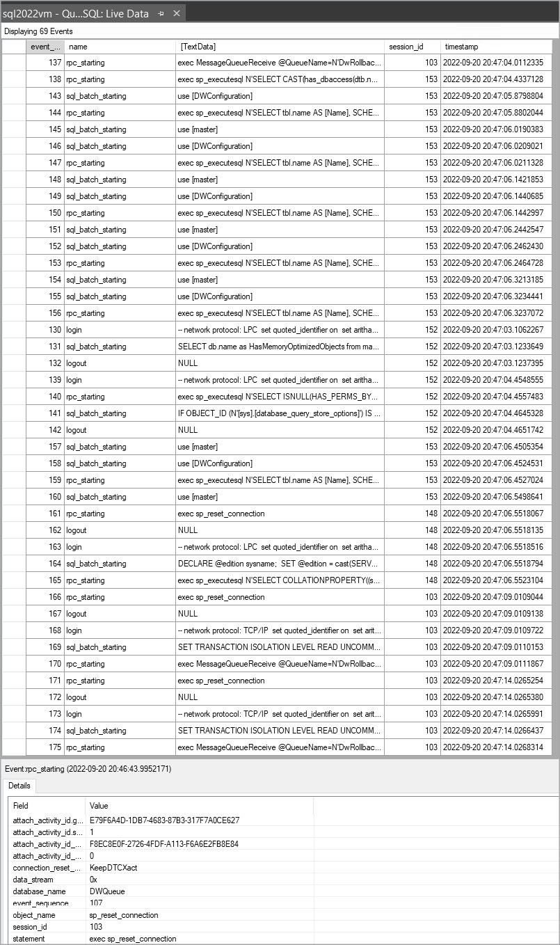
Figure 8-1 The XE Profiler T-SQL live events display in SSMS, similar to the deprecated Profiler T-SQL trace template.
Note
Though not a full replacement for SSMS, Azure Data Studio also has capabilities for managing Extended Event sessions, via the SQL Server Profiler extension that can be quickly downloaded and added. Search for the “SQL Server Profiler” extension or add the “Admin Pack for SQL Server” extension via the Extensions Marketplace in Azure Data Studio.
An Extended Events session can generate simultaneous output to multiple destinations, only one of which closely resembles the .trc files of old.
You can create other targets for a session on the Data Storage page of the New Session dialog box in SSMS. To view data collected by the target, expand the session, right-click the package, and select View Target Data in the shortcut menu. (See Figure 8-2.)
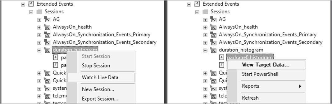
Figure 8-2 A side-by-side look at the difference between Watch Live Data on an Extended Events session and View Target Data on an Extended Events session target.
When viewing target data, you can right-click to re-sort, copy the data to the clipboard, and export most of the target data to .csv files for analysis in other software.
Unlike Watch Live Data, View Target Data does not refresh automatically. However, for some targets, you can configure SSMS to poll the target automatically by right-clicking the View Target Data window, selecting Refresh Interval in the shortcut menu, and choosing a refresh interval (between 5 seconds and 1 hour).
Note
Currently, there is no built-in way in SSMS to write Extended Events session data directly to a SQL Server table. However, the Watch Live Data interface provides easy point-and-click analysis, grouping, and filtering of live session data. We review the target types next. Take some time to explore the other available target types; they can easily and quickly reproduce your analysis of trace data written to SQL Server tables.
The section that follows presents a breakdown of the possible targets. Many of these do some of the heavy lifting that you might have done previously by writing or exporting SQL trace data to a table and then performing your own aggregations, counts, or data analysis. Remember: You don’t need to pick just one target type to collect data for your session.
Understand the variety of Extended Events targets
As mentioned, you can always watch detailed and “live” Extended Events data captured asynchronously in memory for any session through SSMS. You do this by right-clicking a session and selecting Watch Live Data from the shortcut menu. You’ll see asynchronously delivered detailed data, and you can customize the columns you see, apply filters on the data, and even create groups and on-the-fly aggregations, all by right-clicking inside the Live Data window.
The Live Data window, however, isn’t a target. The data isn’t saved anywhere outside the SSMS window, and you can’t look back at data you missed before launching Watch Live Data. You can create a session without a target, and Watch Live Data is all you’ll get, but often that is all you need for a quick observation.
Here is a summary of the Extended Event targets available to be created. Remember, you can create more than one target per session.
Event File target (.xel). Writes the event data to a physical file on a drive asynchronously. You can then open and analyze it later, much like deprecated trace files, or merge it with other .xel files to assist analysis. (In SSMS, select the File menu, select Open, and then select Merge Extended Events Files.)
If you are using Azure SQL Database or Managed Instance and you would like to persist Extended Event data, you can only use the Event File target to Azure Blob Storage. You also need to create a credential using a shared access signature (SAS).
- The instructions for connecting your Azure SQL Database and Blob Storage for Extended Events can be found at https://learn.microsoft.com/azure/azure-sql/database/xevent-code-event-file.
When you view the event file data in SSMS (right-click the event file and select View Target Data), the data does not refresh live. Data continues to be written to the file behind the scenes while the session is running. So, to view the latest data, you must close the .xel file and open it again.
By default, .xel files are written to the instancepathMSSQLLog folder.
Histogram target. Counts the number of times an event has occurred and bucketizes an action, storing the data in memory. For example, you can capture a histogram of
sql_statement_completedbroken down by the number of observed events by client-hostname action, or by the duration field.When configuring the histogram type target, you must choose a number of buckets (or slots, in the T-SQL syntax) that is greater than the number of unique values you expect for the action or field. If you’re bucketizing by a numeric value such as duration, be sure to provide a number of buckets larger than the largest duration you could capture over time. If the histogram runs out of buckets for new values for your action or field, it will not capture data for them.
You can provide any number of histogram buckets, but the histogram target will round the number up to the nearest power of 2. Thus, if you provide a value of 10 buckets, you’ll see 16 buckets.
Pair matching or Pairing target. Used to match events, such as the start and end of a SQL Server batch execution, and find occasions when an event in a pair occurs without the other, such as
sql_statement_startingandsql_statement_completed. Select a start and an end from the list of actions you’ve selected.Ring_buffer target. Provides a fast, in-memory first in, first out (FIFO) asynchronous memory buffer to collect rapidly occurring events. Stored in a memory buffer, the data is never written to a drive, allowing for robust data collection without performance overhead. The customizable dataset is provided in XML format and must be queried. Because this data is in-memory, you should be careful how high you configure the Maximum Buffer Memory size, and never set the size to 0 (unlimited).
Service Broker target. Used to send messages to a target service of a customizable message type.
Although the aforementioned targets are high-performing asynchronous targets, there are two synchronous targets:
Event Tracing for Windows (ETW) target. Used to gather SQL Server data, to be combined with Windows event log data, for troubleshooting and debugging Windows applications.
Event counter target. Counts the number of events in an Extended Events session. You use this to provide data for trending and later aggregate analysis. The resulting dataset has one row per event with a count. This data is stored in memory, so although it’s synchronous, you shouldn’t expect any noticeable performance impact.
Note
Be aware when using synchronous targets that the resource demand of synchronous targets might be more noticeable.
Further, there are two session options that can affect the performance impact of an Extended Event session. The defaults are reasonably safe and are unlikely to result in noticeable performance overhead, so they don’t typically need to be changed. You might, however, want to change them if the event you’re trying to observe is rare, temporary, and outweighs your performance overhead concerns.
EVENT_RETENTION_MODE. Determines whether, under pressure, the Extended Event session can miss a captured event. The default,
ALLOW_SINGLE_EVENT_LOSS, here can let target(s) miss a single event when memory buffers used to stream the data to the target(s) are full.You instead specify
ALLOW_MULTIPLE_EVENT_LOSS, which further minimizes the potential for performance impact on the monitored server by allowing more events to be missed.Or you could specify
NO_EVENT_LOSS, which does not allow events to be missed, even if memory buffers are full. All events are retained and presented to the target. While not the same as using a synchronous target, it can result in the same effect: Performance of the SQL Server could suffer under the weight of the Extended Event session. Using this option is not recommended.MAX_DISPATCH_LATENCY. Determines the upper limit for when events are sent from the memory buffer to the target. By default, events are buffered in memory for up to 30 seconds before being sent to the targets. You could change this value to
1to force data out of memory buffers faster, reducing the benefit of the memory buffers. A value ofINFINITEor0allows for the retention of events until memory buffers are full or until the session closes.
Let’s look at querying Extended Events session data in T-SQL with a couple of practical common examples.
Use Extended Events to capture deadlocks
We’ve talked about viewing data in SSMS, so let’s review querying Extended Events data via T-SQL. Let’s query one of the default Extended Events sessions, system_health, for deadlocks.
Back before SQL Server 2008, it was not possible to see a deadlock. You had to see it coming—to enable one or more trace flags before the deadlock, which allowed deadlocks to be captured to the SQL Server Error Log. With the system_health Extended Events session, a recent history of event data is captured, included deadlock graphs. This data is captured to both a ring_buffer target with a rolling 4-MB buffer, and to an .xel file with a total of 20 MB in rollover files. Either target will contain the most recent occurrences of the xml_deadlock_report event, and although the ring_buffer is faster to read from, the .xel file by default contains more history. Further, the .xel file isn’t subject to the limitations of the 4-MB ring_buffer target or the potential for missed rows.
The T-SQL code sample that follows demonstrates the retrieval of the .xel file target as XML:
DECLARE @XELFile nvarchar(256), @XELFiles nvarchar(256)
           , @XELPath nvarchar(256);
--Get the folder path where the system_health .xel files are
SELECT     @XELFile =       CAST(t.target_data as XML)
          .value('EventFileTarget[1]/File[1]/@name', 'NVARCHAR(256)')
FROM sys.dm_xe_session_targets t
     INNER JOIN sys.dm_xe_sessions s
      ON s.address = t.event_session_address
WHERE s.name = 'system_health' AND t.target_name = 'event_file';
--Provide wildcard path search for all currently retained .xel files
SELECT @XELPath =
    LEFT(@XELFile, Len(@XELFile)-CHARINDEX('',REVERSE(@XELFile)))
SELECT @XELFiles = @XELPath + 'system_health_*.xel';
--Query the .xel files for deadlock reports
SELECT DeadlockGraph = CAST(event_data AS XML)
     , DeadlockID = Row_Number() OVER(ORDER BY file_name, file_offset)
FROM sys.fn_xe_file_target_read_file(@XELFiles, null, null, null) AS F
WHERE event_data like '<event name="xml_deadlock_report%';This example returns one row per captured xml_deadlock_report event and includes an XML document, which in SSMS Grid results will appear as a blue hyperlink. Select the hyperlink to open the XML document, which will contain complete details of all elements of the deadlock. If you want to see a deadlock graph, save this file as an .xdl file, and then open it in SSMS.
Use Extended Events to detect autogrowth events
The SQL Server default trace captures historical database data and log file autogrowth events, but the default Extended Events sessions shipped with SQL Server do not. The Extended Events that capture autogrowth events are database_file_size_change and databases_log_file_size_changed. Both events capture autogrowths and manual file growths run by ALTER DATABASE … MODIFY FILE statements, and include an event field called is_automatic to differentiate them. Additionally, you can identify the query statement sql_text that prompted the autogrowth event.
The following is a sample T-SQL script to create a startup session that captures autogrowth events to an .xel event file (which is written to F:Data—you should change this to an appropriate directory on your system) and also a histogram target that counts the number of autogrowth instances per database:
CREATE EVENT SESSION [autogrowths] ON SERVER
ADD EVENT sqlserver.database_file_size_change(
 ACTION(package0.collect_system_time,sqlserver.database_id
,sqlserver.database_name,sqlserver.sql_text)),
ADD EVENT sqlserver.databases_log_file_size_changed(
 ACTION(package0.collect_system_time,sqlserver.database_id
,sqlserver.database_name,sqlserver.sql_text))
ADD TARGET package0.event_file(
--.xel file target
SET filename=N'F:DATAautogrowths.xel'),
ADD TARGET package0.histogram(
--Histogram target, counting events per database_name
SET filtering_event_name=N'sqlserver.database_file_size_change'
,source=N'database_name',source_type=(0))
--Start session at server startup
WITH (STARTUP_STATE=ON);
GO
--Start the session now
ALTER EVENT SESSION [autogrowths]
ON SERVER STATE = START;- Refer to the section “Understand and find autogrowth events” earlier in this chapter for more information, including how to prevent autogrowth events.
Use Extended Events to detect page splits
As discussed, detecting page splits can be useful. You might choose to monitor page splits when load testing a table design with its intended workload, or when finding insert statements that cause the most fragmentation.
The following sample T-SQL script creates a startup session that captures autogrowth events to an .xel event file, and also a histogram target that counts the number of page splits per database:
CREATE EVENT SESSION [page_splits] ON SERVER
ADD EVENT sqlserver.page_split(
 ACTION(sqlserver.database_name,sqlserver.sql_text))
ADD TARGET package0.event_file(
SET filename=N'page_splits', max_file_size=(100)),
ADD TARGET package0.histogram(
SET filtering_event_name=N'sqlserver.page_split'
,source=N'database_id',source_type=(0))
--Start session at server startup
WITH (STARTUP_STATE=ON);
GO
--Start the session now
ALTER EVENT SESSION [page_splits] ON SERVER STATE = START;- Refer to the section “Track page splits” earlier in this chapter for more information, including how to prevent page splits.
Secure Extended Events
You can also think of Extended Events as a diagnostic tool for developers. Given knowledge of your own data classification and regulatory requirements, you should consider granting the necessary permissions to developers, even if temporarily.
There are certain sensitive events that you cannot capture with a trace or Extended Event session. For example, the T-SQL statement CREATE LOGIN for a SQL-authenticated login will not capture the value of the password.
To access Extended Events in SQL Server, a developer needs the ALTER ANY EVENT SESSION permission. This grants that person access to create Extended Events sessions by using T-SQL commands, but not to view server metadata in the New Extended Events Session Wizard in SSMS. For that, you need one further commonly granted developer permission: VIEW SERVER STATE.
In Azure SQL Database, Extended Events have the same capability, but for developers to view Extended Events sessions, you must grant them an ownership-level permission, CONTROL DATABASE. However, we do not recommend this for developers or non-administrators in production environments.
- For more about object permissions, see Chapter 12, “Administer instance and database security and permissions.”
Capture performance metrics with DMOs and data collectors
For years, server administrators have used the Windows Performance Monitor (perfmon.exe) application to visually track and collect performance information about server resources, application memory usage, disk response times, and so on. In addition to the live Performance Monitor graph, you can also configure Data Collector Sets in Performance Monitor to gather the same metrics over time.
SQL Server has many metrics made visible through DMVs as well. This book has neither the scope nor the space to investigate and explain every available performance metric, or even every useful one. Instead, this section reviews the tools and covers a sampling of important performance metrics.
These metrics exist at the OS or instance level, so this chapter does not review granular data for individual databases, workloads, or queries. However, identifying performance with isolated workloads in near-production systems is possible. Like aggregate wait statistics, there is significant value in trending these Performance Monitor metrics on server workloads, monitoring peak behavior metrics, and for immediate troubleshooting and problem diagnosis.
Query performance metrics with DMVs
Beyond the Windows Performance Monitor and Linux metrics, this chapter has already mentioned a DMV that exposes most of the performance metrics within SQL Server: sys.dm_os_performance_counters. It behaves the same in Windows and Linux, thanks to the magic of the SQL Platform Abstraction Layer (SQLPAL), which helps SQL Server look and act much the same way on both Windows and Linux.
There are some advantages to this DMV in that you can combine it with other DMVs that report on system resource activity (check out sys.dm_os_sys_info, for example), and you can fine-tune the query for ease of monitoring and custom data collecting. However, sys.dm_os_ performance_counters does not currently have access to metrics outside the SQL Server instance categories—even the most basic operating system metrics, like % Processor Time.
The following code sample uses sys.dm_os_performance_counters to return the operating system’s total memory, the instance’s current target server memory, total server memory, and page life expectancy:
SELECT Time_Observed = SYSDATETIMEOFFSET()
, OS_Memory_GB = MAX(convert(decimal(19,3), os.physical_memory_kb/1024./1024.))
, OS_Available_Memory_GB = max(convert(decimal(19,3),
sm.available_physical_memory_kb/1024./1024.))
, SQL_Target_Server_Mem_GB = max(CASE counter_name
WHEN 'Target Server Memory (KB)' THEN convert(decimal(19,3), cntr_value/1024./1024.)
END)
, SQL_Total_Server_Mem_GB = max(CASE counter_name
WHEN 'Total Server Memory (KB)' THEN convert(decimal(19,3), cntr_value/1024./1024.)
END)
, PLE_s = MAX(CASE counter_name WHEN 'Page life expectancy' THEN cntr_value END)
FROM sys.dm_os_performance_counters as pc
CROSS JOIN sys.dm_os_sys_info as os
CROSS JOIN sys.dm_os_sys_memory as sm;
Note
In servers with multiple SQL Server instances, sys.dm_os_performance_counters displays only metrics for the instance on which it is run. You cannot access performance metrics for other instances on the same server via this DMV.
Some queries against sys.dm_os_performance_counters are not as straightforward. For example, although Performance Monitor returns the Buffer Cache Hit Ratio as a single value, querying this same memory metric via the DMV requires creating the ratio from two metrics. This code sample divides two metrics to provide the Buffer Cache Hit Ratio:
SELECT Time_Observed = SYSDATETIMEOFFSET(),
Buffer_Cache_Hit_Ratio = convertDECIMAL (9,1)t, 100 *
(SELECT cntr_value = convert(decimal (9,1), cntr_value)
FROM sys.dm_os_performance_counters as pc
WHERE pc.COUNTER_NAME = 'Buffer cache hit ratio'
AND pc.OBJECT_NAME like '%:Buffer Manager%')
/
(SELECT cntr_value = convert(decimal (9,1), cntr_value)
FROM sys.dm_os_performance_counters as pc
WHERE pc.COUNTER_NAME = 'Buffer cache hit ratio base'
AND pc.OBJECT_NAME like '%:Buffer Manager%'));
Finally, some counters returned by sys.dm_os_performance_counters are continually incrementing integers. Let’s return to our earlier example of finding page splits, where we demonstrated how to find the accumulating value. The counter name Page Splits/sec is misleading when accessed via the DMV, because it is an incrementing number. To calculate the rate of page splits per second, you need two samples to calculate the difference between the first and second values. This strategy is appropriate only for single-value counters for the entire server or instance. For counters that return one value per database, you would need to use a temporary table to calculate the rate for each database between the two samples. You could also capture these values to a table at regular intervals to enable reporting over time.
DECLARE @page_splits_Start_ms bigint, @page_splits_Start bigint
, @page_splits_End_ms bigint, @page_splits_End bigint;
SELECT @page_splits_Start_ms = ms_ticks
, @page_splits_Start = cntr_value
FROM sys.dm_os_sys_info CROSS APPLY
sys.dm_os_performance_counters
WHERE counter_name ='Page Splits/sec'
AND object_name LIKE '%SQL%Access Methods%'; --Find the object that contains page splits
WAITFOR DELAY '00:00:05'; --Duration between samples 5s

SELECT @page_splits_End_ms = MAX(ms_ticks),
@page_splits_End = MAX(cntr_value)
FROM sys.dm_os_sys_info CROSS APPLY
sys.dm_os_performance_counters
WHERE counter_name ='Page Splits/sec'
AND object_name LIKE '%SQL%Access Methods%'; --Find the object that contains page splits
SELECT Time_Observed = SYSDATETIMEOFFSET(),
Page_Splits_per_s = convert(decimal(19,3),
(@page_splits_End - @page_splits_Start)*1.
/ NULLIF(@page_splits_End_ms - @page_splits_Start_ms,0));
You can gain access to some OS metrics via the DMV sys.dm_os_ring_buffers, including metrics on CPU utilization and memory. This DMV returns thousands of XML documents, generated every second, loaded with information on SQL exceptions, memory, schedulers, connectivity, and more. It is worth noting that the sys.dm_os_ring_buffers DMV is one of several OS-level views that are documented but not supported.
- For more information, visit https://learn.microsoft.com/sql/relational-databases/system-dynamic-management-views/sql-server-operating-system-related-dynamic-management-views-transact-sql.
In the code sample that follows, we pull the SQL Server instance’s CPU utilization and the server idle CPU percentage for the past few hours. The remaining CPU percentage can be chalked up to other applications or services running on the server, including other SQL Server instances.
DECLARE @ts_now bigint = (SELECT cpu_ticks/(cpu_ticks/ms_ticks) FROM sys.dm_os_sys_info
WITH (NOLOCK));

SELECT TOP(256) SQLProcessUtilization AS [SQL Server Process CPU Utilization],
SystemIdle AS [System Idle Process],
100 - SystemIdle - SQLProcessUtilization AS [Other Process CPU Utilization],
DATEADD(ms, -1 * (@ts_now - [timestamp]), GETDATE()) AS [Event Time]
FROM (SELECT record.value('(./Record/@id)[1]', 'int') AS record_id,
record.value('(./Record/SchedulerMonitorEvent/SystemHealth/SystemIdle)[1]', 'int')
AS [SystemIdle],
record.value('(./Record/SchedulerMonitorEvent/SystemHealth/ProcessUtilization)[1]',
'int')
AS [SQLProcessUtilization], [timestamp]
FROM (SELECT [timestamp], CONVERT(xml, record) AS [record]
FROM sys.dm_os_ring_buffers WITH (NOLOCK)
WHERE ring_buffer_type = N'RING_BUFFER_SCHEDULER_MONITOR'
AND record LIKE N'%<SystemHealth>%') AS x) AS y
ORDER BY record_id DESC;
Now you should have a grasp on using most of the DMVs for gathering performance metrics to capture various types of data streams coming out of SQL Server.
- For more information on using trace flags to disable ring-buffer data collection, visit https://support.microsoft.com/help/920093.
Capture performance metrics with Performance Monitor
To get a complete, graphical picture of server resource utilization, it’s necessary to use a server resource tool. Performance Monitor is more than just a pretty graph; it is a suite of data collection tools that can persist outside your user profile.
To open Performance Monitor, type performance in the Windows Start menu and select the Performance Monitor icon, or press the Windows+R key combination and type perfmon. You can configure the live Performance Monitor graph, available in the Monitoring Tools folder, to show a live picture of server performance. To do so, right-click the (mostly empty) chart to access properties, add counters, clear the graph, and so on.
Choosing Properties in that same shortcut menu opens the Performance Monitor Properties dialog box. Under General, you can configure the sample rate and duration of the graph. You can also display up to 1,000 sample points on the graph live. This can be 1,000 1-second sample points for a total of 16 minutes and 40 seconds, or more time if you continue to decrease the sample frequency. For example, you can display 5,000 5-second sample points, for more than 83 minutes of duration in the graph.
A Data Collector Set allows you to collect data from one or more Performance Monitor counters, and to run that collection non-interactively. This data is stored in log files and is how administrators most commonly use Performance Monitor. You can access the collected Performance Monitor data by navigating to the Reports folder; the User Defined folder contains a new report with the graph created by the Data Collector. Figure 8-3 shows that more than 15 days of data performance was collected in the Data Collector, which we’re viewing in the Memory folder, selecting the most recent report that was generated when we stopped the Memory Data Collector Set.
Figure 8-3 The Windows Performance Monitor application.
Monitor key performance metrics
This section contains some Performance Monitor metrics to look at when assessing the health and performance of your SQL Server. Although we don’t have the space in this book to provide a deep dive into each metric, its causes, and its indicators, you should take time to investigate and research metrics on your server that appear outside with the guidelines provided here.
We don’t provide many hard numbers in this section—things like “Metric X should always be lower than Y.” You should track trends, measure metrics at peak activity, and investigate how metrics respond to server, query, and configuration changes. What might be normal for an instance with a read-heavy workload might be problematic for an instance with a high-volume write workload, and vice versa.
The following subsections review common performance monitoring metrics, including where to find them in Windows Performance Monitor and in SQL Server DMOs if available. When one of these sections contains a DMV entry, it means the corresponding metric is available in Windows and Linux. When not available via DMVs, you can find these same OS-level metrics in Linux using tools detailed in the next section, “Monitor key performance metrics in Linux.”
Average Disk seconds per Read or Write
Performance Monitor: PhysicalDisk:Avg. Disk sec/Read and PhysicalDisk:Avg. Disk sec/Write
DMO: sys.dm_io_virtual_file_stats offers similar metrics for each data and log file. Typically, this data is used in conjunction with the Performance Monitor data to confirm or deny behavior.
View this metric on each volume. The _Total metric doesn’t have any value here; you should look at individual volumes in which SQL Server files are present. This metric has the clearest guidance of any with respect to what is acceptable or not for a server.
Try to measure this value during your busiest workload, and also during backups. You want to see the average disk seconds per read and write operation (considering that a single query could have thousands or millions of operations) below 20 milliseconds, or .02 seconds. Below 10 milliseconds is optimal and very achievable with modern storage systems.
- This is the rare case for which we have hard and fast numbers specified by Microsoft to rely on. For more information, visit the “Monitoring Disk Usage” blog post at https://social.technet.microsoft.com/wiki/contents/articles/3214.monitoring-disk-usage.aspx.
Seeing this value spike to a very high value (such as .1 second or 100 milliseconds) isn’t a major cause for concern, but if you see these metrics sustaining an average higher than .02 seconds during peak activity, it is a fairly clear indication that the physical I/O subsystem is being stressed beyond its capacity. Low, healthy measurements for this number don’t provide any insight into the quality or efficiency of queries and execution plans, only the response from the disk subsystem. The Avg. Disk sec/Transfer counter is simply a combination of both read and write activity, unrelated to Avg. Disk Transfers/sec.
Page Life Expectancy (PLE)
Performance Monitor: MSSQL$InstanceName:Buffer Manager/Page Life Expectancy (s)
DMV: sys.dm_os_performance_counters
WHERE object_name like '%Buffer Manager%'
AND counter_name = 'Page life expectancy'
Page Life Expectancy (PLE) is a measure of time (in seconds) that indicates the age of data in memory. PLE is one of the most direct indicators of memory pressure, though it doesn’t provide a complete picture of memory utilization in SQL Server. In general, you want pages of data in memory to grow to a ripe old age; when they do, it means there is ample memory available to SQL Server to store data to serve reads without going back to the storage layer.
A dated, oft-quoted metric of 300 seconds isn’t applicable to many SQL Server instances. While 300 seconds might be appropriate for a server with 4 GB of memory, it’s far too low for a server with 64 GB of memory. Instead, you should monitor this value over time. Does PLE bottom out and stay there during certain operations or scheduled tasks? If so, your SQL Server performance might benefit from more memory during those operations. Does PLE grow steadily throughout production hours? If so, the data in memory is likely to be sufficient for the observed workload.
Page Reads
Performance Monitor: MSSQL$InstanceName:Buffer Manager/Page reads/sec
DMV: sys.dm_os_performance_counters
WHERE object_name like '%Buffer Manager%'
AND counter_name = 'Page reads/sec'
This is an average of the number of page read operations completed recently. The title is a bit misleading—these aren’t page reads out of the buffer; rather, they are out of physical pages on the drive, which is slower than data pages coming out of memory.
You should make the effort to lower this number by optimizing queries and indexing, improving efficiency of cache storage, and, of course, as a last resort, increasing the amount of server memory. Although every workload is different, a value less than 90 is a broad, overly simple guideline. High numbers indicate inefficient query and index design in read-write workloads or memory constraints in read-heavy workloads.
Memory Pages
Performance Monitor: Memory:Pages/sec
DMV: Not available.
Similar to Buffer ManagerPage Reads/sec, this is a way to measure data coming from a drive as opposed to coming out of memory. This metric is a recent average of the number of pages pulled from a drive into memory, which will be high after SQL Server startup. Although every workload is different, a value of less than 50 is a broad guideline. Sustained high or climbing levels during typical production usage indicate inefficient query and index design in read-write workloads, or memory constraints in read-heavy workloads. Spikes during database backup and restore operations, bulk copies, and data extracts are expected.
Batch Requests
Performance Monitor: MSSQL$lnstanceName:SQL StatisticsBatch Requests/sec
DMV: sys.dm_os_performance_counters WHERE object_name like '%SQL Statistics%' AND counter_name = 'Batch Requests/sec'
This is a measure of aggregate SQL Server user activity, indicating the recent average of the number of batch requests. Any command issued to the SQL Server contains at least one batch request. Higher sustained numbers are good; they mean your SQL Server instance is sustaining more traffic. Should this number trend downward during peak business hours, it means your SQL Server instance is being outstripped by increasing user activity.
Page Faults
Performance Monitor: MemoryPage Faults/sec
DMV: Not available.
A memory page fault occurs when an application seeks a data page in memory, only to find it isn’t there because of memory churn. A soft page fault indicates the page was moved or otherwise unavailable; a hard page fault indicates the data page was not in memory and must be retrieved from the drive. The Page Faults/sec metric captures both.
Page faults are a symptom, the cause being memory churn, so you might see an accompanying drop in Page Life Expectancy (PLE). Spikes in page faults, or an upward trend, indicate the amount of server memory was insufficient to serve requests from all applications, not just SQL Server.
Available Memory
Performance Monitor: MemoryAvailable Bytes or MemoryAvailable KBytes or MemoryAvailable MBytes
DMV: SELECT available_physical_memory_kb FROM sys.dm_os_sys_memory
Available memory is operating system memory currently unallocated to any application. Server memory above and beyond the SQL Server instance(s) total MAX_SERVER_MEMORY setting, minus memory in use by other SQL Server features and services or other applications, is available. This will roughly match what shows as available memory in the Windows Task Manager.
Total Server Memory
Performance Monitor: MSSQL$InstanceName:Memory ManagerTotal Server Memory (KB)
DMV: sys.dm_os_performance_counters
WHERE object_name like '%Memory Manager%'
AND counter_name = 'Total Server Memory (KB)'
This is the actual amount of memory that SQL Server is using. It is often contrasted with the next metric (Target Server Memory). This number might be far larger than what Windows Task Manager shows allocated to the SQL Server Windows NT 64 Bit background application, which shows only a portion of the memory that sqlserver.exe controls. The Total Server Memory metric is correct.
Target Server Memory
Performance Monitor: MSSQL$InstanceName:Memory ManagerTarget Server Memory (KB)
DMV: sys.dm_os_performance_counters
WHERE object_name like '%Memory Manager%'
AND counter_name = 'Target Server Memory (KB)'
This is the amount of memory to which SQL Server wants to have access and is currently working toward consuming. If the difference between Target Server Memory and Total Server Memory is larger than the value for Available Memory, SQL Server wants more memory than the Windows Server can currently acquire. SQL Server will eventually consume all memory available to it under the Max Server Memory setting, but it might take time.
Monitor key performance metrics in Linux
While monitoring SQL Server on Linux is identical to SQL Server on Windows in most ways, there are some exceptions, especially when the monitoring source is coming from outside the SQLPAL.
As stated, you’ll find that the DMOs perform the same for SQL Server instances on Windows and in Linux. It’s in the OS layer that the differences in metrics available, and especially the tools used to collect them, are stark. This section reviews a sampling of tools you can use for Linux-specific OS monitoring, keeping in mind that there is a wealth of monitoring solutions on various Linux distributions.
- For more about SQL Server on Linux, see Chapter 5, “Install and configure SQL Server on Linux.”
View performance counters in Linux
The dynamic management view sys.dm_os_performance_counters behaves the same and delivers identical output on Windows and Linux. For example, the Performance Monitor metrics in the previous section listed as available in the DMV are also available in SQL Server on Linux.
The top command, built into Linux and with near-identical output on all distributions, launches a live full-console display of CPU and memory utilization and process metrics, not dissimilar from Windows Task Manager. The screen is data rich and starkly black and white, however, so consider the more graphical command htop. Though not present by default on all Linux distributions, it can be quickly downloaded and easily installed. This command’s output (see Figure 8-4) shows much of the same useful data with a more pleasant format and with color highlights.
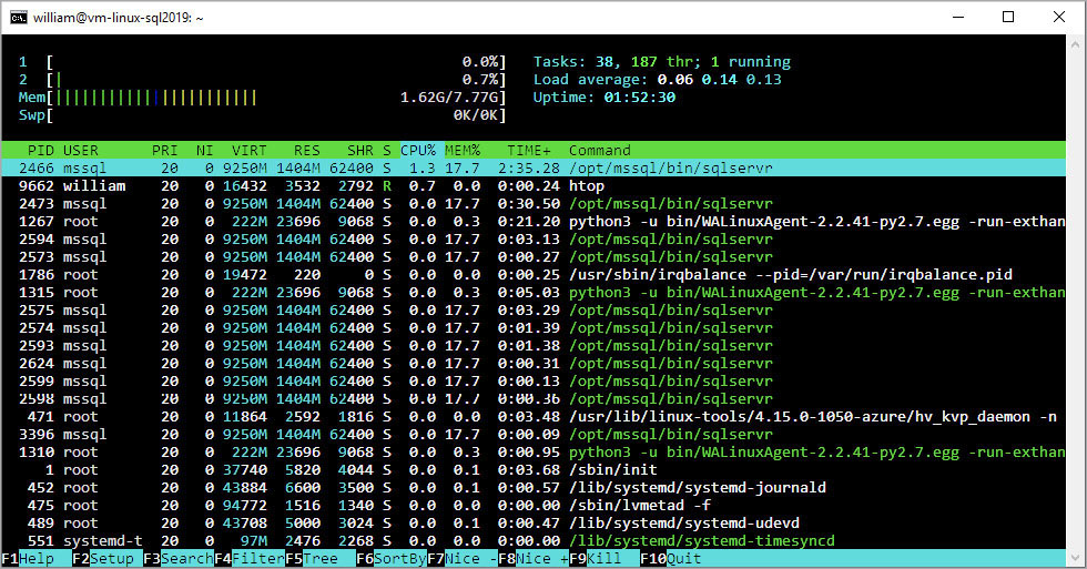
Figure 8-4 The htop command’s live, updating look at the Linux server’s CPU, memory, and process utilization.
Another built-in Linux tool is vmstat, which includes extended information on process memory, like runnable/sleeping processes, memory availability, swap memory use, memory I/O activity, system interrupts, and CPU utilization percentages. While vmstat returns a snapshot of the data, the syntax vmstat n appends fresh data to the console once every n seconds.
For querying items in SQL Server on Linux not available in sys.dm_os_performance_counters, such as Avg Disk sec/read and Avg Disk sec/write for each volume, different Linux tools are needed.
The iostat tool is available to install via the syststat performance monitoring tools, using the package manager on your operating system. Source code for iostat is available at https://github.com/sysstat/sysstat.
For example:
user@instance:~$ iostat -xUsing the -x parameter to return extended statistics yields basic host information, a current CPU activity utilization breakdown, and a variety of live measurements for devices, including logical disk volumes. The measures r_await and w_await are the average durations in milliseconds for read and write requests.
Other alternative packages include dtrace and nmon, the latter of which includes a simple bash-based GUI.
Monitor key performance metrics in Azure portal
The Azure portal provides a significant amount of intelligence to cloud-based SQL operations with built-in dashboarding. This section doesn’t delve too deeply into those continuously improving standard features, but it does spend a little time talking about the sophisticated custom dashboarding and monitoring via Kusto and Azure Log Analytics.
View data in Azure Monitor
The Azure platform’s built-in metrics tool, Azure Monitor—accessible via the Azure portal—automatically tracks several basic key performance and usage metrics in any Azure SQL Database. Azure Monitor Logs is one half of the data platform that supports Azure Monitor. The other is Azure Monitor Metrics, which stores numeric data in a time-series database. Some of these metrics are configured for you as part of the service (like metrics) while others require you to configure them (for example, SQL Diagnostics).
You query this data via the Azure Monitor Metrics pane, where you can drill down to an Azure resource and choose a metric to generate visualizations. Azure Monitor supports pinning generated visualizations to Azure portal dashboards, allowing you to create and monitor key database metrics at a glance.
When using Azure Monitor Metrics for an Azure SQL Database, for example, you can add metrics for DTU usage, or for percentages of the measures that make up a DTU. In the example in Figure 8-5, the Azure Monitor Metrics pane displays both DTU used and the average Log IO percentage on the same graph.
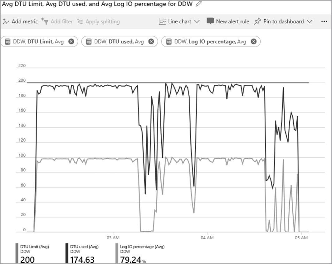
Figure 8-5 The Azure Monitor Metrics pane for an Azure SQL Database.
You can do more complicated charting via Azure Monitor by adding more metrics, which allows for visualization of multiple dimensions of interrelated data simultaneously, such as service request count per hour versus database CPU or DTU utilization.
You use filtering or splitting to further break down metrics with more than one value—for example, disk metrics. You can either filter on specific LUNs when viewing Data Disk Read Bytes/sec, for example, or you can split the data into different graph series, one for each LUN. If this sounds familiar, filtering and splitting using the Azure portal is not dissimilar from the same in Windows Performance Monitor. For example, this is similar to the selection of volumes when adding the Physical DiskAvg. Disk sec/Read counter.
Leverage Azure Monitor logs
Azure Monitor is built on the Azure Log Analytics platform, using the same data storage and query mechanisms. Azure Log Analytics is itself a separate platform built to aggregate and query big data of varying schemas in near-real time. Azure Monitor log data is stored in a Log Analytics workspace, but is distinctly under the Azure Monitor product name, which also includes Application Insights.
Many Microsoft Azure resource types natively support syncing varying diagnostic and metric information to Azure Log Analytics. Azure SQL Database natively supports the export of information to Log Analytics via the Diagnostic Settings pane for the respective database in the Azure portal. Diagnostic settings support streaming basic metrics, as well as varying types of logs to log analytics.
Contrary to Azure Monitor, Log Analytics supports the ingesting of information from on-premises servers as well via the Azure Log Analytics agent. You might be familiar with the System Center Operations Manager (SCOM) monitoring tool, the Microsoft Monitoring Agent (MMA). The Azure Monitor agent is the evolution and replacement of the MMA and enables you to attach to an Azure Monitor or send data to a Log Analytics workspace.
Once your Log Analytics workspace is receiving data, you can query the workspace via the Logs pane in the Log Analytics workspace resource using the Kusto Query Language (KQL).
The following sample query gathers all DTU consumption metrics for Azure SQL Databases sending their logs to the Log Analytics workspace. It displays the 80th percentile of DTU consumption per time grain—in this case every 60 minutes. The intent is to normalize spikes of DTU usage and help to visualize sustained increase in DTU percentage that may be indicative of inefficient queries or a degradation between deployments.
AzureMetrics
| where MetricName == 'dtu_consumption_percent'
| summarize percentile(Average, 80) by bin(TimeGenerated, 1h)
| render timechart- For more on KQL, see https://learn.microsoft.com/azure/data-explorer/kusto/query/.
Figure 8-6 visualizes the results of this query, which will work with any Log Analytics workspaces that have SQL databases sending log data.
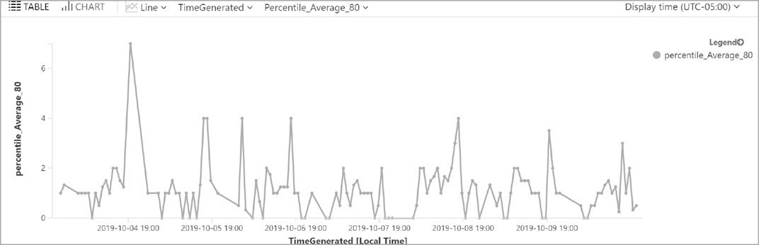
Figure 8-6 A Log Analytics query using Kusto and its charted result of average DTU utilization over time.
Note
As with Azure Monitor, results of Log Analytics queries can be pinned to a Microsoft Azure portal dashboard by using the Pin to Dashboard button in the header bar.
As mentioned, the preceding query extrapolates the 80th percentile of average DTU usage as a percent of quota, denoted by 'dtu_consumption_percent', in 1-hour increments. While useful, variances in usage patterns of the databases can lead to numerous peaks and valleys in the data rendered. This can make it hard to visually spot when the analyzed data is indicating a regression in performance—that is, a spike in DTU consumption.
As an alternative, the following query, visualized in Figure 8-7, applies a finite impulse response (series_fir()) to produce a 12-hour moving average of the analyzed data. This type of function is often used in signal processing, which a log stream resembles. This second example is a minor demonstration of the power and ease of drawing meaningful metrics out of the log data stream coming from Azure SQL resources, a more sophisticated look that should be more useful and readable at larger time scales.
AzureMetrics
| where MetricName == 'dtu_consumption_percent'
| make-series 80thPercentile=percentile(Average, 80)
 on TimeGenerated in range(ago(7d), now(), 60m)
| extend 80thPercentile=series_fir(80thPercentile, repeat(1, 12), true, true)
| mv-expand 80thPercentile, TimeGenerated
| project todouble(80thPercentile), todatetime(TimeGenerated)
| render timechart with (xcolumn=TimeGenerated)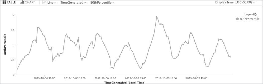
Figure 8-7 A Log Analytics query graph shows the output of a Kusto Query Language query.
- For more on
series_fir(), see https://learn.microsoft.com/azure/data-explorer/kusto/query/series-firfunction.
Create Microsoft Log Analytics solutions
Perhaps the most important takeaway from Log Analytics is the ability to add or create solution packages. These can encapsulate queries, dashboards, and drill down reports of information.
Added via the Azure Marketplace, the Azure SQL Analytics solution and SQL Health Check solution attach to a Log Analytics workspace and can provide near-immediate feedback across your environment, scaling to the hundreds of thousands of databases if necessary.
Figure 8-8 is a sample live display from a production Azure SQL Analytics solution backed by a Log Analytics workspace. It shows at-a-glance information from production Azure SQL databases regarding database tuning recommendations, resource utilization, wait types and duration, as well as health check outcomes for metrics like timeouts and deadlocks.
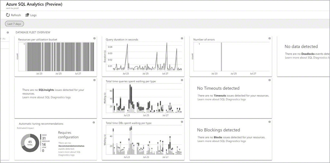
Figure 8-8 Output from the Azure SQL Analytics solution available from the Microsoft Azure Marketplace.
Protect important workloads with Resource Governor
Resource Governor, an Enterprise edition feature, is the only feature you can use to identify connections as they connect, and to limit the resources they can consume.
You can identify connections from virtually any connection property—basically, anything you can get from a system function, including the login name (SUSER_SNAME() or ORIGINAL_LOGIN()), hostname (HOST_NAME()), application name (APP_NAME()), and time functions (SYSDATETIME()).
- You can learn more about building a classifier function at https://learn.microsoft.com/sql/relational-databases/resource-governor/resource-governor-classifier-function.
After you’ve identified and classified the connection properties, you can limit properties at the individual session level or limit the resources of a resource pool. You can override the MAXDOP setting for these sessions, lower their priority, or cap the CPU, memory, or drive I/O that individual sessions can consume.
For example, you can limit all read-heavy queries coming from an SSRS server, or long-running reports coming from a third-party reporting application, or dashboard/search queries based on their application name or login. Then, you can limit these queries as a set, capping them to 25 percent of the process, disk I/O, or SQL Server memory. SQL Server will enforce these limitations and potentially slow down the identified queries; meanwhile, important read-write workloads continue to operate with the remaining 75 percent of the server’s resources.
Be aware that using Resource Governor to limit long-running SELECT statements, for example, does not alleviate concurrency issues caused by locking. In fact, limiting long-running queries could alleviate memory or CPU contention but exacerbate existing locking problems.
- See Chapter 14 for strategies to overcome concurrency issues, keeping in mind that using the
READ UNCOMMITTEDisolation level is a risky, clumsy strategy to solving concurrency issues in your applications.
When enabled, Resource Governor is transparent to connecting applications. No code changes are required in the queries to implement Resource Governor, only a working knowledge of the connection properties you will use to identify queries, such as those returned by APP_NAME(), HOST_NAME(), or SUSER_SNAME().
Caution
The value returned by APP_NAME(), or that appears in the sys.dm_exec_sessions.program_name column, is specified in the application connection string. Filtering by this value should not be used as a security method, as connection strings can be changed to specify any string. If you’re a paranoid DBA, it may also be something to watch for, if savvy users or tricky developers realize they can change their application connection strings and get more resources for their queries!
By default, sessions are split between two workload groups: workload group 1, named internal for system queries internal to the Database Engine, and workload group 2, named default for all other user queries. You can find the current groups in the DMV sys.resource_governor_workload_groups. While these groups still appear in SQL Server editions other than Enterprise (or Developer or Evaluation), Resource Governor is an Enterprise-only feature.
Configure the Resource Governor classifier function
Before configuring Resource Governor to classify workloads arriving at your SQL Server, you must create a classifier function in the master database that operates at the creation of every new session. You can write the classifier function however you like, but keep in mind that it will be run for each new connection, so it should be as efficient and simple as possible.
The classifier function must return a sysname data type value. (The sysname built-in user-defined data type is equivalent to nvarchar(128) NOT NULL.) The classifier function return value must be the name of a Resource Governor workload group to which a new connection is to be assigned. Though sysname defaults to a NOT NULL data type, the function can return a NULL value, meaning that the session is assigned to the default group.
A workload group is simply a container of sessions. Remember, when configuring Resource Governor defensively (as is most common), it is the default workload group that you want to protect; it contains “all other” sessions, including high–business value connections that perform application-critical functions, writes, and so on.
The sample code that follows defines a classifier function that returns GovGroupReports for all queries coming from two known-fictional reporting servers. You can see in the comments other sample connection identifying functions, with many more options possible.
CREATE FUNCTION dbo.fnCLASSIFIER() RETURNS sysname
WITH SCHEMABINDING AS
BEGIN
-- Note that any request that you do not assign a @grp_name value for returns NULL,
-- and is classified into the 'default' group.
DECLARE @grp_name sysname
IF (
--Use built-in functions for connection string properties
 HOST_NAME() IN ('reportserver1','reportserver2')
--OR APP_NAME() IN ('some application') --further samples you can use
--AND SUSER_SNAME() IN ('whateveruser') --further samples you can use
)
 BEGIN
     SET @grp_name = 'GovGroupReports';
    END
RETURN @grp_name
END;
Be mindful when querying other user resources, such as tables in a user database; this can cause a noticeable delay in connection creation. If you must have the classifier function query a table, store the table in the master database, and keep the table small and the query efficient.
After creating the function, which can have any name, you must register it as the classifier function for this instance’s Resource Governor feature. The function is still not active yet for new logins; you must set up workload groups and resource pools first, then enable your changes.
Configure Resource Governor resource pools and workload groups
Configuring resource pools (limitations that many sessions share) and workload groups (limitations for individual sessions) is the next step. You should take an iterative, gradual approach to configuring the Resource Governor, and avoid making large changes or large initial limitations to the affected groups.
If you have a preproduction environment to test the impact of Resource Governor on workloads with realistic production scale, you should consider performance load testing to make sure the chosen settings will not cause application issues due to throttling resources.
The sample code that follows can be an instructional template to creating an initial pool and group. If you seek to divide your sessions up further, multiple groups can belong to the same pool, and multiple pools can be limited differently. Commented-out examples of other common uses for Resource Governor are included. In this example, we create a pool that limits all covered sessions to 50 percent of the instance’s memory, and a group that limits any single query to 30 percent of the instance’s memory, and forces the sessions into MAXDOP = 1, overriding any server, database, or query-level setting:
CREATE RESOURCE POOL GovPoolMAXDOP1;
CREATE WORKLOAD GROUP GovGroupReports;
GO
ALTER RESOURCE POOL GovPoolMAXDOP1
WITH (-- MIN_CPU_PERCENT = value
      --,MAX_CPU_PERCENT = value
      --,MIN_MEMORY_PERCENT = value
 MAX_MEMORY_PERCENT = 50
);
GO
ALTER WORKLOAD GROUP GovGroupReports
WITH (
       --IMPORTANCE = { LOW | MEDIUM | HIGH }
       --,REQUEST_MAX_CPU_TIME_SEC = value
       --,REQUEST_MEMORY_GRANT_TIMEOUT_SEC = value
       --,GROUP_MAX_REQUESTS = value
          REQUEST_MAX_MEMORY_GRANT_PERCENT = 30
          , MAX_DOP = 1
)
USING GovPoolMAXDOP1;- For complete documentation of the possible ways to limit groups and pools, visit https://learn.microsoft.com/sql/t-sql/statements/alter-workload-group-transact-sql and https://learn.microsoft.com/sql/t-sql/statements/alter-resource-pool-transact-sql.
With the workload groups and resource pools in place, you are ready to tell Resource Governor to start using your changes:
-- Register the classifier function with Resource Governor
ALTER RESOURCE GOVERNOR WITH (CLASSIFIER_FUNCTION= dbo.fnCLASSIFIER);
After you have configured the classifier function, groups, and pools, you can enable Resource Governor by using the following query, placing its functionality into memory. New sessions will begin being sorted by the classifier function and new sessions will appear in their groups. You should also issue the RECONFIGURE command to apply changes made:
-- Start or reconfigure Resource Governor
ALTER RESOURCE GOVERNOR RECONFIGURE;
If anything goes awry, you can disable Resource Governor with the following command, and re-enable it with the same command as above.
--Disable Resource Governor
ALTER RESOURCE GOVERNOR DISABLE;
After you disable Resource Governor, existing sessions will continue to operate under the Resource Governor’s rules, but new queries will not be sorted into your workload groups, only into the default. Sessions will behave with the default settings when disabled.
After you configure it and turn it on, you can query the status of Resource Governor and the name of the classifier function by using the following sample script:
SELECT rgc.is_enabled, o.name
FROM sys.resource_governor_configuration AS rgc
LEFT OUTER JOIN master.sys.objects AS o
ON rgc.classifier_function_id = o.object_id
         INNER JOIN master.sys.schemas AS s
         ON o.schema_id = s.schema_id;
Monitor resource pools and workload groups
The group_id columns in both sys.dm_exec_requests and sys.dm_exec_sessions define the Resource Governor group of which the request or session is a part. Groups are members of pools.
You can query the groups and pools via the sys.resource_governor_workload_groups and sys.resource_governor_resource_pools DMVs. Use the following sample query to observe the number of sessions that have been sorted into groups, noting that group_id = 1 is the internal group, group_id = 2 is the default group, and other groups are defined by you, the administrator:
SELECT
 rgg.group_id, rgp.pool_id
, Pool_Name = rgp.name, Group_Name = rgg.name
, session_count= ISNULL(count(s.session_id) ,0)
FROM sys.dm_resource_governor_workload_groups AS rgg
LEFT OUTER JOIN sys.dm_resource_governor_resource_pools AS rgp
ON rgg.pool_id = rgp.pool_id
LEFT OUTER JOIN sys.dm_exec_sessions AS s
ON s.group_id = rgg.group_id
GROUP BY rgg.group_id, rgp.pool_id, rgg.name, rgp.name
ORDER BY rgg.name, rgp.name;
While only Enterprise edition lets you modify the Resource Governor, all editions have the same code, so executing this query on another editions (even Express) will return an internal pool.
- You can reference a (dated) troubleshooting guide for a list of error numbers and their meanings that might be raised by Resource Governor, at https://learn.microsoft.com/previous-versions/sql/sql-server-2008-r2/cc627395(v=sql.105). Unfortunately, there does not appear to be a more up-to-date version of this reference material.
Understand the SQL Server servicing model
Database administrators and CIOs alike must adjust their normal comfort levels with new SQL Server editions. No longer can IT leadership say, “Wait until the first service pack,” before moving, because as of SQL Server 2017, there are no more service packs, only cumulative updates!
This section outlines the current processes for SQL Server on-premises versions. Note that Azure SQL Database and Managed Instance keeps your database engine up to date very soon after new versions are deployed.
Updated servicing model
Microsoft has adopted a new model for its product life cycles. In the past, its service model included service packs (SPs), cumulative updates (CUs), and general distribution releases (GDRs). However, beginning with SQL Server 2017 and continuing with SQL Server 2022, the following changes are in effect:
SPs are longer be released.
CUs are released approximately every month for the first 12 months of general release, and then every two months for the remaining four years of the five-year duration of the mainstream support period. In October 2018, this cadence was increased from quarterly to every two months for SQL Server 2017 and all future releases.
Critical updates via GDR patches (which contain critical security-only fixes) do not have their own path for updates between CUs.
Note
For example, on February 14, 2023, Microsoft released an important security update for all supported versions of SQL Server to patch a remote code execution vulnerability. The authors of this book strongly recommend that you apply this update as soon as possible. For more information on the February 2023 GDR release for each version of SQL Server, visit https://aka.ms/sqlbuilds.
Slipstream media is no longer provided for SQL Server (after SQL 2017 CU 11) for those who still used slipstream media for new instance installs. Instead, Microsoft recommends leveraging the existing SQL Server Setup, which provides automatic download and installation of the latest CUs or downloading CUs manually for offline installations.
- For more information on offline installations of SQL Server on Windows Servers, see Chapter 4.
Microsoft has maintained in recent years that there is no need to wait for an SP, because the general availability (GA) release has been extensively tested by both internal Microsoft QA and external preview customers. For those dealing with stubborn or reactionary clients or leadership, a possible alternative under the new model could be to target an arbitrary CU, such as CU 2.
Plan for the product support life cycle
As we were writing this book, SQL Server 2012 reached the end of extended support. Unless paying a hefty ransom for continuing support of these products is an option for you, databases on these old versions must be migrated as soon as possible. Similarly, Windows Server 2012 and 2012 R2 are reaching their end-of-support dates, in October 2023. No more security patches, even critical, will be released publicly, putting their use in violation of any sensible policy for secure software policy and a red flag on any security audit.
In your planning for long-term use of a particular version of SQL Server, you should keep in mind the following life cycle:
0 to 5 years: mainstream support period. Security and functional issues are addressed through CUs. Security issues only might also be addressed through GDRs.
6 to 10 years: extended support. Only critical functional issues will be addressed. Security issues might still be addressed through GDRs.
11 to 16 years: premium assurance. The extended support level can be lengthened with optional payments or by migrating your workload to an Azure service. Either way, you will be paying for the privilege of maintaining an old version of SQL Server.