
Chapter 14
Performance tune SQL Server
This chapter reviews the database concepts and objects most associated with tuning the performance of queries and coded objects within the Database Engine for SQL Server, Azure SQL Database, and Azure SQL Managed Instance. Much of this content also applies to dedicated SQL pools in Azure Synapse Analytics, though that product is not a focus of this book.
The first two sections of this chapter look at isolation levels and durability, including the ACID properties of a relational database management system (RDBMS). These correspond to settings and configurations that affect performance.
As you might have learned in an introductory database class, ACID properties are as follows:
Atomicity. A transaction is committed as an all or nothing operation and cannot leave the database in an incomplete state.
Consistency. A transaction brings the entire database from one state to another—not just a shard of a database.
Isolation. Transactions, though handled concurrently, are processed sequentially and independently. Incomplete transactions should not be visible to other transactions.
Durability. In the event of hardware failure, committed data survives. The data must exist in non-volatile memory.
It’s important to understand the principals of ACID not just from an academic or theoretical standpoint. Various features of modern database systems violate ACID principles in creative and advantageous ways to increase performance. You should be aware of the tradeoffs. For example:
Globally scalable databases like Azure Cosmos DB violate consistency in important, controlled, and well-documented ways. The database systems behind many global websites rely on eventual consistency. This is typically a design decision related to the application architecture from inception. For more about consistency, refer to Chapter 7, “Understand table features.”
If you want a data layer without isolation, try designing a multiuser application to write data to a flat file, where there is no serialization of concurrent writers. Similarly, the
READ UNCOMMITTEDisolation level in SQL Server violates isolation, allowing the changes of an uncommitted transaction to be read.SQL Server’s in-memory OLTP functionality, introduced in SQL Server 2014, can be configured to violate durability. Similarly, data changes cached by applications in memory, but not immediately committed to the database, violate Durability.
This chapter covers various features that tweak SQL Server defaults to improve performance for certain scenarios. It is important to understand both your application performance needs and how SQL Server features and configuration options can meet them.
It also explores the process of how SQL Server executes queries, including the execution plans that the query processor creates to execute your query. It discusses how execution plans are captured, analyzed, reported on, and manipulated by the Query Store feature. It covers execution plans in some detail, what to look for when performance tuning, and how to control when query execution plans go parallel, meaning SQL Server can use multiple processors to execute your query without the code changing at all.
The examples in this chapter behave identically in SQL Server instances and databases in Azure SQL Managed Instance and Azure SQL Database unless otherwise noted. All sample scripts in this book are available for download at https://MicrosoftPressStore.com/SQLServer2022InsideOut/downloads.
Understand isolation levels and concurrency
When working on a multiuser system, the fundamental problem is how to handle scenarios in which users need to read and write the same data, concurrently. So, if there is a row—say row X—and user 1 and user 2 both want to do something with this row, what are the rules of engagement? If both users want to read the row, one set of concerns exists. If one user wants to read the row and the other wants to write to it, this is another set of issues. Finally, if both users want to write to the row, still another set of concerns arises. This is where the concept of isolation comes in, including how to isolate one connection from the other.
This is all related to the concept of atomicity, and as such, to transactions containing one or more statements, because we need to isolate logical atomic operations from one another. Even a single statement in a declarative programming system like Transact-SQL (T-SQL) can result in hundreds and thousands of steps behind the scenes.
Isolation isn’t only a matter of physical access to resources (a disk drive is fetching data from a row, so the next reader must wait for that to complete). This is a different problem for the hardware. Instead, while one transaction is doing its operations, other transactions need to be just as isolated from the data the user has affected. The performance implications are large, because the more isolated the operations need to be, the slower processing must be. However, the freer and less isolated transactions are, the greater the chance for loss of data.
Here are some the phenomena that can occur between two transactions:
Dirty read. Reading data that another connection is in the process of changing. The problem is much like trying to read a paper note that someone else is scribbling on. You might see an incomplete message, or even see words that the writer will scratch out in the future.
Non-repeatable read. Reading the same data over again that has changed or gone away. This problem is like when you open a box of doughnuts and see there is one left. While you are standing there, in control of the box, no one can take that last doughnut. But step away to get coffee, and when you come back, that doughnut might have a bite taken out of it. A repeatable read always gives you back rows with the same content as you first read (but might include more rows that did not exist when you first read them).
Phantom read. When you read a set of data, but then come back and read it again and get new rows that did not previously exist. In the previous doughnut example, this is the happiest day of your life, because there are now more doughnuts. However, this can be bad if your query needs to get back the same answer every time you ask the same question.
Reading a previously committed version of data. In some cases, you might be able to eliminate blocking by allowing connections to read a previously committed version of data that another connection is in the process of changing after your transaction started. A real-world example of this regularly happens in personal banking. You and your partner see you have $50 in your account, and you both attempt to withdraw $50, not realizing the intentions of the other. Without transaction serialization and a fresh version of the row containing your balance, your ATM might even say you have $0 after both transactions, using stale information. This does not change the cruel overdraft fees you will be receiving, of course.
Where this gets complicated is that many operations in a database system are bundled into multistep operations that need to be treated as one atomic operation. Reading data and getting back different results when executing the same query again, during what you expect to be an atomic operation, greatly increases the likelihood of returning incorrect results.
These phenomena can be understood by how they are bundled by the isolation levels that allow them to occur. For example, the default isolation level, READ COMMITTED, is subject to nonrepeatable reads and phantom rows, but not dirty reads. This provides adequate protection and performance in most situations, but not all.
You need a fundamental understanding of these effects. These aren’t just arcane keywords you study only when it is certification time; they can have a profound effect on application performance, stability, and—absolutely the most important thing for any RDBMS—data integrity.
For example, suppose you are writing software to control trains using track A. Two trains traveling in opposite directions need to use track A, so both conductors ask if the track is vacant, and are assured that it is. So, both put their trains on the track heading toward each other. Not good.
Understanding the differing impact of isolation levels on locking and blocking, and therefore on concurrency, is the key to understanding when you should use an isolation level different from the default of READ COMMITTED. Table 14-1 presents the isolation levels available in the Database Engine along with the phenomena that are possible in each.
Table 14-1 Isolation levels and phenomena that can be incurred
Isolation level | Dirty reads | Nonrepeatable reads | Phantom rows | Reading a previously committed version of data |
|---|---|---|---|---|
READ UNCOMMITTED | X | X | X |
|
READ COMMITTED |
| X | X |
|
REPEATABLE READ |
|
| X |
|
SERIALIZABLE |
|
|
|
|
READ COMMITTED SNAPSHOT (RCSI) |
| X | X | X |
SNAPSHOT |
|
|
| X |
 For more information, see https://learn.microsoft.com/dotnet/api/system.transactions.isolationlevel.
When you choose an isolation level for a transaction in an application, you should consider primarily the transactional safety and business requirements of the transaction in a highly concurrent multiuser environment. The performance of the transaction should be a distant second priority (yet still a priority) when choosing an isolation level.
Locking, which SQL Server uses for the normal isolation of processes, is not the issue. It is the way that every transaction in SQL Server cooperates with others when dealing with disk-based tables.
The default isolation level of READ COMMITTED is generally safe because it only allows connection to access data that has been committed by other transactions. Dirty reads are generally the only modification phenomenon that is almost universally bad. With READ COMMITTED, modifications to a row will block reads from other connections to that same row. This is especially important during multi-statement transactions, such as when parent and child rows in a foreign key relationship must be created in the same transaction. In that scenario, reads should not access either row in either table until both changes are updated.
Since the READ COMMITTED isolation level allows non-repeatable reads and phantom rows, it does not ensure that row data and row count won’t change between two SELECT queries on the same data in a transaction. READ COMMITTED isolation levels allow SQL Server to release locks from objects it has read and lets other users have any access, holding only locks on resources that it has changed.
For some application scenarios, this might be acceptable or even desired, but not for others. To avoid these two problematic scenarios (which we talk more about soon), you need to choose the proper, more stringent isolation level for the transaction.
For scenarios in which transactions must have a higher degree of isolation from other transactions, escalating the isolation level of a transaction is appropriate. For example, if a transaction must write multiple rows, even in multiple tables and statements, it cannot allow other transactions to change data it has read during the transaction, where escalating the isolation level of a transaction is appropriate.
For example, the REPEATABLE READ isolation level blocks other transactions from changing or deleting rows needed during a multistep transaction. Unlike READ COMMITTED, REPEATABLE READ has the effect of holding locks on resources and preventing any other readers from changing them until it has completed, thus avoiding non-repeatable reads.
If the transaction in this example needs to ensure that the same exact rows in a result set are returned throughout a multistep transaction, the SERIALIZABLE isolation is necessary. It is the only isolation level that prevents other transactions from inserting new rows inside of a range of rows. It prevents other connections from adding new rows by not only locking rows it has accessed, but also ranges of rows that it would have accessed had they existed. For example, say you queried for rows LIKE 'A%' in a SERIALIZABLE transaction and got back Apple and Annie. If another user tries to insert Aardvark, it is prevented until the LIKE 'A%' transaction is completed.
Lastly, it is essential to understand that every statement is a transaction. UPDATE TableName SET column = 1; operates in a transaction, as does a statement like SELECT 1;. When you do not manually start a transaction, it is referred to as an implicit transaction. An explicit transaction is one where you start with BEGIN TRANSACTION and end with COMMIT TRANSACTION or ROLLBACK TRANSACTION. The REPEATABLE READ and SERIALIZABLE isolation levels can gather a lot of locks, more so with explicit transactions of multiple statements, if they are not quickly closed. The more locks are present, the more likely your connection might be stuck indefinitely waiting or participate in a deadlock where one session must be terminated.
- For more on monitoring database locking and blocking, see Chapter 8, “Maintain and monitor SQL Server.”
The most complex of the phenomena concerns reading data that is not the committed version that was initially accessed. There are two main places where this becomes an issue.
Reading previous versions of data. When you use
SNAPSHOTorREAD COMMITTED SNAPSHOT(RCSI), your query will see how data looked when first accessed within the transaction. This means the data later in the transaction might not match the current state of the database.A side effect of this is that in
SNAPSHOTisolation level, if two transactions try to modify or delete the same row, you will get an update conflict, requiring you to restart the transaction.Reading new versions of data. In any isolation level that allows phantoms and non-repeatable reads, running the same statement twice can return entirely different results. This becomes important in multistep transactions with multiple
SELECTstatements that access the same data. This might be desirable or problematic; the application developer should understand the difference.
Isolation levels are important to understand. It can be tricky to test your code to see what happens when two connections simultaneously try to make incompatible reads and modifications to data. Mature application performance testing always incorporates simulated concurrent users’ sessions accessing the same data.
Understand how concurrent sessions become blocked
This section reviews a series of examples of how concurrency works in a multiuser application interacting with SQL Server tables. First, it discusses how to diagnose whether a request is being blocked or if it is blocking another request. Note that these initial examples assume that SQL Server has been configured in the default manner for concurrency. We will adjust that later in this chapter to give you more ways to tune performance.
What causes blocking?
We have alluded to it already, and the answer is that when you use resources, they are locked. These locks can be on several different levels and types of resources, as seen in Table 14-2.
Table 14-2 Lockable resources (not every type of resource)
Type of Lock | Granularity |
Row or row identifier (RID) | A single row in a heap (a table without a clustered index). |
Key | A single value in an index. (A table with a clustered index is represented as an index in all physical structures.) |
Key range | A range of key values (for example, to lock rows with values from A–M, even if no rows currently exist). Used for |
Extent | A contiguous group of eight 8-KB pages. |
Page | An 8-KB index or data page. |
HoBT | An entire heap or B-tree structure. |
Object | An entire table (including all rows and indexes), view, function, stored procedure, and so on. |
Application | A special type of lock that is user-defined. |
Metadata | Metadata about the schema, such as catalog objects. |
Database | An entire database. |
Allocation unit | A set of related pages that are used as a unit. |
File | A data or log file in the database. |
Locks on a given resource are of a mode. Table 14-3 lists the modes that a data object might be in. Two of the most important ones are shared (indicating a row is being read only) and exclusive (indicating a row should not be accessible by any other connection.)
Table 14-3 Lock modes
Lock Mode | Definition |
Shared | Grants access for reads only. This mode is generally used when users are looking at but not editing data. It’s called “shared” because multiple processes can have a shared lock on the same resource, allowing read-only access. However, sharing resources prevents other processes from modifying the resource. |
Exclusive | Gives exclusive access to a resource and is also used during data modification. Only one process might have an active exclusive lock on a resource. |
Update | Used to inform other processes that you’re planning to modify the data. Other connections might also issue shared locks, but not update or exclusive locks, while you’re still preparing to do the modification. Update locks are used to prevent deadlocks (covered later in this section) by marking rows that a statement will possibly update rather than upgrading directly from a shared lock to an exclusive one. |
Intent | Communicates to other processes that taking one of the previously listed modes might be necessary. It establishes a lock hierarchy with existing locks. You might see this mode as intent shared, intent exclusive, or shared with intent exclusive. |
Schema | Used to lock the structure of a resource when it’s in use so you cannot alter a structure (like a table) when a user is reading data from it. (Schema locks show up as part of the mode in many views.) |
As queries are performing different operations, such as querying data, modifying data, or changing objects, resources are locked in a given mode. Blocking comes when one connection has a resource locked in a certain mode, and another connection needs to lock a resource in an incompatible mode. You can see the compatibility of different modes in Table 14-4.
Note
To read this table, pick the lock mode in one axis; an X will be displayed in any compatible column in the other axis. For example, an update lock is compatible with an intent shared and a shared lock, but not with another update lock, or any of the exclusive variants.
Table 14-4 Lock modes and compatibility
Mode | IS | S | U | IX | SIX | X |
Intent shared (IS) | X | X | X | X | X |
|
Shared (S) | X | X | X |
|
|
|
Update (U) | X | X |
|
|
|
|
Intent exclusive (IX) | X |
|
|
|
|
|
Shared intent exclusive (SIX) |
| X |
|
|
|
|
Exclusive (X) |
|
|
|
|
|
|
If a connection is reading data, it will take a shared lock, allowing other readers to also take a shared lock, which will not cause a blocked situation. However, if another connection is modifying data, it will get an exclusive lock, which will prevent the connection (and any other connections) from accessing the exclusively locked resources in any manner (other than ignoring the locks, discussed later in this section).
How to observe locks and blocking
You can find out in real time whether a request is being blocked. The dynamic management object (DMO) sys.dm_db_requests, when combined with sys.dm_db_sessions on the session_id column, provides data about blocking and the state of sessions on the server. This provides much more information than the legacy sp_who or sp_who2 commands, as you can see in this query:
--This query will return a plethora of information
--in addition to just the session that is blocked
SELECT r.session_id, r.blocking_session_id, *
FROM sys.dm_exec_sessions s
LEFT OUTER JOIN sys.dm_exec_requests r ON r.session_id = s.session_id;
--note: requests represent actions that are executing, sessions are connections,
--hence LEFT OUTER JOIN
You can see details of what objects are locked by using the sys.dm_tran_locks DMO, or what locks are involved in blocking by using this query:
SELECT
        t1.resource_type,
        t1.resource_database_id,
        t1.resource_associated_entity_id,
        t1.request_mode,
        t1.request_session_id,

        t2.blocking_session_id
    FROM sys.dm_tran_locks as t1
    INNER JOIN sys.dm_os_waiting_tasks as t2
        ON t1.lock_owner_address = t2.resource_address;
The output of this query reveals the type of resource that is locked (listed in Table 14-3) and the mode listed in Table 14-4, with a few exceptions.
- You can find more details about locks and
sys.dm_tran_locksat https://learn.microsoft.com/sql/relational-databases/system-dynamic-management-views/sys-dm-tran-locks-transact-sql.
Now, let’s review some scenarios to detail exactly why and how requests can block one another in the real world when using disk-based tables. This is the foundation of concurrency in SQL Server and helps you understand why the NOLOCK query hint appears to make queries perform faster.
Change the isolation level
As mentioned, by default, connections use the READ COMMITTED isolation level. If you need to change that for a session, there are two methods: using the SET TRANSACTION ISOLATION LEVEL statement and using hints. In this manner, the isolation level can be changed for an entire transaction, one statement, or one object in a statement.
Use the SET TRANSACTION ISOLATION LEVEL statement
You can change the isolation level of a connection any time, even when already executing in the context of a transaction that is uncommitted. You are not allowed to swap to and from the SNAPSHOT isolation level because, as we’ll discuss later in this chapter, this isolation level works very differently.
For example, the following code snippet is technically valid to change from READ COMMITTED to SERIALIZABLE isolation levels. If one statement in your batch required the protection of SERIALIZABLE, but not others, you can execute:
SET TRANSACTION ISOLATION LEVEL READ COMMITTED;
BEGIN TRAN;
SET TRANSACTION ISOLATION LEVEL SERIALIZABLE;
SELECT...;
SET TRANSACTION ISOLATION LEVEL READ COMMITTED;
COMMIT TRAN;
This code snippet is trying to change from the READ COMMITTED isolation level to the SNAPSHOT isolation level:
SET TRANSACTION ISOLATION LEVEL READ COMMITTED;
BEGIN TRAN;
SET TRANSACTION ISOLATION LEVEL SNAPSHOT;
SELECT...
Attempting this results in the following error:
Msg 3951, Level 16, State 1, Line 4
Transaction failed in database 'databasename' because the statement was run under
snapshot isolation but the transaction did not start in snapshot isolation. You cannot
change the isolation level of the transaction after the transaction has started.
In .NET applications, you should change the isolation level of each transaction when it is created, as it might not be in READ COMMITTED by default, which offers far better performance.
Use table hints to change isolation
You also can use isolation level hints to change the isolation level at the individual object level. This is an advanced type of coding that you shouldn’t use frequently, because it generally increases the complexity of maintenance and muddies architectural decisions with respect to concurrency. Just as in the previous session, however, you might want to hold locks at a SERIALIZABLE level for one table but not others in the query. For example, you might have seen developers use NOLOCK at the end of a table, effectively (and dangerously) dropping access to that table into the READ UNCOMMITTED isolation level:
SELECT col1 FROM dbo.Table (NOLOCK);Note
Aside from the inadvisable use of NOLOCK in the preceding example, using a table hint without WITH is deprecated syntax (since SQL Server 2008). It should be written like this, if you need to ignore locks:
SELECT col1 FROM dbo.TableName WITH (READUNCOMMITTED);In addition to the (generally undesirable) NOLOCK query hint, there are 20-plus other table hints that can be useful, including the ability for a query to use a certain index, to force a seek or scan on an index, or to override the Query Optimizer’s locking strategy. We discuss how to use UPDLOCK later in this chapter—for example, to force the use of the SERIALIZABLE isolation level.
In almost every case, table hints should be considered for temporary and/or highly situational purposes. Table hints can make maintenance of these queries problematic, and could even cause surprise errors in the future. For example, using the INDEX or FORCESEEK table hint could result in poor query performance or even cause the query to fail if the table’s indexes are changed.
- For detailed information on all possible table hints, see https://learn.microsoft.com/sql/t-sql/queries/hints-transact-sql-table.
Understand and handle common concurrency scenarios
Here we look at some common concurrency scenarios and discuss and demonstrate how SQL Server processes the rows affected by the scenario.
Note
Chapter 7 covers memory-optimized tables. Their concurrency model is very different from disk-based tables, though similar to how row-versioned concurrency is implemented, particularly the SNAPSHOT isolation level. The differences for memory-optimized tables are discussed later in this chapter.
Understand two requests updating the same rows
Two users attempting to modify the same resource is possibly the most obvious concurrency issue. As an example, suppose one user wants to add $100 to a total, and another wants to add $50. If both processes happen simultaneously, only one row may be modified—or if we take it to the absurd extreme, data corruption could occur to the physical structures holding the data if pointers are mixed up by multiple modifications.
Consider the following steps involving two writes, with each transaction coming from a different session. The transactions are explicitly declared using the BEGIN/COMMIT TRANSACTION syntax. In this example, the transactions use the default isolation level READ COMMITTED.
All examples have these two rows, simply so it isn’t just a single row—though we do only manipulate the row where Type = 1. When testing more complex concurrency scenarios, it is best to have large quantities of data to work with, as indexing, server resources, and so on do come into play. These examples illustrate fundamental concurrency examples.
A table contains only two rows with a column
Typecontaining values of0and1.CREATE SCHEMA Demo; GO CREATE TABLE Demo.RC_Test (Type int); INSERT INTO Demo.RC_Test VALUES (0),(1);Transaction 1 begins and updates all rows from
Type = 1toType = 2.--Transaction 1 SET TRANSACTION ISOLATION LEVEL READ COMMITTED; BEGIN TRANSACTION; UPDATE Demo.RC_Test SET Type = 2 WHERE Type = 1;Before transaction 1 commits, transaction 2 begins, and issues a statement to update
Type = 2toType = 3. Transaction 2 is blocked and waits for transaction 1 to commit.--Transaction 2 SET TRANSACTION ISOLATION LEVEL READ COMMITTED; UPDATE Demo.RC_Test SET Type = 3 WHERE Type = 2;Transaction 1 commits.
--Transaction 1
COMMIT;
Transaction 2 is no longer blocked and processes its update statement. Transaction 2 then commits.
The resulting table will contain a row of Type = 3, and one of Type = 0, as the second transaction will have updated the row after the block was ended. This is because when transaction 2 started, it waited for the exclusive lock to be removed after transaction 1 committed.
Understand how a write blocks a read
One of the most painful parts of blocking comes when users are trying to write data that other users are blocked from reading. What can even be more problematic is that some modification statements actually lock rows in the table even if they don’t make any changes (typically due to poorly written WHERE clauses or a lack of indexing causing full table scans).
Consider the following steps involving a write and a read, with each transaction coming from a different session. In this scenario, an uncommitted write in transaction 1 blocks a read in transaction 2. The transactions are explicitly started using the BEGIN/COMMIT TRANSACTION syntax. In this example, the transactions do not override the default isolation level of READ COMMITTED:
A table with a column
Typecontains only two rows, with values of0and1.CREATE SCHEMA Demo AUTHORIZATION dbo; CREATE TABLE Demo.RC_Test_Write_V_Read (Type int); INSERT INTO Demo.RC_Test_Write_V_Read VALUES (0),(1);Transaction 1 begins and updates rows with
Type = 1toType = 2.--Transaction 1 SET TRANSACTION ISOLATION LEVEL READ COMMITTED; BEGIN TRANSACTION; UPDATE Demo.RC_Test_Write_V_Read SET Type = 2 WHERE Type = 1;Note that transaction 1 has not committed or rolled back.
Before transaction 1 commits, in another session, transaction 2 begins and issues a
SELECTstatement for rowsWHERE Type = 2. Transaction 2 is blocked and waits for transaction 1 to commit.--Transaction 2 SET TRANSACTION ISOLATION LEVEL READ COMMITTED; SELECT Type FROM Demo.RC_Test_Write_V_Read WHERE Type = 2;Transaction 1 commits.
--Transaction 1
COMMIT;
Transaction 2 is no longer blocked and processes its
SELECTstatement.Transaction 2 returns one row where
Type = 2. This is because when transaction 2 started, it saw only one row whereType = 2, but still waited for committed data until after transaction 1 committed.
Understand nonrepeatable reads
There are certain scenarios where you need to have the same row values returned every time you issue a SELECT statement, or read data in any data manipulation language (DML). A prime example is the case where you look for the existence of some data before allowing some other action to occur. For example: Insert an order row, but only if a payment exists. If that payment is changed or deleted while you are creating the order, free products might be shipped!
Consider the following steps involving a read and a write. In this example, the transactions do not override the default isolation level of READ COMMITTED, and each transaction is started from a different session. The transactions are explicitly declared using the BEGIN/COMMIT TRANSACTION syntax. In this scenario, transaction 1 will suffer a nonrepeatable read when it reads rows that are changed by a different connection because the default READ COMMITTED does not offer any protection against phantom or nonrepeatable reads.
A table contains only two rows with a column
Typevalue of0and1.CREATE TABLE Demo.RR_Test (Type int); INSERT INTO Demo.RR_Test VALUES (0),(1);Transaction 1 starts and retrieves rows where
Type = 1. One row is returned forType = 1.--Transaction 1 SET TRANSACTION ISOLATION LEVEL READ COMMITTED BEGIN TRANSACTION SELECT Type FROM Demo.RR_Test WHERE Type = 1;Before transaction 1 commits, transaction 2 starts and issues an
UPDATEstatement, setting rows ofType = 1toType = 2. Transaction 2 is not blocked and is immediately processed.--Transaction 2 BEGIN TRANSACTION; SET TRANSACTION ISOLATION LEVEL READ COMMITTED UPDATE Demo.RR_Test SET Type = 2 WHERE Type = 1;Transaction 1 again selects rows where
Type = 1and is blocked.--Transaction 1 SELECT Type FROM Demo.RR_Test WHERE Type = 1;Transaction 2 commits.
--Transaction 2
COMMIT;
Transaction 1 is immediately unblocked. No rows are returned, because no committed rows now exist where
Type = 1. Transaction 1 commits.--Transaction 1 COMMIT;
The result set from transaction 1 contains a row where Type = 2, because the second transaction has modified the row. When transaction 2 started, transaction 1 had not placed any locks on the data, allowing for writes to happen. Because it is doing only reads, transaction 1 does not place exclusive locks on the data. Transaction 1 suffered from a nonrepeatable read: The same SELECT statement returned different data during the same multistep transaction.
Prevent a nonrepeatable read
Consider the following steps involving a read and a write, with each transaction coming from a different session. This time, we protect transaction 1 from dirty reads and nonrepeatable reads by using the REPEATABLE READ isolation level. A read in the REPEATABLE READ isolation level will block a write. The transactions are explicitly declared using the BEGIN/COMMIT TRANSACTION syntax:
A table contains only rows with a column
Typevalue of0and1.CREATE TABLE Demo.RR_Test_Prevent (Type int); INSERT INTO Demo.RR_Test_Prevent VALUES (0),(1);Transaction 1 starts and selects rows where
Type = 1in theREPEATABLE READisolation level. One row withType = 1is returned.--Transaction 1 SET TRANSACTION ISOLATION LEVEL REPEATABLE READ; BEGIN TRANSACTION; SELECT Type FROM Demo.RR_Test_Prevent WHERE TYPE = 1;Before transaction 1 commits, transaction 2 starts and issues an
UPDATEstatement, setting rows ofType = 1toType = 2. Transaction 2 is blocked by transaction 1.--Transaction 2 BEGIN TRANSACTION; SET TRANSACTION ISOLATION LEVEL READ COMMITTED; UPDATE Demo.RR_Test_Prevent SET Type = 2 WHERE Type = 1;Transaction 1 again selects rows where
Type = 1. The same rows are returned as in step 2.Transaction 1 commits.
--Transaction 1
COMMIT TRANSACTION;
Transaction 2 is immediately unblocked and processes its update. Transaction 2 commits.
--Transaction 2
COMMIT TRANSACTION;
Transaction 1 returned the same rows each time and did not suffer a nonrepeatable read. The resulting table contains two rows, one where Type = 2, and the original row where Type = 0. This is because when transaction 2 started, transaction 1 had placed read locks on the data it was selecting, blocking writes until it committed. Transaction 2 processed its updates only when it could place exclusive locks on the rows it needed.
Understand phantom rows
Phantom rows cause issues for transactions when you expect the exact same result back from a query. Say you’re writing a value to a table that sums up 100 other values (flaunting the fundamentals of database design’s normalization rules!)—for example, a financial transactions ledger table that calculates the current balance. You sum the 100 rows, then write the value. If it is important that the total of the 100 rows matches perfectly, you cannot allow nonrepeatable reads or phantom rows.
Consider the following steps involving a read and a write, with each transaction coming from a different session. In this scenario, we describe a phantom read:
A table contains only two rows, with
Typevalues0and1.CREATE TABLE Demo.PR_Test (Type int); INSERT INTO Demo.PR_Test VALUES (0),(1);Transaction 1 starts and selects rows where
Type = 1in theREPEATABLE READisolation level. Rows are returned.--Transaction 1 SET TRANSACTION ISOLATION LEVEL REPEATABLE READ; BEGIN TRANSACTION; SELECT Type FROM Demo.PR_Test WHERE Type = 1;Before transaction 1 commits, transaction 2 starts and issues an
INSERTstatement, adding another row whereType = 1. Transaction 2 is not blocked by transaction 1.--Transaction 2 SET TRANSACTION ISOLATION LEVEL READ COMMITTED; INSERT INTO Demo.PR_Test(Type) VALUES(1);Transaction 1 again selects rows where
Type = 1. An additional row is returned compared to the first time transaction 1 ran theSELECT.--Transaction 1 SELECT Type FROM Demo.PR_Test WHERE Type = 1;Transaction 1 commits.
--Transaction 1
COMMIT TRANSACTION;
Transaction 1 experienced a phantom read when it returned a different number of rows the second time it selected from the table inside the same transaction. Transaction 1 had not placed any locks on the range of data it needed, allowing for writes in another transaction to happen within the same dataset. The phantom read would have occurred to transaction 1 in any isolation level, except for SERIALIZABLE. Let’s look at that next.
Prevent phantom reads
Consider the following steps involving a read and a write, with each transaction coming from a different session. In this scenario, we protect transaction 1 from a phantom read.
A table contains two rows with
Typevalues of0and1.CREATE TABLE Demo.PR_Test_Prevent (Type int); INSERT INTO Demo.PR_Test_Prevent VALUES (0),(1);Transaction 1 starts and selects rows where
Type = 1in theSERIALIZABLEisolation level. The one row whereType = 1is returned.--Transaction 1 SET TRANSACTION ISOLATION LEVEL SERIALIZABLE; BEGIN TRANSACTION; SELECT Type FROM Demo.PR_Test_Prevent WHERE Type = 1;Before transaction 1 commits, transaction 2 starts and issues an
INSERTstatement, adding a row ofType = 1. Transaction 2 is blocked by transaction 1.--Transaction 2 SET TRANSACTION ISOLATION LEVEL READ COMMITTED; INSERT INTO Demo.PR_Test_Prevent(Type) VALUES(1);Transaction 1 again selects rows where
Type = 1. The same result set is returned as it was in step 2—the one row whereType = 1.--Transaction 1 SELECT Type FROM Demo.PR_Test_Prevent WHERE Type = 1;Transaction 1 executes
COMMIT TRANSACTION.--Transaction 1 COMMIT TRANSACTION;Transaction 2 is immediately unblocked and processes its insert. Transaction 2 commits.
If you query the table again, you will see there are now two rows where Type = 1.
Transaction 1 did not suffer from a phantom read the second time it selected from the table because it had placed a lock on the range of rows it needed. The table now contains additional rows where Type = 1, but they were not inserted until after transaction 1 had committed.
The case against the READ UNCOMMITTED isolation level
If locks take time, ignoring those locks will make things go faster. While this is true, the tradeoffs are often not worth it.
Note
This section also pertains to using the NOLOCK hint on your queries.
Locks coordinate our access to resources, allowing multiple users to do multiple things in the database without crushing the other users’ changes. The READ COMMITTED isolation level (and an extension we will discuss in the section on the SNAPSHOT isolation level called READ COMMITTED SNAPSHOT) does the best to balance locks with performance. Locks are still held for dirty resources (exclusively locked data that has been changed by the user). But they are held only long enough to perform reads on a row and are then released after resources are read. The process is as follows:
Grab a lock on a resource.
Read that resource.
Release the lock on the resource.
Repeat until you are out of resources to read.
No one else can dirty (modify) the row we are reading because of the lock, but when we are done, we release the lock and move on. Locks on modifications to on-disk tables work the same way in all isolation levels, even READ UNCOMMITTED, and are held until the transaction is committed.
The effect of the NOLOCK table hint and the READ UNCOMMITTED isolation level is that no locks are taken inside the database for reads, save for schema stability locks. Though, a query using NOLOCK could still be blocked by data definition language (DDL) commands, such as an offline indexing operation. Put another way, if you enable the READ UNCOMMITTED isolation level for your connection, things will go faster.
This is a strategy that many DBA programmers have tried before: “We had performance problems, but we’ve been putting NOLOCK in all our stored procedures to fix it.” It will improve performance, but it can easily be detrimental to the integrity of your data.
The biggest issue is that a query might be reading a set of data and see data that doesn’t even meet the constraints of the system. So, if a transaction for $1,000,000 is in a query, and the transaction is later rolled back (perhaps because the payment details failed), who knows what celebratory alarms might have gone off, thinking we had $1,000,000 in sales today!
The case against using the READ UNCOMMITTED isolation level is deeper than performance and more than simply reading dirty data. A developer might argue that data is rarely ever rolled back, or that the data is for reporting only. In production environments, however, these are not enough to justify the potential problems.
A query in the READ UNCOMMITTED isolation level could return invalid data in the following real-world, provable ways:
Read uncommitted data (dirty reads).
Read committed data twice.
Skip committed data.
Return corrupted data.
The query could fail with the error “Could not continue scan with
NOLOCKdue to data movement.” In this scenario, where you ignored locks, the data structure that was to be scanned now no longer exists because of other changes to data pages. The solution to this problem is the solution to a lot of concurrency issues: Be prepared to re-execute your batch on this failure.
One final caveat: In SQL Server, you cannot apply NOLOCK to tables when used in modification statements, and it ignores the declaration of the READ UNCOMMITTED isolation level in a batch that includes modification statements. For example:
INSERT INTO dbo.testnolock1 WITH (NOLOCK)
SELECT * FROM dbo.testnolock2;
SQL Server knows that it will use locks for the INSERT, and makes it clear by way of the following error being thrown:
Msg 1065, Level 15, State 1, Line 17
The NOLOCK and READUNCOMMITTED lock hints are not allowed for target tables of INSERT,
UPDATE, DELETE or MERGE statements.
However, this protection doesn’t apply to the source of any writes, hence yet another danger. This following code is allowed and is very dangerous because it could write invalid, uncommitted data!
INSERT INTO testnolock1
SELECT * FROM testnolock2 WITH (NOLOCK);
In summary, don’t use READ COMMITTED isolation level or NOLOCK unless you really understand the implications of reading dirty data and have an ironclad reason for doing so. For example, it is an invaluable tool as a DBA to be able to see the changes to data being made in another connection. For example,
SELECT COUNT(*) FROM dbo.TableName WITH (NOLOCK);allows you to see the count of rows in dbo.TableName. However, using NOLOCK for performance gains is short-sighted.
Continue reading for the recommended ways to increase performance without the chance of seeing dirty data, as we introduce version-based concurrency in the next section.
Understand row version-based concurrency
In the interest of performance, application developers too often seek to solve concurrency concerns (reduce blocking, limit access to locked objects) by trying to avoid the problem with the tantalizingly named NOLOCK. The performance gains appear too large to consider other alternatives, since the problems we have mentioned only happen “occasionally,” even if it takes 30 hours of meetings, coding, or testing to try to figure out the issues, because they seem random and non-repeatable.
A far safer option, without the significant drawbacks and potential for invalid data and errors, allows you to read a previously committed version of data using row-versioning techniques that give the user a view of a version of the data that was properly committed. This gives you tremendous gains, and never lets the user see dirty data.
Version-based concurrency is available in the SNAPSHOT isolation level or by altering the implementation of READ COMMITTED. This is often referred to as RCSI as a shortcut, even in this book, but it is not an isolation level. Rather, it is a setting at the database level.
Row versioning allows queries to read from rows locked by other queries by storing previous versions of a row, then reading those versions instead. The SQL Server instance’s tempdb keeps a copy of committed data, which can be served up to concurrent requests. In this way, row versioning allows access only to committed data, without blocking access to data locked by writes. By increasing the workload of tempdb for disk-based tables, performance is dramatically improved. Row versioning increases concurrency without the dangers of accessing uncommitted data.
The SNAPSHOT isolation level works at the transaction level. Once you start a transaction and access any data in the transaction, such as the third statement in the following snippet,
ALTER DATABASE dbname SET ALLOW_SNAPSHOT_ISOLATION ON; -- required once
SET TRANSACTION ISOLATION LEVEL SNAPSHOT;
BEGIN TRANSACTION;
SELECT * FROM dbo.Table1;
--Don't forget to COMMIT or ROLLBACK this transaction
--if you execute this code with a real table
your queries will see a transactionally consistent view of the database. No matter what someone does to the data in dbo.Table1 (or any other table in the same database), you will always see how the data looked as of the start of the first statement executed in that database in your transaction (in this case the SELECT statement). This is great for some things, such as reporting. SNAPSHOT gives you the same level of consistency to the data you are reading as SERIALIZABLE, except that work can continue even while things are changing. It is not susceptible to nonrepeatable reads and phantom rows.
The SNAPSHOT isolation level can be problematic for certain types of code because if you need to check if a row exists to do some action, you can’t see if the row was created or deleted after you started your transaction context. And as discussed, you can’t switch out of SNAPSHOT temporarily, then apply locks to prevent non-repeatable reads, and go back to seeing a consistent, yet possibly expired, view of the database.
Access data in SNAPSHOT isolation level
The beauty of the SNAPSHOT isolation level is its effect on readers of the data. If you want to query the database, you generally want to see it in a consistent state, and you don’t want to block others. A typical example is when you are writing an operational report. Suppose you query a child table and you get back 100 rows with distinct parentId values. But querying the parent table indicates there are only 50 parentId values (because between queries, another process deleted the other 50).
Consider the following steps involving a read and a write, with each transaction coming from a different session. In this scenario, we see that transaction 2 has access to previously committed row data, even though those rows are being updated concurrently.
A table contains only rows with a column
Typevalue of0or1.CREATE TABLE Demo.SS_Test (Type int); INSERT INTO Demo.SS_Test VALUES (0),(1);Transaction 1 starts and updates rows where
Type = 1toType = 2.--Transaction 1 BEGIN TRANSACTION; SET TRANSACTION ISOLATION READ COMMITTED; UPDATE Demo.SS_Test SET Type = 2 WHERE Type = 1;Before transaction 1 commits, transaction 2 sets its session isolation level to
SNAPSHOTand executesBEGIN TRANSACTION.--Transaction 2 SET TRANSACTION ISOLATION LEVEL SNAPSHOT; BEGIN TRANSACTION;Transaction 2 issues a
SELECTstatementWHERE Type = 1. Transaction 2 is not blocked by transaction 1, a row whereType = 1is returned.--Transaction 2 SELECT Type FROM Demo.SS_Test WHERE Type = 1;Transaction 1 executes a
COMMIT TRANSACTION.Transaction 2 again issues a
SELECTstatementWHERE Type = 1. The same rows from step 3 are returned. Even if the table has all its data deleted, the results will always be the same for the same query while in the SNAPSHOT level transaction. When transaction 2 is committed or rolled back, queries on that connection will see the changes that have occurred since the transaction started.
Transaction 2 was not blocked when it attempted to query rows that transaction 1 was updating. It had access to previously committed data, thanks to row versioning.
Implement row-versioned concurrency
You can implement row-versioned isolation levels in a database in two different ways:
Enabling SNAPSHOT isolation. This simply allows for the use of
SNAPSHOTisolation and begins the background process of row versioning.Enabling RCSI. This changes the default isolation level to
READ COMMITTED SNAPSHOT.
You can implement both or either.
It’s important now to introduce another fundamental database concept: pessimistic versus optimistic concurrency. Pessimistic concurrency uses locks to prevent write conflict errors. This is the approach SQL Server takes by default with the READ COMMITTED isolation level. Optimistic concurrency uses row versions with a tolerance for write conflict errors and requires sometimes sophisticated conflict resolution.
It’s important to understand the differences between these two settings, because they are not the same:
READ COMMITTED SNAPSHOTconfigures optimistic concurrency for reads by overriding the default isolation level of the database. When enabled, all queries will use RCSI unless overridden, notREAD COMMITTED.SNAPSHOTisolation mode configures optimistic concurrency for reads and writes. You must then specify theSNAPSHOTisolation level for any transaction to useSNAPSHOTisolation level. It is possible to have update conflicts withSNAPSHOTisolation mode that will not occur withREAD COMMITTED SNAPSHOT. Update conflicts are covered in the next section.
The statements to implement SNAPSHOT isolation in the database are not without consequence. Even if no transactions or statements use the SNAPSHOT isolation level, behind the scenes, tempdb begins storing row version data for disk-based tables, minimally for the length of the transaction that modifies the row. This way, if a row-versioned transaction starts while rows are being modified, the previous versions are available.
Note
Memory-optimized tables share properties with SNAPSHOT isolation level but are implemented in an extremely different manner. They are based completely on row-versioning and do not use tempdb. Memory-optimized tables are further discussed in Chapter 15, “Understand and design indexes.”
The following code snippet allows all transactions in a database to start in the SNAPSHOT isolation level:
ALTER DATABASE databasename SET ALLOW_SNAPSHOT_ISOLATION ON;After you execute only the preceding statement, all transactions will continue to use the default READ COMMITTED isolation level, but you now can specify the use of the SNAPSHOT isolation level at the session level or in table hints, as shown in the following example:
SET TRANSACTION ISOLATION LEVEL SNAPSHOT;Using SNAPSHOT isolation level on an existing database can be a lot of work, and, as we discuss in the next section, it changes how we handle executing queries in some very important ways. Because of the optimistic locking approach, what once was write blocking becomes an error message for you to try again. Alternatively, if you want to apply the “go faster” solution that mostly works with existing code, you need to alter the meaning of READ COMMITTED to read row versions instead of waiting for locks to clear.
While SNAPSHOT isolation works at the transaction level, READ COMMITTED SNAPSHOT works at the statement level. You can use READ_COMMITTED_SNAPSHOT independently of ALLOW_SNAPSHOT_ISOLATION. Similarly, these settings are not tied to the MEMORY_OPTIMIZED_ELEVATE_TO_SNAPSHOT database setting to promote memory-optimized table access to SNAPSHOT isolation.
Here’s how to enable RCSI:
ALTER DATABASE databasename SET READ_COMMITTED_SNAPSHOT ON;Caution
Changing the READ_COMMITTED_SNAPSHOT database option on a live database where you have memory-optimized tables set to DURABILITY = SCHEMA_ONLY will empty those tables. You need to move the contents of the table to a more durable table before changing the state of READ_COMMITTED_SNAPSHOT.
- Chapter 7 discusses memory-optimized tables in greater detail.
For either of the previous ALTER DATABASE statements to succeed, no other transactions can be open in the database. It might be necessary to close other connections manually or to put the database in SINGLE_USER mode. Either way, we do not recommend that you perform this change during production activity.
It is essential to be aware and prepared for the increased activity in the tempdb database, both in activity and space requirements. To avoid autogrowth events when enabling RCSI, increase the size of the tempdb data and log files and monitor their size. Although you should try to avoid autogrowth events by growing the tempdb data file(s) yourself, you should also verify that your tempdb file autogrowth settings are appropriate in case things grow larger than expected.
- For more information on file autogrowth settings, see Chapter 8.
If tempdb exhausts all available space on its volume, SQL Server will be unable to row-version rows for transactions and will terminate them with SQL Server error 3958. You can find these in the SQL Server Error Log. (Refer to Chapter 1, “Get started with SQL Server tools.”) SQL Server will also issue errors 3967 and 3966 as the oldest row versions are removed from tempdb to make room for new row versions needed by newer transactions.
Note
Before SQL Server 2016, the READ COMMITTED SNAPSHOT and SNAPSHOT isolation levels were not supported with columnstore indexes. Beginning with SQL Server 2016, SNAPSHOT isolation and columnstore indexes are fully compatible.
Understand update operations in the SNAPSHOT isolation level
Transactions that read data in SNAPSHOT isolation or RCSI have access to previously committed data—instead of being blocked—when data needed is being changed. This is important to understand and could result in an UPDATE statement experiencing a concurrency error when you start to change data. Update conflicts change how systems behave; you need to understand this concept before deciding to implement your code in the SNAPSHOT isolation level.
When modifying data in the SNAPSHOT isolation level, you can only have one dirty version of a physical resource. So, if another connection modifies a row and you only read the row, you see previous versions. But if you change a row that another connection has also modified, your update was based on out of data information and will be rolled back.
For example, consider the following steps, with each transaction coming from a different session. In this example, transaction 2 fails due to a concurrency conflict, or write-write error:
A table contains multiple rows, each with a unique
Typevalue.CREATE TABLE Demo.SS_Update_Test (Type int CONSTRAINT PKSS_Update_Test PRIMARY KEY, Value nvarchar(10)); INSERT INTO Demo.SS_Update_Test VALUES (0,'Zero'),(1,'One'),(2,'Two'),(3,'Three');Transaction 1 begins a transaction in the
READ COMMITTEDisolation level and performs an update on the row whereID = 1.--Transaction 1 BEGIN TRANSACTION ; UPDATE Demo.SS_Update_Test SET Value = 'Won' WHERE Type = 1;Transaction 2 sets its session isolation level to
SNAPSHOTand issues a statement to update the row whereID = 1. This connection is blocked, waiting for the modification locks to clear.--Transaction 2 SET TRANSACTION ISOLATION LEVEL SNAPSHOT; BEGIN TRANSACTION UPDATE Demo.SS_Update_Test SET Value = 'Wun' WHERE Type = 1;Transaction 1 commits using a
COMMIT TRANSACTIONstatement. Transaction 1’s update succeeds.Transaction 2 immediately fails with error 3960:
Msg 3960, Level 16, State 2, Line 8
Snapshot isolation transaction aborted due to update conflict. You cannot use
snapshot isolation to access table 'dbo.AnyTable' directly or indirectly in
database 'DatabaseName' to update, delete, or insert the row that has been
modified or deleted by another transaction. Retry the transaction or change
the isolation level for the update/delete statement.
Transaction 2 was rolled back. Let’s try to understand why this error occurred, what to do about it, and how to prevent it.
Note
The SNAPSHOT isolation level with disk-based tables in SQL Server is not pure row-versioned concurrency, which is why in the previous example, transaction 2 was blocked by transaction 1. Using memory-optimized tables, which are based on pure row-versioned concurrency, the transaction would have failed immediately rather than being blocked. In either case, your application must have automated retry logic to gracefully handle update conflict errors.
In SQL Server, SNAPSHOT isolation uses locks to create blocking, but it doesn’t prevent updates from colliding for disk-based tables. It is possible for a statement to fail when committing changes from an UPDATE statement if another transaction has changed the data needed for an update during a transaction in SNAPSHOT isolation level.
For disk-based tables, the update conflict error will look like error 3960, which we saw a moment ago. For queries on memory-optimized tables, the update conflict error will look like this:
Msg 41302, Level 16, State 110, Line 8
The current transaction attempted to update a record that has been updated since this
transaction started. The transaction was aborted.
If you decide to use SNAPSHOT as your modification query’s isolation level, you must be ready to handle an error that isn’t really an error; rather, it’s just warning to re-execute your statements after checking to see if anything has changed since you started your query. This is the same when handling deadlock conditions, and will be the same for handling all modification conflicts using memory-optimized tables.
- For more information, see https://learn.microsoft.com/sql/connect/ado-net/configurable-retry-logic and https://learn.microsoft.com/azure/azure-sql/database/troubleshoot-common-connectivity-issues.
Even though optimistic concurrency of the SNAPSHOT isolation level increases the potential for update conflicts, you can mitigate these by doing the following to specifically attempt to avoid update conflicts:
Minimize the length of transactions that modify data. While it seems like this would be less of an issue because readers aren’t blocked, long-running transactions increase the likelihood of modification conflicts. Also, tempdb needs to keep track of more row versions.
When running a modification in
SNAPSHOTisolation level, avoid using statements that place update locks on disk-based tables inside multistep explicit transactions.Specify the
UPDLOCKtable hint to prevent update conflict errors for long-runningSELECTstatements.UPDLOCKplaces locks on rows needed for the multistep transaction to complete. The use ofUPDLOCKonSELECTstatements withSNAPSHOTisolation level is not a panacea for update conflicts, however, and it could in fact create them. For example, frequentSELECTstatements withUPDLOCKcould increase the number of update conflicts. Regardless, your application must handle errors and initiate retries when appropriate.Note
If two concurrent statements use
UPDLOCK, with one updating and one reading the same data, even in implicit transactions, an update conflict failure is possible if not likely.Consider avoiding writes altogether while in
SNAPSHOTisolation mode. Use it only to do reads where you do not plan to write the data in the same transaction you have fetched it in.
Specifying table granularity hints such as ROWLOCK or TABLOCK can prevent update conflicts, although at the cost of concurrency. The second update transaction must be blocked while the first update transaction is running—essentially bypassing SNAPSHOT isolation for the write. If two concurrent statements are both updating the same data in SNAPSHOT isolation level, an update conflict failure is likely for the statement that started second.
Understand on-disk versus memory-optimized concurrency
Queries using memory-optimized tables (also referred to as in-memory OLTP tables) can perform significantly faster than queries based on the same data in disk-based tables. Memory-optimized tables can improve the performance of frequently written-to tables by up to 40 times over disk-based tables.
However, this almost magical performance improvement comes at a price—not just in the need for extra memory, but also, the way memory-optimized tables implement concurrency controls is different from disk-based tables. In the concurrency scenarios previously introduced, all the concurrency protections provided were based on locking—in other words, waiting until the other connection completed, and then applying the changes. However, locking applies only to on-disk tables, not memory-optimized tables.
With memory-optimized tables, locking isn’t the mechanism that ensures isolation. Instead, the in-memory engine uses pure row versioning to provide row content to each transaction. In pure row versioning, an UPDATE statement inserts a new row and updates the effective ending timestamp on the previous row. A DELETE statement only updates the effective ending timestamp on the current row. If you are familiar with the data warehousing concept of a slowly changing dimension (SCD), this is similar to an SCD type 2. It is equally similar to how temporal tables work, though both the current and historical data are in the same physical structure.
- For more explanation of temporal tables, see Chapter 7.
Previous versions hang around as long as they are needed by transactions and are then cleaned up. Data is also hardened to what is referred to as the delta file for durability purposes, as well as the transaction log.
If two transactions attempt to modify the same physical data resource at the same time, one transaction will immediately fail due to a concurrency error rather than being blocked and waiting. Only one transaction can be in the process of modifying or removing simultaneously. The other will fail with a concurrency conflict (SQL error 41302). However, if two transactions insert the same value for the primary key, an error will not be returned until the transaction is committed, as it is not the same physical resource.
This is the key difference between the behavior of pessimistic and optimistic concurrency. Pessimistic concurrency uses locks to prevent write conflict errors, whereas optimistic concurrency uses row versions with acceptable risk of write conflict errors. On-disk tables offer isolation levels that use pessimistic concurrency to block conflicting transactions, forcing them to wait. Memory-optimized tables offer optimistic concurrency that will cause a conflicting transaction to fail.
Memory-optimized tables allow you to use SNAPSHOT, REPEATABLE READ, and SERIALIZABLE isolation levels, and provide the same types of protections. In the case of a nonrepeatable read, SQL error 41305 is raised. In the case of a phantom read, a SQL error 41325 is raised. Because of these errors, applications that write to memory-optimized tables must include logic that gracefully handles and automatically retries transactions. They should already handle and retry in the case of deadlocks or other fatal database errors.
Understand memory-optimized data and isolation
All data read by a statement in memory-optimized tables behaves like the SNAPSHOT isolation level. Once your transaction starts and you access memory-optimized data in the database, further reads from memory-optimized tables will be from a consistent view of those objects. (The memory-optimized and on-disk tables are in different “containers,” so your consistent view of the memory-optimized data doesn’t start if you read on-disk tables only.)
However, what makes your work more interesting is that when in the REPEATABLE READ or SERIALIZABLE isolation level, the scan for phantom and non-repeatable read rows is done during commit rather than as they occur.
For example, consider the following steps, with each transaction coming from a different session. A typical scenario might be running a report of some data. You read a set of data, perform some operation on it, and then read another set of rows, and your process requires the data to all stay the same.
A table contains many rows, each with a unique ID. Transaction 1 begins a transaction in the
SERIALIZABLEisolation level and reads all the rows in the table.Transaction 2 updates the row where
ID = 1. This transaction commits successfully.Transaction 1 again reads rows in this same table. No error is raised, and rows are returned as normal.
Transaction 1 commits. An error is raised (41305), alerting you to a non-repeatable read. Even though this was in the
SERIALIZABLEisolation level, the check for a non-repeatable read is done first, since this is a reasonably easy operation, whereas the scan for phantom rows requires the engine to run a query on the data to see if extra rows are returned.
Most uses of isolation levels other than SNAPSHOT with memory-optimized data should be limited to operations like data-integrity checks, where you want to make sure that one row exists before you insert the next row.
- For more details on conflict detection and retry logic with memory-optimized tables, see https://learn.microsoft.com/sql/relational-databases/in-memory-oltp/transactions-with-memory-optimized-tables#conflict-detection-and-retry-logic.
Specify the isolation level for memory-optimized tables in queries
The isolation level is specified in a few mildly confusing ways for memory-optimized tables. The first method is in an ad hoc query, not in an existing transaction context, where you can query the table as you always have and it will be accessed in the SNAPSHOT isolation level.
If you are in the context of a transaction, it will not automatically default to the SNAPSHOT isolation level. Rather you need to specify the isolation level as a hint, such as:
BEGIN TRANSACTION;
SELECT *
FROM   dbo.MemoryOptimizedTable WITH (SNAPSHOT);
You can make it default to SNAPSHOT isolation level by enabling the MEMORY_OPTIMIZED_ELEVATE_TO_SNAPSHOT database option. This promotes access to all memory-optimized tables in the database up to the SNAPSHOT isolation level if the current isolation level is not REPEATABLE READ or SERIALIZABLE. It also promotes the isolation level to SNAPSHOT from isolation levels such as READ UNCOMMITTED and READ COMMITTED. This option is disabled by default, but you should consider enabling it; otherwise, you cannot use the READ UNCOMMITTED or SNAPSHOT isolation levels for a session including memory-optimized tables.
If you need to use REPEATABLE READ or SERIALIZABLE, or your scenario does not meet the criteria for automatically choosing the SNAPSHOT isolation level, you can specify the isolation level using table concurrency hints. (See the section “Use table hints to change isolation” earlier in this chapter.) Only memory-optimized tables can use this SNAPSHOT table hint, not disk-based tables.
Finally, you cannot mix the disk-based SNAPSHOT isolation level with the memory-optimized SNAPSHOT isolation level. For example, you cannot include memory-optimized tables in a session that begins with SET TRANSACTION ISOLATION LEVEL SNAPSHOT, even if MEMORY_OPTIMIZED_ELEVATE_TO_SNAPSHOT = ON or you specify the SNAPSHOT table hint.
- For more information on configuring memory-optimized tables, see Chapter 7. We discuss more about indexes for memory-optimized tables in Chapter 15.
Understand durability settings for performance
As discussed at the beginning of this chapter, the last of the four basic requirements for an RDBMS, ACID, is that data saved is durable. Once you believe it is saved in the database, it is written to non-volatile memory, and it is assumed that if the server restarts the data cannot be lost. This is a very important requirement of relational databases. It is also detrimental to performance because non-volatile memory is slower than volatile memory.
For performance’s sake, there are two configurations to increase performance, at the detriment of durability:
Use memory-optimized tables and set the durability property on the table to SCHEMA_ONLY. This creates a logless, memory-based object that will be emptied when the service is restarted, with only the schema remaining. This can be useful in certain scenarios and provides amazing performance—even hundreds of times faster than on-disk tables. It is not, however, a universally applicable tool to increase application performance, because it makes the table completely non-durable.
Use delayed durability. This alters the durability of your data slightly, but possibly enough to make a difference in how long it takes to return control to your server’s clients when it makes sense.
Note
The process of writing data to disk and memory is changing as powerful new technologies arrive. SQL Server 2019 introduced the hybrid buffer pool to use persistent memory modules (PMEM) that write data to non-volatile memory storage instead. Chapter 2, “Introduction to database server components,” provides more details on the hybrid buffer pool, as does the Microsoft Docs article located here: https://learn.microsoft.com/sql/database-engine/configure-windows/hybrid-buffer-pool.
This section looks at a way to alter how durability is handled in SQL Server in a manner that can be useful on very small departmental servers as well as enterprise servers.
Delayed durability database options
Delayed durability allows transactions to avoid synchronously committing to a disk. Instead they synchronously commit only to memory, but asynchronously commit to storage. This opens the possibility of losing data in the event of a server shutdown before the log has been written, so it does have dangers. This engine feature was introduced in SQL Server 2014 and works the same today.
Databases in Azure SQL Database also support delayed durability transactions, with the same caveat and expectations for data recovery. Some data loss is possible, so you should use this feature only if you can re-create important transactions in the event of a server crash.
Note
Distributed and cross-database transactions are always durable.
At the database level, you can set the DELAYED_DURABILITY option to DISABLED (default), ALLOWED, or FORCED. ALLOWED allows any explicit transaction to be coded to be optionally set to delayed durability, using the following statement:
COMMIT TRANSACTION WITH ( DELAYED_DURABILITY = ON );Setting the DELAYED_DURABILITY option to FORCED means that every transaction, regardless of what the person writing the COMMIT statement wishes, will have asynchronous log writes. This obviously has implications on all database activity, and you should consider it carefully with existing applications.
Additionally, for natively compiled procedures, you can specify DELAYED_DURABILITY in the BEGIN ATOMIC block. Take, for example, this header of a procedure in the WideWorldImporters sample database:
CREATE PROCEDURE [Website].[RecordColdRoomTemperatures_DD]
@SensorReadings Website.SensorDataList READONLY
WITH NATIVE_COMPILATION, SCHEMABINDING, EXECUTE AS OWNER
AS
BEGIN ATOMIC WITH
(
    TRANSACTION ISOLATION LEVEL = SNAPSHOT,
    LANGUAGE = N'English',
    DELAYED_DURABILITY = ON
)
    BEGIN TRY
     …
The delayed durability options, implemented at either the database level or the transaction level, have use in very-high-performance workloads for which the bottleneck to write performance is the transaction log itself. This is accomplished by writing new rows only to memory, then asynchronously and eventually committing to disk. Transactions could therefore be lost in the event of a SQL Server service shutdown; however, you can gain a significant performance increase, especially with write-heavy workloads. As Microsoft Docs advise, “If you cannot tolerate any data loss, do not use delayed transaction durability.”
Even if you cannot employ delayed durability in your normal day-to-day operations, it can be a very useful setting when loading a database, particularly for test data. Because log writes are written asynchronously, instead of every transaction waiting for small log writes to complete, log writes are batched together in an efficient manner.
Note
While delayed durability does apply to memory-optimized tables, the DELAYED_DURABILITY database option is not related to the DURABILITY option when creating optimized tables.
A transaction that changes data under delayed durability will be flushed to the disk as soon as possible, whenever any other durable transaction commits in the same database, or whenever a threshold of delayed durability transactions builds up.
You can also force a flush of the transaction log with the system stored procedure sys.sp_flush_log. Otherwise, the transactions are written to a buffer in memory and await a log flush event to become durable on disk. SQL Server manages the buffer but makes no guarantees as to the amount of time a transaction can remain in buffer.
It’s important to note that delayed durability is simply about reducing the I/O bottleneck involved with committing a massive quantity of writes to the transaction log. This has no effect on isolation (locking, blocking) or access to any data in the database that must be read to perform the write. Otherwise, delayed durability transactions follow the same rules as other transactions.
Note
Any SQL Server instance service shutdown, whether it be a planned restart or sudden failure, could result in delayed durability transactions being lost. This also applies when a failover cluster instance (FCI), availability group, or database mirror fails over. Transaction log backups and log shipping will similarly contain only transactions made durable. You must be aware of this potential when implementing delayed durability. For more information, see https://learn.microsoft.com/sql/relational-databases/logs/control-transaction-durability.
How SQL Server executes a query
This section dives into the execution plan, which is the operational map provided by SQL Server for each query. It mentions key features, especially database scoped configurations, that are important to being proactive and reactive to query performance.
- You can find out much more about the latest advanced features for query performance later in this chapter. To read more about the IQP features, see https://learn.microsoft.com/sql/relational-databases/performance/intelligent-query-processing.
Understand the query execution process
When a user writes a query, that query could be one line of code like SELECT * FROM dbo.TableName; or it could be a statement that contains 1,000 lines. This query could be a batch of multiple statements, use temporary objects, or employ other coded objects such as user-defined functions, not to mention table variables, and perhaps a cursor thrown in for good measure.
After writing a query, the user tries to execute it.
First, the code is parsed and translated to structures in the native language of the query processor. If the query is a technically correct T-SQL syntax, it will pass this phase. For example, if there are syntax errors like SLECT * FROM dbo.TableName; then the query will fail with a syntax error.
After the code is parsed and prepared for execution, the Query Optimizer tries to calculate the best way to run your code. It then runs it again using the same process, by saving what is referred to as the query plan, execution plan, or explain plan, depending on which tool you are using.
If the query plan has already been compiled, it might be in cache. This is complex. The Query Optimizer might choose to use the cached query plan, saving valuable CPU time. A new feature in SQL Server 2022, Parameter Sensitive Plan (PSP) optimization, also beneficially affects decisions regarding plan reuse. (More on that later.)
Getting the right query plan for different parameters, or server load, is where the real rocket science comes in for software engineers. That engine work is why a person with no understanding of how computers work can write a query in less than 30 seconds that will access 100 million rows, aggregate the values of one or more columns, filter out values they don’t want to see, and obtain results in just a few seconds.
You will deal with three kinds of execution plans:
Estimated. Something you can ask for, to show you what the execution plan will probably look like.
Actual. Provides details about what actually occurred, which can vary from the estimated plan for multiple reasons, including SQL Server’s IQP features, which we will discuss more later in this chapter.
Live. Shows you the rows of data flowing through during execution.
The execution plan that is created is a detailed blueprint of the Query Optimizer’s plan for processing any statement. Each time you run a statement, including batches with multiple statements, an execution plan is generated. Query plans share with you the strategy of execution for queries; inform you of the steps the Database Engine will take to retrieve data; detail the various transformation steps to sort, join, and filter data; and finally return or affect data. All statements you execute will create an execution plan, including DML and DDL statements.
The plan contains the estimated costs and other metadata of each piece required to process a query, and finally the DML or DDL operation itself. This data can be invaluable to developers and DBAs for tuning query performance. When you look at the query plan, you can see some of the estimates made, compared to the actual values.
Variances between the actual versus estimated values sometimes stack up to become real problems, and that’s why significant engineering effort was put into new features in SQL Server 2022 such as CE feedback, DOP feedback, and memory feedback. These powerful feedback features allow the Query Optimizer to notice actual versus estimate variance and adjust the plan on the next execution.
Execution plans are placed in the procedure cache, which is stored in active memory, that SQL Server uses when a statement is executed again. The procedure cache can be cleared manually, and is reset when you restart the Database Engine. Plans from the procedure cache are reused for a query when that exact same query text is called again.
Queries reuse the same plan only if every character of the query statement matches, including capitalization, whitespace, line breaks, and text in comments. There are a few exceptions to this rule, however:
SQL Server will parameterize a query or stored procedure statement, allowing some values, like literals or variables, to be treated as having a different value on each execution. For example, these two queries will share a single execution plan:
SELECT column_a, column_b FROM table WHERE column_a = 123;
SELECT column_a, column_b FROM table WHERE column_a = 456;
This automatic parameterization is extraordinarily valuable to performance, but is also sometimes frustrating. More on this in the section “Understand parameterization and parameter sniffing” later in this chapter.
A new feature of SQL Server 2022, PSP optimization, comes into play to help solve a classical problem with parameter sniffing. Again, more on that later in this chapter, but in short: Now SQL Server can keep multiple cached plans for a single query.
- For more information about PSP optimization, see https://learn.microsoft.com/sql/relational-databases/performance/parameter-sensitivity-plan-optimization.
View execution plans
Let’s now look at how you can see the different types of execution plans in SQL Server Management Studio (SSMS) and Azure Data Studio and view them in some detail. The differences between the two tools, for the purposes of this section, are minimal.
Display the estimated execution plan
You can generate the estimated execution plan quickly and view it graphically from within SSMS or Azure Data Studio by choosing the Display Estimated Execution Plan option in the Query menu or by pressing Ctrl+L. An estimated execution plan will return for the highlighted region or for the entire file if no text is selected.
You can also retrieve an estimated execution plan in T-SQL code by running the following statement. It will be presented in an XML format:
SET SHOWPLAN_XML ON;Note
When changing a SET SHOWPLAN option, it must be the only statement in a batch, as it changes the returned output.
In SSMS, in Grid mode, the results are displayed as a link as for any XML output. SSMS knows this is a plan, however, so you can select the link to view the plan graphically in SSMS. You can then save the execution plan as a .sqlplan file by right-clicking the neutral space of the plan window and selecting Save Execution Plan As.
You can also configure the estimated text execution plan in code by running one of the following statements, which return the execution plan in one result set or two, respectively:
SET SHOWPLAN_ALL ON;
SET SHOWPLAN_TEXT ON;
The text plan of the query using one of these two statements can be useful if you want to send the plan to someone in an email in a compact manner.
Note
When any of the aforementioned SET options are enabled for a connection, SQL Server does not run statements, it only returns estimated execution plans. Remember to disable the SET SHOWPLAN_* option before you reuse the same session for other queries.
As expected, the estimated execution plan is not guaranteed to match the actual plan used when you run the statement, but it is usually a very reliable approximation that you can use to see if a query looks like it will execute well enough. The Query Optimizer uses the same information for the estimate as it does for the actual plan when you run it.
To display information for individual steps, hover over a step in the execution plan. In SSMS or Azure Data Studio, select an object, right-click on it, and select Properties. After you have a bit of experience with plans, you’ll notice the estimated execution plan is missing some information that the actual plan returns. The missing fields are generally self-explanatory in that they are values you would not have until the query has actually executed—for example, Actual Number of Rows for All Executions, Actual Number of Batches, and Estimated Number of Rows for All Executions.
Display the actual execution plan
You can view the actual execution plan used to execute the query along with the statement’s result set from within SSMS by choosing the Include Actual Execution Plan option in the Query menu or by pressing Ctrl+M to enable the setting. After enabling this setting, when you run a statement, you will see an additional tab appear along with the execution results after the results of the statements have completed.
Note
Turning on the actual execution plan feature will add extra time to the execution of your query. If you are comparing runs of a query, this could skew the results.
You can also return the actual execution plan as a result set using T-SQL code, returning XML that can be viewed graphically in SSMS, by running the following statement:
SET STATISTICS XML ON;The actual execution plan is returned as an XML string. In SSMS, in Grid mode, the results display as a link, which you can view graphically by selecting the link. Remember to disable the SET STATISTICS option before you reuse the same session if you don’t want to get back the actual plan for every query you run on this connection.
You can save both estimated and actual execution plans as a .sqlplan file by right-clicking the neutral space of the plan window and selecting Save Execution Plan As.
You might see that the total rows to be processed does not match the total estimated number of rows for that step—or rather, the multiple of that step’s estimated number of rows and a preceding step’s estimated number of rows.
For an example of an execution plan, consider the following query in the WideWorldImporters sample database:
SELECT * FROM Sales.Invoices
JOIN Sales.Customers
on Customers.CustomerId = Invoices.CustomerId
WHERE Invoices.InvoiceID like '1%';
Figure 14-1 shows part of the actual execution plan for this query.
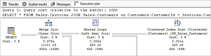
Figure 14-1 Sample query plan, showing a portion of the actual execution plan.
In Figure 14-1, on the Merge Join (Inner Join) operator, you can see that 11111 of 6654 rows were processed. The 6654 was the estimate, and 11111 was the actual number of rows.
Displaying live query statistics
Live query statistics, introduced in SSMS v16, are an excellent feature. With this feature, you can generate and display a “live” version of the execution plan using SSMS. It allows you to access live statistics on versions of SQL Server starting with SQL Server 2014. To use it, enable the Live Execution Statistics option for a connection via the Query menu in SSMS.
If you execute the query from the previous section with live query statistics enabled, you will see something like what’s shown in Figure 14-2. Notice that 1,684 of the estimated 6,654 rows have been processed by the Merge Join operator, and 93 rows have been processed by the Nested Loops (Left Semi Join) operator.
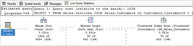
Figure 14-2 Sample live query statistics.
The Live Query Statistics window initially displays the execution plan more or less like the estimated plan, but fills out the details of how the query is being executed as it is processing it. If your query runs quickly, you’ll miss the dotted, moving lines and the various progress metrics, including the duration for each step and overall percentage completion. The percentage is based on the actual rows processed currently incurred versus a total number of rows processed for that step.
The Live Query Statistics window contains more information than the estimated query plan, such as the actual number of rows and number of executions, but less than the actual query plan. The Live Query Statistics window does not display some data from the actual execution plan such as actual execution mode, number of rows read, and actual rebinds.
Returning a live execution plan will noticeably slow down query processing, so be aware that the individual and overall execution durations measured will often be longer than when the query is run without the option to display live query statistics. However, it can be worth it to see where a query is hung up in processing.
If your server is configured correctly to do so, you can see the live query plan of executing queries in action by using the Activity Monitor in SSMS. In the Activity Monitor you can access the live execution plan by right-clicking any query in the Processes or Active Expensive Queries panes and selecting Show Live Execution Plan.
Note
Capturing live query execution statistics has some overhead, so use when it is valuable and not by default.
Permissions necessary to view execution plans
Not just anyone can view a query’s execution plans. There are two ways you can view plans, and they require different kinds of permissions.
If you want to generate and view a query plan, you will first need permissions to execute the query, even to get the estimated plan. Additionally, retrieving the estimated or actual execution plan requires the SHOWPLAN permission in each database referenced by the query. The live query statistics feature requires SHOWPLAN in each database, plus the VIEW SERVER STATE permission to see live statistics, so it cannot (and should not) be done by just any user.
It might be appropriate in your environment to grant SHOWPLAN and VIEW SERVER STATE permissions to developers. However, the permission to execute queries against the production database might not be appropriate in your regular environment. If that is the case, there are alternatives to providing valuable execution plan data to developers without production access. For example:
Providing database developers with saved execution plan (.sqlplan) files for offline analysis.
Configuring dynamic data masking, which might already be appropriate in your environment for hiding sensitive or personally identifying information for users who are not sysadmins on the server. Do not provide
UNMASKpermission to developers, however; assign that only to application users.Sometimes, an administrator may need to execute queries on a production server due to differences in environment or hardware, but be cautioned on all of what that means in terms of security, privacy, and so on.
- For more information on dynamic data masking, see Chapter 13, “Protect data through classification, encryption, and auditing.”
There are several tools that provide the ability to see existing execution plans. For example, Extended Events and Profiler can capture execution plans. Query reports in Activity Monitor, such as Recent Expensive Queries, also allow you to see the plan (if it is still available in cache). Dynamic management views (DMVs) that provide access to queries that executed (such as sys.dm_exec_cached_plans) or requests (sys.dm_exec_requests) will have a column named plan_handle that you can pass to the sys.dm_exec_query_plan DMV to retrieve the plan. To access plans in this manner, the server principal needs the VIEW SERVER STATE permission or must be a member of the sysadmin server role.
Finally, and perhaps the best way to view execution plans, is the Query Store, which is covered later in this chapter. For this, you need VIEW DATABASE STATE permissions or to be a member of the db_owner fixed role.
Understand execution plans
At this point, we have established the basics of what an execution plan is, where to find it, and what permissions you need to see it. After you have a graphical execution plan in front of you, you need a basic understanding of reading how the T-SQL statement was processed and how future queries that use this same plan will operate. The next several sections outline this process.
Read graphical execution plans
This section steps you through reviewing execution plans in SSMS and covers some of the most common things to look for.
Start an execution plan
First, start an execution plan. For our purposes, run a simple one, like for the following query:
SELECT Invoices.InvoiceID
FROM Sales.Invoices
WHERE Invoices.InvoiceID like '1%';
Figure 14-3 shows the resulting estimated query plan.
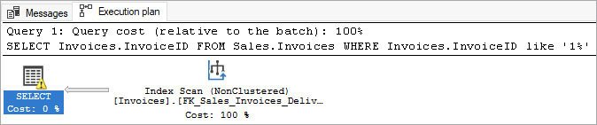
Figure 14-3 Simple query plan.
To display details for individual steps, position your pointer over a step in the execution plan to open a detailed tooltip-style window, much like the one shown in Figure 14-4. An interesting detail immediately should come to you when you look at the plan. It doesn’t say it is scanning the Sales.Invoices table, but rather an index. If an index has all the data needed to execute the query, the index “covers” the needs of the query, and the table’s other data structures are not touched.
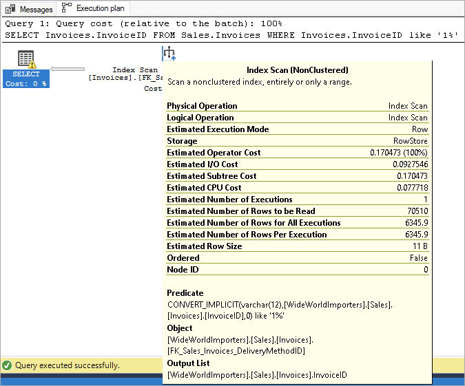
Figure 14-4 Simple query plan with statistics.
In SSMS, you can also select an operator in the execution plan and then press F4 or open the View menu and choose Properties Window to open its Properties window, where you will see the same estimated details.
Now, let’s get the actual execution plan, by pressing Ctrl+M or using one of the other methods discussed earlier. Execute the query and you will see the actual plan, as shown in Figure 14-5. It will be nearly identical to the estimate plan in Figure 14-3, but with more information.
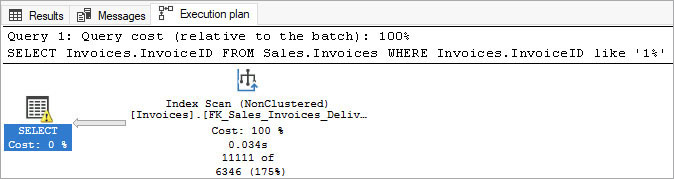
Figure 14-5 Actual execution plan for the sample query.
The first thing you should notice is that the query plan has a few more details. In particular, 11,111 of 6,346 rows were processed, where 6,346 is the estimated number of rows that would be returned by the query. This guess was based on statistics, which do not give perfect answers. When you are tuning larger queries, very large disparities between such guesses and the actual number require investigation.
Open the Properties pane and you’ll notice the returned estimate and actual values for some metrics, including Number of Rows, Executions, IO Statistics, and more. Look for differences in estimates and actual numbers here; they can indicate an inefficient execution plan and the source of a poor performing query. Your query might be suffering from a poorly chosen plan because of the impact of parameter sniffing or due to stale, inaccurate index statistics.
- We discuss parameter sniffing later in this chapter, including a new feature in SQL Server 2022 intended to avoid this classic problem, PSP optimization. Chapter 15 discusses index statistics.
Notice that some values, like Cost Information, contain only estimated values, even when you are viewing the actual execution plan. This is because the operator costs aren’t sourced separately; rather, they are generated the same way for both the estimated and actual plans and do not change based on statement execution. Furthermore, cost is not just comprised entirely of duration. You might find that some statements far exceed others in terms of duration, but not in cost.
Note
You can also review execution plans with a well-known third-party tool called Plan Explorer, a free download from https://www.sentryone.com/plan-explorer. It provides several additional ways to sort plan operators that are often helpful when working with very large query plans.
Start with the upper-left operator
The upper-left operator reflects the basic operation the statement performed—for example, SELECT, DELETE, UPDATE, INSERT, or any of the DML statements. (If your query created an index, you could also see CREATE INDEX.) This operator might contain warnings or other items that require your immediate attention. These typically appear with a small yellow triangle warning icon, over which you can position your mouse pointer to obtain additional details.
This was an intentional teaching opportunity! For example, in our sample plan, the SELECT operator is at the far left, and it has a triangle over it. You can see in the ToolTip that this is due to the following:
Type conversion in expression (CONVERT_IMPLICIT(varchar(12),[WideWorldImporters].
[Sales].[Invoices].[InvoiceID],0)) may affect "CardinalityEstimate" in query plan
choice, Type conversion in expression (CONVERT_IMPLICIT(varchar(12),[WideWorldImport
ers].[Sales].[Invoices].[InvoiceID],0)>='1') may affect "SeekPlan" in query plan choice.
In other words, we used a LIKE on an integer value, so the query plan is warning us that it cannot estimate the number of rows as well as it can if our WHERE clause employed integer comparisons to integers.
Select the upper-left operator and press F4 or open the View menu in SSMS and choose Properties Window. It lists some other things to look for. You’ll see warnings repeated in here, along with additional aggregate information.
Note
Yellow triangles on an operator indicate something that should grab your attention. The alert could tip you off to an implicit conversion—for example, a data-type mismatch that could be costly. Investigate any warnings reported before moving on.
Also look for the Optimization Level entry. This typically says Full. If the Optimization Level is Trivial, it means the Query Optimizer bypassed optimization of the query altogether because it was straightforward enough—for example, if the plan for the query only needed to contain a simple Scan or Seek operation along with the operation operator, like SELECT. If the Optimization Level is not Full or Trivial, this is something to investigate.
Look next for the presence of a value for Reason For Early Termination. This indicates the Query Optimizer did not spend as much time as it could have selecting the best plan. Here are a few possible reasons:
Good Enough Plan. This is returned if the Query Optimizer determined that the plan it picked was good enough to not need to keep optimizing.
Time Out. This indicates the Query Optimizer tried as many times as it could to find the best plan before taking the best plan available, which might not be good enough. If you see this, consider simplifying the query—in particular, by reducing the use of functions and potentially modifying the underlying indexes.
Memory Limit Exceeded. This is a rare and critical error indicating severe memory pressure on the SQL Server instance.
Look right, then read from right to left
Graphical execution plans build from sources (rightmost objects) and apply operators to join, sort, and filter data from right to left, eventually arriving at the leftmost operator. Among the rightmost objects, you’ll see scans, seeks, and lookups of different types. You might find some quick, straightforward insight into how the query is using indexes.
Each of the items in the query plan are referred to as operators. Each operator is a module of code that does a certain task to process data.
Two of the main types of operators for fetching data from a table or index are seeks and scans.
A seek operator finds a portion of a set of data through the index structure, similar to how you would use the index of a book to locate coverage of a specific topic. Seek operators are generally the most efficient operators and can rarely be improved by additional indexes. The seek operation finds the leaf page in the index, which contains the keys of the index, plus any included column data (which in the case of a clustered table will be all the data for the row).
If the leaf data contains everything you need, it means the operation was covered by the index. However, if you need more data than the index contains, a lookup operator will join with the seek operator using a join operator. This means that although the Query Optimizer used a seek, it needed a second pass at the table in the form of a lookup on another object, typically the clustered index, using a second seek operator.
Key lookups (on clustered indexes) and RID lookups (on heaps) are expensive and inefficient, particularly when many rows are being accessed. These lookups can add up to a very large percentage of the cost of a query.
If key lookup operators are needed frequently, they can usually be eliminated by modifying the index that is being scanned. For instance, you could modify an existing nonclustered index to include additional columns. For an example, see the section “Design rowstore nonclustered indexes” in Chapter 15.
The other typical data source operator is a scan. Scan operations aren’t great unless your query is intentionally returning a large number of rows out of a table or index. Scans read all rows from the table or index, which can be very inefficient when you need to return only a few rows, but more efficient when you need many rows. Without a nonclustered index with a well-designed key (if one can be found) to enable a seek for the query, a scan might be the Query Optimizer’s only option. Scans can be ordered if the source data is sorted, which is useful for some joins and aggregation options.
Scans on nonclustered indexes are often better than scans on clustered indexes, in part due to what is likely a smaller leaf page size, because a nonclustered index doesn’t usually have all the columns on the leaf page. Nonclustered indexes suffer from the same issues with key lookups.
Note
Very few queries are important enough to deserve their own indexes. Think “big picture” when creating indexes. If you create a new index for every slow query, the accumulated weight of nonclustered indexes will begin to slow writes to the table. As a guiding principle, more than one query should benefit from any new nonclustered index. Avoid redundant or overlapping nonclustered indexes. See Chapter 15 for more information on creating nonclustered indexes, including “missing” indexes.
Other types of scans include the following:
Table scan. This indicates that the table has no clustered index. Chapter 15 discusses why this is probably not a good idea.
Index scan. This scans the rows of an index, even the included columns of the index, for values.
Remote scan. This includes any object that is preceded by “remote,” which is the same operation but over a linked server connection. You troubleshoot these the same way, but potentially by making changes to the remote server instead. An alternative to linked server connections that might be superior in many cases is PolyBase. PolyBase can use T-SQL to query a variety of external data sources, including nonrelational and other relational data sources. Like a linked server, PolyBase accomplishes this by reading the data in place without data movement, or “virtualizing” the data.
- For more details on PolyBase, see Chapter 7.
Constant scan. These appear when the Query Optimizer deals with scalar values, repeated numbers, and other constants. These are necessary operators for certain tasks and generally not actionable from a performance standpoint.
Columnstore index. This is an incredibly efficient operator when you are working with lots of rows but relatively few columns, and likely will outperform a clustered index scan or index seek where millions of rows, for example, must be aggregated. There is no need to create a nonclustered index to replace this operator unless your query is searching for a few rows.
The weight of the lines connecting operators tells part of the story, but isn’t the full story
SQL Server dynamically changes the thickness of the gray lines to reflect the actual number of rows. You can get a visual idea of where the bulk of data is coming from by observing the pipes (they look like arrows pointing to the left), which draw your attention to the places where performance tuning could have the biggest impact. If you hover over the line in your query plan, you can see the rows transmitted in each step. (See Figure 14-6.)
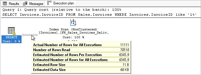
Figure 14-6 Showing the number of rows read and the estimated metrics in the query plan.
The visual weight and the sheer number of rows does not, however, directly translate to cost. Look for where the pipe weight changes from light to heavy, or vice versa. Be aware of when bolder pipes are joined or sorted.
Operator cost share isn’t the full story, either
When you run multiple queries, the cost of a query relative to the batch is displayed in the query execution plan header. The batch cost relative to the rest of the operators in the statement is displayed within each plan. SQL Server uses a cost-based process to decide which query plan to use.
When optimizing a query, it is usually useful to start with the costliest operators. But deciding to address only the highest-cost single operator in the execution plan might be a dead end.
Look for join operators and understand the different algorithms
As you read from right to left in a query of any complexity, you’ll likely see the paths meet at a join operator. Two tables, indexes, or the output from another operator can be joined together. There are three types of join operators to be aware of, particularly because they represent where a large percentage of the cost of an execution plan stems from: merge join, hash match, and nested loop. Any one of these can be the fastest way to join two sets of data, depending on the size of the sets, whether they are indexed, and whether they are sorted already (and if not, whether it would be too costly to sort them with a sort operator).
Note
There is also an adaptive join operator, first introduced in SQL Server 2017, which allows the Query Optimizer to situationally choose between the hash match and nested loop operators. This is mentioned again in the “Intelligent query processing” section later in this chapter.
A merge join operator merges two large, sorted sets of data. The query processor can scan each set, in order, matching rows from each table with a single pass through the sets. This can be quite fast, but the requirement for ordered sets is where the cost comes in. If you are joining two sets that are keyed on the same column, they are then sorted, so two ordered scans can be merged. The Query Optimizer can choose to sort one or both inputs to the merge join, but this is often costly.
Hash match is the join operator used to join two large sets, generally when there is no easily usable index and sorting is too costly. As such, it has the most overhead, because it creates a temporary index based on an internal hashing algorithm to bucketize values to make it easier to match one row to another. This hash structure is in memory if possible, but might spill onto disk (using tempdb). The presence of a hash join is not necessarily a bad thing; just know that it is the least efficient algorithm to join two data set, precisely because they are not suited for the other two operators.
Note
When the Query Optimizer does something that seems weird, like sort sets of data for an internal operation like a join, it is usually because it has calculated that for the design of your database, this is the best way to do it. As discussed, with complex queries, it sometimes take too long to find the absolute best way to process the query. And sometimes, the plans are suboptimal—for example, where statistics are not up to date. This is one reason to make sure plans have full optimization.
The most efficient join algorithm is the one that sounds the least optimized: nested loops. This join algorithm is the basic row-by-row processing that people preach about you as a programmer never doing. It takes one row in one input and searches the other input for values that meet the join criteria. When joining two sets together, one is indexed on the join key, and doesn’t need to fetch additional data using a key lookup. Nested loops are very fast. The additional operators were implemented to support larger, ideally reporting-style, workloads.
Each of the following options could reduce the cost of a join operator.
There might be an opportunity to improve the indexing on the columns being joined, or perhaps, you have a join on a compound key that is incompletely defined. Look for common joins in queries—can an index be crafted to match?
In the case of a merge join, you might see a preceding sort operator. This can be an opportunity for you to sort the data already sorted according to how the merge join requires the data to be sorted. If this is a composite key, perhaps change the ASC/DESC property of an index key column, or create a new nonclustered index with columns sorted differently. The result could result in a new execution plan without the cost of the sort operator.
Filter at the lowest level possible. Perhaps a
WHEREclause could exist in a subquery instead of at the top level of the query, or in the definition of a derived table or common table expression (CTE) instead of in the subsequent query.Hash operators are the most expensive. Reducing the row counts going into a hash match or hash join could allow the Query Optimizer to use a less memory-intensive and less costly join operator.
Nested loops are often necessitated by key lookups and are sometimes quite costly. Address them with a new or modified nonclustered index to eliminate the nearby key lookup, or to make an accompanying index seek more capable.
Look for parallel icons
The left-pointing pair of arrows in a yellow circle shown in Figure 14-7 indicate that this operator has been run with a parallel-processing execution plan. We talk more about parallelism later in this chapter; the important thing here is to be aware that your query has gone parallel.
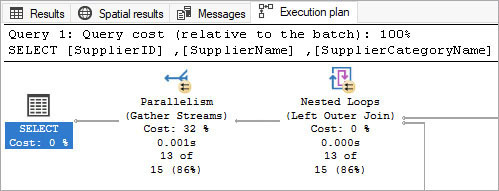
Figure 14-7 The parallel indicator on a clustered index scan operator.
This doesn’t mean multiple sources or pipes are being read in parallel; rather, it means the work for individual tasks has been broken up behind the scenes. The Query Optimizer decided it was faster if your workload was split up and run into multiple parallel streams of rows. Typically, this is a good thing, but at scale, excessive parallelism can lower overall performance.
- We discuss parallelism in more detail later in this chapter in the section “Understand parallelism.”
You might also see one of the three different parallelism operators—distribute streams, gather streams, and repartition streams—each of which appear only for parallel execution plans.
Understand cardinality estimation
When a query plan is being generated, one of the most important factors you will deal with is the cardinality estimation (CE). Cardinality is defined as the number of items in a set (hence, a cardinal number is a non-negative integer). The importance of cardinality estimation cannot be overstated and is analogous to how you might do a task. If you own an e-commerce store and ship three products a week, you might be able to walk two miles with your stack of packages to the post office at the end of the week and be efficient enough. If you must ship 300,000 products a day, however, the net effect of each product being shipped needs to be the same, but the way you achieve this must be far more optimized and include more than just one person.
SQL Server makes the same choices. You join table X with table Y on column ID. If X has 1,000 rows, and Y has 10, the solution is easy. If they each have a billion rows, and you are looking for a specific value in table X—say, value = 'Test'—there are many choices to make. How may rows in X have a value of 'Test'? And once you know that value, how many values of ID in X will match ID values in Y?
This estimation is done in two ways. The first is with guesses based on histograms of the data. The table is scanned when creating statistics. Statistics are created by executing UPDATE STATISTICS or through the automatic gathering of statistics that occurs as data changes, based on the AUTO_UPDATE_STATISTICS database setting.
Take the first case, where the tables are small. The engine stores a histogram that has something like what’s shown in Table 14-5.
Table 14-5 Sample histogram of a small table
RANGE_HI_KEY | RANGE_ROWS | EQ_ROWS | DISTINCT_RANGE_ROWS | AVERAGE_RANGE_ROWS… |
Smith | 400 | 200 | 20 | 10 |
Tests | 200 | 120 | 23 | 5 |
From this, the number of rows equal to 'Test' can be guessed to be less than 400 because Test is between Smith and Tests; less than 200, because approximately 200 rows matched Smith; and approximately 10 matches because there are approximately 20 distinct values. Exactly how this estimation is done is proprietary, but it is important to keep your statistics up to date using maintenance methods. (See Chapter 8 for more details on proper upkeep of SQL Server.)
From SQL Server 7.0 to SQL Server 2012, the same CE algorithms were used. However, since SQL Server 2014, Microsoft has been significantly tweaking the cardinality estimator with each release. And now, in SQL Server 2022, the new CE feedback feature allows SQL Server to automatically adapt query plans based on the estimate and actual number of rows processed, enhancing performance stability and automating an otherwise complex troubleshooting exercise.
- CE feedback is discussed later in this chapter. You can find out more at https://learn.microsoft.com/sql/relational-databases/performance/intelligent-query-processing-feedback#cardinality-estimation-ce-feedback.
The problem with cardinality estimation is that it is an inexact science. The guesses made are usually close enough, but sometimes can be off just enough to affect performance. Outdated statistics can lead to this, but that’s not the only explanation. Estimating filtered rowcounts in query plans is complex. That’s why it’s important that the new SQL Server 2022 “feedback” features allow SQL Server to quickly learn from mistakes.
There are a few methods to control which cardinality estimator is used. The first is to use the database’s compatibility level, like with this command to use the SQL Server 2022 cardinality estimator:
ALTER DATABASE [db_name] SET COMPATIBILITY_LEVEL = 160;Or you can elect to go backward and use the legacy SQL Server 2012 compatibility level:
ALTER DATABASE [db_name] SET COMPATIBILITY_LEVEL = 110;Changing the database’s compatibility level is often an unnecessary or drastic change. In your testing, consider keeping your modern compatibility level and reverting only to the legacy cardinality estimator (which pre-dated SQL Server 2014):
ALTER DATABASE SCOPED CONFIGURATION SET LEGACY_CARDINALITY_ESTIMATION = ON;Here also, reverting to the legacy cardinality estimator can be too drastic a change for the entire database. In compatibility level 130 (SQL Server 2016) and higher, there is a query hint you can use to modify an individual query to use legacy cardinality estimation (CE version 70):
SELECT …
FROM …
OPTION (USE HINT ('FORCE_LEGACY_CARDINALITY_ESTIMATION'));
What if you cannot modify the query to use the OPTION syntax because it resides deep within a business intelligence suite, an ETL tool, or third-party software? SQL Server 2022 has a solution for you: Identify the query in Query Store metadata and then provide a Query Store hint, shaping the query without altering any code. For example:
EXEC sys.sp_query_store_set_hints @query_id= 555,
@query_hints = N'OPTION(USE HINT(''FORCE_LEGACY_CARDINALITY_ESTIMATION''))';
In this example, the Query Store is used to identify a specific problematic query, which had been assigned query_id 555. This new SQL Server 2022 feature is only available when Query Store is enabled for the database, which we recommend.
Note
Query Store is enabled by default for all new databases on SQL Server 2022.
- For more information about Query Store hints, see the “Query Store hints” section later in this chapter.
For the most part, we suggest using the latest cardinality estimator possible, and addressing issues in your queries, but realize this is not always a feasible solution.
- For more information, including how to tell which version of cardinality estimation was used, see https://learn.microsoft.com/sql/relational-databases/performance/cardinality-estimation-sql-server.
- For more details, see Chapter 19, “Migrate to SQL Server solutions in Azure,” where we discuss using QTA for migrations. Also check out this lab that Microsoft created: https://github.com/microsoft/tigertoolbox/blob/master/Sessions/Winter-Ready-2019/Lab-QTA.md.
Understand parameterization and parameter sniffing
SQL Server parameterization occurs when the Query Optimizer detects values (such as the search criteria of a WHERE clause statement) that can be parameterized. For instance, the statements in a stored procedure are parameterized from the definition.
A query can be parameterized when it meets certain conditions. For example, a query might have values that could take on multiple values. A query such as
SELECT Value From TableName WHERE Value = 'X';can be parameterized, and the literal 'X' replaced by a parameter, much like if you were writing a stored procedure. This type of automatic parameterization is the default, referred to as simple parameterization. (Prior to SQL Server 2005, this was named auto-parameterization.)
The criteria for a query to qualify for simple parameterization are complex and lengthy. For example, a query where you reference more than one table will not be parameterized. If you change the PARAMETERIZATION database setting to FORCED, more complex queries will be parameterized. Object-Relational Mapping (ORM) frameworks like Entity Framework (EF) are likely to generate many queries that are too sophisticated for simple parameterization. With load testing, you could determine that your EF application could benefit from forced parameterization.
You can also rewrite a query to ensure it will get a parameterized plan by using a variable:
DECLARE @Value varchar(10) = 'X';
SELECT Value From TableName WHERE Value = @Value;
This query will be parameterized no matter how complex it is. There are additional ways a query will be parameterized through client APIs, but the best way to parameterize your queries is with stored procedures.
Note
Instead of complex procedurally developed queries coming out of object-relational mappers (ORMs) like Entity Framework in ADO.NET, consider stored procedures for application create, read, update, and delete (CRUD) operations. Stored procedures provide superior parameterization for security and cached execution plan reusability.
Simple parameterization is extraordinarily valuable, but also sometimes frustrating. With parameterization, it’s possible for two potentially helpful or potentially problematic conditions to occur:
You can reuse a query plan for multiple queries for which the query text is exactly the same, except for parameterized values. That’s helpful!
The same query could use the same execution plan for two different values of a parameter, resulting in vastly different performance. That’s problematic for one of the two values.
For example, you might create the following stored procedure to fetch orders placed for goods from a certain supplier:
CREATE OR ALTER PROCEDURE Purchasing.PurchaseOrders_BySupplierId
      @SupplierId int
AS
SELECT PurchaseOrders.PurchaseOrderID,
       PurchaseOrders.SupplierID,
       PurchaseOrders.OrderDate
 FROM   Purchasing.PurchaseOrders
WHERE  PurchaseOrders.SupplierID = @SupplierId;
The plan cached for this procedure will depend on the value that is passed in on the first compilation. For example, if the larger rowcount query (@SupplierID = 5) is used first and has its query plan cached, the query plan will choose to scan the clustered index of the table, because the value of 5 has a relatively high cardinality in the table. If the smaller rowcount query (@SupplierID = 1) is run first, its version of the plan will be cached, which will use an index seek and a key lookup. In this case, the plan with a seek and key lookup is far less efficient for very large row counts, but will be used for all values of the parameterized statement.
Here are a few advanced troubleshooting avenues to alleviate this scenario:
In SQL Server 2022, a new IQP feature, PSP optimization, actively adapts query plans to avoid this exact scenario. (More on this new feature at the end of this chapter, in the section “Intelligent query processing.”) Between PSP optimization and Query Store hints, SQL Server 2022 provides multiple superior options to deal with this classic problem.
Query Store hints, also new to SQL Server 2022, further allow administrators to tweak existing query plans with powerful hints, shaping query performance without the need for code changes. For example, even if you set simple parameterization at the database level, you could apply the query hint
PARAMETERIZATION FORCEDto individual complex queries. Query Store hints can specify this and many other query hints without changing the application code. With SQL Server 2022, you can even specify different Query Store hints on primary and secondary replicas of an availability group.You can use the
OPTIMIZE FORquery hint to demand that the query analyzer use a cached execution plan that substitutes a provided value for the parameters. You can also useOPTIMIZE FOR UNKNOWNto instruct the query analyzer to optimize for the most common value, based on statistics of the underlying data object. You can modify the code to useOPTIMIZE FORhints, or use the Query Store hints feature to apply a desiredOPTIMIZE FORhint without the need for code changes.The
RECOMPILEquery hint or procedure option does not allow the reuse of a cached plan, forcing a fresh query plan to be generated each time the query is run. Similarly, you can modify the code to useRECOMPILEhints, or use the Query Store hints feature to apply a desiredRECOMPILEhint without the need for code changes.You can use the Query Store feature (implemented with a GUI in SSMS and via stored procedures behind the scenes) to visually look at plan performance and force a query to use a specific plan currently in cache, using an easy graphical interface or T-SQL stored procedures. For more information, see the section “Leverage the Query Store feature” later in this chapter.
You can use the legacy plan guide feature (implemented via stored procedures) to guide the query analyzer to a plan currently in cache. You identify the plan via its
plan_handlesetting. Plan guides have been mostly replaced by the Query Store and Query Store hints feature, which provide a more granular and far easier way to tune query plans without code changes.Use the
USE PLANquery hint to provide the entire XML query plan forSELECTstatements. This is the least convenient option to override the query analyzer. Consider using the Query Store instead.An extreme solution is to disable parameter sniffing at the database level using the
PARAMETER_SNIFFING = OFFdatabase-scoped configuration option. This will cause all plans in the database to act like theOPTIMIZE FOR UNKNOWNhint has been provided.
Explore the procedure cache
The procedure cache is a portion of memory that contains query plans for statements that have been executed. New execution plans enter the procedure cache only when a statement is run. If the procedure cache already contains a plan matching a previous run of the current statement, the execution plan is reused, saving valuable time and resources. This is one reason complex statements can appear to run faster the second time they are run, in addition to the fact that data may be cached on a second execution.
The procedure cache is empty when the SQL Server service starts and grows from there. SQL Server manages plans in the cache, removing them as necessary under memory pressure. The size of the procedure cache is managed by SQL Server and is inside the memory space configured for the server in the Max Server Memory configuration setting. Plans are removed based on their cost and how recently they have been used. Smaller, older plans and single-use plans are the first to be cleared, though this formula of automatic plan cache maintenance is complex.
Note
If you are using SQL Server on Azure VMs, Azure SQL Database, or Azure SQL Managed Instance, look for the availability of newer memory optimized series of hardware. These are available for Azure VMs and in preview for various tiers and compute generations and offer a higher ratio of system memory to vCPUs.
Plans are compiled based on the state of the database and its objects when the plan is generated. Dramatic changes to underlying data might not cause an automatic plan recompilation, so recompiling a plan manually might help by creating a more optimized plan. Many data definition changes to tables referenced in the stored procedure will cause an automatic recompilation.
Clear the procedure cache
You might find that manually clearing the procedure cache is useful when performance testing or troubleshooting. Typically, you want to reserve this activity for preproduction systems.
There are a few common reasons to clear out cached plans in SQL Server. One is to compare two versions of a query or the performance of a query with different indexes; you can clear the cached plan for the statement to allow for proper comparison.
Note
While this can be a good thing to try, what you are testing is not only your query, but your hardware’s ability to fetch data from the disk. When you look at the output of SET STATISTICS IO ON, the Logical Reads measurement gives you an accurate comparison for two or more queries. The presence of Physical Reads tells you that data the query needed was not in cache. Higher amounts of physical reads indicate that the server’s ability to hold everything needed in RAM might not be sufficient.
You can manually flush the entire procedure cache, or individual plans in cache, with the following database-scoped configuration command, which affects only the current database context, as opposed to the entire instance’s procedure cache:
ALTER DATABASE SCOPED CONFIGURATION CLEAR PROCEDURE_CACHE;This command was introduced in SQL Server 2016 and is effectively the same as the DBCC FREEPROCCACHE command within the current database context. It works in both SQL Server and Azure SQL Database. DBCC FREEPROCCACHE is not supported in Azure SQL Database, and should be deprecated from your use going forward in favor of ALTER DATABASE.
Caution
We strongly recommend against clearing the procedure cache in a live production environment during normal business hours. Doing so will cause all new statements to have their execution plans compiled, dramatically increasing processor utilization, and potentially dramatically slowing performance.
You can also remove a single plan from cache by identifying its plan_handle and then providing it as the parameter to the ALTER DATABASE statement. Perhaps this is a plan you would like to remove for testing or troubleshooting purposes that you have identified with the script in the previous section:
ALTER DATABASE SCOPED CONFIGURATION CLEAR PROCEDURE_CACHE 0x06000700CA920912307B86
7DB701000001000000000000000000000000000000000000000000000000000000;
You can alternatively flush the cache by object type. This command clears cached execution plans that are the result of ad hoc statements and prepared statements (from applications, using sp_prepare, typically through an API):
DBCC FREESYSTEMCACHE ('SQL Plans');The advantage of this statement is that it does not wipe the cached plans from “programmability” database objects such as stored procedures, multi-statement table-valued functions, scalar user-defined functions, and triggers. The following command clears the cached plans from these types of objects:
DBCC FREESYSTEMCACHE ('Object Plans');Note
DBCC FREESYSTEMCACHE is not supported in Azure SQL Database.
You can also use DBCC FREESYSTEMCACHE to clear cached plans associated with a specific Resource Governor Pool, as follows:
DBCC FREESYSTEMCACHE ('SQL Plans', 'poolname');Analyze cached execution plans
You can analyze execution plans in aggregate starting with the sys.dm_exec_cached_plans DMV, which contains a column named plan_handle. The plan_handle column contains a system-generated varbinary(64) string that can be used with a number of other DMVs. As seen in the code example that follows, you can use the plan_handle to gather information about aggregate plan usage, obtain plan statement text, and retrieve the graphical execution plan itself.
You might be used to viewing the graphical execution plan only after a statement is run in SSMS, but you can also analyze and retrieve plans for queries executed in the past by using the following query against a handful of dynamic management objects (DMOs). These DMOs return data for all databases in SQL Server instances, and for the current database in Azure SQL Database. The following query can be used to analyze different aspects of cached execution plans. Note that this query might take a considerable amount of time as written, so you might want to pare down what is being output for your normal usage.
SELECT
    p.usecounts AS UseCount,
    p.size_in_bytes / 1024 AS PlanSize_KB,
    qs.total_worker_time/1000 AS CPU_ms,
    qs.total_elapsed_time/1000 AS Duration_ms,
    p.cacheobjtype + ' (' + p.objtype + ')' as ObjectType,
    db_name(convert(int, txt.dbid )) as DatabaseName,
    txt.ObjectID,
    qs.total_physical_reads,
    qs.total_logical_writes,
    qs.total_logical_reads,
    qs.last_execution_time,
    qs.statement_start_offset as StatementStartInObject,
      SUBSTRING (txt.[text], qs.statement_start_offset/2 + 1 ,
     CASE
         WHEN qs.statement_end_offset = -1
         THEN LEN (CONVERT(nvarchar(max), txt.[text]))
         ELSE qs.statement_end_offset/2 - qs.statement_start_offset/2 + 1 END)
     AS StatementText,
      qp.query_plan as QueryPlan,
      aqp.query_plan as ActualQueryPlan
FROM sys.dm_exec_query_stats AS qs
INNER JOIN sys.dm_exec_cached_plans p ON p.plan_handle = qs.plan_handle
OUTER APPLY sys.dm_exec_sql_text (p.plan_handle) AS txt

OUTER APPLY sys.dm_exec_query_plan (p.plan_handle) AS qp
OUTER APPLY sys.dm_exec_query_plan_stats (p.plan_handle) AS aqp
--tqp is used for filtering on the text version of the query plan
CROSS APPLY sys.dm_exec_text_query_plan(p.plan_handle, qs.statement_start_offset,
qs.statement_end_offset) AS tqp
WHERE txt.dbid = db_id()
ORDER BY qs.total_worker_time + qs.total_elapsed_time DESC;
The preceding code sorts queries by a sum of the CPU time and duration, descending, returning the longest running queries first. You can adjust the ORDER BY and WHERE clauses in this query to find, for example, the most CPU-intensive or most busy execution plans. Keep in mind that the Query Store feature, as detailed later in this chapter, will help you visualize the process of identifying the most expensive and longest running queries in cache.
As you will see after running in the previous query, you can retrieve a wealth of information from these DMOs, including statistics for a statement within an object that generated the query plan. The query plan appears as a blue hyperlink in SSMS’s Results to Grid mode, opening the plan as a new .sqlplan file. You can save and store the .sqlplan file for later analysis. Note too that this query might take quite a long time to execute as it will include a line for every statement in each query.
For more detailed queries, you can add code to search only for queries that have certain details in the plan—for example, looking for plans that have a reason for early termination value. In the execution plan XML, the reason for early termination will show in a node StatementOptmEarlyAbortReason. You can add the search conditions before the ORDER BY in the script, using the following logic:
and tqp.query_plan LIKE '%StatementOptmEarlyAbortReason%'Included in the query is sys.dm_exec_query_plan_stats, which provides the actual plan XML for a given plan_handle.
- More details on
sys.dm_exec_query_plan_statsare available at https://learn.microsoft.com/sql/relational-databases/system-dynamic-management-views/sys-dm-exec-query-plan-stats-transact-sql.
Permissions required to access cached plan metadata
The only permission needed to run the previous query in SQL Server is the server-level VIEW SERVER STATE permission, which might be appropriate for developers to have access to in a production environment because it does not give them access to any data in user databases.
In Azure SQL Database, because of the differences between the Basic/Standard and Premium tiers, different permissions are needed. In the Basic/Standard tier, you must be the server admin or Azure Active Directory Admin to access objects that would usually require VIEW SERVER STATE. In the Premium tier, you can grant VIEW DATABASE STATE in the intended database in Azure SQL Database to a user who needs permission to view the preceding DMVs.
Understand parallelism
Parallelism in query processing, and computing in general, is a very complex topic. Luckily, much of the complexity of parallelism in SQL Server is generally encapsulated from the DBA and programmer.
A query that uses parallelism, and one that doesn’t, can be the same query with the same plan (other than allowing one or more operators to work in parallel.) When SQL Server decides to split and stream data needed for requests into multiple threads, it uses more than one logical processor to get the job done. The number of different parallel threads used for the query is called the degree of parallelism (DOP). Because parallelism can never exceed the number of logical processors, naturally the maximum degree of parallelism (MAXDOP) is capped.
The main job of the DBA is to tune the MAXDOP for the server, database, and individual queries when the defaults don’t behave well. On a server with a mixed load of OLTP and analytics workloads, some larger analytics queries can overpower other active users.
MAXDOP is set at the server level using the server UI in SSMS, or more commonly using the sp_configure system stored procedure. Starting in SQL Server 2019, there is a MaxDOP tab in SQL Setup, which proposes an initial MAXDOP for your server configuration. In previous versions, the system default was 0 (allowing all processors to be used in a single statement).
Parallelism is a seemingly magical way to make queries run faster (most of the time), but even seeming like magic comes at a price. While queries might perform fastest in a vacuum going massively parallel, the overuse of parallelism creates a multithreading bottleneck at scale with multiple users. Split into too many different parts, queries slow down en masse as CPU utilization rises and SQL Server records increasing values in the CXPACKET wait type.
- We talk about
CXPACKEThere, but for more about wait type statistics, see Chapter 8.
Until SQL Server 2016, MAXDOP was only a server-level setting, a setting enforced at the query level, or a setting enforced for sessions selectively via the Resource Governor, an Enterprise edition feature. Since SQL Server 2016, the MAXDOP setting is also available as a database-scoped configuration. You can also use the MAXDOP query hint in any statement to override the database or server level MAXDOP setting.
- For more details on Resource Governor, see Chapter 3: “Design and implement an on-premises database infrastructure,” and Chapter 8.
Setting a reasonable value for MAXDOP will determine how many CPUs will be used to execute a query, but there is another setting to determine what queries are allowed to use parallelism: cost threshold for parallelism (CTFP). This enforces a minimum bar for query cost before a query can use a parallel execution plan. The higher the threshold, the fewer queries go parallel. This setting is low by default, but its proper setting in your environment depends on the workload and processor count. More expensive queries usually benefit from parallelism more than simpler queries, so limiting the use of parallelism to the worst queries in your workload can help. Similarly, setting the CTFP too high could have an opportunity impact, as performance is limited, queries are executed serially, and CPU cores go underutilized. Note that CTFP is a server-level setting only.
If large queries are already a problem for performance and multiple large queries regularly run simultaneously, raising the CTFP might not solve the problem. In addition to the obvious solutions of query tuning and index changes, it might be worth it to include the use of columnstore indexes for analytic queries and use MAXDOP as a hint instead to limit some very large queries from taking over your server.
A possible indication of parallelism being an issue is when the CXPACKET wait is a dominant wait type experienced over time by your SQL Server. You might need to adjust both MAXDOP and CTFP when performance tuning. You can also view the live and last wait types for a request using sys.dm_exec_requests. Make these changes in small, measured gestures, and don’t overreact to performance problems with a small number of queries. Use Query Store to benchmark and trend the performance of high-value and high-cost queries as you change configuration settings.
Another flavor of CPU pressure, and in some ways the opposite of the CXPACKET wait type, is the SOS_SCHEDULER_YIELD wait type. The SOS_SCHEDULER_YIELD is an indicator of CPU pressure, indicating that SQL Server was forced to share time, or “yield” to other CPU tasks, which might be normal and expected on busy servers. Whereas CXPACKET is the SQL Server complaining about too many threads in parallel, SOS_SCHEDULER_YIELD is the acknowledgement that there were more runnable tasks than available threads. In either case, you should adopt a strategy of reducing CPU-intensive queries and rescheduling or optimizing CPU-intensive maintenance operations. This is more economical than simply adding CPU capacity.
Force a parallel execution plan
You know how to specify MAXDOP = 1 to force a query not to use parallelism. What about forcing parallelism? You can use a query hint to force a statement to compile with a parallel execution plan. This can be valuable in troubleshooting, or to force a behavior in the Query Optimizer for experimentation, but is not usually a necessary or recommended option for live code.
Appending the following hint to a query will force a parallel execution plan, which you can see using the estimate or actual execution plan output options:
… OPTION(USE HINT('ENABLE_PARALLEL_PLAN_PREFERENCE'));Note
The presence of certain system variables or functions can force a statement to compile to be serial—that is, without any parallelism. This behavior will override the new ENABLE_PARALLEL_PLAN_PREFERENCE option.
The @@TRANCOUNT system variable forces a serial plan, as do any of the built-in error reporting functions, including ERROR_LINE(), ERROR_MESSAGE(), ERROR_NUMBER(), ERROR_PROCEDURE(), ERROR_SEVERITY(), and ERROR_STATE(). This pertains only to using these objects in a query. Using them in the same batch, such as in a TRY … CATCH handler, will not affect the execution plans of other queries in the batch.
Use advanced engine features to tune queries
In the past few versions of SQL Server and Azure SQL Database, the programmers building the Database Engine have started to add especially advanced features to go from the same cost-based optimizations we have had for many years, to tools that can sense when plans need to be adjusted before a DBA does. Not that any of these features will replace well-written code and a DBA who understands the architecture of how queries work, but as data needs explode, the more the engine can do for you, the better.
Internal improvements in SQL Server 2022
Microsoft has published a few details on some internal performance improvements that were introduced deep inside the Database Engine. Here is a summary of these advanced changes. None require an opt-in or deep understanding of the tech involved in order for you to benefit from them in SQL Server 2022.
Reduced buffer pool I/O promotions. There is a documented phenomenon involving the read-ahead mechanism that pulls data from storage into the buffer pool. To read more about this complex topic, see this old Microsoft blog post at https://learn.microsoft.com/archive/blogs/ialonso/the-read-ahead-that-doesnt-count-as-read-ahead. New to SQL Server 2022, the number of incidents where a single page would be promoted to an extent has been reduced. This makes SQL Server’s access of the physical I/O subsystem to populate memory more efficient. This change was delivered with SQL Server 2022 and pushed to Azure SQL Database and Azure SQL Managed Instance at the time of this writing.
Enhanced spinlock algorithms. Another complex topic from deep within the Database Engine improves the performance of SQL Server when multiple threads generate spinlocks. This is an oversimplification of a complex topic, of course, but the details on this performance tune are limited. This change was delivered with SQL Server 2022 and pushed to Azure SQL Database and Azure SQL Managed Instance at the time of this writing.
Virtual Log File (VLF) allocation improvements. In certain growth scenarios, the number of VLFs allocated to the transaction log was less efficient than it could have been. For small growth increments in small transaction log files, a single 64 MB VLF is created, instead of multiple VLFs. Over time, these VLF growth patterns make for a more efficient transaction log internal structure that benefits recovery and log truncation. For more details on the formulas involved here, visit https://learn.microsoft.com/sql/relational-databases/sql-server-transaction-log-architecture-and-management-guide#virtual-log-files-vlfs. This change was delivered with SQL Server 2022 and pushed to Azure SQL Database at the time of this writing.
Recent improvements to tempdb
Each of the past versions of SQL Server versions has introduced significant new features to improve the performance of the tempdb database. SQL Server 2022 introduces some key improvements to how tempdb works internally that do not require any configuration. You benefit from them immediately.
In SQL Server 2022, system page latches in tempdb have received concurrency enhancements. Both Global Allocation Map (GAM) and Shared Global Allocation Map (SGAM) pages received updates to improve concurrency, an extension of the concurrency improvements to Page Free Space (PFS) pages in tempdb that were introduced with SQL Server 2019. Also in SQL Server 2019, memory-optimized metadata in tempdb cure some specific bottlenecks at high scale having to do with how temporary objects can be created, modified, and destroyed.
- For more information, see Chapter 3.
Leverage the Query Store feature
The Query Store provides a practical history of execution plan performance for a single database, which persists even when the server has been restarted (unlike the plan cache itself, which is cleared, eliminating all the interesting data that one needs for tuning queries over time). It can be invaluable for the purposes of investigating and troubleshooting sudden negative changes in performance, allowing the administrator or developer to identify both high-cost queries and the quality of their execution plans, and especially when the same query has multiple plans, where one performs poorly and the other well.
Starting with SQL Server 2022, and likely to be a default in Azure SQL Database and Azure SQL Managed Instance in the near future, the Query Store is enabled and in read/write mode by default for new databases. Databases migrated to SQL Server 2022 retain their Query Store settings.
The Query Store is most useful for looking back in time toward the history of statement execution. It can also assist in identifying and overriding execution plans by using a feature similar to, but different from, the plan guides or Query Store hints feature. As discussed in the previous section, plan guides are used to override a query’s plan. Instead of plan guides, consider instead the Query Store’s ability to force plans, or the Query Store hints feature (introduced in SQL Server 2022 and Azure SQL Database) to shape query plans without code changes.
The Query Store allows you to find plans that are not working well, but only gives you the ability to force an entire plan that worked better from the history it has stored. The Query Store has a major benefit over legacy plan guides in that there is an SSMS user interface to access it, see the benefits, and find places where you might need to apply a new plan.
You see live Query Store data as it happens from a combination of both memory-optimized and on-disk sources. Query Store minimizes overhead and performance impact by capturing cached plan information to in-memory data structure. The data is flushed (persisted) to disk at an interval defined by Query Store, by a default of 15 minutes. The Disk Flush Interval setting defines how much Query Store data can be lost in the event of an unexpected system shutdown.
Note
Queries are captured in the context of the database where the query is executed. In the following cross-database query example, the query’s execution is captured in the Query Store of the WideWorldImporters sample database.
USE WideWorldImporters;
GO
SELECT * FROM
AdventureWorks.[Purchasing].[PurchaseOrders];
Microsoft delivered the Query Store to the Azure SQL Database platform first, and then to the SQL Server product. In fact, Query Store is at the heart of the Azure SQL Database Advisor feature that provides automatic query tuning. The Query Store feature’s overhead is quite manageable, tuned to avoid performance hits, and is already in place on millions of customer databases in Azure SQL Database.
The VIEW DATABASE STATE permission is all that is needed to view the Query Store data.
Initial configuration of Query Store
Query Store is identical between the Azure SQL Database and SQL Server in operation, but not in how you activate it. Query Store is enabled automatically on Azure SQL Database and all new databases starting with SQL Server 2022, but it is not automatically on for existing databases that you migrate to SQL Server 2022.
When should you enable Query Store? Enabling Query Store on all databases you have in your environment is a generally acceptable practice, as it will be useful in discovering performance issues in the future when they arise. You can enable Query Store via the database’s Properties dialog box, in which a Query Store page is accessible from the menu on the left, or you can turn it on via T-SQL by using the following command:
ALTER DATABASE [DatabaseOne] SET QUERY_STORE = ON;This will enable Query Store with the defaults; you can adjust them using the UI.
Note
As with almost any configuration task, while it is acceptable to use the UI the first few times, it will always be better to have a script in T-SQL or PowerShell to capture settings in a repeatable manner. Use the Script button in most SSMS UIs to output a script of what has changed when you are setting new values.
Query Store begins collecting data when you activate it. You will not have any historical data when you first enable the feature on an existing database, but you will begin to immediately see data for live database activity. You can then view plans and statistics about the plan in the Query Store reports.
In versions before SQL Server 2019, the default Query Store capture mode setting was ALL, which included all queries that were executed. In SQL Server 2019, this default has been changed to AUTO, which is recommended. The AUTO Query Store capture mode forgets queries that are insignificant in terms of execution duration or frequency. Further, the CUSTOM Query Store capture mode allows for more fine tuning that may become necessary on large and busy databases. While AUTO works fine for most servers, you can use custom capture policies to configure the tradeoff: the amount of history remembered by Query Store versus the amount of storage the Query Store consumes inside the user database.
The Query Store retains data up to two limits: a max size (1,000 MB by default), and a Stale Query Threshold time limit in days (30 by default). If Query Store reaches its max size, it cleans up the oldest data. Because Query Store data is saved in the database, its historical data is not affected by the commands we looked at earlier in this chapter to clear the procedure cache, such as DBCC FREEPROCACHE.
You should almost always keep the size-based cleanup mode set to the default, Auto. If not, when the max size is reached, Query Store will stop collecting data and enter read-only mode, which does not collect new data. If you find that the Query Store is not storing more historical days of data than your stale query threshold setting in days, increase the max size setting.
Troubleshoot with Query Store data
Query Store has several built-in dashboards, shown in Figure 14-8, to help you examine query performance and overall performance over recent history.
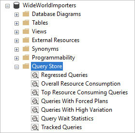
Figure 14-8 The SQL Server Object Explorer list of built-in dashboards available for Query Store in SSMS.
You can also write your own reports against the collection of system DMOs that present Query Store data to administrators and developers by using the VIEW DATABASE STATE permission.
- You can view the schema of the well-documented views and their relationships at https://learn.microsoft.com/sql/relational-databases/performance/how-query-store-collects-data.
On many of the dashboards, there is a button with a crosshairs symbol, as shown in Figure 14-9. If a query seems interesting, expensive, or is of high value to the business, you can select this button to view a new window that tracks the query when it’s running as well as various plans identified for that query.
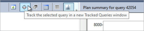
Figure 14-9 The Query Store toolbar at the top of the screen on many of the dashboards—in this example, the toolbar for the Regressed Queries report.
You can review the various plans for the same statement, compare the plans, and if necessary, force a plan that you believe is better than the Query Optimizer will choose into place. Compare the execution of each plan by CPU time, duration, logical reads, logical writes, memory consumption, physical reads, and several other metrics.
Most of all, the Query Store can be valuable by informing you when a query started using a new plan. You can see when a plan was generated and the nature of the plan; however, the cause of the plan’s creation and replacement is not easily deduced, especially when you cannot correlate to a specific DDL operation or system change. Query plans can become invalidated automatically due to large changes in statistics resulting from data inserts or deletes, changes made to other statements in the stored procedure, changes to any of the indexes used by the plan, or manual recompilation due to the RECOMPILE option.
As discussed in the upcoming “Query Store hints” section, forcing a statement (see Figure 14-10) to use a specific execution plan should not be a common activity. If you have access to the source code, work on a code change, only using a forced plan temporarily. For systems where you have no code access, you can use a Query Store hint for specific performance cases, problematic queries demanding unusual plans, and so on. Note that if the forced plan is invalid, such as an index changing or being dropped, SQL Server will move on without the forced plan and without a warning or error, although Query Store will still show that the plan is being forced for that statement. Note that once a plan has been forced for this statement (using the Force Plan button), the plan is displayed with a check mark.
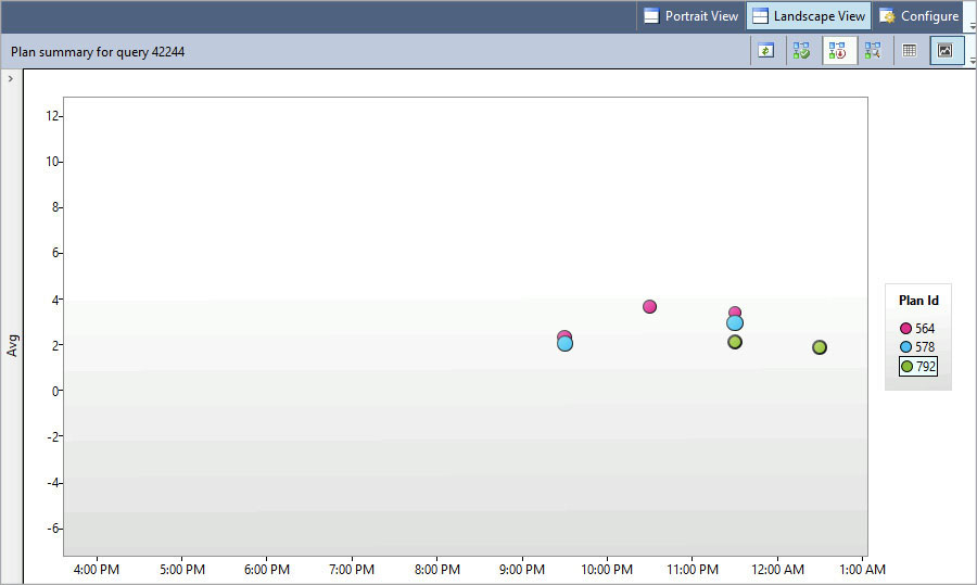
Figure 14-10 The Query Store records the query’s execution results.
Query Store hints
In past editions of this book, in this space, we’d discuss plan guides—an aging and well-documented feature that was inconvenient if not downright painful to implement. The new Query Store hints feature is a superior alternative to plan guides. Query Store hints provide powerful tools to shape queries without making code changes, giving administrators and developers options to modify query plans substantially and easily.
Query Store hints were in preview for Azure SQL Database and Azure SQL Managed Instance starting mid-2021, and later Microsoft brought the feature to SQL Server 2022. Like many of the new IQP features introduced in SQL Server 2022, Query Store hints require the Query Store to be enabled on the database. For this reason, you should strongly consider enabling, monitoring, and customizing the Query Store feature on every performance-sensitive database.
Query Store hints give administrators an easy replacement to the older plan guides feature, which was introduced in SQL Server 2005. You can use Query Store to force replacement plans into action. You can use Query Store hints to force hints into query plans. All require no code changes, giving administrators and developers options to modify query plans coming from third-party software, SSIS packages, and business intelligence tools.
With both plan guides and Query Store hints, you can influence a plan by simply adding a hint (a common example would be WITH RECOMPILE). This can be very useful if you have a plan that is being chosen by SQL Server that doesn’t work for you and you have no way to change the query code in question. Combined with new improvements around parameter sniffing thanks to PSP optimization, it is easy to achieve performance gains in SQL Server 2022.
Query Store is a more complete tuning solution than plan guides, capturing plans from the plan cache and tracking query performance with different plans over time. A suite of reports and graphical tools make it easy to investigate query performance. Like with plan guides, you can manually override the query plan chosen with a previously observed plan. Further, the automatic plan correction feature can automatically override a query plan with a previously observed plan that performed better. Automatic plan correction was introduced with SQL Server 2017.
This section reviews aspects of both tools to help guide you as to which tool to choose. Note, however, that tools that force a plan to override what the Query Optimizer has chosen are not considered the best approach to query tuning. If you have an application where you own the source code, forcing a plan might be good to do until you can make a change to code, but should not be your primary tuning tool. If it is a third-party application, you should work with your vendor on a proper solution, but these features will help you to get past a serious issue.
Use Query Store hints
Currently, like plan guides, Query Store hints are driven by T-SQL stored procedures and not accessible from within any GUI (yet). But the identification of queries can occur through the Query Store interface, through a unique key for all queries captured by the Query Store, query_id.
Caution
Query Store hints—like plan guides or forcing plans using USE PLAN or the Query Store—are an advanced troubleshooting technique and are not without some risk.
The following steps will detail how to back out of a Query Store hint quickly. Be prepared to observe and rollback any hints.
Identify a useful hint for the query, ideally by using a non-production performance testing environment with similar hardware and data scale.
Identify the Query Store–assigned
query_idfor the query. Note that thequery_idwill be different on different instances of SQL Server.Use
sys.sp_query_store_set_hintsto apply a hint. Most query hints are supported. For example, to apply theMAXDOP 1hint toquery_id1234, use the following:EXEC sys.sp_query_store_set_hints @query_id= 1234, @query_hints = N'OPTION(MAXDOP 1)';- For a complete list of supported query hints, review the Microsoft Docs article for
sys.sp_query_store_set_hintsat https://learn.microsoft.com/sql/relational-databases/system-stored-procedures/sys-sp-query-store-set-hints-transact-sql#supported-query-hints.
You can specify more than one query hint in a Query Store hint, just as you would in the
OPTIONclause of any T-SQL query. For example, to specifyMAXDOP 1and the pre-SQL Server 2014 cardinality estimator, use this:EXEC sys.sp_query_store_set_hints @query_id= 1234, @query_hints = N'OPTION(MAXDOP 1, USE HINT(''FORCE_LEGACY_CARDINALITY_ESTIMATION''))';The Query Store hint takes effect immediately and adds three attributes to the execution plan XML:
QueryStoreStatementHintId,QueryStoreStatementHintText, andQueryStoreStatementHintSource. If you’re curious, you can review these to see the Query Store hint in action, and prove the hint altered the query without code changes.Observe and confirm that your hint is helping the query’s execution. Confirm the Query Store hint(s) currently in place for your query as follows:
SELECT * FROM sys.query_store_query_hints
WHERE query_id = 1234;
Remove the Query Store hint when necessary with
sys.sp_query_store_clear_hints. (You want to prepare for this ahead of time.)EXEC sys.sp_query_store_clear_hints @query_id = 1234;Set yourself a reminder to reevaluate any Query Store hints on a regular basis. Data distributions change and the winds of fate blow. Changes to underlying data and concurrent server workloads might cause Query Store hints to generate suboptimal execution plans in the future.
If you set a Query Store hint, it will overwrite any existing hint for that
query_id. Query Store hints will override other hard-coded statement level hints and plan guides, but you should avoid conflicting instructions as they could be confusing for others in your environment.
Automatic plan correction
Automatic plan correction is a feature that relies on the Query Store to detect and revert query duration regression. For example, suppose a commonly executed query normally runs in 100 milliseconds, but then changes execution plans and starts finishing in 2 minutes. Instead of waiting for complaints of slow performance, the engine can notice this regression and deal with it. SQL Server 2017 introduced this feature to the on-premises versions of the Database Engine, and was originally released for Azure SQL Database.
A typical use case is to view the regressed queries report in Query Store, identify a query that has regressed in duration, and then force a better past execution plan into use. With automatic plan correction enabled, the database can detect plan regression and take action to force the previous plan back into action, automatically. The sample syntax for enabling automatic plan correction is below:
ALTER DATABASE WideWorldImporters SET AUTOMATIC_TUNING (FORCE_LAST_GOOD_PLAN = ON );The sys.dm_db_tuning_recommendations DMO captures plan recommendations based on query performance regression. This doesn’t happen immediately—the feature has an algorithm that requires several executions before regression is identified. When a recommendation appears in sys.dm_db_tuning_recommendations, it includes a large amount of diagnostic data, including a plain-language explanation for the recommendation to be generated, and a block of JSON data containing diagnostic information.
- A sample query to parse this data is available at https://learn.microsoft.com/sql/relational-databases/automatic-tuning/automatic-tuning.
Intelligent query processing
Intelligent query processing (IQP) is not a tool or a GUI option, but rather a suite of behind-the-scenes features that make the processing of queries more efficient. Many are specific to the database compatibility version; you don’t benefit from them in an older version compatibility. Some features help to pick or adapt a query plan to current conditions. Others are just straight up changes to how the Database Engine uses long existing query constructs. In every case, the goal of IQP features is to improve the way queries are processed without code changes.
The remainder of this chapter covers the new IQP features in SQL Server 2022 and some of the most significant features in recent versions, though a review of the complete list of the IQP suite of performance features is worthwhile.
- For more information, see https://learn.microsoft.com/sql/relational-databases/performance/intelligent-query-processing.
Batch mode on rowstore
One of the features added, along with columnstore indexes, in SQL Server 2012 was a type of processing known as batch mode. Columnstore indexes were built to process compressed rowgroups containing millions of rows. A new processing mode was needed when the heuristics told the query processor it would be worthwhile to work on batches of rows at a time.
- For more details on batch and row mode processing, see https://learn.microsoft.com/sql/relational-databases/query-processing-architecture-guide.
Starting with SQL Server 2019 and included in Azure SQL Database, this feature was extended to work for certain types of queries with row store tables and indexes as well as columnstore tables and indexes. A few examples:
Queries that use large quantities of rows in a table, often in analytical queries touching hundreds of thousands of rows.
Systems that are CPU bound in nature. (I/O bottlenecks are best handled with a columnstore index.)
The feature is enabled when the compatibility level is at least 150. Though unusual, if you find it is harming performance, you can turn it off using ALTER DATABASE without lowering the compatibility level:
ALTER DATABASE SCOPED CONFIGURATION SET BATCH_MODE_ON_ROWSTORE = OFF;Instead of changing this setting for the database, you could disallow this feature for a specific query, perhaps one that touches large number of rows. You can use the query hint ALLOW_BATCH_MODE. For example:
SELECT …
FROM …
OPTION(USE HINT('ALLOW_BATCH_MODE'));
Note
Columnstore and rowstore indexes continue to exchange advantageous features. In SQL Server 2022, ordered clustered columnstore indexes arrived, a feature first introduced for Azure Synapse Analytics. We cover this more in the next chapter.
Cardinality estimation (CE) feedback
Similar to other feedback features, CE feedback allows the Query Optimizer to adapt to changes in query performance based on suboptimal CE. CE estimates the total number of rows in the various stages of a query plan. (Constraints and key relationships between tables can help inform and shortcut estimation, another good reason to put them in place.)
CE feedback is a process by which the Query Optimizer learns by modeling query behavior over time. This feature requires both compatibility level 160 (for SQL Server 2022) and the Query Store to be enabled for the database.
In the past, the cardinality estimator and the database’s compatibility level were closely linked. (Changes in SQL Server 2014 improved the cardinality estimator in most but not all cases, with severe impacts when it missed.) CE feedback does not change the database compatibility level for the query, but makes incremental corrections via the Query Store hint feature.
- For more about Query Store hints, see the “Understand cardinality estimation” section earlier in this chapter.
At the time of this writing, CE feedback is not yet available in Azure SQL Database or Azure SQL Managed Instance, but should be available in the near future.
SQL Server 2022 also added a persistence feature for CE feedback. Persistence helps CE feedback avoid poor adjustment decisions by remembering query information, even if a plan is evicted from cache. Using the Query Store, estimates can be considered over multiple query executions.
Degree of parallelism (DOP) feedback
DOP feedback has perhaps the biggest impact of all the feedback features introduced to make SQL Server more adaptive to observed performance. The ability for the Query Optimizer to analyze and adapt to observed query performance and make changes to parallelism with each query execution is a powerful self-tuning feature.
DOP feedback is introduced with SQL Server 2022, and requires the Query Store feature to be enabled. Further, the DOP_FEEDBACK database scoped configuration can be enabled or disabled if necessary.
Instead of worrying about optimizing the database’s MAXDOP for the most important parts of a workload, DOP feedback automatically adjusts parallelism for repeating queries with the goal of increasing overall concurrency and reducing wait times. Smartly, DOP feedback excludes some wait types that are not relevant to this part of query performance, such as buffer latch, buffer IO, and network IO waits.
DOP feedback adjusts queries automatically by adding the MAXDOP query hint, but never at a value exceeding the database’s MAXDOP setting. You might consider exploring the performance gains with DOP feedback in a different (higher) MAXDOP setting for your server or database in SQL Server 2022.
At the time of this writing, DOP feedback is not yet available in Azure SQL Database or Azure SQL Managed Instance, but should be available in the near future.
SQL Server 2022 also added a persistence feature for DOP feedback. Persistence helps the DOP feedback feature avoid poor adjustment decisions by remembering query information, even if a plan is evicted from cache. Using the Query Store, optimal parallelism can be considered over multiple executions.
Memory grant feedback
When a query executes, it uses some amount of memory. Memory grant feedback lets future executions of the same query know if the memory granted for the execution was too much or too little, so it can adjust future executions. Memory grant feedback was introduced in SQL Server 2017 for batch mode executions, and in SQL Server 2019 for row mode executions.
If for some reason you want to disable this feature in a database, you can do so without lowering the database compatibility level using the following statements:
-- SQL Server 2017
ALTER DATABASE SCOPED CONFIGURATION SET DISABLE_BATCH_MODE_MEMORY_GRANT_FEEDBACK = OFF;
-- Azure SQL Database, SQL Server 2019 or later
ALTER DATABASE SCOPED CONFIGURATION SET BATCH_MODE_MEMORY_GRANT_FEEDBACK = OFF;
For row mode queries, this feature is controlled using:
ALTER DATABASE SCOPED CONFIGURATION SET ROW_MODE_MEMORY_GRANT_FEEDBACK = OFF;
SQL Server 2022 further enhances memory grant feedback with two additional features: persistence and percentile improvement. Both are intended to help the Query Optimizer avoid expensive memory spills by accurately estimating (or at worst, overestimating) the amount of memory needed for crucial parts of an execution plan.
Memory grant feedback persistence allows SQL Server to remember query memory grant information even if a plan is evicted from cache. Using the Query Store, feedback can be considered over multiple executions. Persistence also applies to CE feedback and DOP feedback, as stated.
Memory grant feedback percentile adjustment allows the memory grant adjustment to examine the recent history of query execution, not just the most recent execution. The complex calculation now includes the 90th percentile of past memory grants over time. The percentile adjustment only applies to memory grant feedback.
When the new Query Store for secondary replicas feature is enabled, memory grant feedback is replica aware and can help primary and secondary replica workloads differently.
Parameter Sensitive Plan optimization
Parameter Sensitive Plan (PSP) optimization, new in SQL Server 2022, addresses the age-old problem of queries getting a suboptimal execution plan when the value of a filter wildly changes the result sets. PSP solves the problem in an intuitive way: by allowing more than one cached execution plan to be saved for a single query.
Imagine a search query for sales, filtered on customer, where customer_id = @customer_id. Customer 1 has been purchasing goods for decades, and has millions of invoice line items. Customer 2 is a new customer with a single invoice. In previous versions of SQL Server, should the execution plan for customer 2 become the execution plan for this search query, performance of the query on customer 1 would be poor. This is because the operators chosen for the execution plan would be unlikely to scale from one row to millions of rows in the result set.
Previous solutions required an understanding of query parameterization and the application of a variety of strategies, including cache preparation, synthetically calling queries with their largest filter parameters using the OPTIMIZE FOR query hint, or using plan guides. Between PSP optimization and Query Store hints, SQL Server 2022 provides multiple superior options to deal with this classic problem. PSP optimization uses a complex set of instructions that require a significant amount of performance data to act and cache a different plan, in an effort to minimize memory utilization associated with unnecessary plan retention.
PSP optimization is part of the database compatibility level 160 feature set, so be sure to update the compatibility level for any databases migrated up to SQL Server 2022. Query Store is not required for PSP optimization, but it is recommended.
If for some reason you need to disable PSP optimization, you can do so without lowering the database compatibility level with the PARAMETER_SENSITIVE_PLAN_OPTIMIZATION database-scoped configuration option.
- For a deep dive on the internals of PSP optimization, see https://learn.microsoft.com/sql/relational-databases/performance/parameter-sensitivity-plan-optimization.
Caution
A known bug in an early public preview of PSP optimization in SQL Server 2022 raised an error when you did not specify two part names (schemaname.objectname) in stored procedures that were not in the dbo schema. While this bug has been fixed, it’s just another reminder that a good best practice is to always specify two-part names in your T-SQL code, even for objects in the dbo schema.
Table variable deferred compilation
Table variable deferred compilation was introduced in SQL Server 2019 to deal with the glaring lack of statistics for a table variable at compile time. Previously, SQL Server defaulted to a guess of one (1) row for the number of rows in the table variable. This provided poorly performing plans if the programmer had stored any significant number of rows in the table variable.
Similarly, an IQP feature introduced in SQL Server 2017 called interleaved execution improved the performance of multi-statement table-valued functions. Interleaved execution let the Query Optimizer execute parts of the query during optimization to get better estimates, because if your multi-statement table-valued function is going to output 100,000 rows, the plan needs to be considerably different.
Instead of using the guess of 1 to define the query plan, table variable deferred compilation waits to complete the actual plan until the table variable has been loaded the first time, and then the rest of the plan is generated.
Note
Table variable optimizations do not make table variables the best choice for large numbers of rows. Table variables still lack column statistics, a key difference between them and temp tables (prefixed with # or ##) that can make temp tables far superior for large rowsets.
T-SQL scalar user-defined function (UDF) inlining
A common culprit of poor performance in custom applications is user-defined functions (UDFs). Every programmer who has taken any class in object-oriented programming (OOP) instinctively desires to modularize or de-duplicate their code. So, if you have a scenario in which you want to classify some data (say, something simple like CASE WHEN 1 THEN 'True' ELSE 'False' END), it makes sense from a programmer’s perspective to bundle this up into a coded module (code reuse). However, UDFs can become a bear trap at scale for application performance.
Introduced in SQL Server 2019, scalar UDF inlining alleviates some of the performance hit introduced by UDFs at scale; it’s an automatic, no-code-change-necessary, performance boost. This is a complex fix that substitutes scalar expressions or subqueries in the query during query optimization. Throughout the post-RTM life of SQL Server 2019, cumulative updates added complexity, issue fixes, and restrictions to UDF inlining.
Example of scalar UDF inlining
To demonstrate UDF inlining, we created the following overly simple UDF in the WideWorldImporters sample database:
USE WideWorldImporters;
GO
CREATE SCHEMA Tools;
GO
CREATE FUNCTION Tools.Bit_Translate
(@value bit)
RETURNS varchar(5)
AS
BEGIN
     RETURN (CASE WHEN @value = 1 THEN 'True' ELSE 'False' END);
END;
To demonstrate, execute the function in the same query twice: once in SQL Server 2017 (14.0) database compatibility level, before scalar UDF inlining was introduced, and again with SQL Server 2022 (16.0) database compatibility level behavior.
SET STATISTICS TIME ON;
ALTER DATABASE WideWorldImporters SET COMPATIBILITY_LEVEL = 140; --SQL Server 2017
GO
SELECT Tools.Bit_Translate(IsCompressed) AS CompressedFlag,
CASE WHEN IsCompressed = 1 THEN 'True' ELSE 'False' END AS CompressedFlag_Desc
FROM  Warehouse.VehicleTemperatures;
GO
ALTER DATABASE WideWorldImporters SET COMPATIBILITY_LEVEL = 160; -- SQL Server 2022
GO
SELECT Tools.Bit_Translate(IsCompressed) AS CompressedFlag,
CASE WHEN IsCompressed = 1 THEN 'True' ELSE 'False' END
FROM   Warehouse.VehicleTemperatures;
On the 65,998 rows returned in each result set, you will likely not notice a difference in performance. Checking the output from SET STATISTICS TIME ON on this author’s machine, the execution in COMPATIBILITY LEVEL = 160 was only about 75 milliseconds faster on average.
Looking at the actual plan CPU used for the two executions in Figure 14-11, you can see an interesting difference.
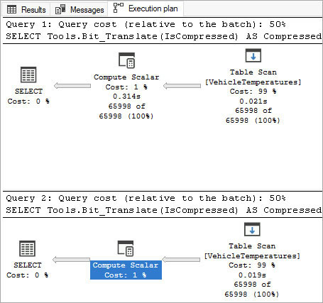
Figure 14-11 Query plan output for two runs, the first in SQL Server 2017 (14.0) compatibility level, and the second in SQL Server 2022 (16.0) benefitting from scalar UDF inlining.
The big thing to notice between these two executions is that the compute scalar in query 2 appears as a typical compute scalar operator, for any scalar expression not including a UDF. In query 1, it shows rows passing through, and an amount of time as it calculates the scalar for each row that passes through. Even in this extremely simple case, we saved time because we avoided running the function in a cursor-like loop for every row.
There are limitations to scalar UDF inlining, such as not working when time dependent intrinsic functions like SYSDATETIME() are present. You cannot change security context using EXECUTE AS (only EXECUTE AS CALLER, the default, is allowed). You also cannot benefit from scalar UDF inlining when referencing table variables or table-valued parameters.
- For more details and the complete list of requirements see https://learn.microsoft.com/sql/relational-databases/user-defined-functions/scalar-udf-inlining.
Scalar UDF inlining has immediate value for databases whose programmers have overused scalar UDFs. For many, scalar UDF inlining removes the problematic performance stigma associated with scalar UDFs, opening up more use cases. Formatting functions and translation functions where it might be easier than creating a table are now possible and will perform very well, as opposed to destroying your performance.