
Hearing Music in Different Environments
Chapter Contents
6.1 Acoustics of Enclosed Spaces
6.1.3 The effect of absorption on early reflections
6.1.5 The behavior of the reverberant sound field
6.1.6 The balance of reverberant to direct sound
6.1.7 The level of the reverberant sound in the steady state
6.1.8 Calculating the critical distance
6.1.9 The effect of source directivity on the reverberant sound
6.1.11 Calculating and predicting reverberation time
6.1.12 The effect of room size on reverberation time
6.1.13 The problem of short reverberation times
6.1.14 A simpler reverberation time equation
6.1.16 Reverberation time variation with frequency
6.1.17 Reverberation time calculation with mixed surfaces
6.1.18 Reverberation time design
6.1.19 Ideal reverberation time characteristics
6.1.22 Early reflections and performer support
6.1.23 The effect of air absorption
6.2 Room Modes and Standing Waves
6.2.4 A universal modal frequency equation
6.2.7 The decay time of axial modes
6.2.8 The decay time of other mode types
6.2.10 Acoustically “large” and “small” rooms
6.2.11 Calculating the critical frequency
6.4.3 Amplitude reflection gratings
6.5.1 Ways of achieving sound isolation
6.6 The Effect of Room Boundaries on Loudspeaker Output
6.7 Reduction of Enclosure Diffraction Effects
In this chapter we will examine the behavior of the sound in a room with particular reference to how the room’s characteristics affect the quality of the perceived sound. We will also examine strategies for analyzing and improving the acoustic quality of a room. Finally we will look at how rooms affect the output of loudspeakers.
6.1 Acoustics of Enclosed Spaces
In Chapter 1 the concept of a wave propagating without considering any boundaries was discussed. However, most music is listened to within a room, and is therefore influenced by the presence of boundaries, and so it is important to understand how sound propagates in such an enclosed space. Figure 6.1 shows an idealized room with a starting pistol and a listener; assume that at some time (t = 0) the gun is fired. There are three main aspects to how the sound of a gun behaves in the room, which are as follows.

Figure 6.1 An idealized room with an impulse excitation from a pistol.
6.1.1 The Direct Sound
After a short delay the listener in the space will hear the sound of the starting pistol, which will have traveled the shortest distance between it and the listener. The delay will be a function of the distance, as sound travels 344 meters (1129 feet) per second or approximately 1 foot per millisecond. The shortest path between the starting pistol and the listener is the direct path, and therefore this is the first thing the listener hears. This component of the sound is called the direct sound, and its propagation path and associated time response are shown in Figure 6.2.

Figure 6.2 The direct sound in a room.
The direct component is important because it carries the information in the signal in an uncontaminated form. Therefore a high level of direct sound is required for a clear sound and good intelligibility of speech. The direct sound also behaves in the same way as sound in free space, because it has not yet interacted with any boundaries. This means that we can use the equation for the intensity of a free space wave some distance from the source to calculate the intensity of the direct sound. The intensity of the direct sound is therefore given, from Chapter 1, by:
![]()
where Idirect sound = | the sound intensity (in W m–2) |
Q = | the directivity of the source (compared to a sphere) |
WSource = | the power of the source (in W) |
and r = | the distance from the source (in m) |
Equation 6.1 shows that the intensity of the direct sound reduces as the square of the distance from the source, in the same way as a sound in free space. This has important consequences for listening to sound in real spaces. Let us calculate the sound intensity of the direct sound from a loudspeaker.
A loudspeaker radiates a sound intensity level of 102 dB at 1 m. What is the sound intensity level (/direct) of the direct sound at a distance of 4 m from the loudspeaker?
The sound intensity of the direct sound at a given distance can be calculated, using Equation 1.18 from Chapter 1, as:
![]()
As we already know the intensity level at 1 m this equation becomes:
Idirect sound = I1m – 20 log10 (r)
which can be used to calculate the direct sound intensity as:
Idirect sound = 102 dB – 20 log10 (4) = 102 dB – 12dB = 90dB
Example 6.1 shows that the effect of distance on the direct sound intensity can be quite severe.
6.1.2 Early Reflections
A little time later the listener will then hear sounds which have been reflected off one or more surfaces (walls, floor, etc.), as shown in Figure 6.3. These sounds are called early reflections and they are separated in both time and direction from the direct sound. These sounds will vary as the source or the listener moves within the space. We use these changes to give us information about both the size of the space and the position of the source in the space. If any of these reflections are very delayed, i.e., total path length difference longer than about 30 milliseconds (33 feet), then they will be perceived as echoes. Early reflections can cause interference effects, as discussed in Chapter 1, and these can both reduce the intelligibility of speech and cause unwanted timbre changes in music in the space.

Figure 6.3 The early reflections in a room.
The intensity levels of the early reflections are affected by both the distance and the surface from which they are reflected. In general most surfaces absorb some of the sound energy and so the reflection is weakened by the absorption. However, it is possible to have surfaces which “focus” the sound, as shown in Figure 6.4, and in these circumstances the intensity level at the listener will be enhanced.
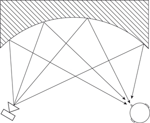
Figure 6.4 A focusing surface.
It is important to note, however, that the total power in the sound will have been reduced by the interaction with the surface. This means that there will be less sound intensity at other positions in the room. Also any focusing structure must be large when measured with respect to the sound wavelength, which tends to mean that these effects are more likely to happen for high-, rather than low-frequency components. In general therefore the level of direct reflections will be less than that which would be predicted by the inverse square law, due to surface absorption. Let us calculate the amplitude of an early reflection from a loudspeaker.
Example 6.2
A loudspeaker radiates a peak sound intensity of 102 dB at 1 m. What is the sound intensity level (/reflection), and delay relative to the direct sound, of an early reflection when the speaker is 1.5 m away from a hard reflecting wall and the listener is at a distance of 4 m in front of the loudspeaker?
The geometry of this arrangement is shown in Figure 6.5 and we can calculate the extra path length due to the reflection by considering the “image” of the loudspeaker, also shown in Figure 6.6, and by using Pythagoras’ theorem. This gives the path length as 5 m.

Figure 6.5 A geometry for calculating the intensity of an early reflection.

Figure 6.6 The maximum bounds for early reflections assuming no absorption or focusing.
Given the intensity level at 1 m, the intensity of the early reflection can be calculated because the reflected wave will also suffer from an inverse square law reduction in amplitude:
![]()
which can be used to calculate the direct sound intensity as:
Iearly reflection = 102dB – 20 log10(5) = 102dB – 14dB = 88dB
Comparing this with the earlier example we can see that the early reflection is 2 dB lower in intensity compared with the direct sound. The delay is simply calculated from the path length as:
![]()
Similarly the delay of the direct sound is:
![]()
So the early reflection arrives at the listener 14.5 ms – 11.6 ms = 2.9 ms after the direct sound.
Because there is a direct correspondence between delay, distance from the source, and the reduction in intensity due to the inverse square law, we can plot all this on a common graph (see Figure 6.6), which shows the maximum bounds of the intensity level of reflections, provided there are no focusing effects.
6.1.3 The Effect of Absorption on Early Reflections
How does the absorption of sound affect the level of early reflections heard by the listener? The absorption coefficient of a material defines the amount of energy, or power, that is removed from the sound when it strikes it. In general the absorption coefficient of real materials will vary with frequency, but for the moment we shall assume they do not. The amount of energy, or power, removed by a given area of absorbing material will depend on the energy, or power, per unit area striking it. As the sound intensity is a measure of the power per unit area this means that the intensity of the sound reflected is reduced in proportion to the absorption coefficient. That is:
![]()
where Intensityreflected = | the sound intensity reflected after absorption (in W m–2) |
Intensityincident = | the sound intensity before absorption (in W m–2) |
and α = | the absorption coefficient |
Because a multiplication of sound levels is equivalent to adding the decibels together, as shown in Chapter 1, Equation 6.3 can be expressed directly in terms of the decibels as:
![]()
which can be combined with Equation 6.2 to give a means of calculating the intensity of an early reflection from an absorbing surface:
![]()
As an example consider the effect of an absorbing surface on the level of the early reflection level calculated earlier.
A loudspeaker radiates a peak sound intensity of 102 dB at 1 m. What is the sound intensity level (/early reflection) of an early reflection, when the speaker is 1.5 m away from a reflecting wall and the listener is at a distance of 4 m in front of the loudspeaker, and the wall has an absorption of 0.9, 0.69, 0.5?
As we already know the Intensity level at 1 m, the Intensity of the early reflection can be calculated using Equation 6.5 because the reflected wave also suffers from an inverse square law reduction in amplitude:
![]()
The path length, from the earlier calculation, is 5 m so the sound intensity at the listener for the three different absorption coefficients is:

6.1.4 The Reverberant Sound
At an even later time the sound has been reflected many times and is arriving at the listener from all directions, as shown in Figure 6.7. Because there are so many possible reflection paths, each individual reflection is very close in time to its neighbors and thus there is a dense set of reflections arriving at the listener. This part of the sound is called reverberation and is desirable as it adds richness to, and supports, musical sounds. Reverberation also helps integrate all the sounds from an instrument so that a listener hears a sound which incorporates all the instruments’ sounds, including the directional parts. In fact we find rooms which have very little reverberation uncomfortable and generally do not like performing music in them; it is much more fun to sing in the bathroom compared with the living room (consider tracks 75–77 on the accompanying CD).

Figure 6.7 The reverberant sound in a room.
The time taken for reverberation to occur is a function of the size of the room and will be shorter for smaller rooms, due to the shorter time between reflections and the losses incurred on each impact with a surface. In fact the time gap between the direct sound and reverberation is an important cue to the size of the space that the music is being performed in. Because some of the sound is absorbed at each reflection it dies away eventually. The time that it takes for the sound to die away is called the reverberation time and is dependent on both the size of the space and the amount of sound absorbed at each reflection. In fact there are three aspects of the reverberant field that the space affects (see Figure 6.8).
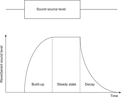
Figure 6.8 The time and amplitude evolution of the reverberant sound in a room.
- The increase of the reverberant field level: This is the initial portion of the reverberant field and is affected by the room size, which affects the time between reflections and therefore the time it takes the reverberant field to build-up. The amount of absorption in the room also affects the time that it takes the sound to get to its steady-state level. This is because, as shall be shown later, the steady-state level is inversely proportional to the amount of absorption in the room. As the rate at which sound builds up depends on the time between reflections and the absorption, the reverberant sound level will take more time to reach a louder level than reach a smaller one.
- The steady-state level of the reverberant field: If a steady tone, such as an organ note, is played in the space then after a period of time the reverberant sound will reach a constant level because at that point the sound power input balances the power lost by absorption in the space. This means that the steady-state level will be higher in rooms that have a small amount of absorption, compared with rooms that have a lot of absorption. Note that a transient sound in the space will not reach a steady-state level.
- The decay of the reverberant field level When a tone in the space stops, or after a transient, the reverberant sound level will not reduce immediately but will instead decay at a rate determined by the amount of sound energy that is absorbed at each reflection. Thus in spaces with a small amount of absorption the reverberant field will take longer to decay.
Bigger spaces tend to have longer reverberation times and well-furnished spaces tend to have shorter reverberation times. Reverberation time can vary from about 0.2 of a second for a small well-furnished living room to about 10 seconds for a large glass and stone cathedral.
6.1.5 The Behavior of the Reverberant Sound Field
The reverberation part of the sound in a room behaves differently compared with the direct sound and early reflections from the perspective of the listener. The direct sound and early reflections follow the inverse square law, with the addition of absorption effects in the case of early reflections, and so their amplitude varies with position. However, the reverberant part of the sound largely remains constant with the position of the listener in the room. This is not due to the sound waves behaving differently from normal waves; instead it is due to the fact that the reverberant sound waves arrive at the listener from all directions.
The result is that at any point in the room there are a large number of sound waves whose intensities are being added together. These sound waves have many different arrival times, directions and amplitudes because the sound waves are reflected back into the room, and so shuttle forward, backward and sideways around the room as they decay. The steady-state sound level, at a given point in the room, therefore is an integrated sum of all the sound intensities in the reverberant part of the sound, as shown in Figure 6.9. Because of this behavior the reverberant part of the sound in a room is often referred to as the “reverberant field.”

Figure 6.9 The source of the steady-state sound level of the reverberant field.
6.1.6 The Balance of Reverberant to Direct Sound
This behavior of the reverberant field has two consequences. Firstly, the balance between the direct and reverberant sounds will alter depending on the position of the listener relative to the source. This is due to the fact that the level of the reverberant field is independent of the position of the listener with respect to the source, whereas the direct sound level is dependent on the distance between the listener and the sound source. These effects are summarized in Figure 6.10, which shows the relative levels of direct to reverberant field as a function of distance from the source. This figure shows that there is a distance from the source at which the reverberant field will begin to dominate the direct field from the source. The transition occurs when the two are equal and this point is known as the “critical distance.”

Figure 6.10 The composite effect of direct sound and reverberant field on the sound intensity, as a function of the distance from the source.
6.1.7 The Level of the Reverberant Sound in the Steady State
Secondly, because in the steady state the reverberant sound at any time instant is the sum of all the energy in the reverberation tail, the overall sound level is increased by reverberation. The level of the reverberation will depend on how fast the sound is absorbed in the room. A low level of absorption will result in sound that stays around in the room for longer and so will give a higher level of reverberant field. In fact, if the average level of absorption coefficient for the room is given by a, the power level in the reverberant sound in a room can be calculated using the following equation:
![]()
the reverberant sound power (in W) | |
S = | the total surface area in the room (in m2) |
WSource = | the power of the source (in W) |
and α = | the average absorption coefficient in the room |
Equation 6.6 is based on the fact that, at equilibrium, the rate of energy removal from the room will equal the energy put into its reverberant sound field. As the sound is absorbed when it hits the surface, it is absorbed at a rate which is proportional to the surface area times the average absorption, or Sa. This is similar to a leaky bucket being filled with water where the ultimate water level will be that at which the water runs out at the same rate as it flows in (see Figure 6.11.)

Figure 6.11 The leaky bucket model of reverberant field intensity level.
The amount of sound energy available for contribution to the reverberant field is also a function of the absorption because if there is a large amount of absorption then there will be less direct sound reflected off a surface to contribute to the reverberant field—remember that before the first reflection the sound is direct sound. The amount of sound energy available to contribute to the reverberant field is therefore proportional to the residual energy left after the first reflection, or (1 – α) because α is absorbed at the first surface. The combination of these two effects gives (1 – α)/Sα—the term in Equation 6.6. The factor of four in Equation 6.6 arises from the fact that sound is approaching the surfaces in the room from all possible directions.
An interesting result from Equation 6.6 is that it appears that the level of the reverberant field depends only on the total absorbing surface area. In other words it is independent of the volume of the room. However, in practice the surface area and volume are related because one encloses the other. In fact, because the surface area in a room becomes less as its volume decreases, the reverberant sound level becomes higher for a given average absorption coefficient in smaller rooms although the reverberation time in the smaller room will always be shorter. Another way of visualizing this is to realize that in a smaller room there is less volume for a given amount of sound energy to spread out in, like a pat of butter on a smaller piece of toast. Therefore the energy density, and thus the sound level, must be higher in smaller rooms. However, there are more impacts per second with the surface of a smaller room, which gives rise to the more rapid decay than in a larger room.
The term (1 – α)/Sα in Equation 6.6 is often inverted to give a quantity known as the room constant, R, which is given by:
![]()
where R = | the room constant (in m2) |
and α = | the average absorpation coefficient in the room |
Using the room constant Equation 6.6 simply becomes:
![]()
In terms of the sound power level this can be expressed as:
![]()
As α is a number between 0 and 1 this also means that the level of the reverberant field will be greater in a room with a small surface area, compared with a larger room, for a given level of absorption coefficient. However, one must be careful in taking this result to extremes. A long and very thin cylinder will have a large surface area, but Equation 6.6 will not predict the reverberation level correctly because in this case the sound will not visit all the surfaces with equal probability. This will have the effect of modifying the average absorption coefficient and so will alter the prediction of Equation 6.6.
Therefore one must take note of an important assumption behind Equation 6.6 which is that the reverberant sound visits all surfaces with equal probability and from all possible directions. This is known as the “diffuse field assumption.” It can also be looked at as a definition of a diffuse field. In general the assumption of a diffuse field is reasonable and it is usually a design goal for most acoustics. However, it is important to recognize that there are situations in which it breaks down, for example at low frequencies.
As an example consider the effect of different levels of absorption and surface area on the level of the reverberant field that might arise from the loudspeaker described earlier.
Example 6.4
A loudspeaker radiates a peak sound intensity of 102 dB at 1 m. What is the sound pressure level of the reverberant field if the surface area of the room is 75 m2, and the average absorption coefficient is (a) 0.9 and (b) 0.2? What would be the effect of doubling the surface area in the room while keeping the average absorption the same?
From Equation 1.18 we can say:

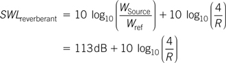
Thus the sound power level (SWL) radiated by the loudspeaker is:
![]()
The power in the reverberant field is given by:
![]()
The room constant “R” for the two cases is:
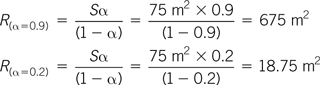
The level of the reverberant field can therefore be calculated from:
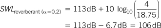
which gives:

and
The effect of doubling the surface area is to increase the room constant by the same proportion, so we can say that:
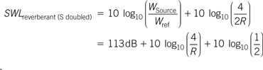
which gives:
![]()
Thus the effect of doubling the surface area is to reduce the level of the reverberant field by 3 dB in both cases.
Clearly the level of the reverberant field is strongly affected by the level of average absorption. The first example would be typical of an extremely “dead” acoustic environment, as found in some studios, whereas the second is typical of an average living room. The amount of loudspeaker energy required to produce a given volume in the room is clearly much greater, about 15 dB, in the first room compared with the second. If there is a musician in the room then they will experience a “lift” in output due to the reverberant field in the room. Because of this musicians feel uncomfortable playing in rooms with a low level of reverberant field and prefer performing in rooms which help them in producing more output. This is also one of the reasons we prefer singing in the bathroom. However, where the quality control of a recording is the goal, many recording engineers need much shorter room decay times because room reverberation can mask low-level detail.
6.1.8 Calculating the Critical Distance
The reverberant field is, in most cases, diffuse, and therefore visits all parts of the room with equal probability. Also at any point, and at any instant, we hear the total power in the reverberant field, as discussed earlier. Because of this it is possible to equate the power in the reverberant field to the sound pressure level. Thus we can say:
![]()
The distance at which the reverberant level equals the direct sound—the critical distance—can also be calculated using the above equations. At the critical distance the intensity due to the direct field and the power in the reverberant field at a given point are equal so we can equate Equation 6.1 and Equation 6.8 to give:

Which can be rearranged to give:
![]()
Thus the critical distance is given by:
![]()
Equation 6.11 shows that the critical distance is determined only by the room constant and the directivity of the sound source. Because the room constant is a function of the surface area of the room, the critical distance will tend to increase with larger rooms. However, many of us listen to music in our living rooms so let us calculate the critical distance for a hi-fi loudspeaker in a living room.
Example 6.5
What is the critical distance for a free-standing, omnidirectional, loudspeaker radiating into a room whose surface area is 75 m2, and whose average absorption coefficient is 0.2? What would be the effect of mounting the speaker into a wall?
The speaker is omnidirectional so the “Q” is equal to 1. The room constant “R” Is the same as was found in the earlier example, 18.75 m2. Substituting both these values into Equation 6.11 gives:
![]()
This is a very short distance! If the speaker is mounted in the wall the “Q” increases to 2, because the speaker can only radiate into 2 π steradians; so the critical distance increases to:
![]()
Which is still quite small!
As most people would be about 2 m away from their loudspeakers when they are listening to them this means that in a normal domestic setting the reverberant field is the most dominant source of sound energy from the hi-fi, and not the direct sound. Therefore the quality of the reverberant field is an important aspect of the performance of any system which reproduces recorded music in the home. There is also an effect on speech intelligibility in a reverberant space as the direct sound is the major component of the sound which provides this.
The level of the reverberant field is a function of the average absorption coefficient in the room. Most real materials, such as carpets, curtains, sofas and wood paneling have an absorption coefficient which changes with frequency. This means that the reverberant field level will also vary with frequency, in some cases quite strongly. Therefore in order to hear music, recorded or otherwise, with good fidelity, it is important to have a reverberant field which has an appropriate frequency response. As seen in the previous chapter, one of the cues for sound timbre is the spectral content of the sound which is being heard, and this means that when the reverberant field is dominant, as it is beyond the critical distance, it will determine the perceived timbre of the sound. This subject will be considered in more detail later in the chapter.
6.1.9 The Effect of Source Directivity on the Reverberant Sound
There is an additional effect on the reverberation field, and that is the directivity of the source of sound in the room. Most hi-fi loudspeakers, and musical instruments, are omnidirectional at low frequencies but are not necessarily so at higher ones. As the level of the reverberant field is a function of both the average absorption and the directivity of the source, the variation in directivity of real musical sources will also have an effect on the reverberant sound field and hence the perception of the timbre of the sound. Consider the following example of a typical domestic hi-fi speaker in the living room considered earlier.
Example 6.6
A hi-fi loudspeaker, with a flat-on axis, direct field, response, has a “Q” which varies from 1 to 25, and radiates a peak on axis sound intensity of 102 dB at 1 m. The surface area of the room is 75 m2, and the average absorption coefficient is 0.2. Over what range does the sound pressure level of the reverberant field vary?
As the speaker has a flat-on axis response the intensity of the direct field given by Equation 6.1 should be constant. That is:
![]()
where Idirective source = | the sound intensity (in W m–2) |
Q = | the directivity of the source (compared to a sphere) |
WSource = | the power of the source (in W) |
and r = | the distance from the source (in m) |
should be constant. Therefore the sound power radiated by the loudspeaker can be calculated by rearranging Equation 6.12 to give:
![]()
Equation 6.13 shows that in order to achieve a constant direct sound response the power radiated by the source must reduce as the “Q” increases. The power in the reverberant field is given by:
![]()
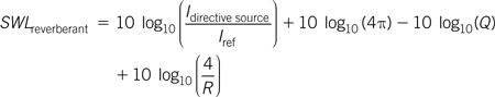
By combining Equations 6.13 and 6.14 the reverberant field due to the loudspeaker can be calculated as:
![]()
which gives a level for the reverberant field as:
The room constant “R” is 18.75 m2, as calculated in Example 6.4.
The level of the reverberant field can therefore be calculated as:

which gives:
![]()
for the level of the reverberant field when the “Q” is equal to 1, and:
![]()
when the “Q” is equal to 25.
Thus the reverberant field varies by 106.3 – 92.3 = 14 dB over the frequency range.
The effect therefore of a directive source with constant on-axis response is to reduce the reverberant field as the “Q” gets higher. The subjective effect of this would be similar to reducing the high “Q” regions via the use of a tone control, which would not normally be acceptable as a sound quality.
A typical reverberant response of a typical domestic hi-fi speaker is shown in Figure 6.12. Note that the reverberant response tends to drop in both the midrange and high frequencies. This is due to the bass and treble speakers becoming more directive at the high ends of their frequency range. The dip in reverberant energy will make the speaker less “present” and may make sounds in this region harder to hear in the mix. The drop in reverberant field at the top end will make the speaker sound “duller.” Some manufacturers try to compensate for these effects by allowing the on-axis response to rise in these regions; however, this brings other problems. The reduction in reverberant field with increasing “Q” is used to advantage in speech systems to raise the level of direct sound above the reverberant field and so improve the intelligibility.

Figure 6.12 The reverberant response of a domestic two-way high-fidelity loudspeaker.
However, in many professional recording studios’ control rooms, acoustic means are used to control the off-axis response irregularities and to cause a generally flat on-axis response, but such methods are often beyond the means of domestic listeners.
6.1.10 Reverberation Time
Another aspect of the reverberant field is that sound energy which enters it at a particular time dies away. This is because each time the sound interacts with a surface in the room it loses some of its energy due to absorption. The time that it takes for sound at a given time to die away in a room is called the reverberation time. Reverberation time is an important aspect of sound behavior in a room. If the sound dies away very quickly we perceive the room as being “dead” and we find that listening to, or producing, music within such a space is unrewarding. On the other hand when the sound dies away very slowly we perceive the room as being “live.” A live room is preferred to a dead room when it comes to listening to, or producing, live music. On the other hand when listening to recorded music, which already has reverberation as part of the recording, a dead room is often preferred.
However, as in many pleasurable aspects of life, reverberation must be taken in moderation. In fact the most appropriate length of reverberation time depends on the nature of the music being played. For example, fast pieces of contrapuntal music, like that of Scarlatti or Mozart, require a shorter reverberation time compared with large romantic works, like that of Wagner or Berlioz, to be enjoyed at their best. The most extreme reverberation times are often found in cathedrals, ice rinks, and railway stations and these acoustics can convert many musical events to “mush” yet to hear slow vocal polyphony, for example works by Palestrina, in a cathedral acoustic can be ravishing! This is because the composer has made use of the likely performance acoustic as part of the composition.
Because of the importance of reverberation time in the perception of music in a room, and because of the differing requirements for speech and different types of music, much effort is focused on it. In fact a major step in room acoustics occurred when Wallace Clement Sabine enumerated a means of calculating, and so predicting, the reverberation time of a room in 1898. Much design work on auditoria in the first half of this century focused almost exclusively on this one parameter, with some successes and some spectacular failures. Nowadays other acoustical and psychoacoustical factors are also taken into consideration.
6.1.11 Calculating and Predicting Reverberation Time
Clearly the length of time that it takes for sound to die is a function not only of the absorption of the surfaces in a room, but also of the length of time between interactions with the surfaces of the room. We can use these facts to derive an equation for the reverberation time in a room. The first thing to determine is the average length of time that a sound wave will travel between interactions with the surfaces of the room. This can be found from the mean free path of the room which is a measure of the average distances between surfaces, assuming all possible angles of incidence and position. For an approximately rectangular box the mean free path is given by the following equation:
![]()
where MFP = | the mean free path (in m) |
V = | the volume (in m3) |
and S = | the surface area (in m2) |
The time between surface interactions may be simply calculated from Equation 6.15 by dividing it by the speed of sound to give:
![]()
where τ = | the time between reflections (in s) |
and c = | the speed of sound (in ms–1) |
Equation 6.16 gives us the time between surface interactions and at each of these interactions α is the proportion of the energy absorbed, where α is the average absorption coefficient discussed earlier. If α of the energy absorbed at the surface then (1 – α) is the proportion of the energy reflected back to interact with further surfaces. At each surface a further proportion, α, of energy will be removed so the proportion of the original sound energy that is reflected will reduce exponentially. The combination of the time between reflections and the exponential decay of the sound energy, through progressive interactions with the surfaces of the room, can be used to derive an expression for the length of time that it would take for the initial energy to decay by a given ratio. (See Appendix 3 for details.)
There is an infinite number of possible ratios that could be used. However, the most commonly used ratio is that which corresponds to a decrease in sound energy of 60 dB, or 106. This gives an equation for the 60 dB reverberation time, known as T60, which is, from Appendix 4:
![]()
where T60 = the 60dB reverberation time (in s)
Equation 6.17 is known as the “Norris-Eyring reverberation formula;” the negative sign in the top compensates for the negative sign that results from the natural logarithm resulting in a reverberation time which is positive. Note that it is possible to calculate the reverberation time for other ratios of decay and that the only difference between these and Equation 6.17 would be the value of the constant. The argument behind the derivation of reverberation time is a statistical one and so there are some important assumptions behind Equation 6.17. These assumptions are:
- that the sound visits all surfaces with equal probability, and at all possible angles of incidence. That is, the sound field is diffuse. This is required in order to invoke the concept of an average absorption coefficient for the room. Note that this is a desirable acoustic goal for subjective reasons as well; we prefer to listen to and perform music in rooms with a diffuse field.
- that the concept of a mean free path is valid. Again this is required in order to have an average absorption coefficient, but in addition it means that the room’s shape must not be too extreme. This means that this analysis is not valid for rooms which resemble long tunnels. However, most real rooms are not too deviant and the mean free path equation is applicable.
6.1.12 The Effect of Room Size on Reverberation Time
The result in Equation 6.17 also allows some broad generalizations to be made about the effect of the size of the room on the reverberation time, irrespective of the quantity of absorption present. Equation 6.17 shows that the reverberation time is a function of the surface area, which determines the total amount of absorption, and the volume, which determines the mean time between reflections in conjunction with the surface area. Consider the effect of altering the linear dimensions of the room on its volume and surface area. These clearly vary in the following way:
V ∞ (Linear dimension)3
and
S ∞ (Linear dimension)2
However, both the mean time between reflections, and hence the reverberation time, vary as:
![]()
Hence as the room size increases the reverberation time increases proportionally, if the average absorption remains unaltered. In typical rooms the absorption is due to architectural features such as carpets, curtains and people, and so tends to be a constant fraction of the surface area. The net result is that, in general, large rooms have a longer reverberation time than smaller ones and this is one of the cues we use to ascertain the size of a space, in addition to the initial time delay gap. Thus one often hears people referring to the sound of a “big” or “large” acoustic as opposed to a “small” one when they are really referring to the reverberation time. Interestingly, now that it is possible to provide a long reverberation time in a small room, via electronic reverberation enhancement systems, with good quality, people have found that long reverberation times in a small room sound “wrong” because the visual cues contradict the audio ones. That is, the listener, on the basis of the apparent size of the space and their experience, expects a shorter reverberation time than they are hearing. Apparently closing one’s eyes restores the illusion by removing the distracting visual cue!
Let us use Equation 6.17 to calculate some reverberation times.
Example 6.7
What is the reverberation time of a room whose surface area is 75 m2, whose volume is 42 m3, and whose average absorption coefficient is 0.9, 0.2? What would be the effect of doubling all the dimensions of the room while keeping the average absorption coefficients the same?
Using Equation 6.17 and substituting in the above values gives, for α = 0.9:
![]()
which is very small! For α = 0.2 we get:
![]()
which would correspond well with the typical T60 of a living room, which is in fact what it is.
If the room dimensions are doubled then the ratio of volume with respect to the surface area also doubles so the new reverberation times are given by:
![]()
so the old reverberation times are increased by a factor of 2:
T60 doubled = T60 × 2
which gives a reverberation time of:
T60 doubled = T60 × 2 = 0.042 × 2 = 0.084 s
when α = 0.9 and:
T60 doubled = T60 – 2 = 0.043 × 2 = 0.086 s
when α = 0.2
6.1.13 The Problem of Short Reverberation Times
The very short reverberation times that occur when the absorption is high pose an interesting problem. Remember that one of the assumptions behind the derivation of the reverberation time calculation was that the sound energy visited all the surfaces in the room with equal probability. For our example room the mean time between reflections, using Equation 6.16, is given by:
![]()
If the reverberation time calculated in Example 6.7, when α = 0.9, is divided by the mean time between reflections then the average number of reflections that have occurred during the reverberation time can be calculated to be:
![]()
These are barely enough reflections to have hit each surface once! In this situation the reverberant field does not really exist; instead the decay of sound in the room is really a series of early reflections to which the concept of reverberant field or reverberation does not really apply. In order to have a reverberant field there must be much more than six reflections. A suitable number of reflections, in order to have a reverberant field, might be nearer 20, although this is clearly a hard boundary to accurately define. Many studios and control rooms have been treated so that they are very “dead” and so do not support a reverberant field.
6.1.14 A Simpler Reverberation Time Equation
Although the Norris–Eyring reverberation formula is often used to calculate reverberation times there is a simpler formula known as the “Sabine formula,” named after its developer Wallace Clement Sabine, which is also often used. Although it was originally developed from considerations of average energy loss from a volume, a derivation which involves solving a simple differential equation, it is possible to derive it from the Norris–Eyring reverberation formula. This also gives a useful insight into the contexts in which the Sabine formula can be reasonably applied. Consider the Norris–Eyring reverberation formula below:
![]()
The main difficulty in applying this formula is due to the need to take the natural logarithm of (1 − α). However, the natural logarithm can be expanded as an infinite series to give:
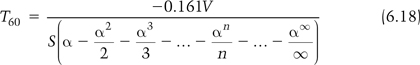
Because α < 1 the sequence always converges. However, if α < 0.3 then the error due to all the terms greater than −α is less than 5.7%. This means that Equation 6.18 can be approximated as:
![]()
Equation 6.19 is known as the “Sabine reverberation formula” and, apart from being useful, was the first reverberation formula. It was developed on the basis of experimental measurements made by W. C. Sabine, thus initiating the whole science of architectural acoustics. Equation 6.19 is much easier to use and gives accurate enough results provided the absorption, α, is less than about 0.3. In many real rooms this is a reasonable assumption. However, it becomes increasingly inaccurate as the average absorption increases and in the limit predicts a reverberation time when α = 1, that is reverberation without walls!
6.1.15 Reverberation Faults
As stated previously, the basic assumption behind these equations is that the reverberant field is statistically random, that is, a diffuse field. There are, however, acoustic situations in which this is not the case. Figure 6.13 shows the decay of energy, in dB, as a function of time for an ideal diffuse field reverberation. In this case the decay is a smooth straight line representing an exponential decay of an equal number of dBs per second.

Figure 6.13 The ideal decay versus time curve for diffuse field reverberation.
Figure 6.14 on the other hand shows two situations in which the reverberant field is no longer diffuse. In the first situation all the absorption is only on two surfaces, for example an office with acoustic tiles on the ceiling, carpets on the floor, and nothing on the walls. Here the sound between the absorbing surfaces decays quickly whereas the sound between the walls decays much more slowly, due to the lower absorption. In the second case there are two connected spaces, such as the transept and nave in a church, or under the balconies in a concert hall. In this case the sound energy does not couple entirely between the two spaces and so they will decay at different rates that depend on the level of absorption in them. In both of these cases the result is a sound energy curve as a function of time which has two or more slopes, as shown in Figure 6.15. This curve arises because the faster decaying waves die away before the more slowly decaying ones and so allow them to dominate in the end.

Figure 6.14 Two situations which give poor reverberation decay curves (see text).
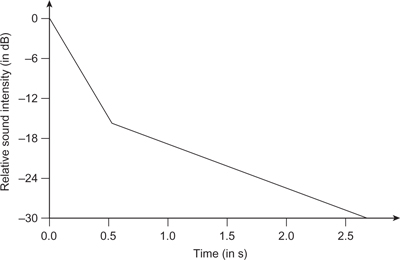
Figure 6.15 A double slope reverberation decay curve.
The second major acoustical defect in reverberant decay occurs when there are two precisely parallel and smooth surfaces, as shown in Figure 6.16. This results in a series of rapidly spaced echoes, onomatopoeically called flutter echoes, which result as the energy shuttles backward and forward between the two surfaces. These are most easily detected by clapping one’s hands between the parallel surfaces to provide the packet of sound energy to excite the flutter echo. The decay of energy versus time in this situation is shown in Figure 6.17 and the presence of the flutter echo manifests itself as a series of peaks in the decay curve. Note that this behavior is also often associated with the double-slope decay characteristic shown in Figure 6.15 because the energy shuttling between the parallel surfaces suffers less absorption compared with a diffuse sound.
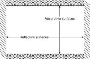
Figure 6.16 A situation which can cause flutter.

Figure 6.17 The decay versus time curve for flutter
6.1.16 Reverberation Time Variation with Frequency
Equations 6.17 and 6.18 show that the reverberation time depends on the volume, surface area, and the average absorption coefficient in the room. However, the absorption coefficients of real materials are not constant with frequency. This means that, assuming that the room’s volume and surface area are constant with frequency, which is not an unreasonable assumption, the reverberation time in the room will also vary with frequency. This will subjectively alter the timbre of the sound in the room due to both the effect on the level of the reverberant field discussed earlier and the change in timbre as the sound in the room decays away.
As an extreme example, if a particular frequency has a much slower rate of decay compared with other frequencies, then, as the sound decays away, this frequency will ultimately dominate and the room will “ring” at that particular frequency. The sound power for steady-state sounds will also have a strong peak at that frequency because of the effect on the reverberant field level.
Table 6.1 shows some typical absorption coefficients for some typical materials which are used in rooms as a function of frequency. Note that they are measured over octave bands. One could argue that third octave band measurements would be more appropriate psychoacoustically as the octave measurement will tend to blur variations within the octave, which might be perceptually noticeable. In many cases, because the absorption coefficient varies smoothly with frequency, octave measurements are sufficient. However, especially when considering resonant structures, more resolution would be helpful. Note also that there are often no measurements of the absorption coefficients below 125 Hz. This is due to both the difficulty in making such measurements and the fact that below 125 Hz other factors in the room become more important, as we shall see later.
Table 6.1 Typical absorption coefficients as a function of frequency for various materials

In order to take account of the frequency variation of the absorption coefficients we must modify the equations used to calculate the reverberation time as follows:
![]()
where α(f) = frequency-dependent absorption coefficient for the Norris–Eyring reverberation time equation and:
![]()
for the Sabine reverberation time equation.
6.1.17 Reverberation Time Calculation with Mixed Surfaces
In real rooms we must also allow for the presence of a variety of different materials, as well as accounting for their variation of absorption as a function of frequency. This is complicated by the fact that there will be different areas of material, with different absorption coefficients, and these will have to be combined in a way that accurately reflects their relative contribution. For example, a large area of a material with a low value of absorption coefficient may well have more influence than a small area of material with more absorption.
In the Sabine equation this is easily done by multiplying the absorption coefficient of the material by its total area and then adding up the contributions from all the surfaces in the room. These resulted in a figure which Sabine called the “equivalent open window area”, as he assumed, and experimentally verified, that the absorption coefficient of an open window was equal to 1.
The denominator in the Sabine reverberation equation, Equation 6.19, is also equivalent to the open window area of the room, but has been calculated using the average absorption coefficient in the room. It is therefore easy to incorporate the effects of different materials by simply calculating the total open window area for different materials, using the method described above, and substituting it for Sα in Equation 6.19. This gives a modified equation which allows for a variety of frequency-dependent materials in the room as:

where αi(f) = | absorption coefficient for a given material |
and Si = | its area |
For the Norris–Eyring reverberation time equation the situation is a little more complicated because the equation does not use the open window area directly. However, the Norris–Eyring reverberation time equation can be rewritten in a modified form, as shown in Appendix 4, which allows for the variation in material absorption due to both nature and frequency, as:

Equation 6.21 is also known as the “Millington-Sette equation.” Although Equation 6.21 can be used irrespective of the absorption level it is still more complicated than the Sabine equation and, if the average absorption coefficient is less than 0.3, it can be approximated very effectively by it, as discussed previously. Thus in many contexts the Sabine equation, Equation 6.20, is preferred.
Equation 6.20 is readily used in conjunction with tables of absorption coefficients to calculate the reverberation time and can be easily programmed into a spreadsheet. As an example, consider the reverberation time calculation for a living room outlined in Example 6.8.
Example 6.8
What is the 60 dB reverberation time (T60) of a living room as a function of frequency whose surface area is 75 m2 and whose volume is 42 m3? The floor is carpet on concrete, the ceiling is plaster on lath, and both have an area of 16.8 m2. There are 6 m2 of windows and the rest of the surfaces are painted plaster on brick; ignore the effect of the door.
Using the data in Table 6.1, set up a spreadsheet or table, as shown in Table 6.2, and calculate the equivalent open window area for each surface as a function of frequency. Having done that add up the individual surface contributions for each frequency band and apply Equation 6.20 to the result in order to calculate the reverberation time.
Table 6.2 Absorption and reverberation time calculations for an untreated living room

From the results shown in Table 6.2, which are also plotted in Figure 6.18, one can see that the reverberation varies from 1.49 seconds at low frequencies to 0.55 seconds at high frequencies. This is a normal result for such a structure and would tend to sound a bit “woolly” or “boomy.” The relative level of reverberant field for this room is also shown in Figure 6.19 and this shows approximately a 5 dB increase in the reverberant field at low frequencies.
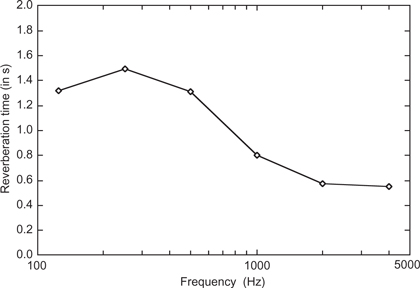
Figure 6.18 The reverberation time for the untreated room as a function of frequency.

Figure 6.19 The reverberation field level for the untreated room as a function of frequency.
6.1.18 Reverberation Time Design
The results of Example 6.8 beg the question: “How can we improve the evenness of the reverberation time?” The answer is to either add, or remove, additional absorbing materials into or from the room in order to achieve the desired reverberation characteristic. Here the concept of an open window area budget is useful. The idea is that, given the volume of the room, and the desired reverberation time, the necessary open window area required is calculated. The open window area already present in the room is then examined and, depending on whether the room is over or under budget, appropriate materials are added or removed. Consider Example 6.9 which tries to improve the reverberation of the previous room.
Example 6.9
Which single material could be added to the room in Example 6.8 which would result in an improved reverberation time, and what amount would be required to effect the improvement?
A material which has a high absorption at low frequencies, such as wood paneling, needs to be added to the room. If the absorption budget is set as being equivalent to the open window area at 4 kHz then we must achieve an open window area of 12.5 m over the whole frequency range. The worst frequency in the previous example is 250 Hz, which only has 4.5 m of open window area at that frequency. This means that any additional absorber must add 12.5 − 4.5 = 8 m of open window area at that frequency. The absorption of wood paneling, from Table 6.1, at 250 Hz is 0.25. Therefore the amount of wood paneling required is:
![]()
Table 6.3, Figure 6.20 and Figure 6.21 show the effect of applying the treatment, which dramatically improves the reverberation time characteristics. The reverberation time now only varies from 0.59 to 0.41 s, which is a much smaller variation than before. The peak-to-peak variation in the level of the reverberant field has also been reduced to less than 2 dB.
Table 6.3 Absorption and reverberation time calculations for a treated living room


Figure 6.20 The reverberation time for the treated room as a function of frequency.

Figure 6.21 The reverberation field level for the treated room as a function of frequency.
However, the overall reverberation time has gone down, especially at the lowest frequencies, because of the effect of the wood paneling at frequencies other than the one being concentrated on. Thus in practice an iterative approach to deciding on the most suitable treatment for a room is often required. Another point to consider is that the treatment proposed only just fits in the room, and sometimes it proves impossible to achieve a desired reverberation characteristic due to physical limitations.
6.1.19 Ideal Reverberation Time Characteristics
What is an ideal reverberation characteristic? We have seen that the decay should be a smooth exponential of a constant number of decibels of decay per unit time. We also know that different sorts of music require different reverberation times. In many cases the answer is: “it depends on the situation.” However, there are a few general rules which seem to be broadly accepted.
Firstly, there is a range of reverberation times which are a function of the type of music being played; music with a high degree of articulation needs a drier acoustic than music which is slower and more harmonic. Secondly, as the performance space gets larger the reverberation time required for all types of music becomes longer. This result is summarized in Figure 6.22 which shows the “ideal” reverberation time as a function of both music and room volume. Thirdly, in general, listeners prefer a rise in reverberation time in the bass (125 Hz) of about 40% relative to the midrange (1 kHz) value as shown in Figure 6.23. This rise in bass reverberation adds “warmth” and it also helps increase the sound level of bass instruments, which often have weak fundamentals, by raising the level of the reverberant field at low frequencies. However, when recording musical instruments, or when listening to recorded music, this bass lift due to the reverberant field may be undesirable and therefore a flat reverberation characteristic is preferred.

Figure 6.22 Ideal reverberation times as a function of room volume and musical style.

Figure 6.23 The ideal reverberation time versus frequency curves.
There are many other aspects of reverberation, too numerous to mention here, which must be considered when designing acoustic spaces. However, there are four aspects that are worthy of mention as they have proved to be the downfall of more than one acoustic designer, or manufacturer, of reverberation units.
6.1.20 Early Decay Time
The first aspect is that the measure of reverberation time as being the time it takes the sound to fall by 60 dB is not particularly relevant psychoacoustically; it is also very difficult to measure in situ. This is due to the presence of background noise, either unwanted or the music being played, which often results in less than 60 dB of energy decay before the decay sound becomes less than the residual noise in the environment. Even in the quieter environment of a Victorian town in the days before road traffic, Sabine had to do measurements, using his ears, at night to avoid the results being affected by the level of background noise. Because we rarely hear a full reverberant decay, our ears and brains have adapted, quite logically, to focus on what can be heard. Thus we are more sensitive to the effects of the first 20 to 30 dB of the reverberant decay curve.
In principle, provided we have an even exponential decay curve, the 60 dB reverberation is directly proportional to the earlier curves and so this should not cause any problems. However, if the curve is of the double-slope form shown in Figure 6.15 then this simple relationship is broken. The net result is that, although the T60 reverberation time may be an appropriate value, because of the faster early decay to below 30 dB we perceive the reverberation as being shorter than it really is. The psychoacoustic effect of this is that the space sounds “drier” than one would expect from a simple measurement of T60. Modern acoustic designers therefore worry much more about the early decay time (EDT) than they used to when designing concert halls.
6.1.21 Lateral Reflections
The second factor which has been found to be important for the listener is the presence of dense diffuse reflections from the side walls of a concert hall, called lateral reflections, as shown in Figure 6.24. The effect of these is to envelop or bathe the listener in sound and this has been found to be necessary for the listener to experience maximum enjoyment from the sound. It is important that these reflections be diffuse, as specular reflections will result in disturbing comb filter effects, as discussed in Chapter 1, and distracting images of the sound sources in unwanted and unusual directions. Providing diffuse reflections is thus important and this has been recognized for some time. Traditionally, plaster mouldings, niches and other decorative surface irregularities have been used to provide diffusion in an ad hoc manner. More recently diffusion structures based on patterns of wells whose depths are formally defined by an appropriate mathematical sequence have been proposed and used.

Figure 6.24 Lateral reflections in a concert hall.
However, it is not just the provision of diffusion on the side walls that must be considered. The traditional concert hall is called a shoebox hall, because of its shape, as shown in Figure 6.25, and this naturally provides a large number of lateral reflections to the audience. This shape, combined with the Victorian penchant for florid plaster decoration, resulted in some excellent sounding spaces. Unfortunately shoebox halls are harder to make a profit with because they cannot seat as many people as some other structures.

Figure 6.25 Lateral reflections in a shoebox concert hall.
Another popular structure, which has a different behavior as regards to lateral reflections, is the fan-shaped hall shown in Figure 6.26. This structure has the advantage of being able to seat more people with good sightlines but unfortunately it directs the lateral reflections away from the audience and those few that do arrive are very weak at the wider part of the fan. The situation can be improved via the use of explicit diffusion structures on the walls, ceilings, and mid-air as floating shapes, as shown in Figure 6.27. However, it has been found that the pseudo-lateral diffuse reflections from the ceiling are not quite comparable in effect to reflections from the side walls, and so the provision of a good listening environment within the realities of economics is still a challenge.

Figure 6.26 Lateral reflections in a fanshaped concert hall.

Figure 6.27 Lateral reflections from ceiling diffusion in a concert hall.
6.1.22 Early Reflections and Performer Support
A third factor, which is often ignored, is the acoustics that the performers experience. Pop groups have known about this for years and take elaborate precautions to provide each performer on stage with their own individual balance of acoustic sounds via a technique known as “foldback.” In fact some performers now receive their foldback directly into their ears via a technique known as “in-ear monitoring” and in many large gigs the equipment providing foldback to the performer can rival, or even exceed, that which provides the sound for the audience. The classical musician, however, only has the acoustics of the hall to provide them with “foldback.” Thus the musicians on the stage must rely on reflections from the nearby surfaces to provide them with the necessary sounds to enable them to hear themselves and each other.
There are two requirements for the sound reaching the performer on stage. It must be at a sufficient level, and arrive soon enough to be useful. To begin with it is important that the surfaces surrounding the performers direct some sound back to them. Note that there is a conflict between this and providing a maximum amount of sound to the audience so some compromise must be reached. The usual compromise is to make use of the sound which radiates behind the performers and direct it out to the audience via the performers, as shown in Figure 6.28. This has the twofold advantage of providing the performers with acoustic foldback and redirecting sound energy that might have been lost back to the audience. Ideally the sound that is redirected back to the performers should be diffuse as this will blend the sounds of the different instruments together for all the performers, as shown in Figure 6.29, whereas specular reflectors can have hot and cold spots for a given instrument on the stage.

Figure 6.28 Early reflections to provide acoustic foldback for the performer.

Figure 6.29 The effect of diffusion on the acoustic foldback for the performer.
An important aspect of acoustic foldback, however, is the time that it takes to arrive back at the performers. Ideally it should arrive immediately, and some does via the floor and direct sound from the instrument. However, the majority will have to travel to a reflecting or diffusing surface and back to the performers. There is evidence to show that, in order to maintain good ensemble comfortably, the musicians should receive the sound from other musicians within about 20 ms of the sound being produced. This means that ideally there should be a reflecting or diffusing surface within 10 ms (3.44 m or 11.5 ft) of the performer; the time is divided by 2 to allow for going to the reflecting surface and back. In practice some of the surfaces may have to be further away when large orchestral forces are being mustered, although the staging used can assist the provision of acoustic foldback. Sometimes, however, the orchestra enclosure is so large that the reflections arrive later than this. If they arrive later than about 50 ms the musicians will perceive them as echoes and ignore them. On the other hand if these reflections arrive at the boundary between perceiving it as part of the sound or an echo of a previous sound it can cause severe disruption of the performers’ perception of it.
The net effect of these “late early reflections” is to damage the performers’ ability to hear other instruments close to them, and this further reduces their ability to maintain ensemble. In one prestigious hall, the reason musicians used to complain that they couldn’t hear each other, and so hated playing there, was traced to the problem of late early reflections. As a postscript it is interesting to note that the orchestra enclosure in shoebox halls often did the right things. However, in modern multipurpose facilities it is often a challenge to provide the necessary acoustic foldback while allowing space for scenery and machinery, etc.
6.1.23 The Effect of Air Absorption
The fourth aspect of reverberation, which caught early reverberation unit designers by surprise, is the observation that, as well as suffering many reflections, the sound energy in a reverberant decay will have traveled through a lot of air. In fact the distance that the sound will have traveled will be directly proportional to the reverberation time, so a one second reverberation time implies that the sound will have traveled 344 m by the end of the decay. Although for low frequencies air absorbs a minimal amount of sound energy, at high frequencies this is not the case. In particular, humidity, smoke particles and other impurities will absorb high-frequency energy and so reduce the level of high frequencies in the sound. This is one of the reasons why people sound duller when they are speaking at a distance.
In terms of reverberation time, and also the level of the reverberant field, the effect of this extra absorption is to reduce the reverberation time, and the level of the reverberant field, at high frequencies. Fortunately this effect only becomes dominant at higher frequencies, above 2 kHz. Unfortunately, though, it is dependent on the level of humidity and smoke in the venue and so the high-frequency reverberation time, and the reverberant field level, will change as the audience stays in the space. Note this is an additional dynamic effect over and above the static absorption simply due to the presence of a clothed person in a space and is due to the fact that people exhale water vapor and perspire. Clearly then the degree of change will be a function of both the physical exertions of the audience and the quality of the ventilation system!
As the effect of air absorption is determined by the distance the sound has traveled, rather than its interaction with a surface, it is difficult to incorporate the effect into the reverberation time equations discussed earlier. An approximation that seems to work is to convert the effect of the air absorption into an equivalent absorption area by scaling an air absorption coefficient by the volume of the space. This is reasonable because as the volume of the room increases, the more air the wave must travel through and the longer the distance that it travels. This coefficient is shown at the bottom of Table 6.1 and from it one can see that for small rooms the effect can be ignored because until the volume becomes greater than 40 m3 the equivalent absorbing area is less than 1 m2. However, the effect does become significant if one is designing artificial reverberation units because, if it is not allowed for, the result will be an overbright reverberation, which sounds unnatural.
In this section the concept of reverberation time and reverberant field has been discussed. The assumption behind the equations has been that the sound field is diffuse. However, if this is not the case then the equations are invalid. Although at mid and high audio frequencies a diffuse field might be possible, either by accident or design, at low frequencies this is not the case due to the effect of the room’s boundaries causing standing waves.
6.2 Room Modes and Standing Waves
When a room is excited by an impulse, the sound energy is reflected from its surfaces. At each reflection some of the sound is absorbed and therefore the sound energy decays exponentially. Ideally the sound should be reflected from each surface with equal probability, forming a diffuse field. This results in a single exponential decay with a time constant proportional to the average absorption in the room. However, in practice not all the energy is reflected in a random fashion. Instead some energy is reflected in cyclic paths, as shown in Figure 6.30. If the length of the path is a precise number of half wavelengths then they will form standing waves in the room. These standing waves (resonant modes) have pressure and velocity distributions which are spatially static and so behave differently from the rest of the sound in the room in the following ways:

Figure 6.30 Cyclic reflection paths in a room
- They do not visit each surface with equal probability. Instead a subset of the surfaces is involved.
- They do not strike these surfaces with random incidence. Instead a particular angle of incidence is involved in the reflection of the standing wave.
- They require a coherent return of energy back to an original surface: a cyclic path. This is of necessity strongly frequency dependent and so these paths only exist for discrete frequencies which are determined by the room geometry.
Another name for these standing waves in a room are resonant modes and the frequencies at which they occur are known as “modal frequencies.” Because the modes are spatially static there will be a strong variation of sound pressure level as one moves around the room, which is undesirable. There are three basic types of room mode, which are outlined in Sections 6.2.1 to 6.2.3.
6.2.1 Axial modes
These modes occur between two opposing surfaces, as shown in Figure 6.31, and so are a function of the linear dimensions of the room. The frequencies of an axial mode are given by the following equation:

Figure 6.31 Axial modal paths in a room.
![]()
where fx(axial) = | the axial mode frequencies (in Hz) |
x = | the number of half wavelengths that fit between the surfaces (1, 2, …, ∞) |
L = | the distance between the reflecting surfaces (in m) |
and c = | the speed of sound (in ms–1) |
This equation shows that there are an infinite number of possible modal frequencies at which an integer number of wavelengths fit into the room, with lowest modal frequency occurring when just one half wavelength fits into the space between the reflecting surfaces.
6.2.2 Tangential Modes
These modes occur between four surfaces, as shown in Figure 6.32, and so are a function of two of the dimensions of the room. The frequencies of the tangential modes are given by the following equation:
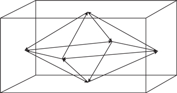
Figure 6.32 Tangential modal paths in a room.

where fxy(tangential) = | the tangential modal frequencies (in Hz) |
x = | the number of half wavelengths between one set of two surfaces (1, 2, …, ∞) |
y = | the number of half wavelengths between the other set of two surfaces (1, 2, …, ∞) |
and L, W = | the distance between the reflecting surfaces (in m) |
There is also an infinite number of tangential modes, but they must fit an integral number of half wavelengths in two dimensions. This has the interesting consequence that the lowest modal frequencies are higher than the axial modes, despite the fact that the apparent path length is greater. The reason is that the standing waves must fit between the opposing surfaces, that is, on the sides rather than the hypotenuse of the triangular path, and as the propagating wave travels down the hypotenuse, the effective wavelength, or phase velocity, on the sides of the room is larger, as shown in Figure 6.33. The lowest modal frequency for a tangential mode occurs when precisely one half wavelength, at the phase velocity, fits into each dimension.

Figure 6.33 The phase velocity of tangential room modes.
6.2.3 Oblique Modes
These modes occur between all six surfaces, as shown in Figure 6.34, and so are a function of all three dimensions of the room. The frequencies of the oblique modes are given by the following equation:
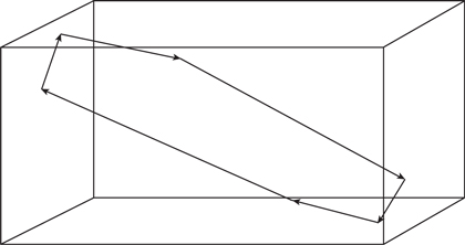
Figure 6.34 An oblique modal path in a room.
![]()
where fxyz(oblique) = | the oblique modal frequencies (in Hz) |
x, y, z = | the number of half wavelengths between the surfaces (1, 2, …, ∞) |
and L, W, H = | the distance between the reflecting surfaces (in m) |
The lowest frequencies of these modes are also higher than the lowest axial modes, for the reasons discussed earlier.
6.2.4 A Universal Modal Frequency Equation
The combination of these three types of mode forms a dense set of possible standing wave frequencies in the room and they can be combined into one equation by simply allowing x, y, and z in the oblique mode equation to range from 0, 1, 2 to infinity, giving the following equation which will give the frequencies of all possible modes in the room:
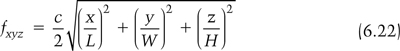
where x, y, z = | the number of half wavelengths between the surfaces (0, 1, 2, …, ∞) |
The above equation also shows that if any of the dimensions are integer multiples of each other then some of the modal frequencies will be the same, which can cause problems. It is therefore better to choose noncommensurate ratios for the wall dimensions to ensure that the modes are spread out as much as possible. Much work has been done on ideal room ratios and one set of favorable room dimensions is shown in Table 6.4. However, these dimensions are not necessarily the only optimum ones for all room sizes. It is also important to realize that room modes are inherent in any structure which encloses the sound sources. This means that changing the shape of the room, for example by angling the walls, does not remove the resonances—it merely changes their frequencies from values that are easily calculated to ones which are not. Both Walker (1996) and Cox et al. (2004) discuss more general and useful approaches to optimum room dimensions.
Table 6.4 Some favorable room dimensions

In general the number of resonances within a given frequency bandwidth increases with frequency. In fact it can be shown that they increase proportionally to the square of the frequency, and in large well-behaved acoustical spaces, which sound good, this increase in mode density with frequency is smooth. This is the rationale behind a method for assessing the modal behavior in a room known as the “Bonello criteria.” These criteria try to ascertain how significant the modal behavior of a room is in perceptual terms. This is done by dividing the audio frequency spectrum into third octave bands, as an approximation of critical bands, and then counting the number of modes per band. If the number of modes per third octave band increases monotonically then there is a good chance that we will perceive the room as having a “smooth” frequency response despite the resonances. If the number of resonances per third octave drops as the frequency rises then there will be a perceptually noticeable peak in the frequency response.
Coincident modes are also another way of creating a perceptually noticeable frequency response peak and the Bonello criteria do further stipulate that there should be no modal coincidence within a third octave band unless there are at least three additional non-coincident resonances to balance the two that are coincident. As an example of the calculation of mode frequencies let us calculate some for a typical living room.
Example 6.10
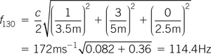
Calculate the lowest frequency mode in a room which measures 3.5 m × 5 m × 2.5 m. At what frequency would a tangential mode with one half wavelength along the 3.5 m dimension and three half wavelengths along the 5 m dimension occur, at what frequency would the (2 2 2) oblique mode occur, and at what frequency is the first coincident mode?
Using Equation 6.21 calculate the modes as follows. The lowest frequency mode is the first axial mode along the longest dimension of the room, which is the (0 1 0) or axial mode in this example, so the lowest modal frequency in the room is:

The mode with one half wavelength along the 3.5 m dimension and three half wavelengths along the 5 m dimension is the (1 3 0) or tangential mode so its frequency is:
The frequency of the (2 2 2) or oblique mode is:

The dimensions of 2.5 m and 5 m are related by a factor of 2 so the second axial mode along the 5 m dimension will be at the same frequency as the first axial mode along the 2.5 m dimension. That is:
f020 = f001
The (0 2 0) mode has a frequency of:

and (0 0 1) mode has a frequency
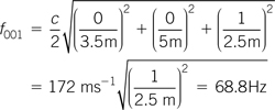
which are both at the same frequency and are therefore coincident.
As has been already discussed, modes behave differently to diffuse sound and this has the following consequences:
- The modes are not absorbed as strongly as sound which visits all surfaces. This is due to both the reduction in the number of surfaces visited and the change in absorption due to non-random incidence.
- This reduction in absorption is strongly frequency dependent and results in less absorption and therefore a longer decay time at the frequencies at which standing waves occur.
- The decay of sound energy in the room is no longer a single exponential decay with a time constant proportional to the average absorption in the room. Instead there are several decay times. The shortest one tends to be due to the diffuse sound field whereas the longer ones tend to be due to the resonant modes in the room. This results in excess energy at those frequencies with the attendant degradation of the sound in the room.
How does the energy in a mode decay as a function of time, how can it be related to the reverberation, and what is the effect of absorption in a mode on the frequency response?
6.2.7 The Decay Time of Axial Modes
The decay of sound energy in modes is in many respects identical to the decay of sound energy which is analyzed in Appendix 4. The main difference is that the absorption coefficient is sometimes smaller, because the modal sound wave does not have random incidence; it will also be specific to the surfaces involved instead of being an average value for the whole room. In addition the time between reflections will be dependent on the length of the modal path rather than the mean free path. This means that the decay time for a mode is likely to be different to the diffuse sound.
For example the length of an axial mode path is determined by the distance between the two reflecting surfaces that support the mode, which will be one of the room’s dimensions. Thus for an axial mode the energy left after a given time period is given by modifying Equation A4.5 in Appendix 4 using the distance between the surfaces instead of the mean free path to give:
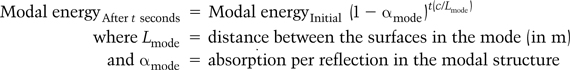
The above equation can be manipulated to give a 60 dB decay time, analogous to Equation 6.17, which is:

This expresses a similar result to Equation 6.17 except for the difference caused by the differing length of the modal structure with respect to the mean free path. If the length of the modal structure is longer than the mean free path then, assuming similar levels of absorption, the decay time for the mode will be longer than the diffuse field whereas if the length is smaller then the modal decay will be shorter than the diffuse field. The length between reflections is both a function of the surfaces that support the mode and the type of mode—axial, tangential, or oblique—that occurs. For axial modes the mode length, Lmode, is simply the relevant room dimension.
6.2.8 The Decay Time of other Mode Types
For the other types of mode the situation is more complicated, as shown in Figure 6.35 for a tangential mode. However, one could argue that the path length for this type of mode is given by the length of the hypotenuse of the triangle formed by half the length and half the width of the four walls that support the mode. That is, the modal length is given by:

Figure 6.35 The path length for a tangential mode.
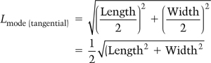
This equation shows that the distance between reflections for a tangential mode is essentially the diagonal dimension between the four surfaces that support the mode divided by two to allow for the fact that the wave suffers two reflections along this path. The length so derived can then be used as the modal length in the equation for the modal decay. A similar argument can be applied to the oblique modes, which visit all six surfaces. Because of this the modal supporting structure is a cuboid and the diagonal between opposing corners must be used. In addition the wave will suffer three relections along this path. This gives a path length for the oblique mode as:

The absorption does more than cause the mode to decay; it reduces the total energy stored in the mode, in a similar manner to the effect of absorption on the reverberant field, and also causes the mode to have a finite bandwidth which is proportional to the amount of absorption, as shown in Figure 6.36. The absorption also reduces the peak to minimum variation in the standing wave pattern, and so reduces the spatial variation of the sound pressure, as shown in Figure 6.37. The bandwidth of a mode can be calculated from the 60 dB decay time using the following equation:
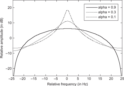
Figure 6.36 The bandwidth of modes for a given value of absorption.
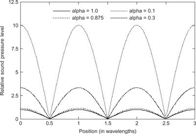
Figure 6.37 The spatial variation in the amplitude of modes for a given value of absorption.
![]()
where Bwmode = | the – 3dB bandwidth of the mode (in Hz) |
Because it is not always possible to calculate the true modal decay time this equation can be dangerously approximated using the reverberation time of the room as:
![]()
This assumption is dangerous because the mode will not be diffuse whereas the reverberation time calculation assumes a diffuse sound field. In general the bandwidths and intensity levels of a mode are proportional to the number of reflections required to support them. This means that axial modes tend to be the strongest followed by tangential and then oblique modes in order of strength, as shown in Figure 6.38. However, this is not always the case as a tangential mode in a room with four reflecting surfaces could be stronger than the axial mode between the other two absorbing surfaces.

Figure 6.38 Typical variation in the amplitudes and bandwidths for the different mode types, assuming an even distribution of absorption.
Example 6.11
Calculate the approximate modal bandwidth in a room which has a reverberation time (T60) of 0.44 seconds. What would be the modal bandwidth of axial modes along the 5 m dimension of the room if the absorption coefficients on the opposing walls were equal to the average room absorption coefficient of 0.2?
The approximate modal bandwidth can be calculated as:
![]()
To answer the second problem one must calculate the modal decay time, T60 (Modal), which is given by:
![]()
This value of decay can be used to calculate the actual modal bandwidth as:
![]()
Clearly care must be taken when calculating modal bandwidths due to the fact that the diffuse field assumptions no longer apply. In the case above, even though an even distribution of absorption was assumed, the decay time and bandwidth were radically different from that predicted by the diffuse field assumptions simply because the path traveled by the sound wave was longer than the mean free path. In practice the absorption coefficient is likely to be different as well, making prediction even more difficult. Note that, if the absorption remains constant with frequency, the bandwidths of a mode are independent of their frequency—they are simply a function of the modal decay time.
6.2.9 Critical Frequency
Because all rooms have modes in their lower frequency ranges, there will always be a frequency below which the modal effects dominate and the room can no longer be treated as diffuse. Even anechoic rooms have lower frequency limits to their operation. One of the effects of room modes is to cause variations in the frequency response of the room, via its effect on the reverberant field. The frequency response due to modal behavior will also be room position dependent, due to the spatial variation of standing waves. An important consequence of this is that the room no longer supports a diffuse field in the modal region and so the reverberation time concept is invalid in this frequency region. Instead an approach based on modal decay should be used. But at what frequency does the transition occur, and can it even be calculated? Consider the typical frequency response of the room shown in Figure 6.39. In it, three different frequency regions can be identified.

Figure 6.39 The frequency response of a typical room.
- The cut-off region: This is the region below the lowest resonance, sometimes called the room cut-off region or the pressure zone frequency. In this region the room is smaller than a half wavelength in all dimensions. This does not mean that the room does not support sound propagation, in fact it behaves more like the air in a bicycle pump when the end is blocked. This means that the environment “loads” any sources of sound in the room differently (such as loudspeakers or musical instruments), and often, but not always, the effect of this loading is to reduce the ability of the source to radiate sound into the room, and so results in reduced sound levels at these frequencies. This is because the acoustic impedance at the source is altered, making it harder for it to radiate sound. The low-frequency cut-off can be calculated simply from:

- The modal region: The next region is the modal region in which the modal behavior of the room dominates its acoustic performance. In this region the analysis based on the assumption of a diffuse field is doomed to fail.
- The diffuse field region: The final region is the region in which a diffuse field can exist and therefore the concept of reverberation time is valid. In general this region of the frequency range is the one that will sound the best, provided the reverberation characteristics are good, because the effects of room modes are minimal and so the listener experiences an even reverberant sound level throughout the room.
The transition boundary between the region of modal behavior and the region of diffuse behavior is known as the “critical frequency.” As is usual in these situations, although the critical frequency is a single frequency it is not a sharp boundary: it represents some defined point in a transition region between the two regions.
6.2.10 Acoustically “Large” and “Small” Rooms
The concept of critical frequency (also known as the “Schroeder frequency” or “large room frequency”) allows us to define the difference between rooms which are “large” and “small” in acoustical terms. In an acoustically large room the critical frequency is below the lowest frequency of the sound that will be generated in the room whereas in an acoustically small room the critical frequency will occur within the frequency range of the sounds being produced in it. Examples of acoustically large rooms would be concert halls, cathedrals and large recording studios. Most of us listen to and produce music in acoustically small rooms, such as bedrooms, bathrooms and living rooms, and there is an increasing trend—due to the effect of computer recording and editing technology and because it’s cheaper—to perform more and more music and sound production tasks in small rooms.
6.2.11 Calculating the Critical Frequency
How can the critical frequency be calculated? There are two main approaches. The first is to recognize that when the wavelength of the sound approaches the mean free path of the room then the likelihood of modal behavior increases, because a sound wave is “in touch” with all the walls in the room. This approach can be used to set an approximate lower frequency bound on the critical frequency below which it is likely to be difficult to prevent modal effects from dominating the acoustics without extreme measures being taken. This approach gives the following expression for calculating the critical frequency, which assumes that modal behavior dominates once the mean free path is equal to one and a half wavelengths:
![]()
This expression is useful for making a rapid assessment of the likelihood of achieving a particular critical frequency in a given room. However, the real critical frequency may well be higher because a room can have significant modal behavior at high frequencies if the absorption is low. Because of this the accepted definition of critical frequency is based on the mode bandwidth, although this can result in a chicken and egg situation at the initial design stages, hence the earlier equation. The rationale for this is as follows. The main consequence of modal behavior is the frequency and spatial variation caused by it. This means that if a given frequency excites only one mode, then this variation will be very strong. However, if a given frequency excites more than one mode, both the spatial and frequency variation will be reduced.
Figure 6.40 shows the effect of adding three adjacent modes together; it shows that once more than three adjacent modes are added together the variation is considerably reduced. The way to excite adjacent modes with a single frequency is to increase their bandwidth until the three bandwidths associated with the three modes overlap a given frequency point, as shown in Figure 6.41. The critical frequency is defined as when the modal overlap equals three, so at least three modes are excited by a given frequency, and is given by:
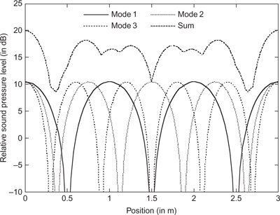
Figure 6.40 The composite effect of adjacent modes on the spatial variation in a room.

Figure 6.41 The way to guarantee that at least three modes are excited by a given frequency.
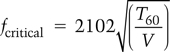
This equation shows that the critical frequency is inversely proportional to the square root of the room volume and is proportional to the square root of the reverberation time, which is also proportional to the cube root of the volume, if the absorption remains constant, as discussed earlier. The net result of this is that, as expected, the critical frequencies for larger rooms are generally lower than those of smaller ones. Thus big rooms are acoustically “large” as well.
As an example let us calculate the critical frequency of our typical living room.
Example 6.12
What is the critical frequency of a room whose surface area is 75 m2, and whose volume is 42 m3? What is the critical frequency of the same room if the average absorption coefficient is 0.2?
Using the first equation calculate the lowest bound on the critical frequency using the mean free path as:

Using the second equation calculate the critical frequency using the reverberation time. Firstly, calculate the reverberation time as:
![]()
Then, using the second equation, calculate the critical frequency as:
![]()
The second equation predicts a slightly lower critical frequency compared with the first one. However, the agreement is surprisingly good. Although the modal overlap has been calculated using a reverberation time, and hence a diffuse field assumption, this is probably just valid at this frequency, which represents the boundary between the two regions. The critical frequency results show that, for this room, frequencies below 213 Hz must be analyzed using modal decay time rather than reverberation time.
6.3 Absorption Materials
Absorption materials are clearly important in their effects on the acoustics, and this section briefly looks at the factors which affect the performance of these materials and their effects on an acoustic space.
There are two basic forms of absorption materials—porous absorbers and resonant absorbers—which behave differently because their mechanisms of absorption are different.
6.3.1 Porous Absorbers
Porous absorbers, such as carpets, curtains and other soft materials, work due to frictional losses caused by the interaction of the velocity component of the sound wave with the surface of the absorbing material. In Chapter 1 we saw that the velocity component arose because the air molecules had to move between the compression and rarefaction states. A given pressure variation will require a greater pressure gradient, and hence higher peak velocities, as the wavelength gets smaller with rising frequency. Because the pressure gradient of a sound wave increases with frequency, the friction due to interaction with a surface will also increase with frequency and therefore the absorption of these types of material also rises with frequency. Clearly the larger the surface area available for interaction, the higher the friction and therefore the absorption. This means that porous materials, which consist of a large number of fibers per unit volume, such as high-density rock-wool or fiberglass, and plush carpets, will tend to have a high-level absorption. This also explains why curtains which are draped to a fraction of their cloth area absorb more strongly than ones which are flat.
Typical absorption curves for porous absorbers are shown in Figure 6.42. Because porous absorbers interact with the velocity component of the sound wave, they are affected by the space between them and the wall and their thickness. This is due to the fact that at the exposed surface of a hard surface, such as a wall, the velocity component is zero whereas at a quarter of a wavelength away from the wall the velocity component will be at a maximum, as shown in Chapter 1, and so a porous material will absorb more strongly at frequencies whose quarter wavelength is less than either the spacing of the material from the wall, or the thickness of the material if it is bonded directly to the surface.
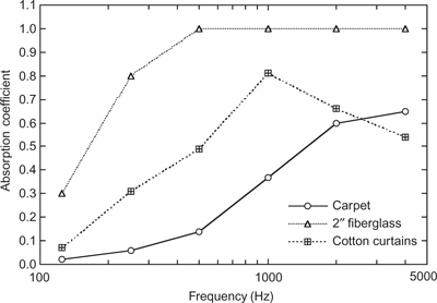
Figure 6.42 Typical absorption curves for panel absorbers.
This effect is shown in Figure 6.43. Although in principle there could be a variation in the absorption coefficient as the frequency increases above the quarter wavelength point, due to the inherent variation of the velocity component as a function of wavelength at a fixed distance from a surface, in practice this does not occur unless the material is quite thin.
Figure 6.43 The effect of spacing a porous absorber away from a hard surface.
Resonant absorbers, such as wood paneling, work because the incident sound energy causes vibrations in the absorber and these are converted to frictional losses within the absorbing structure itself. This makes them sensitive to the pressure component of the sound wave and so they work well when attached to walls. The typical construction of a panel absorber is shown in Figure 6.44. In the case of wood panels the absorption is due to the internal frictional losses in the wood. In the perforated absorber, discussed later, it is due to the enhancement of velocity that happens in the perforations at resonance. Because the absorbers are resonant their absorption increases at low frequencies, as shown in Figure 6.45.

Figure 6.44 Typical construction of a panel absorber.

Figure 6.45 Typical absorption curves for panel absorbers.
The resonant characteristics of these absorbers enable them to be tuned to low frequencies and so allow them to have absorption characteristics which complement those of porous absorbers. The peak absorption frequency of a resonant absorber is a function of the space behind the absorber and the effective mass of the front panel. To use an analogy with a spring and weight, the rear cavity acts like a spring whose stiffness is inversely proportional to the depth of the cavity and the effective mass per unit area of the front panel determines the size of the weight. As the spring gets less stiff and the effective mass becomes greater, the resonant frequency drops. Thus deeper rear cavities result in lower resonances for both types. For the panel absorbers the mass per unit area of the panel is directly related to the effective mass, so heavier front panels result in a lower resonant frequency. The resonance frequency of panel absorbers can be calculated using the following equation:
![]()
where M = | panel’s mass per unit area (in kg m–2) |
and d = | depth of the airspace (in m) |
However, this equation must be applied with some caution because it assumes that the panel has no stiffness. This assumption is valid for thin panels but becomes less applicable as the panel becomes thicker and thus more stiff.
Another form of resonant absorber is based on the use of the resonance that occurs when air is trapped in a tube above an air space. This type of resonance is called a Helmholtz resonance and is the resonance that occurs in a beer bottle when you blow across it. The cavity acts like a spring and the air in the tube above the cavity acts like the mass. The construction of this type of absorber consists of a perforated panel above an airspace, as shown in Figure 6.46.

Figure 6.46 Typical absorption curves for Helmholtz resonant absorbers
For the perforated panels the effective mass is a function of both the depth of the perforations and their effective area as a percentage of the total area. Their effective mass increases as the depth increases and the percentage hole area reduces. Typical absorption curves for this type of absorber are shown in Figure 6.47. This type of absorber is often used to add extra absorption at high-bass and low-midrange frequencies.

Figure 6.47 Typical absorption curves for wideband absorbers.
6.3.4 Wideband Absorbers
It is possible to combine the effects of porous and resonant absorbers to form wideband absorbers. A typical construction is shown in Figure 6.48 and its performance is shown in Figure 6.49. As with all absorbers using rock-wool or fiberglass one must take precautions to prevent the egress of irritating fibers from the absorber into the space being treated.

Figure 6.48 Construction of a wideband absorber.

Figure 6.49 Typical absorption curves for wideband absorbers.
An alternative means of achieving wideband absorption is to use a large depth of porous absorber, for example one meter, and this can provide effective absorption with a flat frequency response, but at the cost of considerable depth.
6.3.5 Summary
With these basic types of absorption structures it is possible to achieve a high degree of control over the absorption coefficient in a room as a function of frequency. In many cases much of the required absorption can be achieved by using materials which fit naturally in the room. For example, much baroque music was performed in the halls of mansions which had a balanced acoustic due to the extensive use of wood paneling in their decoration. This paneling acted as an effective low-frequency absorber and, in conjunction with the flags, drapes and tapestries that also decorated these spaces, provided the necessary acoustic absorption.
As well as absorption it is essential that the sound be diffused when it strikes a surface. Ideally we want the acoustic equivalent of a matt surface. Unfortunately most surfaces, including large areas of absorbing material, act like acoustic mirrors, with varying shades of darkness. In order to have a matt surface one needs a “bumpy wall” and many things can be used to provide this. Unfortunately the bumps need to be at least an eighth, and preferably a quarter, of a wavelength in size to be effective. This results in the requirement for very large objects at low frequencies (1.25–2.5 m at 34 Hz) and very small objects at higher frequencies (1.25–2.5 cm at 3.4 kHz). If the objects are too small, that is, less than one eighth of a wavelength, they will not diffuse properly; if they are too big, that is, greater than about a half a wavelength, they will behave as acoustic mirrors in their own right and so will not diffuse effectively.
Clearly effective diffusion is a difficult thing to achieve in an ad hoc manner. Curved and angled structures can help at mid and high frequencies, and at very high frequencies, greater than about 4 kHz, the natural rough textures of materials such as brick and rough cut stone are effective. Because of the need to achieve well-defined diffusion characteristics, diffusion structures based on patterns of wells whose depths are formally defined by an appropriate mathematical sequence have been proposed and used (Schroeder, 1975 and D’Antonio and Konnert, 1984). The design of these structures is quite involved and the reader is directed to the references if they want more information. However, a brief description of how they work is as follows.
6.4.1 How Diffusers Work
Consider a hard surface consisting of bumps of height d. Also consider an acoustic wavefront approaching it from a normal direction. The way this wavefront is reflected will depend on the height of the bumps relative to its wavelength. Let us consider three cases:
- In the case of d << λ the surface will behave like a flat surface and specularly reflect the wavefront.
- In the case of d =
 the wavefronts which are reflected from the front of the bumps are reflected
  earlier than those from the surface. This means that in the normal direction the wavefronts cancel and so no sound pressure is propagated in this direction. However, there has been no energy loss in the system so the wavefront must be reflected in some direction. In fact as one moves away from the normal direction the relative path lengths between the bump and the surface become less and the amplitude of the wavefront increases. This is the basic principle behind diffusion using hard reflectors. That is, the diffusing surface modifies the phase of the wavefronts so that the reflected wave must propagate in directions other than the specular direction.
 - In the case of d = the wavefronts from the bumps and surface are delayed by λ and so arrive back in phase. Thus the bumps disappear and the surface behaves as if it were flat. That is, it behaves like a specular reflector.
So, one has a problem: a regular sequence of bumps will diffuse but only at frequencies at which it is an odd multiple of ![]() . Note also that these frequencies will depend on the angle of incidence of the incoming wavefront.
. Note also that these frequencies will depend on the angle of incidence of the incoming wavefront.
What is required is a pattern of bumps which alter the phases of the incident waves in such a way that two objectives are satisfied:
The sound is scattered in some “optimum” manner.
The scattering is optimum over a range of frequencies.
These objectives can be satisfied by several different sequences, but they share two common properties:
- The Fourier transform of the sequence is constant except for the d.c. component which may be the same or lower. This satisfies objective (1) because it can be shown that reflection surfaces with such a property scatter energy equally in all directions. The effect of a reduced d.c. component is to further reduce the amount of energy which is reflected in the specular direction.
- The second desirable property of these sequences is that the Fourier transform is unaffected if the wavelength of the incident sound varies. This has the effect of changing the scale of the sequence, but again one can show that the resulting sequence still has the same properties as the original sequence.
Both the above properties arise because the sequences work by perturbing the wavefronts over a full cycle of the waveform. Such sequences are called phase reflection gratings because they perturb the phase of the wavefront.
To make this a little clearer, let us consider two sequences which are used for diffusers.
Quadratic residue sequences well depth = n2 mod p where p is a prime number. If p = 5 this gives a set of well depths of
0, 1, 4, 4, 1, 0, 1, …, etc.
so the sequence repeats with a period of 5.
Primitive root sequences well depth = an mod p where p is a prime and a is a suitable constant called a primitive root. For a = 2 and p = 5 we get the sequence
1 2, 4, 3, 1, 2, …, etc.
Here we have a sequence which has a period of 4 (5 − 1).
At the lowest design frequency for these examples a well of depth 5 would correspond to ![]() . At higher frequencies the sequences still have the same properties and thus scatter sound effectively. However, when the frequency gets high enough so that
. At higher frequencies the sequences still have the same properties and thus scatter sound effectively. However, when the frequency gets high enough so that ![]() becomes equal to the minimum difference in depths (1) then the surface again becomes equivalent to a flat surface.
becomes equal to the minimum difference in depths (1) then the surface again becomes equivalent to a flat surface.
The typical construction of these structures is shown in Figure 6.50 and their performance is shown in Figure 6.51.

Figure 6.50 Typical construction of a quadratic residue diffuser.

Figure 6.51 Typical performance of a quadratic residue diffuser compared with a flat plate. (Note that for convenience the responses have normalized to 0dB in the specular direction. In practice the flat plate’s output would be greater in this direction.)
6.4.2 Discussion
As we have seen, these sequences achieve their performance by spreading the phase of the reflected wavefront over at least one cycle of the incident wavefront. In order to do this, their maximum depth must be ![]() at the lowest design frequency. This means that to achieve diffusion a reasonable depth is required. For example, to have effective diffusion down to 500 Hz a depth of 34 cm (13.5 inches) is required. To get down to 250 Hz one would need to double this depth. However, as we have seen, a simple bump of
at the lowest design frequency. This means that to achieve diffusion a reasonable depth is required. For example, to have effective diffusion down to 500 Hz a depth of 34 cm (13.5 inches) is required. To get down to 250 Hz one would need to double this depth. However, as we have seen, a simple bump of ![]() can provide diffusion, albeit somewhat frequency dependently. This is half the depth of the above sequences and represents the ultimate limit for a diffusing object.
can provide diffusion, albeit somewhat frequency dependently. This is half the depth of the above sequences and represents the ultimate limit for a diffusing object.
It is possible to have sequences which achieve the phase scatter required for good diffusion using a depth closer to ![]() at the lowest frequency (4) and so allow better performance diffusers in restricted spaces. However, even
at the lowest frequency (4) and so allow better performance diffusers in restricted spaces. However, even ![]() at low frequencies is often too large to be useful. What one really requires is a diffuser which is effective without using any depth!
at low frequencies is often too large to be useful. What one really requires is a diffuser which is effective without using any depth!
6.4.3 Amplitude Reflection Gratings
It is not just physically observable bumps on the wall that can cause diffusion of the sound. In fact any change in the reflecting characteristics of the surface will cause diffusion. The change from an absorbing region on a wall to a reflecting one is an example of a change that will cause the sound to scatter. Thus it is always better to distribute the absorption in small random amounts around a room rather than concentrate it in one particular area. As well as encouraging diffusion this strategy will avoid the possibility that some modes might shuttle between surfaces with minimum absorption. There are also mathematically-based procedures for the optimum placement of absorbing materials to encourage diffusion; for more details on this see Angus (1995). What is required is an amplitude weighting, that is, a pattern of absorbers, which gives a flat Fourier transform.
The most obvious sequences to consider are binary, that is, they contain only levels 0 and 1 where 1 represents reflection from a hard surface and 0 represents absorption from some form of absorbing material. Clearly not all acoustic absorbers are 100% absorbing but this can be simply allowed for by using (1-absorption) instead of zero in the sequence. The net effect of less than 100% absorption would be to increase the level of the specular component. Of the many possible binary sequences, m-sequences would seem to be a good starting point as they have desirable Fourier properties. There are many other bi-level sequences which have flat Fourier transforms but m-sequences are well documented.
Thus amplitude reflection gratings consist of a surface treatment which consists of strips of absorbing material, whose width is less than ![]() at the highest frequency of use, laid out in a pattern in which strips of absorber represent zero and strips of reflecting wall represent 1 (see Figure 6.52). Note that because we are not depending on depth we do not have a low-frequency limit to the range of diffusion, only a high-frequency limit which is a function of the width of the strips.
at the highest frequency of use, laid out in a pattern in which strips of absorber represent zero and strips of reflecting wall represent 1 (see Figure 6.52). Note that because we are not depending on depth we do not have a low-frequency limit to the range of diffusion, only a high-frequency limit which is a function of the width of the strips.

Figure 6.52 Simple implementation of a length 15 one-dimensional Binary Amplitude Diffuser.
m-sequences are pseudo-random binary sequences that can be easily generated by software or hardware.
A two-dimensional example of an amplitude reflection grating is shown in Figure 6.53. Amplitude gratings provide some diffusion although they cannot be as good at diffusing as phase reflection gratings. But, because of their size, they are useful at low frequencies. It also is possible to develop curved diffusion structures, although there are no simple mathematical recipes for them. For further details see Cox (1996). Other structures are possible and the reader is referred to the references for more information.

Figure 6.53 An implementation of a length 1023 two-dimensional Binary Amplitude Diffuser (white dots are holes over absorber).
6.5 Sound Isolation
No discussion of the quality of sound in a room would be complete without a brief discussion of how to keep unwanted sound from entering a room, or how to keep the wanted sound in, so as not to disturb the pleasure of people inside or outside it.
The first thing to note is that just because a material is a good absorber of sound doesn’t mean that it is a good isolator of sound. In fact most absorbing materials are terrible at sound isolation. This is because, in the sound isolation case, we are interested in the amount of sound that travels through a structure rather than the amount that is absorbed by it, as shown in Figure 6.54. A poor value of sound isolation would be around 20 dB yet it corresponds to only one hundredth of the sound being transmitted. A good absorber with an absorption coefficient of 0.9 would let one tenth of the sound through, which corresponds to a sound isolation of only 10 dB! As we are more interested in sound isolations of 40 dB as a minimum, absorption is clearly not the answer.

Figure 6.54 Sound transmission versus sound absorption in a material
6.5.1 Ways of Achieving Sound Isolation
There are only two ways to achieve sound isolation: using either stiffness or mass. Figure 6.55 shows the attenuation of a partition as a function of frequency and from it one can see that stiffness is effective at low frequencies due to the fact that the sound wave must push against the stiffness of the partition. This is known as the “stiffness-controlled isolation region.” As the frequency rises, the partition needs to move less distance to re-radiate a given level of sound and so it gets less effective until at the resonant frequency of the partition its level of attenuation is at its lowest value. This is due to the fact that at resonance the partition can be moved easily by the incident sound wave and so re-radiates the sound effectively.
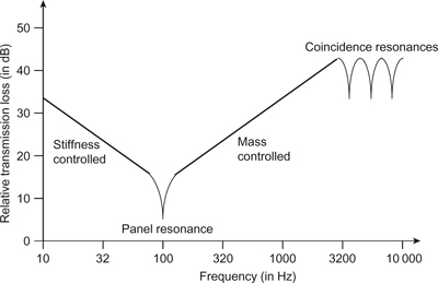
Figure 6.55 Sound transmission as a function of frequency for a partition
As the frequency rises above the partition’s resonant frequency, the mass-controlled region of isolation is entered. In this region, it is the fact that the sound must accelerate a heavy mass that provides the isolation. Because more force is required to move the partition at higher frequencies, the attenuation rises as the frequency rises. At even higher frequencies there are resonances in which both the thickness of the partition and the way sound propagates within it interact with the incident sound to form coincident resonances that reduce the attenuation of the partition. Damping can be used to reduce the effect of these resonances.
Most practical partitions operate in the mass-controlled region of the isolation curve with coincident resonances limiting the performance at higher frequencies. Figure 6.56 shows the attenuation of a variety of single partitions as a function of frequency. In particular note that the plaster board wall has a significant coincidence resonance. The performance of a single partition increases by 3 dB every time its mass is doubled but the coincidence resonances move lower in frequency as well. These coincidence resonances limit the ultimate performance of single partitions. In addition the cost, and size, of single partitions get unreasonable for large attenuations.

Figure 6.56 Sound transmission versus frequency for typical partitions
6.5.2 Independent Partitions
The solution is to have two or more partitions which are independent of each other. If the two partitions are truly independent then the total attenuation, or effective sound isolation, is the product of the attenuations of individual partitions, that is, the dB attenuation is the sum of the dB attenuations of the individual partitions. In practice the partitions are not independent although the isolation is improved dramatically, but not as much as would be predicted by simply summing the dB attenuations. Coincidence resonances also reduce the effectiveness of a partition and it is important to ensure that the two partitions have different resonances. This is most easily assured by having them made with either a different thickness, or a different material.
As an amusing example Figure 6.57 shows the measured results, from Inman (1994), for single and double-glazing made with similar and different thicknesses of glass and spacing. Because of the effect of the coincidence resonances the double-glazed unit with 4 mm glass is actually worse than a single pane of 4 mm glass! As the other two curves show, if the glass is dissimilar the result is much improved, and is further improved if the spacing is increased so as to reduce the coupling between the individual partitions. Often, absorbing material is placed in the cavity between the two partitions to reduce the effect of coincidence resonances but it is important to ensure that the absorbing materials do not make contact with the two partitions or else flanking may occur.

Figure 6.57 Sound transmission versus frequency for single and double-glazing.
6.5.3 Flanking Paths
Flanking paths, which are the main limitation to sound isolating structures, arise when there are other paths that the sound can travel through in order to get round, that is, flank, the sound isolating structure, as shown in Figure 6.58. Typical paths for flanking are the building structure, heating pipes, and, most commonly, ventilation systems or air leaks. The effect of the building structure can be reduced by building a “floating room,” as shown in Figure 6.59, which removes the effect of the building structure by floating the room on springs away from it.

Figure 6.58 Flanking paths in a structure.

Figure 6.59 Floating room construction.
In practice, ensuring that no part of the building is touching the floating room by any means (plumbing pipes and electrical wiring conduits are popular offenders in this respect) is extremely difficult. The effect of ventilation systems and air leaks is also a major source of flanking in many cases. In fact in the domestic situation the sound isolation is almost entirely dominated by air leaks and draught paths, and it is the removal of these that allow double-glazing salesmen to advertise a dramatic improvement in sound isolation, despite having two 4 mm panes of glass in the double-glazing.
So in order to have good sound isolation one needs good partitions and an airtight, draught-free, structure. Achieving this in practice while still allowing the occupants to breathe is a challenge.
6.6 The Effect of Room Boundaries on Loudspeaker Output
If we wish to listen to sound from loudspeakers we must also consider the effect the room has on them. We have already seen that the reverberant field colors the sound of the loudspeakers depending on its level relative to the direct sound. However, the walls of the room also have an effect.
The effect of the presence of boundaries, such as walls, on the low-frequency output of loudspeakers is well known (Allison, 1980). Many methods of ameliorating these effects have been proposed, ranging from careful positioning to special speaker designs that try to remove the effect of the boundaries.
When a speaker is placed near a reflecting boundary an image source is formed due to that reflecting boundary, as shown in Figure 1.28 in Chapter 1. Thus when a speaker is placed near three reflecting boundaries three image sources are formed, as shown in Figure 6.60. The effect of these image sources, which represent reflections from the boundary, is to modify the local acoustic impedance seen by the loudspeaker. Because a dynamic speaker is mass controlled in its normal working region it forms a high impedance source and therefore the radiated power is affected by the local impedance variations.

Figure 6.60 Images formed at the nearest three reflecting boundaries to a loudspeaker.
Waterhouse (1955) extended work by Rayleigh (1964) and confirmed experimentally that the power output of a source is affected the presence of boundaries, for example the walls in a room. The effect of this is plotted in Figures 6.61 and 6.62 for two different boundary conditions. In one case, all the dimensions are the same (Figure 6.61); in the other, they are different to minimize the effects (Figure 6.62). It does not matter from which surface a speaker has a particular spacing. However, it is important that the dimensions are in the correct ratio. Note that in these graphs the x-axis is the number of wavelengths with respect to the distance “x” from the boundary. This is analogous to frequency, but scaled as with respect to distance. Thus if “x” equaled one meter a value of “1” on the x-axis would correspond to a wavelength of one meter (344 Hz); if “x” equaled half a meter a value of “1” on the x-axis would correspond to a wavelength of half a meter (688 Hz), and so on.

Figure 6.61 Loudspeaker boundary interaction “non-optimum” placement
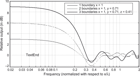
Figure 6.62 Loudspeaker boundary interaction “optimum” placement
From these graphs, we can see two main things:
If the dimensions are the same then one has a low-frequency response that rises 9 dB above the mid-band response, and that has significant variation over the frequency range – in particular when the distance between the loudspeaker and the boundaries is just above a quarter of a wavelength
By placing the speaker carefully, with respect to the boundaries, one can eliminate some of the variation in the response. However, one still has a 9 dB rise in response at low frequencies. This is well known and the 9 dB rise at low frequencies is inherent in operating in an environment with three boundaries. In general, the low-frequency responses of loudspeakers designed to be placed close to boundaries is tailored to compensate for it.
In the case of flush mounting the speaker in the wall, the result is slightly different. Now the effect of the mounting surface extends to very high frequencies and therefore the number of surfaces that affect the low-frequency response reduces to two. This means the maximum low-frequency rise becomes 6 dB and the optimum ratios of placement change.
In the modal region the whole room affects the loudspeaker’s output. In this region the output of the speaker is strongly affected by how the modal shapes in the room interact with the loudspeaker. As discussed with regard to bowed instruments in Chapter 4, the point of excitation strongly affects which modes are excited. This effect also happens with loudspeakers, except, unlike the bowed string, it is now a three-dimensional problem! It is sometimes possible to find compromise positions for the loudspeakers that excite the room modes as evenly as possible but, needless to say, this is very room-, and speaker-, dependent.
6.7 Reduction of Enclosure Diffraction Effects
The other aspect of loudspeakers is the effect of diffraction around the enclosure shape. If the speaker is wall mounted this is not important, but for free-standing speakers it is an issue.
In 1950, Olson (1969) demonstrated, experimentally, that the enclosure shape and size significantly affect the frequency response of a loudspeaker, due to diffraction effects. These diffraction effects can occur at any frequency where the wavelength is of similar size, or smaller than the box. This means that they can occur in any small enclosure, such as a top mounted tweeter. They can also occur in the main cabinets if there are drivers whose frequency ranges produce wavelengths of appropriate dimensions relative to the box sizes.
In the context of loudspeaker design it is the bounded to unbounded case that is important as this is what happens when a sound wave from a loudspeaker reaches the edge of the front face of an enclosure. In this situation, the wave is making a transition from being bounded by the front of the enclosure to being unbounded, as shown in Figure 6.63. The consequential reflections cause disturbances to the frequency response of the loudspeaker because they interfere with the main output.

Figure 6.63 Reflection due to bounded-unbounded transition at a loudspeaker cabinet edge.
Some of Olson’s results are shown in Figure 6.64. His research showed that the shape of an enclosure should be, ideally, curved and small with respect to the wavelengths in use. He also found that the shape with the smoothest response was spherical; see Figure 6.64(b). However, he also showed that non-spherical shapes, such as the truncated pyramid and rectangular parallelepiped combination shown in Figure 6.64(c), could also give good performance.

Figure 6.64 Diffraction effects due to different enclosure (from Olson, 1969)
Although an ideal shape is spherical, as shown in Figure 6.65(a), other curved shapes offer some practical advantages. In particular, a truncated ellipsoidal shape, as shown in Figure 6.65(b), offers a good diffraction performance and some flexibility in the volume for a given frontal area. This is important for several reasons.
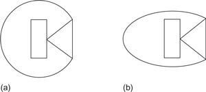
Figure 6.65 A comparison of spherical and ellipsoidal loudspeaker enclosures
Firstly, in order to maintain an approximately spherical shape, a spherical enclosure must have a diameter that is significantly larger than the diameter of the drive unit. In Figure 6.65a the sphere’s diameter is twice that of the drive unit. If the diameter of the sphere equaled that of the drive unit the enclosure shape would be a half sphere, which would have a poorer performance than a sphere.
Secondly, the volume of the enclosure interacts with the drive unit to set a lower frequency limit for the loudspeaker. Clearly, a sphere cannot have a diameter that is less than the diameter of the drive unit. Truncated ellipsoidal shapes, as shown in Figure 6.65(b), have an additional degree of freedom that, within reason, allows one to set the volume independently of the diameter of the drive unit.
Finally, a sphere suffers from coincident resonances that can affect the frequency and time response of the loudspeaker. A truncated ellipsoidal shape, as shown in Figure 6.65(b), has non-coincident resonances that can result in a smoother response.
Olson’s results indicate that truncated ellipsoidal shapes, as shown in Figure 6.65, can achieve nearly as good results as a sphere.
Diffraction at bass frequencies is generally less of a problem, because the wavelengths are large compared with the cabinet size. However, if the main cabinet contains midrange units then it must also take account of diffraction effects. As this enclosure must also contain the bass units, and must sit on a surface, it is not possible to have a spherical enclosure. Instead, the curvature can only be arranged in the vertical axis.
Olson (1969) also examined this condition and some of his results are shown in Figure 6.66. From Figure 6.66(a) we can see that the rectangular parallelepiped enclosure has significant diffraction effects. This is despite the fact that the driver is mounted off-center, a strategy that reduces the effect of diffraction by reducing the number of coincidence effects. The cylindrical enclosure, Figure 6.66(b), does not seem to offer much improvement. This is due to both the presence of two edges, and to the coincidence effects caused by the central location of the driver between those two edges. An off-center driver would have improved the results.

Figure 6.66 Diffraction effects due to enclosures with at least two flat sides (from Olson, 1969).
The rectangular truncated pyramid and rectangular parallelepiped combination enclosure with an off-center driver, Figure 6.66(c), offers a considerable improvement. If the front surfaces are smooth curves instead of facets, the response will be even better, and will have only been limited by the abrupt transitions from the rear of the cabinet. The main consequence of these results is that wherever possible the enclosure should be curved near the drive-units and that the drive-units should not be mounted in the center of the enclosure. In practice, they will have to be mounted centrally in the horizontal direction, but they do not need to be so in the vertical direction. Under these circumstances, the most appropriate shape is circular. However, for the reasons outlined previously, an ellipsoidal shape is often more appropriate.
In this chapter we have examined how the space in which the sound is reproduced affects both its reproduction and perception. We have seen how the room affects the output of loudspeakers, and other sound sources. We have also analyzed various situations and examined various techniques for achieving a good acoustic environment for hearing music.
References
Allison, R.F., 1980. The influence of room boundaries on loudspeaker power output. In: Cooke, R.E. (Ed.), Loudspeakers – An Anthology, vol. 1. The Audio Engineering Society, New York, pp. 353–359.
Angus, J. A. S. (1995). Sound diffusers using reactive absorption gratings. Audio Eng. Soc. Conv. 98, 25–28 Feb, Paris, preprint #3953.
Cox, T.J., 1996. Designing curved diffusers for performance spaces. J. Audio Eng. Soc. 44 (5), 354.
Cox, T.J., D’Antonio, P., Avis, M.R., June 2004. Room sizing and optimization at low frequencies. J. Audio Eng. Soc. 52 (6), 640–651.
D’Antonio, P., Konnert, J.H., April 1984. The reflection phase grating diffusor: design theory and application. J. Audio Eng. Soc. 32 (4), 228–238.
Inman, C., Sept.–Oct. 1994. A practical guide to the selection of glazing for acoustic performance in buildings. Acoust. Bull. 19 (5), 19–24.
Olson, H.F. (1969). Direct radiator loudspeaker enclosures. Journal of the Audio Engineering Society, January. Vol. 17, Number 1, 22–29. Note, originally presented at the Second Annual Convertion of the Engineering Society, 27 October, 1950.
Rayleigh, Lord., 1964. Work Done by Detached Sources. In: Scientific Papers, vols. 5–6. Dover, New York, pp. 135–141.
Schroeder, M.R., Jan. 1975. Diffuse sound reflection by maximum length sequences. J. Acoust. Soc. Am. 57 (1), 149–150.
Walker, R., 1996. Optimum dimension ratios for small rooms. Audio Eng. Soc. Conv. 100, preprint #4191.
Waterhouse, R.V, Mar. 1955. Output of a sound source in a reverberation chamber and other reflecting environments. J. Acoust. Soc. Am. 27 (2).
Further Reading
Angus, J.A.S., McManmon, C.I., Dec. 1998. Orthogonal sequence modulated phase reflection gratings for wide-band diffusion. J. Audio Eng. Soc. 46 (12).
D’Antonio, P., Cox, T., Nov. 1998. Two decades of diffuser design and development, Part 1: applications and design. J. Audio Eng. Soc. 46 (11).
Newell, P., 2003. Recording Studio Design. Focal Press, Oxford.