POST-PRODUCTION/IMAGE MANIPULATION

RESOLUTION AND IMAGE FORMAT CONSIDERATIONS

Scott Squires

Formats

Capture Format

The capture format for a film is decided in pre-production by the Director and Director of Photography (DP) along with the Production Designer and the VFX Supervisor. Creative choices along with camera size, post workflow, and costs are all a factor when determining the particular format.

Typically the choices are a 35mm film camera or digital camera (HD resolution or higher). With 35mm film there is the choice of a 1:85 ratio¹ (traditional aspect ratio) or 2:35/2:40 ratio (anamorphic or widescreen). The ratios are achieved either by using an anamorphic lens that squeezes the image or by using a Super 35 format² to record as a flat image that will be extracted. If the final film is to be shown in IMAX format,³ then this will need to be considered as well since IMAX requires higher resolution for the best results.

There are a number of variations when it comes to digital capture formats. The selection of the codec⁴ used will have a large impact on the quality of the image as well as the storage requirements for the initial capture.

Film needs to be scanned before doing digital visual effects, but currently film supplies a higher resolution and greater dynamic range than digital formats. Digital formats don’t require scanning and therefore might provide a cost and time savings when importing the footage for visual effects work.

Film stock choices will be important for the style of the film and the visual effects work. Green and blue screens require film stock consideration to ensure the color response and resolution is sufficient to pull keys. This is especially true in digital formats where some codecs produce full color and others produce reduced color response and compression artifacts (which is a potential problem for blue or green screens). Full-color digital is usually referred to as 4:4:4, but some codecs provide image data that is sampled at lower color resolution (such as 4:2:2), which results in matte edges that are very blocky and obvious. See Digital Cinematography and Greenscreen and Bluescreen Photography in Chapter 3 for more information.

Whatever capture source is chosen will set the specifics for graining and degraining in post and subtle but important issues such as the shape and look of lens flares, out-of-focus highlights, and image edge characteristics so the finished visual effects shots match the live-action shots.

File Formats

Each company determines what image formats they will use internally. A scanning company may supply DPX⁵ images but the visual effects company may import these and work internally with EXR⁶ or other formats. Footage from digital cameras is imported and then resaved in the internal format of choice. Intermediate file formats are chosen to maintain the highest level of quality throughout the pipeline. This avoids any artifacts or other problems when combining images, processing them, and resaving them through a few generations.

File format issues also come into play when determining what to supply editorial. These could be specific QuickTimes or other formats depending on the editorial workflow setup. This should be sorted out in pre-production so the visual effects pipeline includes being able to export in the correct format, including color and gamma space.

Film delivery formats for exporting the final shots are another file format that needs to be chosen. In the past, film-outs⁷ from digital files to film were required for film-based projects. Now most film projects use a digital intermediate (DI) process. All live-action shots are scanned and imported for DI to be color corrected. In this case the finished visual effects digital files are submitted to the DI company in their requested format.

Target Format

Most films are delivered for both film and digital projection distribution. This is typically handled by the DI company and film labs. In some cases a film will be released in IMAX as well. This will require a special film-out process.

Transport

All of these digital files need to be moved from one location to another—both within a visual effects company and between the visual effects company and other vendors on the project. Files are typically distributed locally within the company using Ethernet. When going to or from another company, the images may be transferred by secure high-speed data connections or they may be transferred to large hard drives and physically shipped. In some cases storage tapes can be shipped if they are compatible. HD input and final output can be done using HD tape transfers although hard drives and Internet connections are probably more common.

Resolution

Most film production has been done at 2k (2048 pixels wide). As more 4k (4096 pixels wide) digital projectors become available, there has been a push to use 4k throughout the entire process. While this does technically increase the quality of the image, some issues still need to be addressed. To support a given resolution, every step in the process has to maintain that same resolution or higher. If the initial source is HD resolution, then working in 4k would require an initial resize and the up-ressed (resized larger) results would not provide as much of an increase in quality as a 4k film scan source would. As with digital still cameras, diminishing returns are seen as the pixel count goes up.

Scanning is frequently done at a higher resolution to allow better quality images even if they will be scaled down. Resolution of 4k will allow the full detail typical of a typical 35mm film shot to be captured and maintained through the production pipeline. This allows the digital images to be the best they can be from 35mm film; in addition, the images will be less likely to require rescanning for future formats.

However, a number of issues should be reviewed before settling on the resolution. A resolution of 4k means that the image will be twice as many pixels wide and twice as many vertically. This is four times the amount of data required of a 2k image. Although not every process is directly linked to the size, most visual effects steps are. When visual effects companies went from 8-bit per channel to 16-bit floating point, the size of the image data doubled. This increase in pixel resolution will require four times as much data.

A 4k image will take four times as much storage space on disk so a given hard drive will now hold only a one-quarter of the frames it could hold for 2k projects. It will also take longer to load and save images. This increases the time the visual effects artists may have to wait on their workstations. Some software may be less responsive since the image is occupying much more memory, and live playback will be an issue since only one-quarter of the frames can be loaded. Also, 4k requires more pixels to paint if one needs to work in full detail. Transferring images to other machines on the network or off site will also take four times as long. Archiving of material will require more time and storage as well.

A typical monitor does not support the full 4k, so users will need to resize images to 2k or less to see the entire image and then zoom in to see the full resolution. Projection equipment at the visual effects company will need to support 4k if pixels are to be checked on the big screen. Any hardware or software that doesn’t support 4k efficiently will have to be upgraded or replaced. In some steps, 2k proxies can be used just as video resolution proxies are sometimes used in normal production. This can be done for testing, initial setups, and processes where the image is a guide such as rotoscoping.

How noticeable will the results be? If the results are split screened or toggled on a correctly configured large-screen projection, then they may be obvious. But when projected without a direct comparison, it’s not likely the audience at the local theater will notice. For a number of years after digital visual effects came into being, visual effects were done on very large films at slightly less than 2k with 8-bit log color depth. These shots were intercut directly with film. Not too many people complained to the theater owners. Some theatrically released films were shot in the DV format (Standard Definition Digital Video; typically for consumer video cameras). These were used for specific purposes but in most cases audiences will ignore the technical issues and focus on the story once the film is under way. (Assuming it’s a good story being well told.)

Today Blu-ray DVD movies are available. They are a higher resolution and use a better codec than regular DVDs, but many people are finding the upres (resizing) of their old DVDs to be pretty good. When DVDs came out there was a very large quality difference and ease of use compared to VHS tapes. People purchased DVD players but the leap from DVD to Blu-ray is not as apparent to the average person so there has been slow acceptance of this new format. Note that high-quality resizing software and hardware also allows 2k film to be resized to 4k probably with better results than expected. This can be done at the very end of the pipeline.

The quality comparisons assume a locked-off camera using the highest resolution of the film. If a film is shot with a very shaky handheld camera with frenetic action and an overblown exposure look, the results may not show a noticeable difference.

Summary

A resolution of 4k will likely be used for visual effects-heavy films and eventually for standard films. At the time of this writing (early 2010), it may or may not make sense for a specific project.

Visual effects companies will need to review their pipelines and ideally run a few simulated shots through to make sure everything handles 4k and to actually check the time and data sizes being used. From this they can better budget 4k film projects since these will cost more and take some additional time.

For the filmmakers and studios that wish to have 4k resolution, they will need to determine whether it is worth the extra cost. With tighter budgets and tighter schedules, it may not make the most sense. Would the extra budget be put to better use on more shots or other aspects of the production? It is unlikely that 4k itself will sell more tickets to a movie, so ultimately it’s a creative call versus the budget.

As new resolutions and formats (such as stereoscopic) are introduced, these will have to be evaluated by the producers and the visual effects companies to see what the impact will be and to weigh the results.

IMAGE COMPRESSION/FILE FORMATS FOR POST-PRODUCTION

Florian Kainz, Piotr Stanczyk

This section focuses on how digital images are stored. It discusses the basics of still image compression and gives an overview of some of the most commonly used image file formats. An extended version of this section, which covers some of the technical details, can be found at the Handbook’s website (www.VESHandbookofVFX.com).

Visual effects production deals primarily with moving images, but unlike the moving images in a television studio, the majority of images in a movie visual effects production pipeline are stored as sequences of individual still frames, not as video data streams.

Since their beginning, video and television have been real-time technologies. Video images are recorded, processed, and displayed at rates of 25 or 30 frames per second (fps). Video equipment, from cameras to mixers to tape recorders, is built to keep up with this frame rate. The design of the equipment revolves around processing streams of analog or digital data with precise timing.

Digital visual effects production usually deals with images that have higher resolution than video signals. Film negatives are scanned, stored digitally, processed, and combined with computer-generated elements. The results are then recorded back onto film. Scanning and recording equipment is generally not fast enough to work in real time at 24 fps. Compositing and 3D computer graphics rendering take place on general-purpose computers and can take anywhere from a few minutes to several hours per frame. In such a non-real-time environment, storing moving images as sequences of still frames, with one file per frame, tends to be more useful than packing all frames into one very large file. One file per frame allows quick access to individual frames for viewing and editing, and it allows frames to be generated out of order, for example, when 3D rendering and compositing are distributed across a large computer network.

Computers have recently become fast enough to allow some parts of the visual effects production pipeline to work in real time. It is now possible to preview high-resolution moving images directly on a computer monitor, without first recording the scenes on film. Even with the one-file-per-frame model, some file formats can be read fast enough for real-time playback. Digital motion picture cameras are gradually replacing film cameras. Some digital cameras have adopted the one-file-per-frame model and can output, for example, DPX image files.

Though widely used in distribution, digital rights management (DRM) technologies are not typically deployed in the context of digital visual effects production. The very nature of the production process requires the freedom to access and modify individual pixels, often via one-off, throwaway programs written for a specific scene. To be effective, DRM techniques would have to prevent this kind of direct pixel access.

Image Encoding

For the purposes of this chapter, a digital image is defined as an array of pixels where each pixel contains a set of values. In the case of color images, a pixel has three values that convey the amount of red, green, and blue that, when mixed together, form the final color.

A computer stores the values in a pixel as binary numbers. A binary integer or whole number with n bits can represent any value between 0 and 2ⁿ – 1. For example, an 8-bit integer can represent values between 0 and 255, and a 16-bit integer can represent values between 0 and 65,535. Integer pixel value 0 represents black, or no light; the largest value (255 or 65,535) represents white, or the maximum amount of light a display can produce. Using more bits per value provides more possible light levels between black and white to use. This increases the ability to represent smooth color gradients accurately at the expense of higher memory usage.

It is increasingly common to represent pixels with floating point numbers instead of integers. This means that the set of possible pixel values includes fractions, for example, 0.18, 0.5, etc. Usually the values 0.0 and 1.0 correspond to black and white, respectively, but the range of floating point numbers does not end at 1.0. Pixel values above 1.0 are available to represent objects that are brighter than white, such as fire and specular highlights.

Noncolor Information

Digital images can contain useful information that is not related to color. The most common noncolor attribute is opacity, often referred to as alpha. Other examples include the distance of objects from the camera, motion vectors or labels assigned to objects in the image. Some image file formats support arbitrary sets of image channels. Alpha, motion vectors, and other auxiliary data can be stored in dedicated channels. With file formats that support only color channels, auxiliary data are often stored in the red, green, and blue channels of a separate file.

Still Image Compression

A high-resolution digital image represents a significant amount of data. Saving tens or hundreds of thousands of images in files can require huge amounts of storage space on disks or tapes. Reading and writing image files requires high data transfer rates between computers and disk or tape drives.

Compressing the image files, or making the files smaller without significantly altering the images they contain, reduces both the amount of space required to store the images and the data transfer rates that are needed to read or write the images. The reduction in the cost of storage media as well as the cost of hardware involved in moving images from one location to another makes image compression highly desirable.

A large number of image compression methods have been developed over time. Compression methods are classified as either lossless or lossy. Lossless compression methods reduce the size of image files without changing the images at all. With a lossless method, the compression and subsequent decompression of an image result in a file that is identical to the original, down to the last bit. This has the advantage that a file can be uncompressed and recompressed any number of times without degrading the quality of the image. Conversely, since every bit in the file is preserved, lossless methods tend to have fairly low compression rates. Photographic images can rarely be compressed by more than a factor of 2 or 3. Some images cannot be compressed at all.

Lossy compression methods alter the image stored in a file in order to achieve higher compression rates than lossless methods. Lossy compression exploits the fact that certain details of an image are not visually important. By discarding unimportant details, lossy methods can achieve much higher compression rates, often shrinking image files by a factor of 10 to 20 while maintaining high image quality.

Some lossy compression schemes suffer from generational loss. If a file is repeatedly uncompressed and recompressed, image quality degrades progressively. The resulting image exhibits more and more artifacts such as blurring, colors of neighboring pixels bleeding into each other, light and dark speckles, or a “blocky” appearance. For visual effects, lossy compression has another potential disadvantage: Compression methods are designed to discard only visually unimportant details, but certain image-processing algorithms, for example, matte extraction, may reveal nuances and compression artifacts that would otherwise not be visible.

Certain compression methods are called visually lossless. This term refers to compressing an image with a lossy method, but with enough fidelity so that uncompressing the file produces an image that cannot be distinguished from the original under normal viewing conditions. For example, visually lossless compression of an image that is part of a movie means that the original and the compressed image are indistinguishable when displayed on a theater screen, even though close-up inspection on a computer monitor may reveal subtle differences.

Lossless Compression

How is it possible to compress an image without discarding any data? For example, in an image consisting of 4,000 by 2,000 pixels, where each pixel contains three 16-bit numbers (for the red, green, and blue components), there are 4,000 × 2,000 × 3 × 16 or 384,000,000 bits, or 48,000,000 bytes of data. How is it possible to pack this information into one-half or even one-tenth the number of bits?

Run-Length Encoding

Run-length encoding is one of the simplest ways to compress an image. Before storing an image in a file, it is scanned row by row, and groups of adjacent pixels that have the same value are sought out. When such a group is found, it can be compressed by storing the number of pixels in the group, followed by their common value.

Run-length encoding has the advantage of being very fast. Images that contain large, uniformly colored areas, such as text on a flat background, tend to be compressed to a fraction of their original size. However, run-length encoding does not work well for photographic images or for photoreal computer graphics because those images tend to have few areas where every pixel has exactly the same value. Even in uniform areas film grain, electronic sensor noise, and noise produced by stochastic 3D rendering algorithms break up runs of equal value and lead to poor performance of run-length encoding.

Variable-Length Bit Sequences

Assume one wants to compress an image with 8-bit pixel values, and it is known that on average 4 out of 5 pixels contain the value 0. Instead of storing 8 bits for every pixel, the image can be compressed by making the number of bits stored in the file depend on the value of the pixel. If the pixel contains the value 0, then a single 0 bit is stored in the file; if the pixel contains any other value, then a 1 bit is stored followed by the pixel’s 8-bit value. For example, a row of 8 pixels may contain these 8-bit values:

0 127 0 0 10 0 0

Writing these numbers in binary format produces the following 64-bit sequence:

00000000 01111111 00000000 00000000 00001010 00000000 00000000 00000000

Now every group of 8 zeros is replaced with a single 0, and each of the other 8-bit groups is prefixed with a 1. This shrinks the pixels down to 24 bits, or less than half of the original 64 bits:

0 101111111 0 0 100001010 0 0 0

The technique shown in the previous example can be generalized. If certain pixel values occur more frequently than others, then the high-frequency values should be represented with fewer bits than values that occur less often. Carefully choosing the number of bits for each possible value, according to how often it occurs in the image, produces an effective compression scheme.

Huffman coding is one specific and popular way to construct a variable-length code that reduces the total number of bits in the output file. A brief description of how Huffman coding works can be found in the extended version of this section on the Handbook’s website (www.VESHandbookofVFX.com); further material can also be found in Huffman (1952).

Transforming the Pixel Distribution

Encoding images with a variable number of bits per pixel works best if a small number of pixel values occur much more often in an image than others. In the example above, 80% of the pixels are 0. Encoding zeros with a single bit and all other values as groups of 9 bits reduces images by a factor of 3 on average. If 90% of the pixels were zeros, images would be compressed by a factor of nearly 5. Unfortunately, the pixel values in correctly exposed real-world images have a much more uniform distribution. Most images have no small set of values that occur much more frequently than others.⁸

Even though most images have a fairly uniform distribution of pixel values, the pixels are not random. The value of most pixels can be predicted with some accuracy from the values of the pixel’s neighbors. For example, if a pixel’s left and top neighbors are already known, then the average of these two neighbors’ values is probably a pretty good guess for the value of the pixel in question. The prediction error, that is, the difference between the pixel’s true value and the prediction, tends to be small. Even though large errors do occur, they are rare. This makes it possible to transform the pixels in such a way that the distribution of values becomes less uniform, with numbers close to zero occurring much more frequently than other values: Predict each pixel value from values that are already known, and replace the pixel’s actual value with the prediction error. Because of its nonuniform distribution of values, this transformed image can be compressed more than the original image. The transformation is reversible, allowing the original image to be recovered exactly.

Other Lossless Compression Methods

A large number of lossless compression methods have been developed in order to fit images into as few bits as possible. Most of those methods consist of two stages. An initial transformation stage converts the image into a representation where the distribution of values is highly nonuniform, with some values occurring much more frequently than others. This is followed by an encoding stage that takes advantage of the nonuniform value distribution.

Predicting pixel values as described above is one example of the transformation stage. Another commonly used method, the discrete wavelet transform, is more complex but tends to make the subsequent encoding stage more effective. Huffman coding is often employed in the encoding stage. One popular alternative, arithmetic coding, tends to achieve higher compression rates but is considerably slower. LZ77 and LZW are other common and efficient encoding methods.

Irrespective of how elaborate their techniques are, lossless methods rarely achieve more than a three-to-one compression ratio on real-world images. Lossless compression must exactly preserve every image detail, even noise. However, noise and fine details of natural objects, such as the exact placement of grass blades in a meadow, or the shapes and locations of pebbles on a beach, are largely random and therefore not compressible.

Lossy Compression

Image compression rates can be improved dramatically if the compression algorithm is allowed to alter the image. The compressed image file becomes very small, but uncompressing the file can only recover an approximation of the original image. As mentioned earlier, such a compression method is referred to as lossy.

Lossy compression may initially sound like a bad idea. If an image is stored in a file and later read back, the original image is desired, not something that looks “kind of like” the original. Once data have been discarded by lossy compression, they can never be recovered, and the image has been permanently degraded. However, the human visual system is not an exact measuring instrument. Images contain a lot of detail that simply cannot be seen under normal viewing conditions, and to a human observer two images can often look the same even though their pixels contain different data.

The following subsections show how one can exploit two limitations of human vision: Spatial resolution of color perception is significantly lower than the resolution of brightness perception, and high-contrast edges mask low-contrast features close to those edges.

Luminance and Chroma

Human vision is considerably less sensitive to the spatial position and sharpness of the border between regions with different colors than to the position and sharpness of transitions between light and dark regions. If two adjacent regions in an image differ in brightness, then a sharp boundary between those regions is easy to distinguish from a slightly more gradual transition. Conversely, if two adjacent regions in an image differ only in color, but not in brightness, then the difference between a sharp and a more gradual transition is rather difficult to see.

This makes a simple but effective form of lossy data compression possible: If an image can be split into a pure brightness or “luminance” image and a pure color or “chroma” image, then the chroma image can be stored with less detail than the luminance image. For example, the chroma image can be resized to a fraction of its original width and height. Of course, this smaller chroma image occupies less storage space than a full-resolution version.

If the chroma image is subsequently scaled back to its original resolution and combined with the luminance image, a result is obtained that looks nearly identical to the original.

The top-left image in Figure 6.1 shows an example RGB image. The image is disassembled into a luminance-only or grayscale image and a chroma image without any brightness information. Next, the chroma image is reduced to half its original width and height. The result can be seen in the bottom images in Figure 6.1.

Scaling the chroma image back to its original size and combining it with the luminance produces the top-right image in Figure 6.1. Even though resizing the chroma image has discarded three-quarters of the color information, the reconstructed image is visually indistinguishable from the original. The difference between the original and the reconstructed image becomes visible only when one is subtracted from the other, as shown in the inset rectangle. The contrast of the inset image has been enhanced to make the differences more visible.

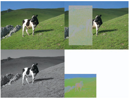
Figure 6.1 Top left: A low-resolution RGB image used for illustrating the use of chroma subsampling in compressing images. Top right: Reconstructed RGB image, and the difference between original and reconstructed pixels. Bottom left: Luminance of the original image. Bottom right: Half-resolution chroma Image. (Image courtesy of Florian Kainz.)

The specifics of converting a red-green-blue or RGB image into luminance and chroma components differ among image file formats. Usually the luminance of an RGB pixel is simply a weighted sum of the pixel’s R, G, and B components. Chroma has two components, one that indicates if the pixel is more red or more green and one that indicates if the pixel is more yellow or more blue. The chroma values contain no luminance information. If two pixels have the same hue and saturation, they have the same chroma values, even if one pixel is brighter than the other (Poynton, 2003, and ITU-R BT.709-3).

Converting an image from RGB to the luminance-chroma format does not directly reduce its size. Both the original and the luminance-chroma image contain three values per pixel. However, since the chroma components contain no luminance information, they can be resized to half their original width and height without noticeably affecting the look of the image. An image consisting of the full-resolution luminance combined with the resized chroma components occupies only half as much space as the original RGB pixels.

Variations of luminance-chroma encoding are a part of practically all image file formats that employ lossy image compression, as well as a part of most digital and analog video formats.

Contrast Masking

If an image contains a boundary between two regions that differ drastically in brightness, then the high contrast between those regions hides low-contrast image features on either side of the boundary. For example, the left image in Figure 6.2 contains two grainy regions that are relatively easy to see against the uniformly gray background and two horizontal lines, one of which is clearly darker than the other.

Figure 6.2 Synthetic test image illustrating the contrast masking exploit in image compression. Note how introducing a much brighter area effectively masks any of the underlying noise and minimizes the differences in the brightness of the two horizontal lines. (Image courtesy of Florian Kainz.)

If the image is overlaid with a white stripe, as shown in the right image in Figure 6.2, then the grainy regions are much harder to distinguish, and it is difficult to tell whether the two horizontal lines have the same brightness or not.

The high-contrast edge between the white stripe and the background hides or masks the presence or absence of nearby low-contrast details. The masking effect is fairly strong in this simple synthetic image, but it is even more effective in photographs and in photoreal computer graphics where object textures, film grain, and digital noise help obscure low-contrast details.

Contrast masking can be exploited for lossy image compression. For example, the image can be split into small 4 × 4-pixel blocks. In each block only the value of the brightest pixel must be stored with high precision; the values of the remaining pixels can be stored with less precision, which requires fewer bits. One such method, with a fixed (and fairly low) compression rate, is described in the extended version of this section (see the Handbook’s website at www.VESHandbookofVFX.com).

Careful observation of the limitations of human vision has led to the discovery of several lossy compression methods that can achieve high compression rates while maintaining excellent image quality, for example, JPEG and JPEG 2000. A technical description of those methods is outside the scope of this section.

File Formats

This subsection presents a listing of image file formats that are typically found in post-production workflows. Due to the complexity of some of the image file formats, not all software packages will implement or support all of the features that are present in the specification of any given format. The listings that follow present information that is typical to most implementations. Where possible, references to the complete definition or specification of the format are given.

Camera RAW File Formats and DNG

RAW image files contain minimally processed data from a digital camera’s sensor. This makes it possible to delay a number of processing decisions, such as setting the white point, noise removal, or color rendering, until full-color images are needed as input to a post-production pipeline.

Unfortunately, even though most RAW files are variations of TIFF there is no common standard in the way data are stored in a file across camera manufacturers and even across different camera models from the same manufacturer. This may limit the long-term viability of data stored in such formats. Common filename extensions include RAW, CR2, CRW, TIF, NEF. The DNG format, also an extension of TIFF, was conceived by Adobe as a way of unifying the various proprietary formats. Adobe has submitted the specification to ISO for possible standardization.

The image sensors in most modern electronic cameras do not record full RGB data for every pixel. Cameras typically use sensors that are equipped with color filter arrays. Each pixel in such a sensor is covered with a red, green, or blue color filter. The filters are arranged in a regular pattern, as per the top example in Figure 6.3.

To reconstruct a full-color picture from an image that has been recorded by such a color filter array sensor, the image is first split into a red, a green, and a blue channel as in the lower diagram in Figure 6.3.

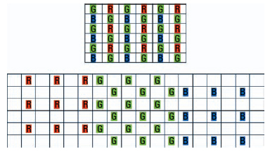
Figure 6.3 Top: Arrangement of pixels in a typical image sensor with a red-green-blue color filter array. Bottom: The interleaved image is separated into three channels; the missing pixels in each channel must be interpolated. (Image courtesy of Piotr Stanczyk.)

Some of the pixels in each channel contain no data. Before combining the red, green, and blue channels into an RGB image, values for the empty pixels in each channel must be interpolated from neighboring pixels that do contain data. This is a non-trivial step and various implementations result in markedly different results.

Owner: Adobe

Extension: DNG

Reference: www.adobe.com/products/dng

Cineon and DPX

DPX is the de facto standard for storing and exchanging digital representations of motion picture film negatives. DPX is defined by an SMPTE standard (ANSI/SMPTE 268M-2003). The format is derived from the image file format originally developed by Kodak for use in its Cineon Digital Film System. The data itself contains a measure of the density of the exposed negative film.

Unfortunately, the standard does not define the exact relationship between light in a depicted scene, code values in the file, and the intended reproduction in a theater. As a result, the exchange of images between production houses requires additional information to avoid ambiguity. Exchange is done largely on an ad hoc basis.

Most frequently, the image data contains three channels representing the red, green, and blue components, each using 10 bits per sample. The DPX standard allows for other data representations including floating point pixels, but this is rarely supported. One of the more useful recent additions to film scanning technology has been the detection of dust particles via an infrared pass. The scanned infrared data can be stored in the alpha channel of a DPX file.

The Cineon and DPX file formats do not provide any mechanisms for data compression so that the size of the image is only dependent on the spatial resolution.

Owner: SMPTE (ANSI/SMPTE268M-2003)

Extension: CIN, DPX

Reference: www.cineon.com/ff_draft.php; http://store.smpte.org

JPEG Image File Format

JPEG is an ubiquitous image file format that is encountered in many workflows. It is the file format of choice when distributing photographic images on the Internet. JPEG compression was developed in the late 1980s. A detailed and accessible description can be found in the book JPEG Still Image Data Compression Standard, by Pennebaker and Mitchell (1993).

JPEG is especially useful in representing images of natural and realistic scenes. DCT compression is very effective at reducing the size of these types of images while maintaining high image fidelity. However, it is not ideal at representing artificial scenes that contain sharp changes in neighboring pixels, say, vector lines or rendered text.

JPEG compression allows the user to trade image quality for compression. Excellent image quality is achieved at compression rates on the order of 15:1. Image quality degrades progressively if file sizes are reduced further, but images remain recognizable even at compression rates on the order of 100:1. Typical JPEG implementations suffer from generational losses and the limitations of 8-bit encoding. Consequently, visual effects production pipelines where images may go through a high number of load-edit-save cycles do not typically employ this format. It is, however, well suited to and used for previewing purposes. It is also used as a starting point for texture painting.

In 2000, JPEG 2000, a successor to the original JPEG compression, was published (ISO/IEC 10918-1:1994). JPEG 2000 achieves higher image quality than the original JPEG at comparable compression rates, and it largely avoids blocky artifacts in highly compressed images. The Digital Cinema Package (DCP), used to distribute digital motion pictures to theaters, employs JPEG 2000 compression, and some digital cameras output JPEG 2000-compressed video, but JPEG 2000 is not commonly used to store intermediate or final images during visual effects production.

Color management for JPEG images via ICC profiles is well established and supported by application software.

Owner: Joint Photographic Experts Group, ISO (ISO/IEC 109181:1994 and 1544-4:2004)

Extension: JPG, JPEG

Reference: www.w3.org/Graphics/JPEG/itu-t81.pdf

OpenEXR

OpenEXR is a format developed by Industrial Light & Magic for use in visual effects production. The software surrounding the reading and writing of OpenEXR files is an open-source project allowing contributions from various sources. OpenEXR is in use in numerous post-production facilities. Its main attractions include 16-bit floating point pixels, lossy and lossless compression, an arbitrary number of channels, support for stereo, and an extensible metadata framework.

Currently, there is no accepted color management standard for OpenEXR, but OpenEXR is tracking the Image Interchange Framework that is being developed by the Academy of Motion Picture Arts and Sciences.

It is important to note that lossy OpenEXR compression rates are not as high as what is possible with JPEG and especially JPEG 2000.

Owner: Open Source

Extension: EXR, SXR (stereo, multi-view)

Reference: www.openexr.com

Photoshop Project Files

Maintained and owned by Adobe for use with the Photoshop software, this format not only represents the image data but the entire state of a Photoshop project including image layers, filters, and other Photoshop specifics. There is also extensive support for working color spaces and color management via ICC profiles.

Initially, the format only supported 8-bit image data, but recent versions have added support for 16-bit integer and 32-bit floating point representations.

Owner: Adobe

Extension: PSD

Reference: www.adobe.com/products/photoshop

Radiance Picture File—HDR

Radiance picture files were developed as an output format for the Radiance ray-tracer, a physically accurate 3D rendering system. Radiance pictures have an extremely large dynamic range and pixel values have an accuracy of about 1%. Radiance pictures contain three channels and each pixel is represented as 4 bytes, resulting in relatively small files sizes. The files can be either uncompressed or run-length encoded.

In digital visual effects, Radiance picture files are most often used when dealing with lighting maps for virtual environments.

Owner: Radiance

Extension: HDR, PIC

Reference: http://radsite.lbl.gov/radiance/refer/filefmts.pdf

Tagged Image File Format (TIFF)

This is a highly flexible image format with a staggering number of variations from binary FAX transmissions to multispectral scientific imaging. The format’s variability can sometimes lead to incompatibilities between file writers and readers, although most implementations do support RGB with an optional alpha channel.

The format is well established and has wide-ranging software support. It is utilized in scientific and medical applications, still photography, printing, and motion picture production. Like JPEG, it has a proven implementation of color management via ICC profiles.

Owner: Adobe

Extension: TIF, TIFF

Reference: http://partners.adobe.com/public/developer/tiff/index.html

References

DPX standard, ANSI/SMPTE 268M-2003 (originally was version 1 268M-1994).

Huffman, D. A. A method for the construction of minimum-redundancy codes. In: Proceedings of the I.R.E. (September 1952) (pp. 1098–1102).

ISO/IEC 1091–:1994. Digital compression and coding of continuous-tone still images: requirements and guidelines.

ISO/IEC 15444-4: 2004. JPEG 2000 image coding system: core coding system.

ITU-R BT.709-3. Parameter values for the HDTV standards for Production and International Programme Exchange.

OpenEXR image format, http://www.openexr.org

Pennebaker, W. B., & Mitchell, J. L. (1993). JPEG still image data compression standard. New York: Springer-Verlag, LLC.

Poynton, C. A. (2003). Digital video and HDTV: algorithms and interfaces.

San Francisco, CA: Morgan Kaufmann Publishers.

Young, T. (1802). On the theory of light and colors. Philosophical Transactions of the Royal Society of London, 92.

4K+ SYSTEMS THEORY BASICS FOR MOTION PICTURE IMAGING

Dr. Hans Kiening

Five years ago digital cameras and cell phones were the biggest thing in consumer electronics, but the most popular phrase today seems to be “HD.” One would think that the “H” in HD stands for “hype.” Although professionals have a clear definition of HD (1920 × 1080 pixels, at least 24 full frames per second, preferably 4:4:4 color resolution), at electronics stores, the “HD-Ready” sticker on hardware offers considerably less performance (1280 × 1024 pixels, 4:2:1, strong compression, etc.). On display are large monitors showing images that are usually interpolated from standard definition images (720 × 576 pixels or less). The catchphrase “HD for the living room” means (on a different quality level)—comparable to the discussion of 2k versus 4k in professional post-production—expectations, and sometimes just basic information, could not be more contradictory. Yet an increasing number of major film projects are already being successfully completed in 4k. So, it’s high time for a technically based appraisal of what is really meant by 2k and 4k. This section strives to make a start.

Part 1: Resolution and Sharpness

To determine resolution, a raster is normally used, employing increasingly fine bars and gaps. A common example in real images would be a picket fence displayed to perspective. In the image of the fence, shown in Figure 6.4, it is evident that the gaps between the boards become increasingly difficult to discriminate as the distance becomes greater. This effect is the basic problem of every optical image. In the foreground of the image, where the boards and gaps haven’t yet been squeezed together by the perspective, a large difference in brightness is recognized. The more the boards and gaps are squeezed together in the distance, the less difference is seen in the brightness.

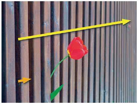
Figure 6.4 Real-world example for a resolution test pattern. (All images courtesy of Dr. Hans Kiening.)

To better understand this effect, the brightness values are shown along the yellow arrow into an x/y diagram (Figure 6.5). The brightness difference seen in the y-axis is called contrast. The curve itself functions like a harmonic oscillation; because the brightness does not change over time but spatially from left to right, the x-axis is called spatial frequency.

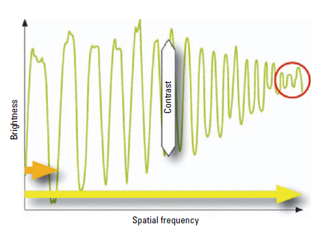
Figure 6.5 Brightness along the picket fence in Figure 6.4.

The distance can be measured from board to board (orange arrow) on an exposed image such as a 35mm. It describes exactly one period in the brightness diagram (Figure 6.5). If such a period in the film image continues, for example, over 0.1mm, then there is a spatial frequency of 10 line pairs/mm (10 lp/mm, 10 cycles/mm, or 10 periods/mm). Visually expressed, a line pair always consists of a bar and a “gap.” It can be clearly seen in Figure 6.4 that the finer the reproduced structure, the more the contrast will be smeared on that point in the image. The limit of the resolution has been reached when one can no longer clearly differentiate between the structures. This means the resolution limit (red circle indicated in Figure 6.5) lies at the spatial frequency where there is just enough contrast left to clearly differentiate between board and gap.

Constructing the Test

Using picket fences as an example (Figure 6.4), the resolution can be described only in one direction. Internationally and scientifically, a system of standardized test images and line pair rasters to determine and analyze resolution has been agreed on. Horizontal and vertical rasters are thereby distributed over the image surface.

To carry out such a test with a film camera, the setup displayed in Figure 6.6 was used. The transparent test pattern was exposed with 25 fps and developed. Figure 6.8 shows the view through a microscope at the image center (orange border in Figure 6.7).

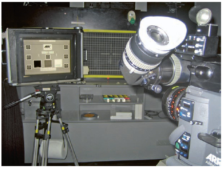
Figure 6.6 Setup for resolution.

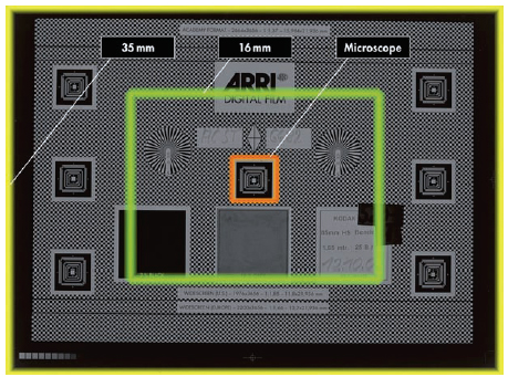
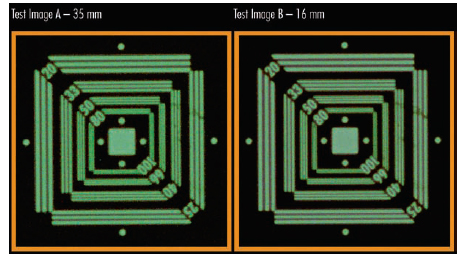
Figure 6.8 View through the microscope at the negative (center).

Resolution Limit 35mm

Camera: ARRICAM ST

Film: Eastman EXR 50D Color Negative Film 5245 EI 50

Lens: HS 85mm F2.8

Distance: 1.65 m

It is apparent that the finest spatial frequency that can still be differentiated lies between 80 and 100 lp/mm. For these calculations, a limit of 80 lp/mm can be assumed. The smallest discernible difference was determined by the following:

1mm/80 1p = 0.012mm/1p

Lines and gaps are equally wide, ergo:

0.012mm/2 = 0.006mm for the smallest detail

Resolution Limit 16mm

Camera: 416

Film: Eastman EXR 50D Color Negative Film 5245 EI 50

Lens: HS 85mm F2.8

Distance: 1.65 m

If a 35mm camera is substituted for a 16mm camera with all other parameters remaining the same (distance, lens), an image will result that is only half the size of the 35mm test image but resolves exactly the same details in the negative.

Results

This test is admittedly an ideal case, but the ideal is the goal when testing the limits of image storage in film. In the test, the smallest resolvable detail is 0.006mm large on the film, whether 35mm or 16mm. Thus, across the full film width there are 24.576mm/0.006 = 4096 details or points for 35mm film and 12.35mm/0.006 = 2048 points for 16mm film. Because this happens in the analog world, these are referred to as points rather than pixels. These statements depend on the following: (1) looking at the center of the image; (2) the film sensitivity is not over 250 ASA; (3) exposure and development are correct; (4) focus is correct; (5) lens and film don’t move against one another during exposure; and; (6) speed <50 fps.

Digital

The same preconditions would also exist for digital cameras (if there were a true 4k resolution camera on the market today); only the negative processing would be omitted. Thus in principle, this test is also suitable for evaluating digital cameras. In that case, however, the test rasters should flow not only horizontally and vertically, but also diagonally and, ideally, circularly. The pixel alignment on the digital camera sensor (Bayer pattern) is rectangular in rows and columns. This allows good reproduction of details, which lie in the exact same direction, but not of diagonal structures, or other details that deviate from the vertical or horizontal. This plays no role in film, because the sensor elements—film grain—are distributed randomly and react equally good or bad in all directions.

Sharpness

Are resolution and sharpness the same? By looking at the images shown in Figure 6.9, one can quickly determine which image is sharper. Although the image on the left comprises twice as many pixels, the image on the right, whose contrast at coarse details is increased with a filter, looks at first glance to be distinctly sharper.

Figure 6.9 Resolution = Sharpness?

The resolution limit describes how much information makes up each image, but not how a person evaluates this information. Fine details such as the picket fence in the distance are irrelevant to a person’s perception of sharpness—a statement that can be easily misunderstood. The human eye, in fact, is able to resolve extremely fine details. This ability is also valid for objects at a greater distance. The decisive physiological point, however, is that fine details do not contribute to the subjective perception of sharpness. Therefore, it’s important to clearly separate the two terms, resolution and sharpness.

The coarse, contour-defining details of an image are most important in determining the perception of sharpness. The sharpness of an image is evaluated when the coarse details are shown in high contrast. A plausible reason can be found in the evolution theory: “A monkey who jumped around in the tops of trees, but who had no conception of distance and strength of a branch, was a dead monkey, and for this reason couldn’t have been one of our ancestors,” said the paleontologist and zoologist George Gaylord Simpson (2008). It wasn’t the small, fine branches that were important to survival, but rather the branch that was strong enough to support the monkey.

Modulation Transfer Function

The term modulation transfer function (MTF) describes the relationship between resolution and sharpness and is the basis for a scientific confirmation of the phenomenon described earlier. The modulation component in MTF means approximately the same as contrast. Evaluate the contrast (modulation) not only where the resolution reaches its limit, but over as many spatial frequencies as possible and connect these points with a curve, to arrive at the so-called MTF (Figure 6.10).

In Figure 6.10, the x-axis illustrates the already established spatial frequency expressed in line pairs per millimeter on the y-axis, instead of the brightness seen in modulation. A modulation of 1 (or 100%) is the ratio of the brightness of a completely white image to the brightness of a completely black image. The higher the spatial frequency (i.e., the finer the structures in the image), the lower the transferred modulation. The curve seen here shows the MTF of the film image seen in Figure 6.8 (35mm). The film’s resolution limit of 80 lp/mm (detail size 0.006mm) has a modulation of approximately 20%.

In the 1970s, Erich Heynacher from Zeiss provided the decisive proof that humans attach more value to coarse, contour-defining details than to fine details when evaluating an image. He found that the area below the MTF curve corresponds to the impression of sharpness perceived by the human eye (the so-called Heynacher integral) (Heynacher, 1963). Expressed simply, the larger the area, the higher the perception of sharpness. It is easy to see that the coarse spatial frequencies make up the largest area of the MTF. The farther right into the image’s finer details, the smaller the area of the MTF. Looking at the camera example in Figure 6.9, it is obvious that the red MTF curve shown in Figure 6.11 frames a larger area than the blue MTF curve, even if it shows twice the resolution.

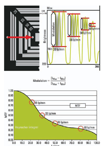
Figure 6.10 Modulation transfer function and the Heynacher integral.

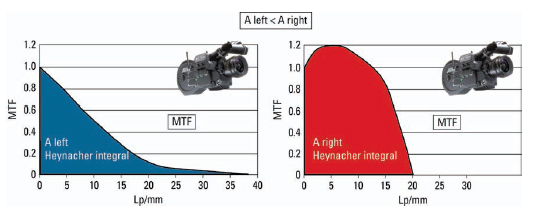
Figure 6.11 MTF and Heynacher integral for Figure 6.10.

For Experts

An explanation of the difference between sine-shaped (MTF) and rectangular (CTF) brightness distribution in such test patterns will not be offered here. However, all relevant MTF curves have been measured according to ISO standards for the fast Fourier transform (FFT of slanted edges).

Part 1 Summary

Sharpness does not depend only on resolution. The modulation at lower spatial frequencies is essential. In other words, contrast in coarse details is significantly more important for the impression of sharpness than contrast at the resolution limit. The resolution that delivers sufficient modulation (20%) in 16mm and 35mm film is reached at a detail size of 0.006mm, which corresponds to a spatial frequency of 80 lp/mm (not the resolution limit <10%).

Part 2: Into the Digital Realm

How large is the storage capacity of the film negative? How many pixels does one need to transfer this spatial information as completely as possible into the digital realm, and what are the prerequisites for a 4k chain of production? These are some of the questions addressed in this section.

The analyses here are deliberately limited to the criteria of resolution, sharpness, and local information content. These, of course, are not the only parameters that determine image quality, but the notion of 4k is usually associated with them.

Film as a Carrier of Information

Film material always possesses the same performance data: the smallest reproducible detail (20% modulation) on a camera film negative (up to EI 200) is about 0.006mm, as determined by the analysis done earlier in this section. This can also be considered the size of film’s pixels, a concept that is well known from electronic image processing. It does not matter if the film is 16mm, 35mm, or 65mm—the crystalline structure of the emulsion is independent of the film format. Also, the transmission capability of the imaging lens is generally high enough to transfer this spatial frequency (0.006mm = 80 lp/mm) almost equally well for all film formats.

The film format becomes relevant, however, when it comes to how many small details are to be stored on its surface—that is the question of the total available storage capacity. In Table 6.1, the number of pixels is indicated for the image’s width and height. Based on the smallest reproducible detail of 0.006mm, Table 6.1 gives an overview of the storage capacity of different film formats.

Scanning

These analog image pixels must now be transferred to the digital realm. Using a Super 35mm image as an example, the situation is as follows:

The maximum information depth is achieved with a line grid of 80 lp/mm. The largest spatial frequency in the film image is therefore 1/0.012mm (line 0.006mm + gap 0.006mm). According to the scanning theorem of Nyquist and Shannon, the digital grid then has to be at least twice as fine, that is, 0.012mm/2 = 0.006mm. Converted to the width of the Super 35mm negative, this adds up to 24.92mm/0.006mm = 4153 pixels for digitization.

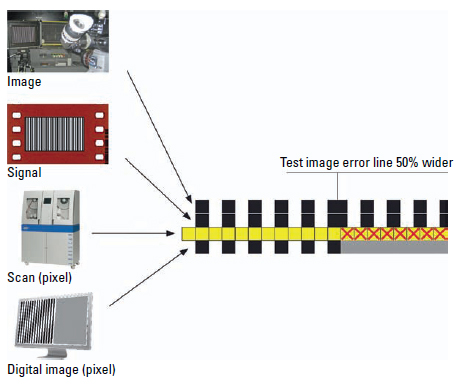
Figure 6.12 Principle of aliasing.

Aliasing

Stick with the line grid as a test image and assume a small error has crept in. One of the lines is 50% wider than all of the others. While the film negative reproduces the test grid unperturbedly and thereby true to the original, the regular digital grid delivers a uniform gray area, starting at the faulty line—simply because the pixels, which are marked with an “x,” consist of half a black line and half a white gap, so the digital grid perceives a simple mix— which is gray.

Figure 6.13 Frequency sweep.

So if the sample to be transferred consists of spatial frequencies that become increasingly higher—as in Figure 6.13—the digital image suddenly shows lines and gaps in the wrong intervals and sizes. This is a physical effect whose manifestations are also known as acoustics in the printing industry. There, the terms beating waves and moiré are in use. In digitization technology, the umbrella term for this is aliasing. Aliasing appears whenever there are regular structures in the images that are of similar size and aligned in the same way as the scanning grid. Its different manifestations are shown in Figure 6.14. The advantage of the film pixels, the grains, is that they are statistically distributed and not aligned to a regular grid and they are different from frame to frame.

Figure 6.14 Aliasing

Figure 6.14 shows an area of incipient destructive interference and an area of pseudo-modulation. This describes the contrast for details, which lie beyond the threshold frequency and which, in the digital image, are indicated in the wrong place (out of phase) and have the wrong size. This phenomenon does not only apply to test grids—even the jackets of Academy Award winners may fall victim to aliasing (Figures 6.15 and 6.16). Note: You can see from these figures that aliasing is a nasty artifact for still pictures. It becomes significantly worse for motion picture because it changes dynamically from frame to frame.

Figure 6.15 Digital still camera with 2 megapixels.

Figure 6.16 Digital still camera with 1 megapixels.

Impact on the MTF

It is very obvious that the aliasing effect also has an impact on the MTF. Pseudo-modulation manifests itself as a renewed rise (hump) in the modulation beyond the scanning limit Pseudo, because the resulting spatial frequencies (lines and gaps) have nothing to do with reality: Instead of becoming finer, as they do in the scene, they actually become wider again in the output image (Figures 6.17 and 6.18).

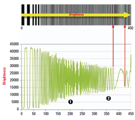
Figure 6.17 Luminance along the frequency sweep.

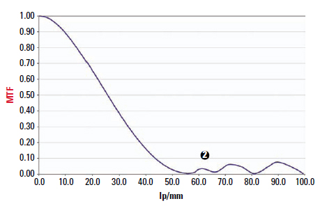
Figure 6.18 Resulting MTF.

Avoiding Alias

The only method for avoiding aliasing is to physically prevent high spatial frequencies from reaching the scanning raster; that is, by defocusing or through a so-called optical low pass, which in principle does the same in a more controlled fashion. Unfortunately, this not only suppresses high spatial frequencies; it also affects the contrast of coarse detail, which is important for sharpness perception.

Another alternative is to use a higher scanning rate with more pixels, but this also has its disadvantages. Because the area of a sensor cannot become unlimitedly large, the single sensor elements have to become smaller to increase the resolution. However, the smaller the area of a sensor element becomes, the less sensitive it will be. Accordingly, the acquired signal must be amplified again, which leads to higher noise and again to limited picture quality. The best solution often lies somewhere in between. A combination of a 3k sensor area (large pixels, little noise) and the use of mechanical microscanning to increase resolution (doubling it to 6k) is the best solution to the problem.

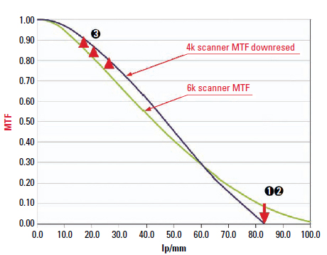
Figure 6.19 Scanner MTF

The currently common maximum resolution in postproduction is 4k. The gained 6k data is calculated down with the help of a filter. In the process, the MTF is changed; thus:

(1) The response at half of the 4k scanning frequency itself is zero.

(2) Spatial frequencies beyond the scanning frequency are suppressed.

(3) The modulation at low spatial frequencies is increased.

Whereas measures (1) and (2) help to avoid aliasing artifacts in an image, measure (3) serves to increase the surface ratio under the MTF. As discussed earlier, this improves the visual impression of sharpness. To transfer the maximum information found in the film negative into the digital realm without aliasing and with as little noise as possible, it is necessary to scan the width of the Super 35mm negative at 6k. This conclusion can be scaled to all other formats.

The Theory of MTF Cascading

What losses actually occur over the course of the digital, analog, or hybrid post-production chain?

The MTF values of the individual chain elements can be multiplied to give the system MTF. With the help of two or more MTF curves one can quickly compare—above all—without any subjectively influenced evaluation. Also, once the MTF of the individual links of the production chain is determined, the expected result can be easily computed at every location within the chain, through simple multiplication of the MTF curves.

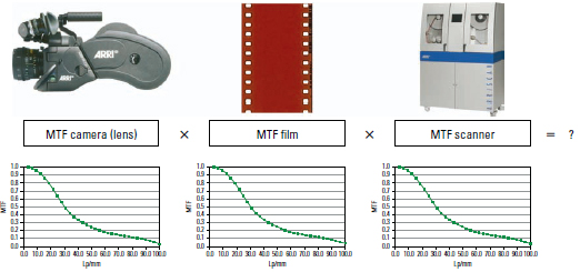
Figure 6.20 Theory of MTF cascading.

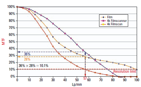
Figure 6.21 Resulting MTF in a 4k scan.

MTF Camera (Lens) × MTF Film × MTF Scanner = ?

An absolutely permissible method for a first estimate is the use of manufacturers’ MTF data for multiplication. However, it must be remarked that there usually are very optimistic numbers behind this data and calculating them in this way shows the best-case scenario. Actual measured values are used for the calculations here. Instead of using the MTF of the raw stock and multiplying it by the MTF of the camera lens, the resulting MTF of the exposed image is directly measured and multiplied by the MTF of a 4k scanner.

What Does the Result Show?

The MTF of a 35mm negative scanned with 4k contains only little more than 56 lp/mm (the equivalent of 3k with the image width of Super 35mm) usable modulation. The resolution limit is defined by the spatial frequency, which is still transferred with 10% modulation. This result computes from the multiplication of the modulation of the scanner and of the film material for 57 lp/mm:

MTF_4k_scanner (57 1p/mm) × MTF_exposed_film (57 1p/mm) = MTF_in_4k_scan (57 1p/mm) 36% × 28% = 10.08%

The same goes for a digital camera with a 4k chip. There, a low-pass filter (actually a deliberate defocusing) must take care of pushing down modulation at half of the sampling frequency (80 lp/mm) to 0, because otherwise aliasing artifacts would occur.

Ultimately, neither a 4k scan nor a (three-chip) 4k camera sensor can really transfer resolution up to 4k.

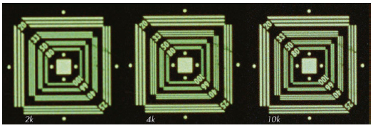
Figure 6.22 From left, 2k, 4k, and 10k scans of the same 35mm camera negative.

This is a not an easily digestible paradigm. It basically means that 4k data only contains 4k information if it was created pixel by pixel on a computer—without creating an optical image beforehand. However, this cannot be the solution, because then in the future there would be animated movies only—a scenario in which actors and their affairs could only be created on the computer. This would be a tragic loss and not just for supermarket tabloid newspapers!

Part 2 Summary

In the foreseeable future, 4k projectors will be available, but their full quality will come into its own only when the input data provides this resolution without loss. At the moment, a correctly exposed and 6k/4k scanned 35mm film negative is the only practically existing acquisition medium for moving pictures that comes close to this requirement. By viewing from a different angle one could say that the 4k projection technology will make it possible to see the quality of 35mm negatives without incurring losses through analog processing laboratory technology. The limiting factor in the digital intermediate (DI) workflow is not the (ideal exposed) 35mm film but the 4k digitization. As you can see in Figure 6.22, a gain in sharpness is still possible when switching to higher resolutions. Now imagine how much more image quality could be achieved with 65mm (factor 2.6 more information than 35mm)!

These statements are all based on the status quo in the film technology—for an outlook on the potential of tomorrow’s film characteristics read Tadaaki Tani’s article (Tani, 2007). The bottom line is that 35mm film stores enough information reserves for digitization with 4k+.

Part 3: Does 4k Look Better Than 2k?

The two most frequently asked questions regarding this subject are “How much quality is lost in the analog and the DI chain?” and “Is 2k resolution high enough for the digital intermediate workflow?”

The Analog Process

“An analog copy is always worse than the original.” This is an often-repeated assertion. But it is true only to a certain extent in the classic post-production process; there are in fact quality-determining parameters that, if controlled carefully enough, can ensure that the level of quality is maintained: When photometric requirements are upheld throughout the chain of image capture, creating the intermediates and printing, the desired brightness and color information can be preserved for all intents and purposes.

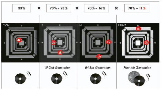
Figure 6.23 10k scans (green), photochemical lab from camera negative to print.

Clear loss of quality, however, indeed occurs where structures, that is, spatial image information, are transferred. In other words, resolution and sharpness are reduced. This occurs as a result of the rules of multiplication. Table 6.3 shows how 50 lp/mm with a native 33% modulation in the original is transferred throughout the process.

This, however, is an idealized formula, because it assumes that the modulation of the film material and the contact printing show no loss of quality. This is not the case in reality, which can be seen in the differences between the horizontal and vertical resolutions.

Is 2k Enough for the DI Workflow?

Although the word digital suggests a digital reproduction with zero loss of quality, the DI process is bound by the same rules that apply to the analog process because analog components (i.e., optical path of scanner and recorder) are incorporated. To make this clearer, again perform the simple multiplication of the MTF resolution limit in 4k (= 80 lp/mm). The MTF data illustrate the best filming and DI components that can be currently achieved.

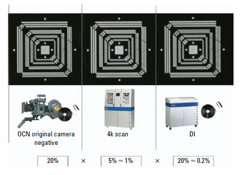
Figure 6.24 DI workflow.

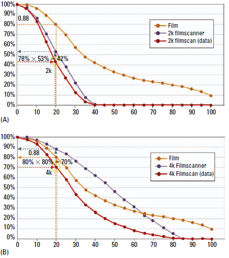
Figure 6.25 (A) 2k scan. (B) 4k scan.

As the multiplication proves, inherent to the 4k DI chain, modulation cannot occur at 80 lp/mm, even though the digitally exposed internegative shows considerably more image information than can be preserved throughout the traditional analog chain. An internegative, or intermediate negative, is a film stock used to duplicate an original camera negative. Conventionally it is generated with film printers alternatively exposed from the digitized data on a film recorder. Then it is called a digital intermediate.

Why, then, is a 4k digital process still a good idea, even though it cannot reproduce full 4k image information? The answer is simple, according to the Heynacher integral (the area beneath the MTF curve): The perception of sharpness depends on the modulation of coarse local frequencies. When these are transferred with a higher modulation, the image is perceived as sharp. Figure 6.26 shows the results of a 2k and 4k scan.

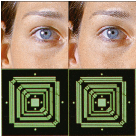
Figure 6.26 Cutout of a 2k (left) and a 4k (right) digital internegative.

Because a 4k scanner offers not only more resolution but also more modulation in lower local frequencies, the resulting 4k images will be perceived as being sharper. When this data is recorded out in 4k on Fuji RDI, for example, it produces the results shown in Figure 6.24.

Part 3 Summary

A 4k workflow is advantageous for DI and film archiving. The MTF characteristics seen in 4k scanning will transfer coarse detail (which determines the perception of sharpness) with much more contrast than 2k scanning. It is thereby irrelevant whether or not the resolution limit of the source material is resolved. It is very important for the available frequency spectrum to be transferred with as little loss as possible.

Part 4: Visual Perception Limitations for Large Screens

The section discusses the most important step in the production chain—the human eye. Again, the focus is resolution, sharpness, and alias. More specifically, the focus is now on general perception at the limits of human visual systems, when viewing large images on the screen. This limitation shows how much effort one should put into digitization of detail.

A very common rumor still circulates that alleges that one could simply forget about all the effort of 4k, because nobody can see it on the screen anyway. The next sections take a closer look to see if this is really true!

Basic Parameters

Three simple concepts can be used to describe what is important for a natural and sharp image, listed here in a descending order of importance:

(1)   Image information is not compromised with alias artifacts.

(2)   Low spatial frequencies show high modulation.

(3)   High spatial frequencies are still visible.

This implicitly means that an alias-affected image is much more annoying than one with pure resolution.

Further, it would be completely wrong to conclude that one could generate a naturally sharp image by using low resolution and just push it with a filter. Alias-free images and high sharpness can be reached only if oversampling and the right filters for downscaling to the final format have been used.

Resolution of the Human Eye

The fovea of the human eye (the part of the retina that is responsible for sharp central vision) includes about 140,000 sensor cells per square millimeter. This means that if two objects are projected with a separation distance of more than 4 m on the fovea, a human with normal visual acuity (20/20) can resolve them. On the object side, this corresponds to 0.2mm in a distance of 1 m (or 1 minute of arc).

In practice, of course, this depends on whether the viewer is concentrating only on the center of the viewing field, whether the object is moving very slowly or not at all, and whether the object has good contrast to the background.

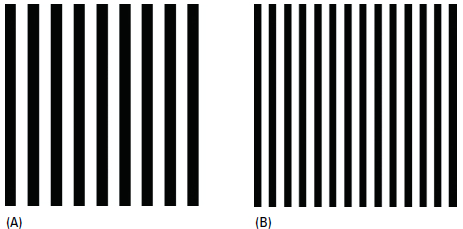
Figure 6.27 (A) 3mm (to be viewed at a 10-m distance). (B) 2mm.

As discussed previously, the actual resolution limit will not be used for further discussion but rather the detail size that can be clearly seen. Allowing for some amount of tolerance, this would be around 0.3mm at a 1-m distance (= 1.03 minutes of arc). In a certain range, one can assume a linear relation between distance and the detail size:

0.3mm in 1 – m distance » 3mm in 10 – m distance

This hypothesis can be easily proved. Pin the test pattern displayed in Figure 6.27A and B on a well-lit wall and walk away 10 m. You should be able to clearly differentiate between the lines and gaps in Figure 6.27A (3mm); in Figure 6.27B (2mm), however, the difference is barely seen. Of course, this requires an ideal visual acuity of 20/20. Nevertheless, if you can’t resolve the pattern in Figure 6.27A, you might consider paying a visit to an ophthalmologist!

Large-Screen Projection

This experiment can be transferred for the conditions in a theater. Figure 6.28 shows the outline of a cinema with approximately 400 seats and a screen width of 12 m. The center row of the audience is at 10 m. An observer in this row would look at the screen with a viewing angle of 60 degrees. Assuming that the projection in this theater is digital, the observer could easily differentiate 12,000mm/3mm = 4000 pixels.

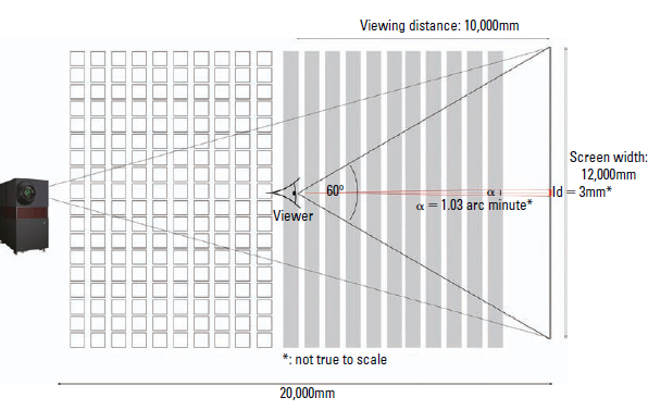
Figure 6.28 Resolution limit in the theater.

The resolution limit is not reached below a distance of 14 m. In other words, under these conditions more than 50% of the audience would see image detail up to the highest spatial frequency of the projector.

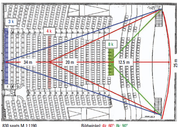
Figure 6.29 Resolution limit for large screens.

Large theaters generally have screens with widths of 25 m or more. Figure 6.29 shows the number of pixels per image width that would be needed if the resolution limit of the eye were the critical parameter for dimensioning a digital projection.

Part 4 Summary

It can be concluded that the rumor is simply not true! A large portion of the audience would be able to see the 4k resolution of the projector. At the same time, the higher resolution inevitably raises the modulation of lower spatial frequencies, which in turn benefits everyone in the theater.

Conclusion

The discussions in this section have shown that a scientific approach is necessary to get a clear view of the real problem instead of merely counting megapixels. This section has addressed only the static image quality factors: sharpness and resolution. As mentioned at the start of this section, there are many more parameters to consider; therefore, an article about the transfer of photometry (sensitivity, contrast, characteristic curve) from scene to screen is being written.

References

Heynacher, E. (1963). Objective image quality criteria based on transformation theory with a subjective scale, Oberkochen, Germany. Zeiss-Mitteilungen, 3(1).

Simpson, G. <http://de.wikipedia.org/wiki/George_Gaylord_Simpson>. Accessed January 2008.

Tani, T. (2007). AgX photography: present and future. Journal of Imaging Science and Technology, 51(2), 110–116.

FILM SCANNING AND RECORDING

Charles Finance

Scanning

Scanning is the process by which the analog image that is visible on film (that is, what one considers as a traditional image composed of continuous tones of gray and infinitely varying colors) is converted into a digital file of zeros and ones. Every filmed element must first be scanned and converted to a digital format before it can be worked on in a computer.⁹

The fundamental function of every scanner is to produce a faithful digital replica of the filmed image. In doing so, scanners must deal with and reproduce the negative’s resolution, dynamic range, density, and color. In scanning, the analog film image is converted to a digital file and stored in one of several formats. Common formats in use today are Cineon (developed by Kodak), DPX (Digital Picture Exchange), and TIFF (Tagged Image File Format). These formats are favored because they preserve the original raw image data of the film.

When scanning with raw image data formatting, as much of the original data as possible is captured and stored by the scanning device. By extension one can easily recognize that the scanning device’s limitations will have a severe impact on the information that is captured. Therefore it is essential to have at least a passing understanding of scanning and the options available. And it is equally essential that tests be performed before one commits an entire project to a specific scanning company.

A scanner is comprised of several key elements: a film transport system, a light source, a digital sensor, electronics that convert the image to zeros and ones, a user interface (usually a computer workstation), and a storage device. That storage device—normally an array of hard drives—is not necessarily part of the scanning system but is nonetheless still important.

During scanning, film is moved past the scanner’s light source and digital sensor, or light detector. Current scanners take two different approaches to how film is transported during scanning. In some models the film moves past the scanning aperture in a continuous path (continuous-scan). These types of scanners are descendants of earlier telecine technology that evolved primarily in television. The other type of scanner uses an intermittent pull-down in which the film is pulled down one frame at a time and is momentarily locked in place by register pins in the aperture as the image is scanned. These scanners are descendants of film technology.

Scans must have maximum image stability. The best scanning systems achieve image stability by pin-registering the film as it is scanned, similar to pin-registered cameras. Other scanning systems attempt to stabilize the image through utilization of optical registering. This is a system in which the sprockets of the film are measured optically and the image is digitally registered frame by frame to match the previous frame’s sprockets. In spite of repeated attempts by manufacturers to produce truly stable images, these types of systems are not satisfactory for visual effects work because they cannot, at present, provide the reliably stable images necessary for critical effects shots. By paying close attention to the stability of the image at the scanning stage, one can hopefully begin the visual effects work without performing further stabilization of the image.¹⁰

Engineers have developed several methods for converting an analog image into streams of digital data. The details of that process are beyond the scope of this book. In each method, the scanner looks at almost 2.5 million points on a standard Academy 35mm frame, detects the color and luminance value of the light at each point, and converts that into a packet of digital data. This is accomplished by using a line array, frame array, or spot sampler type of digital sensor or chip.

Resolution

Of great importance to the visual effects practitioner is resolution. Scanning can be done at various resolutions, but as of this writing 2k is the most common. In a 2k scan the digital sensor reads the color and density of approximately 2000 points horizontally across the width of a full 35mm frame, and approximately 1500 points vertically.¹¹ This resolution has been found to be satisfactory for standard film projection in movie theaters.

Resolution of 4k is rapidly becoming more common in 35mm film work as the technology continues to improve. This represents not just a doubling, but effectively a quadrupling of the resolution over 2k. Scanning in 4k and then downsizing the resolution to 2k before the visual effects work is begun has also become an increasingly standard practice. Many VFX Supervisors and scanning scientists agree that “A superior scan requires a superior resolution source, generally twice that of the working resolution. For example, if a true 2k image is desired, then the scan has to be derived from a 4k scan and scaled down to the 2k image. This technique produces a superior scan more suitable for digital work.”¹² It takes a fairly educated eye to tell the difference, but many leaders in the industry feel that even average viewers may be subliminally sensitive to the difference between 2k and 4k resolution.

Higher levels of resolutions of scanning are possible, and 65mm, IMAX, and other special-venue film formats usually employ 6k, 8k, and even higher resolutions. It is important to recognize that resolution is a term that is often misunderstood. For example, 4k on a 35mm frame is effectively a higher resolution than 4k on an IMAX frame. For a better understanding of the term and its ramifications, please see the preceding section on resolution and perceived sharpness of an image.

Storage

The scanning of film results in digital data. That data must be stored as it is scanned and then archived for later use. Usually, the scans are stored on large active hard drives on site and then backed up and also transferred to another storage medium that the client uses. Until recently this would have been onto several commonly used digital tape formats: DLT, DTF, Metrum, or Exabyte. The choice differed according to the tape drives that were being used by different digital facilities and their clients. However, like so much else in the industry, advancing technology has made these forms of digital storage obsolete. Today, data from digital scans are stored on portable or external hard drives or flash memory. From there, the data can be distributed to their end users, including visual effects facilities, on physical media or via secured Internet connections.

Estimating the Cost of Scanning

On most visual effects-heavy shows, a VFX Producer will have prepared a digital shot breakdown that lists the number of layers (meaning filmed elements) that need to be scanned. Since scanning costs are charged by the frame, it is essential to know how many layers are needed in each shot and the length in frames of each layer. Obviously, there is no way to know the exact number until the shot is filmed, edited, and sometimes temp or rough-comped together. To get around this dilemma in pre-production, VFX Producers use an industry-wide rule of thumb that assumes that a shot runs 5 seconds, or 120 frames (based on 24 fps). Experienced VFX Producers and Supervisors may also budget for an extra scan layer for each shot as a contingency because of the frequent changes that occur on set.

To the customary 120-frame length of a shot a handle is added, which is generally a minimum of 8 frames at the head and tail of each element or plate, for a total of 16 frames (though handles may be longer or shorter). As with all services, scanning costs vary and are negotiable. At the time of this writing, scanning services ranged from $0.45 to $0.55 per frame, and they may well continue to drift lower as the technology improves and competition from image capture by digital cameras becomes more common.

To gain an appreciation of how rapidly these costs can escalate, assume that there are 200 live-action plates to be scanned running an average of 5 seconds each, plus 16 frames of handle, for a total of 136 frames per layer. At $0.50 per frame, the scanning costs come to $13,600.

Be aware that most scanning facilities will charge a setup fee. These basically pay for a line-up person to take the negative supplied by production and prepare it for scanning. There is a certain amount of labor involved, and it is a delicate task since the lineup person must handle the original negative. As a general rule, the negative of several shots should be grouped together and sent to the scanning facility in batches. The number of setups, therefore, will be a fraction of the number of scan layers.

Recording

Recording—putting the digital image back on film—is currently the final step in the process of creating a visual effects shot.¹³ This is where the digital file that represents each frame of an effects shot is converted from the digital into the analog (film) medium. In other words, it goes from a computer (which “thinks” in zeros and ones) back out to film (which is an actual image that is projected). Normally, the digital files are output to a new negative, which is then cut into the negative of the completed show.

Images are recorded out for a number of applications:

•   delivery of visual effects shots,

•   digital intermediates,

•   HD-acquired productions,

•   digital trailers,

•   tape-to-film transfer,

•   archive to film,

•   digital film restoration, and

•   long-form 65mm productions.

Approaches to Recording Out

Two technologically distinct approaches are used for recording digital files to film. In one method, the final images are photographed off a high-quality cathode-ray tube (CRT) not unlike the picture tube in a TV set but far superior in resolution. In the other, a laser beam is used to expose the film. Both methods result in a new negative that is cut into the completed show’s negative.

Film-Out Requirements

A good film-out must meet the highest standards of the following critical qualities:

•   Resolution: A measure of the sharpness of an image or of the fineness with which a device (such as a video display, printer, or scanner) can produce or record such an image, usually expressed as the total number or density of pixels in the image (e.g., a resolution of 1200 dots per inch).¹⁴

•   Dynamic range: Visually speaking, the film, charge-coupled device (CCD), or sensor’s ability to hold the brightest point to the darkest point. This ability, or range, is usually expressed as a curve. The distance between the highest and the lowest points and how smooth that curve is connecting the two visually demonstrates the dynamic range of the film or device.

•   Color fidelity: The successful interoperability of color data, from image creation or capture to output across multiple media such as film, broadcast, DVD, etc., such that the color reproduction quality remains consistent throughout.

Both recording technologies—CRT and laser based—have their advocates. Of the two methods, laser-based recording is now widely recognized as yielding better results for 35mm theatrical projects. However, it should be noted that recording from CRT is still used extensively for large-format films, such as IMAX, because a CRT tube offers a larger target from which to record.

It is good practice to test film-out technologies across several different facilities, using the same negative before choosing a facility to execute the work. The differences among facilities can be significant.

Estimating the Cost of Recording

As with scanning, recording is charged by the frame. On average, record-out costs tend to be slightly higher than scanning, but can also be negotiated to $0.65 to $0.75 or less, especially if a high volume of work can be guaranteed to a facility.

To continue with the previous example, assume that the number of visual effects shots that actually ends up in a movie is 100, each averaging 5 seconds for a total of 12,000 frames to be recorded out to film. To estimate record-out costs under this scenario, one would apply the formula of number of shots (100 in the example) × 120 (the number of assumed frames) × cost per frame. At a median price of $0.70/frame, recording costs would come to $8,400.

Whereas scanning is usually acceptable on the first try, that is not the case with recording or filming out. Visual effects shots typically have to be recorded two or three times before they are deemed acceptable (and that’s not counting the tests a facility may record for its own purposes). In large part this is because digital artists view their images on monitors, and no matter how good a monitor is it is extremely difficult—even for a discerning eye—to see tiny flaws that are readily visible when the shot is projected on a theater screen. What is more, a shot may not “cut in” well with the surrounding shots in terms of its color, density, contrast, graininess, and other qualities. So the first record-out may serve more as an opportunity to tweak the shot than as the final accepted version of the shot. Using these common practices, by the time the 100 shots are approved, thousands of additional dollars will have been added to recording costs. And that does not include additional items such as color or resolution tests, rescans, and lab costs.

Ideally one would record out only the exact number of frames of each shot as it appears in the cut. However, in actual practice it has become relatively common for a visual effects facility to be asked to output shots up to 3 feet longer than they are in the cut to give directors and editors the ability to change the cut up to the time of making the digital intermediate.

Most facilities that perform this service will also have a setup charge. As with scanning, finished effects shots are sent to the recording facility in batches whenever possible. But because final composites can sometimes dribble out of a visual effects facility one at a time, it is difficult to guess at a consistent average for the number of shots per batch. Three is probably as good a number as any.

Recorders also should be pin registered. Output is commonly recorded to Eastman 5242 or Fuji intermediate stock. It is best to have the facility do the record-out at the stock’s full dynamic range. Virtually all recorders run at much lower than real-time speed, capable of recording only a few frames per second. Only one system, whose use is confined mainly to Europe for limited film releases, is capable of recording out at real-time speed.

COLOR MANAGEMENT

Joseph Goldstone

Any visual effects professional whose personal contribution is judged on color should read the three guidelines below; anyone building a workflow from scratch or integrating existing workflows should read (or at least skim) this entire section.

The Three Guidelines

1.  Make critical color decisions in the screening room, not in an artist’s cubicle.

2.  At the desktop, use an open-source or commercial color management system if possible, but don’t expect too much.

3.  Understand and document the color image encodings produced by a production’s digital motion picture (DMP) cameras, renderers, and film scanners, and the encodings consumed by displays, film recorders, and digital projectors that deliver production output to clients.

Digital Color Image Encodings and Digital Cameras

Visual effects work now includes a bewildering variety of image representations: 10-bit log scanner output, 8-bit display-ready images baked for sRGB monitors, Adobe RGB-encoded wide-gamut reference plates from still cameras, and now raw (sometimes inappropriately termed log) data from digital motion picture cameras. The best way to compare two image encodings (encoding encompasses not just the image bits but their meaning and expected viewing environment as well) is to map them onto the same standard conceptual framework.

Compared here are two color image encodings usually available from high-end digital single lens reflex (DSLR) still cameras: a well-defined display-ready Adobe RGB image encoding and a less-well-defined camera raw image encoding. This situation closely parallels the traditional HD and raw image encodings employed by digital cameras from Panavision, ARRI, Thomson, Red, and other manufacturers. The terminology in Figure 6.30 will be explained as these two image encodings are discussed.

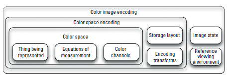
Figure 6.30 Conceptual color image encoding hierarchy. (Image courtesy of Joseph Goldstone.)

At the lowest level—and in the diagram’s innermost boxes— Adobe RGB’s color space is defined¹⁵ to represent colors as they would be measured by some physical device.¹⁶ Measured colors, with the measurement results expressed in terms of what are termed the CIE X, Y, and Z primaries (described in detail shortly), can be converted to corresponding amounts of Adobe RGB’s R, G, and B primaries by multiplying X, Y, and Z against a 3 × 3 matrix given in the Adobe RGB specification. The RGB values are represented as normalized numbers (i.e., between 0.0 and 1.0).

Adobe RGB’s color space encoding specification provides for two methods of digitally encoding RGB color space values for storage: as unsigned 8-bit integers and as unsigned 16-bit integers. The normalized values are put through a simple power function with exponent 2.19921875, the output of which is scaled to either 0.0 to 255.0 for the unsigned 8-bit integer encoding, or 0.0 to 65535.0 for the unsigned 16-bit integer encoding, and finally the interpolated value is rounded to the nearest whole number and stored in the 8- or 16-bit field.

Finally, Adobe RGB’s color image encoding specifies that the image colors as a whole are those of an image ready for display. Several terms are used to express this idea: Such an image is said to be output-referred or—in an unfortunate collision with an existing visual effects term—such an image is said to be color rendered. Color rendering in the language of color science and color management means the transformation of an image to account for differences in viewing environment. A digital still camera producing JPEG files (typically encoded in either the Adobe RGB color space or sRGB¹⁷) will color render the captured image to account for the difference between, for example, the image subject standing in bright sunlight on a desert mesa, and the image reproduction in a typical office on a monitor whose peak white luminance is hundreds of times less powerful than desert sunlight. Such color rendering is usually performed prior to the quantization and rounding specified by the color space encoding.

Adobe RGB says nothing about how the color rendering was performed; the specification is concerned solely with displayable imagery, and any details of how the displayable image came to be are irrelevant. The details of display, on the other hand, are very relevant: The colors are intended to be viewed on a display with a peak white luminance of 160 cd/m² (roughly 47 foot-lamberts), whose contrast ratio is roughly 290:1, with the white’s chromaticity being that of D65 (roughly the color of overcast daylight), and with the area immediately around the image being a gray of identical chromaticity but with 20% of the luminance of displayed white.

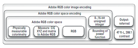
Figure 6.31 Color image encoding hierarchy for Adobe RGB. (Image courtesy of Joseph Goldstone.)

Turning to camera raw formats for digital still and motion picture cameras, Figure 6.32 shows those color image encodings are quite different from that of Adobe RGB.

Like Adobe RGB, the camera raw colors represent physically measurable colors. Unlike Adobe RGB, there is no mandated breakdown into particular image channels; some raw formats used by single-sensor cameras, for example, provide for two green channels if the camera sensor contains twice the number of green-filtered pixels as it does red-filtered and blue-filtered ones.

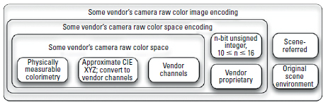
Figure 6.32 Color image encoding hierarchy for camera raw. (Image courtesy of Joseph Goldstone.)

The encoded colors leaving the camera are similarly unconstrained, but typically the encoding provides for three or four channels and the bit depth (not necessarily the same for all channels) ranges between 10 and 16 bits.

With all of this uncertainty it is reasonable to ask why anyone would want camera raw encodings. The answer is that the image data are not color rendered; in color management terms, they are scene referred. If the vendor provides some post-processing tool that converts the image data to a more standard RGB encoding without losing the raw nature of the image data (that is, without color rendering it for some display device), then this scene-referred data may play very well with CGI renderers and compositors. For digital still cameras, Adobe’s DNG Converter and Dave Coffin’s open-source dcraw program can be used to perform this type of extraction. For digital motion picture cameras, there are no such well-publicized, freely available tools at the time of this writing (early 2010), although the input device transforms of the Academy of Motion Picture Arts and Sciences’ Image Interchange Framework (discussed elsewhere in this chapter) will provide this ability when available.

With raw encodings, color rendering will need to be done downstream before the completed shot is shown in a theater. Color rendering is more easily done by the visual effects team, however, than it can be undone if the camera manufacturer has baked in color rendering in a non-raw format.

The color image encoding for camera raw implicitly has as its viewing environment the original scene itself.

CIE XYZ Colorimetry and CIE Chromaticity Coordinates

In introducing Adobe RGB, it was mentioned that Adobe RGB’s definitions of red, green, and blue are provided by mathematical derivation from CIE XYZ values—but what are CIE XYZ values? The psychophysics and mathematics by which colors are specified was worked out in the early 20th century and standardized by the Commission Internationale d’Éclairage (CIE); the most commonly used device-independent metric for colorimetric specification is known as the CIE 1931 Standard Observer, which describes colors in terms of their relative proportions of three primaries: X, Y, and Z (often pronounced “big X,” “big Y,” and “big Z” or “cap X,” “cap Y,” and “cap Z”). These proportions are called a color’s tristimulus values. Any color thus described can be used to derive a second CIE quantity, known as that color’s chromaticity, a measure that expresses the aspects of color disregarding luminance. The usual way to express chromaticity is in terms of chromaticity coordinates × and y (pronounced “little x” and “little y”). The equations relating × and y and X, Y, and Z are shown in Figure 6.33.

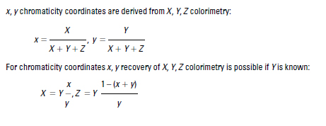
Figure 6.33 Equations relating x, y and X, Y, and Z. (Image courtesy of Joseph Goldstone.)

Commonly Encountered Primaries and White Points

A projection of the chromaticity coordinates of a color space’s primaries onto a 2D plane is often (and misleadingly) used to compare a color space’s coverage of the set of all possible colors. Figure 6.34 gives chromaticity coordinates for primaries and white points of color space data metrics used in visual effects practice. Figure 6.35 shows the primaries projected onto a chromaticity diagram. For a better way to compare color spaces, see Figure 6.36.

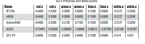
Figure 6.34 Primaries and white points of various encodings. (Image courtesy of Joseph Goldstone.)

Camera Color Analysis Gamuts

The portion of the color space where a camera’s output (or other capture system’s output; scanned film will be described later in this section) distinguishes color variation is sometimes termed its color analysis gamut. For DMP cameras the color analysis gamut is limited by both what the camera sensors can differentiate and by the set of colors the camera output encoding can represent.

RGB Triangles on the Chromaticity Diagram

If a camera were to output CIE XYZ signals, those signals could represent any captured color (since CIE XYZ by definition represents all colors). No commercially available DMP camera outputs XYZ signals, however; usually the color space output encoding is some form of RGB (as RGB, or internally processed to YCbCr). Placing the three BT.709 RGB primaries on a chromaticity diagram (within a vaguely horseshoeshaped boundary representing the spectral locus) makes it clear that many commonly used encoding primaries cannot be combined in positive proportion to represent the full range of colors. (Emergent schemes for wide-gamut color encodings allow RGB weights below zero and above unity but these schemes aren’t yet well standardized, nor therefore widely deployed.)

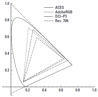
Figure 6.35 Primaries and the set of chromaticities perceived by humans. (Image courtesy of Joseph Goldstone.)

Display Reproduction Gamuts

The counterpart to the camera color analysis gamut is the display reproduction gamut, the set of all colors that a display can reproduce. In an effort to satisfy the needs of the graphic arts industries, desktop monitor manufacturers have expanded the reproduction gamuts of their high-end products considerably in the past few years; today’s best monitors can match all or nearly all of the colors in the reproduction gamut of exhibition-venue commercial digital projection (although high-end projectors in darkened theaters still have a bigger gamut near black because of substantially higher contrast than desktop displays).

This expansion has had the benefit of allowing visual effects artists to see colors at the desktop that previously might have been clipped to the boundary of a smaller (typically sRGB) reproduction gamut volume. On the flip side it means that whereas previously an sRGB-compliant display might have properly reproduced the colors of the encoded image, a wide-gamut display supplied with sRGB-encoded imagery will—in the absence of color management—misinterpret the encoded image. The most common sign of this is when certain memory colors (green grass, for example) are reproduced with extreme oversaturation.

Figure 6.36 compares¹⁸ the reproduction gamut of a laptop monitor with that of a monitor reproducing most of the colors produced by a commercial theatrical venue digital projector. The point is not to denigrate laptop capabilities; it is that reproduction gamut comparisons should be made volumetrically.

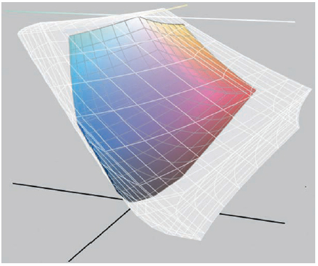
Figure 6.36 Comparison of monitor reproduction gamuts. (Image courtesy of Joseph Goldstone.)

Transcoding versus Color Rerendering

The complexity of transforming color image data optimized for one display into image data optimized for another display will depend, obviously, on the degree of difference between the two. If the displays’ black levels, white luminance, and viewing conditions are identical, and if the displays’ relationships between signal level and output (a display’s gamma) are similarly so, but the primary chromaticities are different, for example, then the encoded colors can be transcoded by linearizing¹⁹ the first display’s encoded RGB values, converting them to CIE XYZ values, converting those CIE XYZ values to the corresponding RGB values for the second display, and reimposing the encoding nonlinearity.²⁰

If the contrast or white levels or viewing conditions are grossly dissimilar, then the best solution is probably color rerendering: Any color rendering implicitly or explicitly done for the first display is undone, and the non-color-rendered CIE XYZ values are color rendered for the second display.

Gamut Clipping, Gamut Warnings, and Gamut Mapping

CG artists frequently use monitors that cannot accurately display image data created by large-gamut capture systems. How this can happen with film will be described shortly, but the particular gamut of film isn’t required to exemplify the problem.

Consider once more a camera producing images encoded in Adobe RGB, which has a more saturated green primary than many other encodings. If that camera captures an image of an extremely green object—one with many different shades of a green so intense they are almost at the limit of what Adobe RGB can represent—and those images are displayed on a DCI-P3-compliant projector, and if the green shades are legal Adobe RGB values falling outside the DCI-P3 gamut, the intense greens may “block up” as the projector reaches its limits in reproducing those shades.

Such gamut clipping is almost always objectionable. The alternatives are to provide some warning when it occurs (for more subtle instances of the problem) or to systematically transform the encoded image data by nonlinearly compressing it into the reproduction gamut in some visually acceptable fashion. Gamut mapping strategies can be quite complex and are outside the scope of this chapter.²¹

Color Management at the Desktop

With the above as background, the responsibilities of any color management system are thus to:

•   Interpret image data according to the image’s associated color image encoding.

•   Provide a path to and from some common color space in which the correctly interpreted captured image data can be combined (a “working space”).

•   Display those original or combined image data as an accurate reproduction of what the final consumer (e.g., moviegoer) will see.

The description of the relationship between capture device code values and some reference colorimetric space is held by what is variously called an input profile, or an input device transform, or some similar nomenclature.

The space in which image data is combined is often based on some form of CIE colorimetry, either CIE XYZ, or a derived space such as CIE LAB (which has the advantage of being more perceptually uniform than CIE XYZ: In the 3D CIE LAB color space, a distance of one unit between any two represented colors means that they are just barely perceptible as different).

The relationship between the encoded image data accepted by digital display devices and the CIE colorimetry that those devices then produce is described by an output profile (or in some systems, an output device transform). Typically this is an analytical or empirical mapping between RGB code values and the resultant displayed CIE XYZ colorimetry; also typically, what is needed is the inverse of this mapping.

If one color renders the colorimetry of the captured, synthesized, or composited scene, the result is CIE XYZ, or some RGB values that can be related to CIE XYZ by a simple 3 × 3 matrix. What needs to be sent to the display device, however, are device code values, so the output device profile must be inverted to get an analytic or empirical mapping from the color-rendered, displayable colorimetry to the device code values that will produce that colorimetry. Note that any color management system doing this will have to deal with the case where the output of the color-rendering algorithm is outside the reproduction gamut of the chosen device; how this is handled tends to be specific to the particular color management system.

The ICC Color Management Architecture

As a first illustration of such systems, consider the color management architecture proposed by the International Color Consortium (ICC). This is the color management system underlying most Adobe products; in addition to proprietary implementations by Adobe, Kodak, Apple, Microsoft, Canon, Sun, etc., there are at least three open-source²² ICC implementations as well.

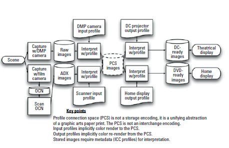
Figure 6.37 Color management using the ICC architecture. (Image courtesy of Joseph Goldstone.)

In the ICC architecture, an input profile defines the mapping of input code values from a capture device into the Profile Connection Space (PCS). The ICC PCS was originally created to meet the needs of the graphic arts industry, but has been used with some success in DMP work. ICC PCS values represent colors ready for printing on a graphic arts press and thus are already color rendered. In Figure 6.37, ICC input profiles map captured image data code values from a digital still camera (DSC) and a digital motion picture camera (DMP) into the PCS. An ICC output profile maps PCS values into digital projector code values, appropriately rerendering the PCS colorimetry for the darker cinema-viewing environment. Additionally, an ICC display profile may be used in conjunction with the digital projector output profile to preview the appearance of the cinema projection on a desktop monitor (within the reproduction gamut limits of that desktop monitor).²³

Almost every commercial desktop display calibration system is capable of creating an ICC display profile once the device has been calibrated and characterized. Some vendors offer hardware and software to calibrate digital cameras. As for hardware and software to calibrate film-based capture and projection systems (to jump ahead slightly), there are no prominent vendors offering such products based on the ICC system; specific characterizations are done in house or by consultants. That said, recent Adobe products include ICC profiles for some common original camera negative (OCN) and print stocks.

Note that in the ICC system, image data are stored using a wide variety of color encodings: The color management depends critically on metadata in the form of ICC profiles and there is no emphasis on—in fact, there is active discouragement against— storing image data in the PCS.

The AMPAS Image Interchange Framework

A second open-source²⁴ color management system is the Academy of Motion Picture Arts and Sciences (AMPAS) Image Interchange Framework (IIF). At the time of this writing (early 2010), the IIF is unfinished but under active development and testing. In the IIF, the emphasis is on conversion of image data to a common colorimetric format. The barest bones of the IIF architecture are shown in Figure 6.38.

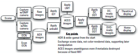
Figure 6.38 Color management using IIF. (Image courtesy of Joseph Goldstone.)

Input transforms process the image data code values produced by digital cameras and convert those data into Academy Color Encoding Specification (ACES) RGB relative exposure values. Color image data converted from various devices are brought together as ACES values, much as (roughly speaking) the ICC brings together data from various devices as PCS values.

The ICC architecture depends on metadata, in the form of ICC profiles. Transformed images identified as being encoded as per the ACES document are unambiguous without further metadata. Figure 6.39 maps the encoding given in the ACES document into the conceptual hierarchy of Figure 6.30.

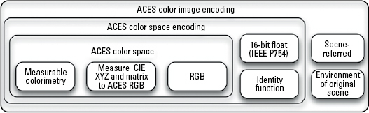
Figure 6.39 The ACES color image encoding. (Image courtesy of Joseph Goldstone.)

The color rendering performed on ACES data is always the same: a reference rendering transform (RRT) takes the ACES RGB relative exposure values representing the scene and transforms them into colorimetry suitable for display in a darkened theater by some idealized display device. The output of the RRT is then mapped through a device-specific output device transform (ODT) designed to approximate best the appearance of the ideal darkened theater image on some particular class of display and in some viewing environment, whether a digital projector, a desktop HDR display, or a Rec. 709 broadcast monitor.

Commercial Color Management Packages

As of early 2010, there were two commercial color management systems with substantial market penetration in the DMP industry: the Truelight system from FilmLight Limited and the cine-Space system from Cine-tal (originally developed by Rising Sun Research). Both are well engineered, widely used, and provide comprehensive documentation to supplement the information in this section,²⁵ both in the particulars of those systems and on color management for motion picture work. Neither uses the ICC or the IIF in their architecture or implementation.

Intersection with On-Set Practices

As discussed at the beginning of this section, the advantage of acquiring DMP image data in raw mode is that creative decisions are not irrevocably baked into the encoded image data. The disadvantage is that capture-time review of raw data requires some form of on-set color rendering for display. This is typically done by special-purpose hardware that interprets the video stream, applies color rendering for a high-quality on-set display, saves the transform, and passes that transform on as metadata to postproduction.

The color rendering is normally accomplished by a 3D lookup table (LUT) built by a manufacturer, by a digital imaging technician (DIT)—possibly at a rental company—or by a DP The look of this transform may be portably encoded in the color decision list (CDL) whose format is defined by the American Society of Cinematographers (ASC); some parts are not yet standardized and call for careful documentation and cooperative testing between the production and post-production facilities. Without such cooperation and in the absence of a full standard for the description of the desired look, a raw workflow may produce images that may be firmly locked to scene radiometry but which are aesthetically adrift, disassociated from the DP’s intent.

Some Desktop Color Management Caveats

Ideally (from a color engineer’s viewpoint, not a producer’s viewpoint) every artist would have his or her own screening room, and the issues about to be listed would not apply. Given that color-critical judgments will inevitably be made at the desktop, however, visual effects staff should be aware²⁶ of the following five factors that influence the artist’s perception of a displayed color, and two factors that influence the displayed color itself:

•   Glare from incidental light sources (a skylight, a neighboring cubicle’s desk lamp, etc.) reflecting off a display’s surface will lower color contrast and saturation. If the unwanted light is chromatic, the color’s hue will also be affected.

•   Viewing-angle dependencies (especially with LCD displays) can cause observers clustered near a monitor to each see a different color. The classic publicity shot of the heads of an artist and VFX Supervisor bent over a monitor virtually guarantees they are seeing different colors on the display surface.

•   A display’s correlated color temperature (CCT) is not an accurate predictor of its neutral chromaticity.²⁷ Use hardware and software that can calibrate a monitor’s neutrals to match a particular pair of CIE x, y chromaticity coordinates, since many perceived colors can share the same CCT.

•   Inappropriate color cues, such as a to-do note on a monitor bezel or even a white memo taped to a nearby wall,²⁸ will cause observers to misjudge the chromaticity corresponding to neutral colors. Movie audiences “white balance” to the content based on their memory of objects they “know” are white: snow, a white coffee cup, and the white letters on a road sign. Artists should adapt to neutrals in the subject material, as theatergoers do.

•   A light surround inflates perceived image luminance contrast. If a shot’s colors are chosen or adjusted with the image surrounded by a lighter background, that image might look low contrast in theatrical presentation. Craft-store black velvet or even stage duvetyne are better approximations to theatrical projection than a light aluminum bezel.

•   The absolute luminance levels of colors affect the perception of their colorfulness. If a desktop monitor’s peak white luminance (measured with a colorimeter or even a spot meter) is several times that of the luminance of projected white in a theater, the projected image will appear less vivid than its preview at the desktop.²⁹

•   The angular subtense of a color stimulus influences its appearance, as most people have learned when repainting their kitchen with colors chosen from small paint chips in a store rack. In the theater, always make color judgments from the same seat, and try to emulate this in the cubicle.

Two other things should also be kept in mind:

•   Monitor color reproduction gamuts merely approximate digital and film projection reproduction gamuts. Use desktop image review software that can flag regions where the color on the desktop display is known to be an inaccurate preview of the color of the final projected image.

•   That said, remember that a desktop display’s inability to preview a color that a digital projector might produce (or a film projector might project) is not a liability as long as none of the production’s content uses that color. The colors of a documentary on strip-mining for coal will probably not suffer if a desktop display cannot match the deepest indigo or most brilliant red of digital projection.

Bringing Color Management to Film Workflows

Today there are many more film theaters than there are digital theaters, and film projection will have a long tail-out. The dyes present in processed film register scene colors by modulating the way in which the film transmits light of various wavelengths. Any data metric for film-captured images, then, must have as its foundation some wavelength-dependent function; in the parlance of color science and international standards work, these wavelength-dependent functions are known as the spectral condition defining density.

Spectral Conditions Underlying Densitometric Data Metrics

For the motion picture industry, five spectral conditions are relevant. Two of them are used for process control: ISO Status M density’s underlying spectral condition helps in keeping negative development steady (or can be used forensically when development goes awry) and ISO Status A density’s underlying spectral condition serves the same function for print development. When a production assistant calls out lab variances at dailies, he or she is basing that assessment on Status A density. Process control densities are less than optimal for predicting projected color. For that purpose, three spectral conditions are used to determine printing densities, which numerically encode the way the print will register the colors encoded on the negative:

1.  Cineon printing density’s (CPD’s) spectral condition,

2.  the spectral condition of SMPTE RP-180,³⁰ and

3.  Academy printing density’s (APD’s) spectral condition.

Graphs of two of the three spectral conditions are shown superimposed in Figure 6.40, with the older RP-180 spectral condition indicated in thin lines and the newer APD in thick lines.

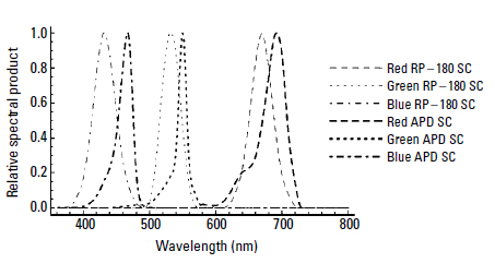
Figure 6.40 Spectral conditions defining density. (Image courtesy of Joseph Goldstone.)

The spectral condition for Kodak’s original Cineon printing density (circa 1993) was proprietary and never made public; the consequence was considerable scanner vendor-to-scanner vendor and facility-to-facility inconsistency in producing “Cineon” scans of the same negative; scanner vendors reverse-engineered the Cineon spectral condition independently.

Densitometric Color Spaces and Data Metrics

Not only are CPD and the printing density associated with SMPTE RP-180 showing their age in terms of applicability to contemporary print stock, but also the ranges of their associated color space encodings are now unable to cope with the extended density range registered on contemporary original camera negative (OCN) stocks such as Kodak 5219. Cineon and DPX both encode printing density into three 10-bit fields with the minimal pixel-value change indicating a 0.002 increment of printing density over average OCN base density. Cineon encoded the OCN average base density at code value 95, to avoid clipping pixels whose individual densities scanned at below the OCN average base density. When code value provision for this headroom is included, the larger contemporary OCN density ranges shown in Figure 6.41 cannot be encoded in a 10-bit field with single-bit changes indicating a 0.002 printing density increment.

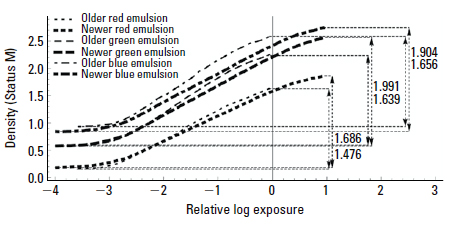
Figure 6.41 Encoding ranges and contemporary OCN densities. (Image courtesy of Joseph Goldstone.)

Users of Cineon or DPX color image encodings whose image content uses the full range of newer emulsions must either clip highlight values or use a nonstandard and nonportable printing density increment to squeeze the densities into the storage layout of the encoding. Although there appears to have been provision to indicate a nonstandard density increment in Cineon or DPX headers, no Cineon or DPX I/O libraries known at the time of this writing pay attention to the relevant header fields, and therefore production must carefully make each internal and farmed-out user of the image aware of the nonstandard encoding.

Academy Density Exchange Encoding (ADX) in its recommended ADX₁₆ form will provide 16-bit rather than 10-bit fields, supporting a density range of nearly 8.192 over base,³¹ and thus avoid this problem entirely. ADX-compliant scanners were estimated to become commercially available as soon as mid-2010.

Characteristics of Film Scanners as Image Capture Devices

Whereas the relationship between scene colorimetry and digital camera sensor linear output values can be reasonably approximated by a 3 × 3 matrix transform (much as is the case with additive displays), the relationship between scene colorimetry and scanner transmission sensor output values is much more complicated. The sensitivity of the multiple layers of film is complicated by crosstalk that can vary with the intensity of the exposing light, and by films that are designed to deviate from literal capture of scene colorimetry in favor of more pleasing colorimetry (exaggerating the green of grass, for example, or the blue of captured sky). Moreover, any crosstalk in film sensitivities is compounded by possible crosstalk at the scanner sensor level.

Film Unbuilding and Film Building

Analytic models of the relationship between scene color and captured density are considerably more complex than their digital counterparts. Most such models are proprietary, although Kodak and FujiFilm have cooperated with the AMPAS IIF effort in creating a transformation from APD densitometry to ACES colorimetry (that is, ACES RGB relative exposure values). In the IIF architecture, using this transform is termed unbuilding³² the film; inverting the transform (building the film) produces APD values from ACES RGB relative exposure values.

The Film Reproduction Gamut

Film’s continued use as a delivery medium is not just habit, nor is it purely a matter of the cost of converting theaters for digital projection. For those who originate their project on film, or who digitally capture or synthesize images using an encoding that supports a wide gamut, film provides certain colors that are not produced by any current commercially available digital projection system. Glacier ice, for example, contains a wealth of dark cyan detail that typically is clipped by digital projection, and certain deep pure yellows can be produced with film but not with current digital projection technology. That said, no film print can ever hit the deep red of a freshly painted fire engine, but digital projection systems can easily achieve the needed luminance and chromaticities.

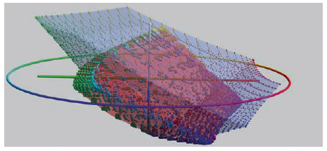
Figure 6.42 This color plate shows the relationship between the reproduction gamut of commercial-grade digital projection (sharp-edged color solid) and that of projected film (rounded edges). (Image courtesy of Joseph Goldstone.)

Film at the Desktop

The difficulty of modeling the nonlinear relationship between densitometrically encoded image data (that is, printing density values) and reproduced colorimetry is such that the traditional video card’s three independent 1D LUTs cannot provide the processing required for a credible prediction of projected film. Instead, 3D LUTs can be created to express the interdependencies between the color channels, usually by spectral measurement of filmed-out color cubes, each frame of the film-out being a full-frame patch of color. The resultant transmission spectra are combined with a spectral measurement of a film projector’s open-gate light bounced off a theater screen to predict the projected colorimetry of a film-out. Such characterization is available from most providers of color management software or through independent consultants.

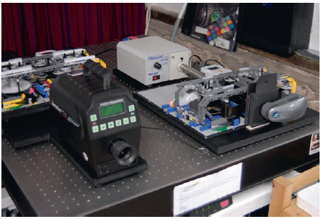
Figure 6.43 Spectral transmission measurement of a filmed-out color cube. (Note film loaded into right-hand unit.) (Image courtesy of Joseph Goldstone.)

DIGITAL INTERMEDIATE

Christopher Townsend

The digital intermediary is a part of the post process that is gathering more importance and relevance within the filmmaker’s toolbox. This phase of post-production is also known as color grading, timing, finishing, or more commonly, the DI. It has become a stage that can alter the entire look of a project. By enhancing, among other things, the color, saturation, and contrast palette, filmmakers can add drama and nuance, hence changing the mood of a piece. Knowing that most films go through a DI stage adds one more layer about which visual effects professionals need to be aware. Now, the image that leaves the visual effects facility and is “finaled” by the director is not necessarily the same image that appears in the final film in the theater. The line between what was traditionally done by a visual effects company and what can be done at the DI stage is getting more blurred all the time.

The DI stage can be an incredibly powerful finishing tool, allowing filmmakers to tweak a shot, often separating the image into different areas or layers, using power windows, rotoscoping, or mattes provided by a visual effects company.

Power windows are traditionally simple geometric shapes that are used as mattes or stencils, through which an image is enhanced in certain areas. For example, a circular power window may be used to brighten just the area of an actor’s face, or a rectangular one can be used to darken a sky.

Rotoscoping is basically a more complex (and more accurate and more versatile) version of power windows. The operator creates a spline around the area that needs to be enhanced, key-framing it if necessary.

Mattes from a visual effects company, for certain areas or objects, may be requested by the DI team to be used to protect or adjust specific areas of the shot. Creating mattes can add expense and additional workload for a visual effects company but can be very useful. The fear that all of those meticulously constructed composites can quickly be torn apart if mattes are not used judiciously is well founded, so such work should be carefully supervised.

What does this mean to the visual effects community? It means that images need to be protected; that is, they should have as much dynamic range as possible so that they can be pushed and pulled around without breaking. Sometimes a director, colorist, or cinematographer goes into a DI suite early in the process and creatively pregrades a sequence. If so, that information can be used while creating the visual effects. Depending on how different the intended look is from the original source photography, various approaches may be applicable.

Film is an analog process, with each piece of negative reacting slightly differently to light, to the chemical processing baths, to the scanning process, etc. As a consequence, there will always be undesirable discrepancies between shots, whether they be exposure or color related. As more and more productions are shot on HD, some of these variables are removed. Technically pregrading the plates, matching shot to shot, so that the same CG lighting rigs and basic composite color calls can be used, is often a good idea. Note that this sort of pregrade isn’t a creative one; it’s sometimes known as normalizing or neutralizing and is merely a unifying pass, rather than one that indicates the final look. This pregrade could be done as the shots are scanned or by a visual effects company. Generally, if the visual effects work seamlessly in the pregraded plates, with matching black levels, etc., then whatever is done to the final image should take everything in the same direction.

However, subtle nuances in the visual effects may be lost if the image is taken too far away from the original working color space. If the DI team, based on a creative pregrading session, knows exactly where it will take the final images, then working directly on these new color-corrected plates may be a good idea. Again, these color-corrected plates may be provided by the DI suite or scanning facility or created by a visual effects company, based on specified reference timing or match clips. These clips, which are individual frames, represent the intent for the entire sequence. In this case, a visual effects company would deliver its work integrated into plates with the final look.

A display LUT can be created to emulate the final desired look. This doesn’t affect the actual data within the image, but is an adjustment layer that is applied and shows what the final color correction will look like. Working on the original plates (or neutralized pregraded plates) may offer the best and most protected workflow. Artists and clients should both review the shots using the display LUT. However, the artists should also check that their work still looks integrated in the non-LUT version, because this is what will be delivered back to the DI suite.

If an extreme color correction is going to be desired, a more complex approach is often necessary: a combination of all of the above. First, the colorist technically pregrades the plates to neutralize them shot to shot. Then, based on the intended final look, the colorist creatively grades the plates. Depending on how far away that is from the original photography, a percentage of that look (maybe 10, 20, or 50%) should be used to color correct the shots, which now become the plates with which the visual effects company will work, and the color space in which the completed shots are sent to the DI. However, a supplementary LUT needs to be created to emulate the final look and should be used by artists and clients to review the shots. Again, the artists should also check that their work still looks integrated in the non-LUT version.

So, how does one choose the best approach? As is often the case in visual effects, there is not necessarily a correct answer. If the final look is not far off from the original photography, then working directly on the technically pregraded plates is the best solution. If the director and his team know exactly where they want the images to end up, then working on creatively pregraded plates makes sense. If there is any doubt that the final look is undetermined, then a combination is preferred.

As stereographic filmmaking becomes more popular, it is worth noting the differences and complexities that this adds. Often left and right images have different colors and exposures, so this needs to be addressed. Frequently, there are geometric differences between the eyes, and again, using scaling and image warping tools, these can be corrected in the DI. In stereo, a matte has to be offset for each individual eye. However, its shape also needs to be adjusted, because the shape of the object will be different, due to perspective shifts between one eye and the other.

Many DI suites offer toolsets that are the equal of some basic compositing systems. This means simple compositing (keying, tracking, stabilizing, keyframe animating, and layering as well as the expected color controls) can be done within the suite. Huge advantages are realized by working on the final shots in a known calibrated environment on a large screen. Having the director (and other members of the creative team) work directly with the artist (usually the colorist in this case) removes any feedback loops and potentially saves a huge amount of time. The problem, however, is that it usually costs a huge amount of money to use time in the DI suite, so this is often not a good use of resources, but it illustrates the potential power of such a tool. Whatever approach is chosen, discussing it with the key members of the DI team early in the process is vital; confirming the specific technical requirements and testing that pipeline to check the results are also highly recommended. After all, the digital intermediary is something that should be embraced as an integral part of the visual effects pipeline.

VFX EDITORIAL

Greg Hyman, David Tanaka

This section is not intended to be an absolute description of a VFX Editor’s job. Each visual effects movie represents its own set of challenges and each studio, or visual effects facility, has its own unique pipeline. The purpose of this section is to give a brief history and overview of the many standard responsibilities and procedures a VFX Editor typically faces on a modern visual effects movie.

This section describes the responsibilities and procedures inherent to visual effects editing. It also provides key background information on how the role has evolved through the years, as well as a better understanding of how editorial information is organized and disseminated clearly and accurately in the modern age.

Much of what VFX Editors do is process oriented and deals with numbers—numbers such as shot lengths, handle lengths,³³ cut lengths, key numbers,³⁴ timecode,³⁵ scene numbers, take numbers, lab roll numbers, and on and on. Then they translate those numbers into other numbers so that producers, VFX Supervisors, scanners, animators, lighting technical directors, and compositors can understand and work with them. Finally, they disseminate these numbers to companies hired to create the visual effects: scanning, visual effects, post-production, and digital intermediate facilities. And when the numbers change (and they will often), VFX Editors start the process all over again.

On large shows multiple VFX Editors may be tracking this information: one in the cutting room and one in each of the visual effects facilities, for example. Regardless of where VFX Editors work, their jobs are basically the same: They track and exchange the same set of numbers. The numbers they track are vital to the creation of visual effects shots because they define what elements are to be used in a shot, the order in which these elements are to be composited, how long the shot is, and how the shot has changed over time. They also give VFX Producers the information necessary to budget the creation of the shot(s). If these editorial numbers are wrong or incorrectly interpreted, they can cost the visual effects facility and the production valuable time and money.

Given the complexity of the job, the VFX Editor is often one of the longest serving crew members on a movie.