1.1 Scales, symbols and equations

When beginning to learn electronics, many of the terms used will be new to you. Just like mathematics and physics, electronics has its own language and so this chapter begins by discussing some of the fundamental elements involved. Before we do this, it is important to know a little about the mathematical scales used and how they relate to each other – they can often be a major source of confusion when learning some of the concepts and equations used in later chapters. Table 1.1 lists the common mathematical powers of ten and the symbols used to represent them.

The table shows how large and small quantities can be scaled to make them easier to work with – it is much easier to refer to a 3MΩ resistor than a 3,000,000Ω resistor when listing components for a circuit. The key to working with powers of ten is to carry out the following steps:

Often the most confusing thing about powers of ten is when a scaling prefix is applied to a number that is already scaled – you may sometimes encounter a capacitance value like 0.22μF which is equivalent to 220nF (0.000000022F)! Another downside of scaling in this way occurs when performing calculations with the actual quantities involved – particularly smaller values like μ, n and p. Let’s say we are working with two voltages that have values of 10mV and 8μV (we’ll learn about voltage later in the chapter), and that we want to add them together. The following example illustrates where problems can occur due to scaling if each step of the calculation is not performed correctly.

1.1.1 Worked example – adding voltages

We will learn more about adding voltages in chapter 3, but for now let’s look at how scaling affects the mathematical process involved.

Q1: What is the total voltage V_tot, as a result of adding 10mV and 8μV?

Answer: The total voltage V_tot is approximately 0.01V (rounded to 2 decimal places).

The example above seems simple enough, but what if the wrong scaling factor was used for either the 10mV or the 8μV values – the result would be very different! This can be a problem when learning electronics, where the quantities used are often related by completely different orders of magnitude. The reason for this is partly due to the evolution of knowledge over a long period of time, where the definition of a quantity and its scale were made prior to their current usage – for example, an audio signal capacitor will often be in the n or ρ range, whilst the resistors we will use will mainly be in the kΩ range. We will see another example of this later in the chapter when we encounter conventional current flow – it is conventional because of its historical precedent, even though electrical charge actually moves in the opposite direction! Although you may have learned other ways of doing arithmetic with powers of ten, in this book we will always write out the full quantity to avoid arithmetic errors – it may seem a little pedantic, but you can always double check the full value by counting the number of decimal places involved.

Another difficult aspect of electronics can be the symbols used for scales and quantities involved – you have already seen scaling symbols like k, c, m, μ, n, ρ in the table above, but symbols like ohms (Ω), watts (W), amperes (A), volts (V) and farads (F) were also used to define some of the different quantities used during the book. There is no easy way to learn symbols other than by practice, and as with scaling factors it is important to remember that learning a new set of concepts takes time – learning the language that represents them is a separate (though related) task that will also take a similar amount of time and effort. We will encounter this problem again when we learn how to program the Arduino in chapters 4 and 5 – programming concepts are what an Arduino can do, the syntax of the C language is how you tell the Arduino to do it! In all instances, if you take your time to follow all the steps in each task you will begin to see the method behind them.

In comparison to scales and symbols, the electronics equations we will use are relatively straightforward and do not employ complex mathematical operations like those found in other audio areas such as acoustics or digital signal processing. The main problem with learning electronics equations is that the scales and symbols involved introduce a new layer of complexity to adding, subtracting and multiplying quantities. For example, one of the most widely used equations in electronics is Ohm’s Law:

Voltage, V = IR(1.1)

	V is the potential difference in volts (V)
	I is the current in amperes (A)
	R is the resistance in ohms (Ω)

The equation above is arranged to allow you to learn the relationship first, then consider the quantities involved afterwards – this convention is used for all equations in this book. We will learn more about Ohm’s Law in chapter 3, but for now consider the mathematical operation involved, where one quantity (voltage) is equal to another two quantities multiplied together. This is not a difficult mathematical relationship to grasp, but when you combine it with scales, symbols and other circuit analysis methods that we will learn (like Kirchoff’s Laws) it can often feel like it has become quite complicated. Thus, before you learn how to analyse a circuit, try to remember that you already know the mathematics involved – it’s the other elements that are new and sometimes confusing to learn!

An important thing to note about electronics equations is that many of them deal with proportions that are based on fractions. In the modern digital world computers are used for speed and accuracy, but when circuit theory was first proposed this means of calculation did not yet exist. Thus, when working with series and parallel circuits in chapter 3 you will learn about adding and multiplying fractions and also about reciprocals – 1 divided by the quantity. This will perhaps be unfamiliar to you (even if you studied it at school) as fractions are not used very much in modern computation – the fraction is usually converted to a percentage or simply to a decimal number, which in itself can create a significant level of scaling to quantify the value accurately (e.g. the fraction 13 can only be approximated using decimal numbers). The important point about fractions in electronics is that they are often used to represent ratios between quantities, as in the next example:

1.2 Electrical fundamentals

When learning electronics, you will come across terms like current, voltage and resistance as part of the language used to describe the behaviour of circuits. The basis of all these fundamental concepts is electrical charge, which defines how subatomic particles are either attracted to or repelled by one another based on their positive or negative polarity. Electrically charged particles follow simple rules:

We are interested in electromagnetic force, which defines how particles actually move based on their charge. Although a particle can be electrically charged, it requires an electromagnetic force to move it closer to an opposite charge (or further away from a like particle). This is fundamentally important when learning about charge – the force needed to move a charge is not the charge itself. In a simple model of the atom, nucleons can either be a proton with a positive electrical charge, or a neutron that has no charge. An atomic nucleus is formed by a certain number of protons and neutrons that are bound to each other by the strong nuclear force (Figure 1.1).

The strong nuclear force is greater than the electromagnetic force at very short distances, and so it helps bind neutrons to protons to prevent the positively charged protons from repelling each other – this creates an atomic nucleus. It can help to think of neutrons as subatomic ‘spacers’ that hold positive protons together, without them the electromagnetic force created between these like particles would split them apart. Apart from nucleons, the other major component of atoms are electrons, much smaller negatively charged particles that orbit the nucleus within different shells (Figure 1.2).

The diagram shows each electron shell as having a principal quantum number (n), which defines the maximum number of electrons that can orbit within that specific shell using the relation 2n². Although we don’t need to completely derive this proof for our electronics work, it is important to note that the factor of 2 in this relationship occurs because the electrons in each shell orbit in pairs (we will return to this in chapter 2 when we look at electromagnetic induction). If the maximum number of electrons are not present within a given shell, then there are holes available for other electrons to move into. Electrons have more energy than holes, so when an electron fills a hole the difference in energy is released as a photon – the fundamental particle of all electromagnetic radiation (this includes light – you may already have heard about photons in this way). In an atom, the nearest shell to the nucleus has the strongest electromagnetic force between positively charged protons and negatively charged electrons. This means that the closest electron shells have the strongest attraction to protons in the nucleus. On the other hand, the outer shell contains valence electrons – free electrons that can be attracted to other positive charges outside the atom because they are not held by as strong an electromagnetic force (Figure 1.3).

In Figure 1.3, valence electrons are not strongly bound to the positive nucleus of their own atom and so they can be attracted to another nucleus – but only if this nucleus has holes available in its own valence shell. If an atom has a full valence shell it is considered to be more stable (in chemistry they are defined as less reactive), but those with holes have the potential to accept new electrons. We define net electrical charge as the difference between the number of protons and electrons in an atom (net being the result of a sum or difference), where electrically charged atoms are known as ions:

The difference in net charge is measured in coulombs (C), which is a Standard Unit (SI) for the measurement of electrical charge. A coulomb is defined as a net difference of 6.24 quintillion electrons ( 6.24×1018) for a negatively charged anion (or the same net difference in protons for a cation). If an electron leaves an atom, the net electrical charge for that atom becomes more positive. On the other hand, if an electron passes into the orbit of a new nucleus then the increased number of electrons means that the net electrical charge for that atom becomes more negative (Figure 1.4).

In the diagram, the most important thing to notice are the holes in the positive cation charge: these are spaces that valence electrons can move into. This is a very important point to remember, as the concept of a positive charge can initially be confusing – a positive charge has holes for electrons to move into. Electrons are the only particle that can move from one nucleus to another (under normal conditions), so this effectively means that electrical charge is passed from atom to atom by the movement of electrons. This idea of charge flowing can be confusing at first, as we are actually talking about the movement of electrons changing the net charge of each atom they pass through – the change in net charge moves with them. A useful analogy for this is a Newton’s Cradle, where the inner spheres effectively do not move, but the force of the initial collision is transferred through them to reach the outer sphere (Figure 1.5).

Now we have a basic understanding of electrical charge and how it moves, we can define one of the fundamental units of electronic circuits:

One ampere of current is equivalent to one coulomb of charge flowing for one second of time. Time is the important difference between charge and current, as it is used to define the rate at which charge flows – 1 coulomb of charge flowing every 2 seconds would be 0.5A of current. You may already have encountered amperes (often called amps) as a common means of rating electrical and electronic equipment (Table 1.2).

Current ratings are very important, as supplying the wrong level of electricity to a device can easily damage or destroy it. Similarly, a high-current device will require a connection that can provide that current – thus a mobile device charger will not be able to power a kettle, but a 13A kettle plug will deliver enough current to destroy a mobile phone battery. The size of an electrical current is effectively the amount of electrons moving past a given point, and the increased energy created by more electrons moving generates heat that requires thicker cables and more insulation to protect those handling them (Figure 1.6):

Conductivity defines the ability of a material to allow electrical charge to pass through it, where metals like copper have a high level of conductivity because they have less stable valence shells than other materials. This means copper wire is commonly used to conduct electricity, and thicker copper wires are able to move more electrons without overheating. We will learn more about resistivity (which is the opposite of conductivity) in the next section, but for now the next important concept to define is that of potential difference. You may already be familiar with the term voltage, but this is actually the unit of measurement for the potential difference between two points in an electronic circuit. We will use potential difference extensively in our audio circuit calculations, but it is often misunderstood as a concept and hence can cause confusion when learning the basics of electronic circuit theory. Potential difference is a term analogous with other areas of physics, and so we can use other forces to explain it more easily. For example, you may have learned that the potential energy of an object at a certain height is greater than that of one at a lower level – in this case the effect of gravity means that the higher object has more potential to move within the gravitational field by falling to the ground (Figure 1.7).

The Earth’s gravity is a force that pulls objects towards it, and the further away an object is from the surface of the Earth the more gravitational energy needed to pull it back. An object at a certain height above the Earth is defined as having potential energy because there is no actual force being applied to the object yet – only the potential for that force to be applied if the object was free to move. Taking the diagram in Figure 1.7 as an example, if you hold a ball (sphere) in your hand you are providing the kinetic energy needed to cancel out the potential energy of the ball to fall to Earth. If you let go of the ball, the potential energy of the ball is now converted into kinetic energy by the force of gravity acting upon it – the ball falls to the ground. We measure potential energy in the Standard Unit (SI) of joules (J) as the product of mass, gravity and height (from the surface of the Earth) using the equation:

	P is the potential energy in joules (J)
	m is mass of the object in kilograms (kg)
	g is acceleration due to the gravity of Earth in metres per second (m/s2) – this value is defined as a constant of 9.8 ms2
	h is the height of the object in metres (m)

To understand this relationship, it can help to remember that the original kinetic energy needed to lift the ball into the air in the first place is effectively the same as the kinetic energy that would be created by the gravitational force if you let the ball go (this is known as conservation of momentum). This kinetic energy is known as the work done to move an object between two points:

	W is the work done in joules (J)
	f is the force needed to move the object in newtons (N)
	d is distance the object moves in metres (m)

Work done helps us distinguish between potential energy and kinetic energy – the force defined in the above equation can be seen as the kinetic energy needed to move the ball over a certain distance, rather than the potential for work done that exists prior to us letting the ball go. We can now apply the same idea to electrically charged ions to define electrical potential, where a positively charged cation will attract electrons from a negatively charged anion towards it (Figure 1.8).

In the diagram, the positively charged cation on the right has holes that can accept valence electrons from the negatively charged anion on the left. This means that the positive cation has the potential to move charge by attracting electrons towards it. The directional lines represent the resulting electric field that is created by the potential difference between the two charges, showing where there is potential for the movement of electrons (to restrict the size of the diagram, many of the wider field lines have been truncated). These lines are much like those shown in Figure 1.7, which indicate the direction of force exerted on the mass of an object by the gravitational pull of the Earth. As a result, we consider the positive charge to have a higher potential than the negative, which allows us to define the potential difference between the two charges as the work done in moving electrons between them:

	V is the potential difference between the two charges, in volts (V)
	W is the work done in moving electrons between charges, in joules (J)
	C is the number of electrons being moved, in coulombs (C)

The equation above is similar to our previous example in Figure 1.7 of potential energy – in the same way that gravity must do work to move an object that has potential energy closer to Earth, so the work done in moving a certain amount of charge is equivalent to the potential for that charge to move. The actual potential difference is governed both by the charge being moved (in coulombs) and the work done (in joules) to move it. This allows us to define our second fundamental concept of potential difference:

We measure potential difference (in volts) as the work done (in joules) needed to move a charge (in coulombs) between two points – 1 volt equates to 1 joule of work to move 1 coulomb of charge. The main problem you will encounter is that potential difference is commonly referred to as voltage – when actually what is meant is a potential difference measured in volts! To keep things simple, voltage will be used as it is the most common term you will encounter in electronics. Having said this, it can often be difficult for new learners when multiple terms are used interchangeably. We will be using voltage extensively in this book, so spend a little time reading this section again until you are comfortable with the concept of the potential to move charge.

As you now know, voltage is the potential for an electrical charge to move – not the work done by electrons when they are moving as an electrical current. The simplest practical example of potential difference is a battery, where chemical reactions between different elements are used to produce ions (Figure 1.9).

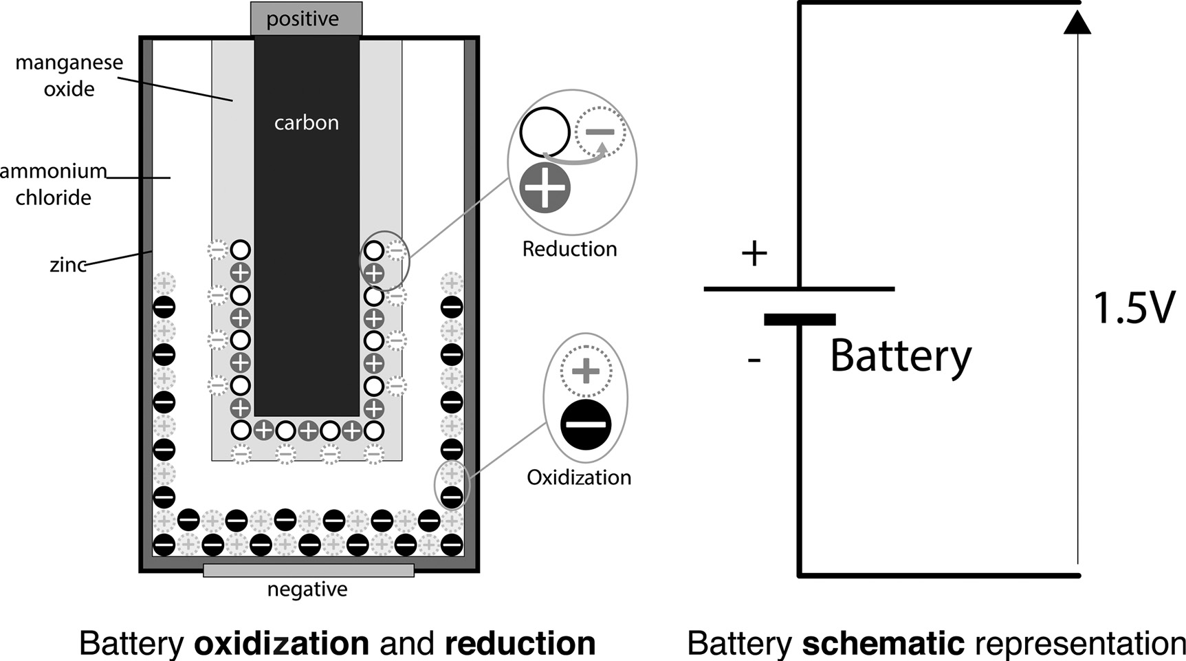
In the above example, zinc atoms oxidize (dissolve) in ammonium chloride leaving spare electrons behind, which creates an overall negative net charge of anions that collect at the metal base plate. At the same time, the manganese oxide and ammonium chloride reduce (removing electrons by using them to produce hydrogen) to leave holes and thus create an overall positive net charge of cations that collect around the carbon conductor (chosen because carbon does not oxidize like metals).

We now have a negative and positive terminal, and just as we saw in Figure 1.8 the imbalance between the charges at each terminal creates a potential difference between them. The right-hand diagram shows a schematic representation of the battery, where the arrow going from negative to positive indicates the potential difference between battery terminals. We refer to linked combinations of electronic components as circuits because they provide a circular path for current to flow. The schematic of the battery shown above is known as an open circuit – there is no path for a current to flow. If we were now to connect a single wire between the anode and cathode terminals of our battery, we would create what is known as a short circuit (Figure 1.10).

As current can now flow through the circuit from anode to cathode, the battery terminals will start to overheat due to the free movement of electrons. This can cause damage to the battery, other components or even the user of the circuit – thus we always avoid short circuits in practice! However, the biggest conceptual problem with the above diagram is the definition of conventional current flow on the right – how can this be conventional when electrons move in the opposite direction from negative to positive!

To this day, we still define circuits in terms of their positive potential difference and then analyse the flow of current going from positive to negative (or ground). You will find that every textbook (and university electronics programme) teaches in this way, so the same convention is used in this book to be consistent with the rest of the field. As our primary focus is to learn how to apply electronics theory to audio circuits, the direction of current flow is noted purely to disambiguate the concept for your own understanding. Though the flow of conventional current is effectively incorrect, in practice it makes no difference to the electronic calculations we will perform as long as we always calculate in a single direction. We will learn how to analyse basic circuits in the next chapter, and from now on we will use conventional current flow in all of our circuits. For now, let’s return to the problem of our battery overheating in Figure 1.10, as this short circuit demonstrates undesirable behaviour – a battery has a positive cathode and a negative anode, so when a current flows directly from one to the other it creates significant heat. As a result, we need to control the flow of current in all our circuits to prevent damage to components (or even the user). To do this, we define our third fundamental concept of resistance:

We learned in the previous section that less stable valence shells (i.e. those with more holes) make it possible for electrons to move and thus for electrical charge to flow. This is why materials like copper (and other metals) are good conductors – they have a relatively high number of holes when compared to insulators like glass (which is made from the more stable element of silicon). We use materials like copper to conduct the flow of charge (current) in a circuit, but we can also use them to create resistance within a circuit. To do this, we can combine some of what we learned in Figure 1.3 about current and the thickness of a wire with what we learned in Equation 1.3 about work done being related to the distance between points of electrical potential to understand how a wire wound resistor works (Figure 1.11).

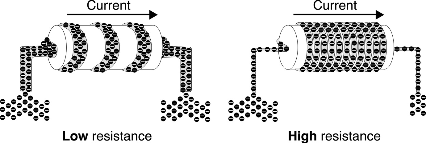
In this diagram, the copper coil in the left-hand example has thicker wire – it can carry more charge. This coil also has fewer turns, and so the current has a shorter distance to travel within the resistor (recall Equation 1.3 where Work done, W = f × d). This means it presents less resistance to the flow of current than the right-hand example, where a thinner wire with more turns will do more to resist the flow of charge – it will have a higher resistance value. There are many ways to create resistive components (e.g. carbon pile/film/printed) but wire wound resistors like those shown in the diagram above are particularly important because audio applications often use long cables for input (e.g. microphones) and/or output (e.g. loudspeaker) signals. Thus, understanding that all conductive materials have a resistance that varies with both length and thickness is of practical benefit when analysing the input and output requirements for amplifier circuits (we will learn more about this in chapter 2).

Among other fundamental contributions to electronics, George Ohm defined resistance as the relationship between the resistivity of the material used, the distance (length) the current must travel and the surface area (thickness) of the material involved:

Resistance,R=ρ×LA

	R is the resistance in ohms (Ω)
	ρ is the resistivity of the material used in ohm metres (Ω m)
	L is length of the material in metres (m)
	A is surface area of the material in square metres (m2)

Resistivity varies significantly between materials, with a conductor like copper having a value of around 1.72 × 10⁻⁸ Ω m (0.0000000172), whilst an insulator like glass has a resistivity of around 1 × 10¹⁴ Ω m (100000000000000). Resistance values are defined by colour-coded bands marked on the body of the resistor as shown in Figure 1.12

The first example in the diagram is a 4-band resistor, where the value is defined by the first two digits (colours of red and black – giving 20) multiplied by the scaling factor (orange for 1k) to give a resistance of 20kΩ. The second example is a 5-band resistor, which uses three digits (220) multiplied by the same scaling factor (1k) to give 220kΩ. These examples are of low tolerance (silver means a value of 10%) and in practice this can often mean a cheaper component – even though it is marked with silver or gold!

In the next chapter we will learn how resistance can be used by sensors to measure changes in real-world quantities, and in chapter 3 we will learn how to calculate the resistance needed for a real circuit. For now, we can revisit our battery short circuit from Figure 1.10 to see how we can include a resistor to prevent the battery from overheating (Figure 1.13).

In this circuit, the potential difference between the terminals of the battery is now ‘seen’ across the terminals of the resistor and so a short circuit across the battery is avoided – the potential for charge to move is now related to how much the resistor reduces the current flowing through it. It is important to remember that the resistor resists the flow of charge, and in chapter 3 we will learn how to use Ohm’s Law to calculate the required resistance needed when using power either from our Arduino board or from a separate battery.

In practice, if we connected a voltmeter across the terminals of the resistor to measure the actual voltage the connections between the resistor and battery will also present a (small) resistance to the flow of current (remember that all wires have resistance) and thus we will see a slightly lower voltage reading across the resistor than across the battery itself. This is particularly relevant in audio circuits, where we will often work with signal cables that are several metres long – even longer in live sound systems. These cables will have an increased resistance (and also a capacitance) due to their length, and in practice it is important that we bear this in mind when designing our audio systems to work with them. For now, we have a circuit where the flow of current is controlled by the resistor and we can use this as the basis of our first practical electronic circuit to light up a light-emitting diode (LED) (Figure 1.14).

In this circuit, the 150Ω resistor is used to limit the current flowing into the LED to prevent it from burning out. Without the resistor controlling the amount of current, the Arduino would supply too much current for the LED and it would burn out (creating a short circuit). Notice that LEDs have a specific polarity, where the longer leg is the positive terminal of the component. You may also notice that the words anode and cathode seem similar to anion and cation – this is another example of the confusion that can be caused by conventional current flow! We will learn more about how this circuit works in chapter 3, but for now the tutorial below will use it to introduce the Tinkercad application that we will use for some of our early circuits.

1.3 Tutorial – introduction to Tinkercad

Tutorials are used throughout this book to learn how to apply the concepts we have learned. All tutorials follow a series of steps that should allow you to successfully complete the task involved. It is vital that you do not skip any steps, as the tutorials in later chapters are designed to guide you through some of the common problems and mistakes that can occur when learning about audio electronic circuits. In this tutorial, we will do the following:

The first thing we need to learn is how to read a breadboard. A circuit breadboard is a very useful prototyping tool, where components can be added to a circuit by placing them into specific pins in the board. The underside of the board is a series of metal contacts that are connected in columns – except for the power lines on the outside, which are connected in rows (Figure 1.15).

It can initially be confusing to work with a breadboard, as the power lines create a visual cue that suggests all other pins are also connected on rows. It can help to think of a breadboard like a crossword puzzle, where power (is) across and signals (are) down. The breadboard is also split along the middle of each column (a–e, f–j) to create two separate columns on the board – in later projects we will see how this allows us to add a lot more components to a single board. The best way to learn breadboard layouts is by practising with them, but there are some initial guidelines you can follow. Whenever you are designing a breadboard circuit layout, the best approach is to start with the first positive component connection in the circuit and place it somewhere near a power row (leaving one pin free to connect to the power rail itself). Then, add each subsequent component by placing its positive terminal on the same column as the negative terminal of the previous component – they are now linked because every pin in each column is already connected (Figure 1.16).

Notice the resistor in this figure is connected on pins [i2–i6], which then allows a connection from the power line above to be added to pin j2 – because the resistor is also connected to column 2 it will now receive power. The final step is to add a ground connection to column 7, which will link the negative terminal (short leg) of the LED to ground (Figure 1.17).

It is not unusual for you to find this type of layout difficult (and a little frustrating) when you begin working with breadboard circuits – it can take time to remember the simple rule: power across and signals down. For the tutorial below, make sure you follow all steps in sequence to avoid getting mixed up by the breadboard layout; as time goes on it will become more familiar to you.

Tutorial steps

If you have followed all steps in the tutorial and have a lit LED in your simulation window, then well done – you have completed your first electronic circuit! We will use Tinkercad for other circuits in later chapters (particularly those that involve Arduino code), so it is important to learn how to use it as quickly as possible to avoid the tool becoming a stumbling block in your audio electronics learning.

At this point, we have now covered all three fundamental elements needed to begin learning about electronic circuits:

We will be using current, voltage and resistance throughout this book so it can be useful to refer back to this section if you find some later concepts difficult to grasp. At the fundamental level, everything in electronics is about the movement of electrical charge – we measure either this level of movement or the potential for it to move (most of our circuits will use voltage changes rather than current). Resistance is used to control the movement of electrical charge, and this is how all circuits operate – even more advanced components like capacitors and semiconductors are all resistive in some way, so these three elements will form the core of all your learning in audio electronics. The example project below will take you through the steps needed to build the tutorial circuit – one of the aims of this book is to have at least one practical project at the end of each chapter that covers what you have learned. In later projects we will focus more on audio circuits, but the example project aims to use the minimum amount of components to get you up and running with a practical circuit straight away.

1.4 Example project – getting started: an Arduino-powered LED light

The example project will use an Arduino with a 150Ω resistor, LED and breadboard to build the circuit we have just simulated in Tinkercad – which again highlights its usefulness as a prototyping tool for Arduino. To build this project, you will need the following components (Figure 1.17):

We will build our first circuit powered by the Arduino based on the schematic in Figure 1.19 (used in the previous tutorial):

In each project in the book, every build stage begins by showing the schematic for that stage and then its breadboard layout. In the opening chapters, we will also include the current flow for this layout to help you follow the breadboard layout process, and also as a check to ensure you have set everything out correctly (Figure 1.20).

Now we have a plan for our component layout, we can begin to build the circuit on breadboard.

Project steps

1.5 Conclusions

In this chapter, we have begun learning some of the fundamental methods and concepts of electronics. We found that scales, symbols and equations are effectively the language of electronics – all languages take time to learn. We also covered three fundamental concepts that we will use throughout this book: current, voltage and resistance. Voltage can be a difficult concept to understand, and we will return to it again in chapter 3 to reinforce what we have learned. The tutorial introduced the Autodesk Tinkercad online application for testing Arduino code and circuit designs – we will use this application again in the following chapters. The final project built a prototype of the tutorial circuit, a first practical circuit that lights an LED.

In the next chapter, we will learn the basic elements of an electronic system that combines inputs from sensors with outputs to actuators. This will help us understand the requirements of our audio circuits and what components we need to design them. When we learn how to program the Arduino controller in chapter 4 we will use our knowledge of systems to consider how it can be used to control the processes carried out by our circuits, so it is important to begin with a conceptual understanding of how this is implemented.

1.6 Self-study questions

In each chapter, a short set of questions are provided that aim to enhance your learning of the topic. Such questions can often be ignored because they are either considered by the learner to be too easy (or too difficult), or sometimes the learner is keen to progress onto more interesting topics and doesn’t want to be slowed down by what they believe to be yet more examples of the same things they have just learned. One of the reasons for self-study questions is to develop your practice of electronic theory, to make sure you build on a set of solid examples that will help you to reduce the mistakes you make when learning. As mentioned at the beginning of the chapter, learning can be significantly impeded by an increasing belief that ‘this is too difficult’ based on errors or mistakes in your work.