
Optimal Labor Income Taxation
Thomas Piketty* and Emmanuel Saez†,‡, *Paris School of Economics, Paris, France, †Department of Economics, University of California, 530 Evans Hall #3880, Berkeley, CA 94720, USA, ‡National Bureau of Economic Research, USA, *[email protected], ‡[email protected]
Abstract
This handbook chapter reviews recent developments in the theory of optimal labor income taxation. We emphasize connections between theory and empirical work that were initially lacking from optimal income tax theory. First, we provide historical and international background on labor income taxation and means-tested transfers. Second, we present the simple model of optimal linear taxation. Third, we consider optimal nonlinear income taxation with particular emphasis on the optimal top tax rate and the optimal profile of means-tested transfers. Fourth, we consider various extensions of the standard model including tax avoidance and income shifting, international migration, models with rent-seeking, relative income concerns, the treatment of couples and children, and non-cash transfers. Finally, we discuss limitations of the standard utilitarian approach and briefly review alternatives. In all cases, we use the simplest possible models and show how optimal tax formulas can be derived and expressed in terms of sufficient statistics that include social marginal welfare weights capturing society’s value for redistribution, behavioral elasticities capturing the efficiency costs of taxation, as well as parameters of the earnings distribution. We also emphasize connections between actual practice and the predictions from theory, and in particular the limitations of both theory and empirical work in settling the political debate on optimal labor income taxation and transfers.
Keywords
Optimal taxation; Behavioral responses to taxation; Means-tested transfers; Redistribution
1 Introduction
This handbook chapter considers optimal labor income taxation, that is, the fair and efficient distribution of the tax burden across individuals with different earnings. A large academic literature has developed models of optimal tax theory to cast light on this issue. Models in optimal tax theory typically posit that the tax system should maximize a social welfare function subject to a government budget constraint, taking into account how individuals respond to taxes and transfers. Social welfare is larger when resources are more equally distributed, but redistributive taxes and transfers can negatively affect incentives to work and earn income in the first place. This creates the classical trade-off between equity and efficiency which is at the core of the optimal labor income tax problem.
In this chapter, we present recent developments in the theory of optimal labor income taxation. We emphasize connections between theory and empirical work that were previously largely absent from the optimal income tax literature. Therefore, throughout the chapter, we focus less on formal modeling and rigorous derivations than was done in previous surveys on this topic (Atkinson & Stiglitz, 1980; Kaplow, 2008; Mirrlees (1976, 1986, chap. 24); Stiglitz, 1987, chap. 15; Tuomala, 1990) and we try to systematically connect the theory to both real policy debates and empirical work on behavioral responses to taxation.1 This chapter limits itself to the analysis of optimal labor income taxation and related means-tested transfers.2
First, we provide historical and international background on labor income taxation and transfers. In our view, knowing actual tax systems and understanding their history and the key policy debates driving their evolution is critical to guide theoretical modeling and successfully capture the first order aspects of the optimal tax problem. We also briefly review the history of the field of optimal labor income taxation to place our chapter in its academic context.
Second, we review the theoretical underpinnings of the standard optimal income tax approach, such as the social welfare function, the fallacy of the second welfare theorem, and hence the necessity of tackling the equity-efficiency trade off. We also present the key parameters capturing labor supply responses as they determine the efficiency costs of taxation and hence play a crucial role in optimal tax formulas.
Third, we present the simple model of optimal linear taxation. Considering linear labor income taxation simplifies considerably the exposition but still captures the key equity-efficiency trade-off. The derivation and the formula for the optimal linear tax rate are also closely related to the more complex nonlinear case, showing the tight connection between the two problems. The linear tax model also allows us to consider extensions such as tax avoidance and income shifting, random earnings, and median voter tax equilibria in a simpler way.
Fourth, we consider optimal nonlinear income taxation with particular emphasis on the optimal top tax rate and the optimal profile of means-tested transfers at the bottom. We consider several extensions including extensive labor supply responses, international migration, or rent-seeking models where pay differs from productivity.
Fifth, we consider additional deeper extensions of the standard model including tagging (i.e., conditioning taxes and transfers on characteristics correlated with ability to earn), the use of differential commodity taxation to supplement the income tax, the use of in-kind transfers (instead of cash transfers), the treatment of couples and children in tax and transfer systems, or models with relative income concerns. Many of those extensions cannot be satisfactorily treated within the standard utilitarian social welfare approach. Hence, in a number of cases, we present the issues only heuristically and leave formal full-fledged modeling to future research.
Sixth and finally, we come back to the limitations of the standard utilitarian approach that have appeared throughout the chapter. We briefly review the most promising alternatives. While many recent contributions use general Pareto weights to avoid the strong assumptions of the standard utilitarian approach, the Pareto weight approach is too general to deliver practical policy prescriptions in most cases. Hence, it is important to make progress both on normative theories of justice stating how social welfare weights should be set and on positive analysis of how individual views and beliefs about redistribution are formed.
Methodologically, a central goal of optimal tax analysis should be to cast light on actual tax policy issues and help design better tax systems. Theory and technical derivations are very valuable to rigorously model the problem at hand. A key aim of this chapter is to show how to make such theoretical findings applicable. As argued in Diamond and Saez (2011), theoretical results in optimal tax analysis are most useful for policy recommendations when three conditions are met. (1) Results should be based on economic mechanisms that are empirically relevant and first order to the problem at hand. (2) Results should be reasonably robust to modeling assumptions and in particular to the presence of heterogeneity in individual preferences. (3) The tax policy prescription needs to be implementable—that is, the tax policy needs to be relatively easy to explain and discuss publicly, and not too complex to administer relative to actual practice.3 Those conditions lead us to adopt two methodological choices.
First, we use the “sufficient statistics” approach whereby optimal tax formulas are derived and expressed in terms of estimable statistics including social marginal welfare weights capturing society’s value for redistribution and labor supply elasticities capturing the efficiency costs of taxation (see Chetty, 2009a for a recent survey of the “sufficient statistics” approach in public economics). This approach allows us to understand the key economic mechanisms behind the formulas, helping meet condition (1). The “sufficient statistics” formulas are also often robust to change the primitives of the model, which satisfies condition (2).
Second, we tend to focus on simple tax structures—e.g., a linear income tax—without systematically trying to derive the most general tax system possible. This helps meet condition (3) as the tax structures we obtain will by definition be within the realm of existing tax structures.4 This is in contrast to the “mechanism design” approach that derives the most general optimum tax compatible with the informational structure. This “mechanism design” approach tends to generate tax structures that are highly complex and results that are sensitive to the exact primitives of the model. The mechanism design approach has received renewed interest in the new dynamic public finance literature that focuses primarily on dynamic aspects of taxation.5
The chapter is organized as follows. Section 2 provides historical and international background on labor income taxation and means-tested transfers, and a short review of the field of optimal labor income taxation. Section 3 presents the key concepts: the standard utilitarian social welfare approach, the fallacy of the second welfare theorem, and the key labor supply concepts. Section 4 discusses the optimal linear income tax problem. Section 5 presents the optimal nonlinear income taxation problem with particular emphasis on the optimal top tax rate and the optimal profile of means-tested transfers. Section 6 considers a number of extensions. Section 7 discusses limits of the standard utilitarian approach.
2 Background on Actual Tax Systems and Optimal Tax Theory
2.1 Actual Tax Systems
Taxes. Most advanced economies in the OECD raise between 35% and 50% of national income (GNP net of capital depreciation) in taxes. As a first approximation, the share of total tax burden falling on capital income roughly corresponds to the share of capital income in national income (i.e., about 25%).6 The remaining 75% of taxes falls on labor income (OECD 2011a),7 which is the part we are concerned with in this chapter.
Historically, the overall tax to national income ratio has increased substantially during the first part of the 20th century in OECD countries from about 10% on average around 1900 to around 40% by 1970 (see e.g., Flora, 1983 for long time series up to 1975 for a number of Western European countries and OECD, Revenue Statistics, OECD, 2011a for statistics since 1965). Since the late 1970s, the tax burden in OECD countries has been roughly stable. The share of taxes falling on capital income has declined slightly in Europe and has been approximately stable in the United States.8 Similar to the historical evolution, tax revenue to national income ratios increase with GDP per capita when looking at the current cross-section of countries. Tax to national income ratios are smaller in less developed and developing countries and higher on average among the most advanced economies.
To a first approximation, the tax burden is distributed proportionally to income. Indeed, the historical rise in the tax burden has been made possible by the ability of the government to monitor income flows in the modern economy and hence impose payroll taxes, profits taxes, income taxes, and value-added-taxes, based on the corresponding income and consumption flows. Before the 20th century, the government was largely limited to property and presumptive taxes, and taxes on a few specific goods for which transactions were observable. Such archaic taxes severely limited the tax capacity of the government and tax to national income ratios were low (see Ardant, 1971 and Webber & Wildavsky, 1986 for a detailed history of taxation). The transition from archaic to broad-based taxes involves complex political and administrative processes and may occur at various speeds in different countries.9
In general, actual tax systems achieve some tax progressivity, i.e., tax rates rising with income, through the individual income tax. Most individual income tax systems have brackets with increasing marginal tax rates. In contrast, payroll taxes or consumption taxes tend to have flat rates. Most OECD countries had very progressive individual income taxes in the post-World War II decades with a large number of tax brackets and high top tax rates (see e.g., OECD, 1986). Figure 1 depicts top marginal income tax rate in the United States, the United Kingdom, France, and Germany since 1900. When progressive income taxes were instituted—around 1900–1920 in most developed countries, top rates were very small—typically less than 10%. They rose very sharply in the 1920–1940s, particularly in the US and in the UK. Since the late 1970s, top tax rates on upper income earners have declined significantly in many OECD countries, again particularly in English speaking countries. For example, the US top marginal federal individual tax rate stood at an astonishingly high 91% in the 1950–1960s but is only 35% today (Figure 1). Progressivity at the very top is often counter balanced by the fact that a substantial fraction of capital income receives preferential tax treatment under most income tax rules.10
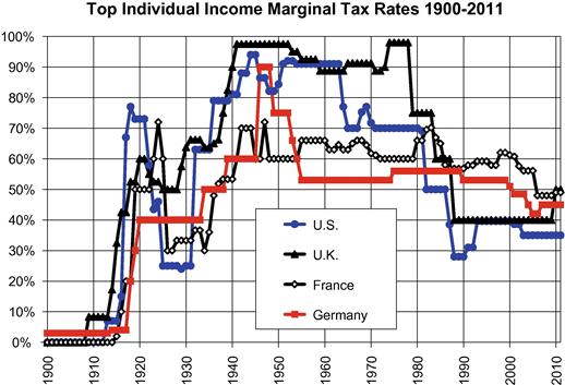
Figure 1 Top Marginal income tax rates in the US, UK, France, Germany. This figure, taken from Piketty et al. (2011), depicts the top marginal individual income tax rate in the US, UK, France, Germany since 1900. The tax rate includes only the top statutory individual income tax rate applying to ordinary income with no tax preference. State income taxes are not included in the case of the United States. For France, we include both the progressive individual income tax and the flat rate tax “Contribution Sociale Généralisée.”
As we shall see, optimal nonlinear labor income tax theory derives a simple formula for the optimal tax rate at the top of the earnings distribution. We will not deal however with the dynamic redistributive impact of tax progressivity through capital and wealth taxation, which might well have been larger historically than its static impact, as suggested by the recent literature on the long run evolution of top income shares.11
Transfers. The secular rise in taxes has been used primarily to fund growing public goods and social transfers in four broad areas: education, health care, retirement and disability, and income security (see Table 1). Indeed, aside from those four areas, government spending (as a fraction of GDP) has not grown substantially since 1900. All advanced economies provide free public education at the primary and secondary level, and heavily subsidized (and often almost free) higher education.12 All advanced economies except the United States provide universal public health care (the United States provides public health care to the old and the poor through the Medicare and Medicaid programs respectively, which taken together happen to be more expensive than most universal health care systems), as well as public retirement and disability benefits. Income security programs include unemployment benefits, as well as an array of means-tested transfers (both cash and in-kind). They are a relatively small fraction of total transfers (typically less than 5% of GDP, out of a total around 25–35% of GDP for social spending as a whole; see Table 1).
Table 1
Public Spending in OECD Countries (2000–2010, Percent of GDP)
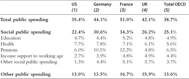
Notes and sources: OECD Economic Outlook 2012, Annex Tables 25–31; Adema et al., 2011, Table 1.2; Education at a Glance, OECD 2011, Table B4.1. Total public spending includes all government outlays (except net debt interest payments). Other social public spending includes social services to the elderly and the disabled, family services, housing and other social policy areas (see Adema et al., 2011, p.21). We report 2000–2010 averages so as to smooth business cycle variations. Note that tax to GDP ratios are a little bit lower than spending to GDP ratios for two reasons: (a) governments typically run budget deficits (which can be large, around 5–8 GDP points during recessions), (b) governments get revenue from non-tax sources (such as user fees, profits from government owned firms, etc.).
Education, family benefits, and health care government spending are approximately a demogrant, that is, a transfer of equal value for all individuals in expectation over a lifetime.13 In contrast, retirement benefits are approximately proportional to lifetime labor income in most countries.14 Finally, income security programs are targeted to lower income individuals. This is therefore the most redistributive component of the transfer system. Income security programs often take the form of in-kind benefits such as subsidized housing, subsidized food purchases (e.g., food stamps and free lunches at school in the United States), or subsidized health care (e.g., Medicaid in the United States). They are also often targeted to special groups such as the unemployed (unemployment insurance), the elderly or disabled with no resources (for example Supplemental Security Income in the United States). Means-tested cash transfer programs for “able bodied” individuals are only a small fraction of total transfers. To a large extent, the rise of the modern welfare state is the rise of universal access to “basic goods” (education, health, retirement and social insurance), and not the rise of cash transfers (see e.g., Lindert, 2004).15
In recent years, traditional means-tested cash welfare programs have been partly replaced by in-work benefits. The shift has been particularly large in the United States and the United Kingdom. Traditional means-tested programs are L-shaped with income. They provide the largest benefits to those with no income and those benefits are then phased-out at high rates for those with low earnings. Such a structure concentrates benefits among those who need them most. At the same time and as we shall see, these phase-outs discourage work as they create large implicit taxes for low earners. In contrast, in-work benefits are inversely U-shaped, first rising and then declining with earnings. Benefits are nil for those with no earnings and concentrated among low earners before being phased-out. Such a structure encourages work but fails to provide support to those with no earnings, arguably those most in need of support.
Overall, all transfers taken together are fairly close to a demogrant, i.e., are about constant with income. Hence, the optimal linear tax model with a demogrant is a reasonable first order approximation of actual tax systems and is useful to understand how the level of taxes and transfers should be set. At a finer level, there is variation in the profile of transfers. Such a profile can be analyzed using the more complex nonlinear optimal tax models.
Budget Set. The budget set relating pre-tax and pre-transfers earnings to post-tax post-transfer disposable income summarizes the net impact of the tax and transfer system. The slope of the budget set captures the marginal incentive to work. Figure 2 depicts the budget set for a single parent with two children in France and the United States. The figure includes all payroll taxes and the income tax, on the tax side. It includes means-tested transfer programs (TANF and Food Stamps in the United States, and the minimum income—RSA for France) and tax credits (the Earned Income Tax Credit and the Child Tax Credit in the United States, in-work benefit Prime pour l’Emploi and cash family benefits in France). France offers more generous support to single parents with no earnings but the French tax and transfer system imposes higher implicit taxes on work.16 As mentioned above, optimal nonlinear income tax theory precisely tries to assess what is the most desirable profile for taxes and transfers.
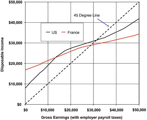
Figure 2 Tax/transfer system in the US and France, 2010, single parent with two children. The figure depicts the budget set for a single parent with two children in France and the United States (exchange rate 1 Euro = $1.3). The figure includes payroll taxes and income taxes on the tax side. It includes means-tested transfer programs (TANF and Food stamps in the United States, and the minimum income–RSA for France) and tax credits (the Earned Income Tax Credit and the Child Tax Credit in the United States, in-work benefit Prime pour l’Emploi and cash family benefits in France). Note that this graph ignores important elements. First, the health insurance Medicaid program in the United States is means tested and adds a significant layer of implicit taxation on low income work. France offers universal health insurance which does not create any additional implicit tax on work. Second, the graph ignores in-kind benefits for children such as subsidized child care and free pre-school kindergarten in France that have significant value for working single parents. Such programs barely exist in the United States. Third, the graph ignores temporary unemployment insurance benefits which depend on previous earnings for those who have become recently unemployed and which are significantly more generous in France both in level and duration.
Policy Debate. At the center of the political debate on labor income taxation and transfers is the equity-efficiency trade off. The key argument in favor of redistribution through progressive taxation and generous transfers is that social justice requires the most successful to contribute to the economic well being of the less fortunate. The reasons why society values such redistribution from high to low incomes are many. As we shall see, the standard utilitarian approach posits that marginal utility of consumption decreases with income so that a more equal distribution generates higher social welfare. Another and perhaps more realistic reason is that differences in earnings arise not only from differences in work behavior (over which individuals have control) but also from differences in innate ability or family background or sheer luck (over which individuals have little control). The key argument against redistribution through taxes and transfers is efficiency. Taxing the rich to fund means-tested programs for the poor reduces the incentives to work both among the rich and among transfer recipients. In the standard optimal tax theory, such responses to taxes and transfers are costly solely because of their effect on government finances.
Do Economists Matter? The academic literature in economics does play a role, although often an indirect one, in shaping the debate on tax and transfer policy. In the 1900–1910s, when modern progressive income taxes were created, economists appear to have played a role, albeit a modest one. Utilitarian economists like Jevons, Edgeworth, and Marshall had long argued that the principles of marginal utility and equal sacrifice push in favor of progressive tax rates (see e.g., Edgeworth, 1897)—but such theoretical results had little impact on the public debate. Applied economists like Seligman wrote widely translated and read books and reports (see e.g., Seligman, 1911) arguing that progressive income taxation was not only fair but also economically efficient and administratively manageable.17 Such arguments expressed in terms of practical economic and administrative rationality helped to convince reluctant mainstream economists in many countries that progressive income taxation was worth considering.18
In the 1920–1940s, the rise of top tax rates seems to have been the product of public debate and political conflict—in the context of chaotic political, financial, and social situations—rather than the outcome of academic arguments. It is worth noting, however, that a number of US economists of the time, e.g., Irving Fisher, then president of the American Economic Association, repeatedly argued that concentration of income and wealth was becoming as dangerously excessive in America as it had been for a long time in Europe, and called for steep tax progressivity (see e.g., Fisher, 1919). It is equally difficult to know whether economists had a major impact on the great reversal in top tax rates that occurred in the 1970–1980s during the Thatcher and Reagan conservative revolutions in Anglo-Saxon countries. The influential literature showing that top tax rate cuts can generate large responses of reported taxable income came after top tax rate cuts (e.g., Feldstein, 1995).
Today, most governments also draw on the work of commissions, panels, or reviews to justify tax and transfer reforms. Such reviews often play a big role in the public debate. They are sometimes commissioned by the government itself (e.g., the President’s Advisory Panel on Federal Tax Reform in the United States, US Treasury, 2005), by independent policy research institutes (e.g., the Mirrlees review on Reforming the Tax System for the 21st Century in the United Kingdom, Mirrlees (2010,2011)), or proposed by independent academics (e.g., Landais et al., 2011 for France). Such reviews always involve tax scholars who draw on the academic economic literature to shape their recommendations.19 The press also consults tax scholars to judge the merits of reforms proposed by politicians, and tax scholars naturally use findings from the academic literature when voicing their views.
2.2 History of the Field of Optimal Income Taxation
We offer here only a brief overview covering solely optimal income taxation.20 The modern analysis of optimal income taxation started with Mirrlees (1971) who rigorously posed and solved the problem. He considered the maximization of a social welfare function based on individual utilities subject to a government budget constraint and incentive constraints arising from individuals’ labor supply responses to the tax system.21 Formally, in the Mirrlees model, people differ solely through their skill (i.e., their wage rate). The government wants to redistribute from high skill to low skill individuals but can only observe earnings (and not skills). Hence, taxes and transfers are based on earnings, leading to a non-degenerate equity-efficiency trade off.
Mirrlees (1971) had an enormous theoretical influence in the development of contract and information theory, but little influence in actual policy making as the general lessons for optimal tax policy were few. The most striking and discussed result was the famous zero marginal tax rate at the top. This zero-top result was established by Sadka (1976) and Seade (1977). In addition, if the minimum earnings level is positive with no bunching of individuals at the bottom, the marginal tax rate is also zero at the bottom (Seade, 1977). A third result obtained by Mirrlees (1971) and Seade (1982) was that the optimal marginal tax rate is never negative if the government values redistribution from high to low earners.
Stiglitz (1982) developed the discrete version of the Mirrlees (1971) model with just two skills. In this discrete case, the marginal tax rate on the top skill is zero making the zero-top result loom even larger than in the continuous model of Mirrlees (1971). That likely contributed to the saliency of the zero-top result. The discrete model is useful to understand the problem of optimal taxation as an information problem generating an incentive compatibility constraint for the government. Namely, the tax system must be set up so that the high skill type does not want to work less and mimic the low skill type. This discrete model is also widely used in contract theory and industrial organization. However, this discrete model has limited use for actual tax policy recommendations because it is much harder to obtain formulas expressed in terms of sufficient statistics or put realistic numbers in the discrete two skill model than in the continuous model.22
Atkinson and Stiglitz (1976) derived the very important and influential result that under separability and homogeneity assumptions on preferences, differentiated commodity taxation is not useful when earnings can be taxed nonlinearly. This famous result was influential both for shaping the field of optimal tax theory and in tax policy debates. Theoretically, it contributed greatly to shift the theoretical focus toward optimal nonlinear taxation and away from the earlier Diamond and Mirrlees (1971) model of differentiated commodity taxation (itself based on the original Ramsey (1927) contribution). Practically, it gave a strong rationale for eliminating preferential taxation of necessities on redistributive grounds, and using instead a uniform value-added-tax combined with income-based transfers and progressive income taxation. Even more importantly, the Atkinson and Stiglitz (1976) result has been used to argue against the taxation of capital income and in favor of taxing solely earnings or consumption.
The optimal linear tax problem is technically simpler and it was known since at least Ramsey (1927) that the optimum tax rate can be expressed in terms of elasticities. Sheshinski (1972) is the first modern treatment of the optimal linear income tax problem. It was recognized early that labor supply elasticities play a key role in the optimal linear income tax rate. However, because of the disconnect between the nonlinear income tax analysis and the linear tax analysis, no systematic attempt was made to express nonlinear tax formulas in terms of estimable “sufficient statistics” until relatively recently.
Atkinson (1995), Diamond (1998), Piketty (1997), Saez (2001) showed that the optimal nonlinear tax formulas can also be expressed relatively simply in terms of elasticities.23 This made it possible to connect optimal income tax theory to the large empirical literature estimating behavioral responses to taxation.
Diamond (1980) considered an optimal tax model with participation labor supply responses, the so-called extensive margin (instead of the intensive margin of the Mirrlees, 1971). He showed that the optimal marginal tax rate can actually be negative in that case. As we shall see, this model with extensive margins has received renewed attention in the last decade. Saez (2002a) developed simple elasticity-based formulas showing that a negative marginal tax rate (i.e., a subsidy for work) is optimal at the bottom in such an extensive labor supply model.
With hindsight, it may seem obvious that the quest for theoretical results in optimal income tax theory with broad applicability was doomed to yield only limited results. We know that the efficiency costs of taxation depend on the size of behavioral responses to taxes and hence that optimal tax systems are going to be heavily dependent on the size of those empirical parameters.
In this handbook chapter, in addition to emphasizing connections between theory and practical recommendations, we also want to flag clearly areas, where we feel that the theory fails to provide useful practical policy guidance. Those failures arise both because of limitations of empirical work and limitations of the theoretical framework. We discuss limitations of the standard utilitarian framework in Section 7. Another theoretical limitation arises because of behavioral considerations, i.e., the fact that individuals do not behave according to the standard utility maximization model, due to psychological effects and cognitive limitations. Such behavioral effects naturally affect the analysis and have generated an active literature both theoretical and empirical that we do not cover here (see e.g., Congdon, Mullainathan, & Schwartzstein, 2012 and the chapter by Chetty and Finkelstein in this volume for applications of behavioral economics to public economics).
3 Conceptual Background
3.1 Utilitarian Social Welfare Objective
The dominant approach in normative public economics is to base social welfare on individual utilities. The simplest objective is to maximize the sum of individual utilities, the so-called utilitarian (or Benthamite) objective.24
Fixed Earnings. To illustrate the key ideas, consider a simple economy with a population normalized to one and an exogenous pre-tax earnings distribution with cumulative distribution function ![]() , i.e.,
, i.e., ![]() is the fraction of the population with pre-tax earnings below
is the fraction of the population with pre-tax earnings below ![]() . Let us assume that all individuals have the same utility function
. Let us assume that all individuals have the same utility function ![]() increasing and concave in disposable income
increasing and concave in disposable income ![]() (since there is only one period, disposable income is equal to consumption). Disposable income is pre-tax earnings minus taxes on earnings so that
(since there is only one period, disposable income is equal to consumption). Disposable income is pre-tax earnings minus taxes on earnings so that ![]() . The government chooses the tax function
. The government chooses the tax function ![]() to maximize the utilitarian social welfare function:
to maximize the utilitarian social welfare function:
![]()
where ![]() is an exogenous revenue requirement for the government and
is an exogenous revenue requirement for the government and ![]() is the Lagrange multiplier of the government budget constraint. As incomes
is the Lagrange multiplier of the government budget constraint. As incomes ![]() are fixed, this is a point-wise maximization problem and the first order condition in
are fixed, this is a point-wise maximization problem and the first order condition in ![]() is simply:
is simply:
![]()
Hence, utilitarianism with fixed earnings and concave utility implies full redistribution of incomes. The government confiscates 100% of earnings, funds its revenue requirement, and redistributes the remaining tax revenue equally across individuals. This result was first established by Edgeworth (1897). The intuition for this strong result is straightforward. With concave utilities, marginal utility ![]() is decreasing with
is decreasing with ![]() . Hence, if
. Hence, if ![]() then
then ![]() and it is desirable to transfer resources from the person consuming
and it is desirable to transfer resources from the person consuming ![]() to the person consuming
to the person consuming ![]() .
.
Generalized social welfare functions of the form ![]() where
where ![]() is increasing and concave are also often considered. The limiting case where
is increasing and concave are also often considered. The limiting case where ![]() is infinitely concave is the Rawlsian (or maxi-min ) criterion where the government’s objective is to maximize the utility of the most disadvantaged person, i.e., maximize the minimum utility (maxi-min). In this simple context with fixed incomes, all those objectives also leads to 100% redistribution as in the standard utilitarian case.
is infinitely concave is the Rawlsian (or maxi-min ) criterion where the government’s objective is to maximize the utility of the most disadvantaged person, i.e., maximize the minimum utility (maxi-min). In this simple context with fixed incomes, all those objectives also leads to 100% redistribution as in the standard utilitarian case.
Finally, with heterogeneous utility functions ![]() across individuals, the utilitarian optimum is such that
across individuals, the utilitarian optimum is such that ![]() is constant over the population. Comparing the levels of marginal utility of consumption conditional on disposable income
is constant over the population. Comparing the levels of marginal utility of consumption conditional on disposable income ![]() across people with different preferences raises difficult issues of interpersonal utility comparisons. There might be legitimate reasons, such as required health expenses due to medical conditions, that make marginal utility of consumption higher for some people than for others even conditional on after-tax income
across people with different preferences raises difficult issues of interpersonal utility comparisons. There might be legitimate reasons, such as required health expenses due to medical conditions, that make marginal utility of consumption higher for some people than for others even conditional on after-tax income ![]() . Another legitimate reason would be the number of dependent children. Absent such need-based legitimate reasons, it does not seem feasible nor reasonable for society to discriminate in favor of those with high marginal utility of consumption (e.g., those who really enjoy consumption) against those with low marginal utility of consumption (e.g., those less able to enjoy consumption). This is not feasible because marginal utility of consumption cannot be observed and compared across individuals. Even if marginal utility were observable, it is unlikely that such discrimination would be acceptable to society (see our discussion in Section 6).
. Another legitimate reason would be the number of dependent children. Absent such need-based legitimate reasons, it does not seem feasible nor reasonable for society to discriminate in favor of those with high marginal utility of consumption (e.g., those who really enjoy consumption) against those with low marginal utility of consumption (e.g., those less able to enjoy consumption). This is not feasible because marginal utility of consumption cannot be observed and compared across individuals. Even if marginal utility were observable, it is unlikely that such discrimination would be acceptable to society (see our discussion in Section 6).
Therefore, it seems fair for the government to consider social welfare functions such that social marginal utility of consumption is the same across individuals conditional on disposable income. In the fixed earnings case, this means that the government can actually ignore individual utilities and use a “universal” social utility function ![]() to evaluate social welfare. The concavity of
to evaluate social welfare. The concavity of ![]() then reflects society’s value for redistribution rather than directly individual marginal utility of consumption.25 We will come back to this important point later on.
then reflects society’s value for redistribution rather than directly individual marginal utility of consumption.25 We will come back to this important point later on.
Endogenous Earnings. Naturally, the result of complete redistribution with concave utility depends strongly on the assumption of fixed earnings. In the real world, complete redistribution would certainly greatly diminish incentives to work and lead to a decrease in pre-tax earnings. Indeed, the goal of optimal income tax theory has been precisely to extend the basic model to the case with endogenous earnings (Vickrey, 1945 and Mirrlees, 1971). Taxation then generates efficiency costs as it reduces earnings, and the optimal tax problem becomes a non-trivial equity-efficiency trade off. Hence, with utilitarianism, behavioral responses are the sole factor preventing complete redistribution. In reality, society might also oppose complete redistribution on fairness grounds even setting aside the issue of behavioral responses. We come back to this limitation of utilitarianism in Section 6.
Let us therefore now assume that earnings are determined by labor supply and that individuals derive disutility from work. Individual ![]() has utility
has utility ![]() increasing in
increasing in ![]() but decreasing with earnings
but decreasing with earnings ![]() . In that world, 100% taxation would lead everybody to completely stop working, and hence is not desirable.
. In that world, 100% taxation would lead everybody to completely stop working, and hence is not desirable.
Let us consider general social welfare functions of the type:
![]()
where ![]() are Pareto weights independent of individual choices
are Pareto weights independent of individual choices ![]() and
and ![]() an increasing transformation of utilities, and
an increasing transformation of utilities, and ![]() is the distribution of individuals. The combination of arbitrary Pareto weights
is the distribution of individuals. The combination of arbitrary Pareto weights ![]() and a social welfare function
and a social welfare function ![]() allows us to be fully general for the moment. We denote by
allows us to be fully general for the moment. We denote by
![]()
the social marginal welfare weight on individual ![]() , with
, with ![]() the multiplier of the government budget constraint.
the multiplier of the government budget constraint.
Intuitively, ![]() measures the dollar value (in terms of public funds) of increasing consumption of individual
measures the dollar value (in terms of public funds) of increasing consumption of individual ![]() by $1. With fixed earnings, any discrepancy in the
by $1. With fixed earnings, any discrepancy in the ![]() ’s across individuals calls for redistribution as it increases social welfare to transfer resources from those with lower
’s across individuals calls for redistribution as it increases social welfare to transfer resources from those with lower ![]() ’s toward those with higher
’s toward those with higher ![]() ’s. Hence, absent efficiency concerns, the government should equalize all the
’s. Hence, absent efficiency concerns, the government should equalize all the ![]() ’s.26 With endogenous earnings, the
’s.26 With endogenous earnings, the ![]() ’s will no longer be equalized at the optimum. As we shall see, social preferences for redistribution enter optimal tax formulas solely through the
’s will no longer be equalized at the optimum. As we shall see, social preferences for redistribution enter optimal tax formulas solely through the ![]() weights.
weights.
Under the utilitarian objective, ![]() is directly proportional to the marginal utility of consumption. Under the Rawlsian criterion, all the
is directly proportional to the marginal utility of consumption. Under the Rawlsian criterion, all the ![]() are zero, except for the most disadvantaged.
are zero, except for the most disadvantaged.
In the simpler case with no income effects on labor supply, i.e., where utility functions take the quasi-linear form ![]() with
with ![]() increasing and concave and
increasing and concave and ![]() increasing and convex, the labor supply decision does not depend on non-labor income (see Section 3.3) and the average of
increasing and convex, the labor supply decision does not depend on non-labor income (see Section 3.3) and the average of ![]() across all individuals is equal to one. This can be seen as follows. The government is indifferent between one more dollar of tax revenue and redistributing $1 to everybody (as giving one extra dollar lump-sum does not generate any behavioral response). The value of giving $1 extra to person
across all individuals is equal to one. This can be seen as follows. The government is indifferent between one more dollar of tax revenue and redistributing $1 to everybody (as giving one extra dollar lump-sum does not generate any behavioral response). The value of giving $1 extra to person ![]() , in terms of public funds, is
, in terms of public funds, is ![]() so that the value of redistributing $1 to everybody is
so that the value of redistributing $1 to everybody is ![]() .
.
3.2 Fallacy of the Second Welfare Theorem
The second welfare theorem seems to provide a strikingly simple theoretical solution to the equity-efficiency trade off. Under standard perfect market assumptions, the second welfare theorem states that any Pareto efficient outcome can be reached through a suitable set of lump-sum taxes that depend on exogenous characteristics of each individual (e.g., intrinsic abilities or other endowments or random shocks), and the subsequent free functioning of markets with no additional government interference. The logic is very simple. If some individuals have better earnings ability than others and the government wants to equalize disposable income, it is most efficient to impose a tax (or a transfer) based on earnings ability and then let people keep 100% of their actual earnings at the margin.27
In standard models, it is assumed that the government cannot observe earnings abilities but only realized earnings. Hence, the government has to base taxes and transfers on actual earnings only, which distort earnings and create efficiency costs. This generates an equity-efficiency trade off. This informational structure puts optimal tax analysis on sound theoretical grounds and connects it to mechanism design. While this is a theoretically appealing reason for the failure of the second welfare theorem, in our view, there must be a much deeper reason for governments to systematically use actual earnings rather than proxies for ability in real tax systems.
Indeed, standard welfare theory implies that taxes and transfers should depend on any characteristic correlated with earnings ability in the optimal tax system. If the characteristic is immutable, then average social marginal utilities across groups with different characteristics should be perfectly equalized. Even if the characteristic is manipulable, it should still be used in the optimal system (see Section 6.1). In reality, actual income tax or transfer systems depend on very few other characteristics than income. Those characteristics, essentially family situation or disability status, seem limited to factors clearly related to need.28
The traditional way to resolve this puzzle has been to argue that there are additional horizontal equity concerns that prevent the government from using non-income characteristics for tax purposes (see e.g., Atkinson and Stiglitz (1980) pp. 354–5). Recently, Mankiw and Weinzierl (2010) argue that this represents a major failure of the standard social welfare approach. This shows that informational concerns and observability is not the overwhelming reason for basing taxes and transfers almost exclusively on income. This has two important consequences.
First, finding the most general mechanism compatible with the informational set of the government—as advocated for example in the New Dynamic Public Finance literature (see Kocherlakota, 2010 for a survey)—might not be very useful for understanding actual tax problems. Such an approach can provide valuable theoretical insights and results but is likely to generate optimal tax systems that are so fundamentally different from actual tax systems that they are not implementable in practice. It seems more fruitful practically to assume instead exogenously that the government can only use a limited set of tax tools, precisely those that are used in practice, and consider the optimum within the set of real tax systems actually used. In most of this chapter, we therefore pursue this “simple tax structure” approach.29
Second, it would certainly be useful to make progress on understanding what concepts of justice or fairness could lead the government to use only a specific subset of taxes and deliberately ignore other tools—such as taxes based on non-income characteristics correlated with ability—that would be useful to maximize standard utilitarian social welfare functions. We will come back to those important issues in Section 6.1 where we study tagging and in Section 7 where we consider alternatives to utilitarianism.
3.3 Labor Supply Concepts
In this chapter, we always consider a population of measure one of individuals. In most sections, individuals have heterogeneous preferences over consumption and earnings. Individual ![]() utility is denoted by
utility is denoted by ![]() and is increasing in consumption
and is increasing in consumption ![]() and decreasing in earnings
and decreasing in earnings ![]() as earnings require labor supply. Following Mirrlees (1971), in most models, heterogeneity in preferences is due solely to differences in wage rates
as earnings require labor supply. Following Mirrlees (1971), in most models, heterogeneity in preferences is due solely to differences in wage rates ![]() where utility functions take the form
where utility functions take the form ![]() where
where ![]() is labor supply needed to earn
is labor supply needed to earn ![]() . Our formulation
. Our formulation ![]() is more general and can capture both heterogeneity in ability as well as heterogeneity in preferences. As mentioned earlier, we believe that heterogeneity is an important element of the real world and optimal tax results should be reasonably robust to it.
is more general and can capture both heterogeneity in ability as well as heterogeneity in preferences. As mentioned earlier, we believe that heterogeneity is an important element of the real world and optimal tax results should be reasonably robust to it.
To derive labor supply concepts, we consider a linear tax system with a tax rate ![]() combined with a lump sum demogrant
combined with a lump sum demogrant ![]() so that the budget constraint of each individual is
so that the budget constraint of each individual is ![]() .
.
Intensive Margin. Let us focus first on the intensive labor supply margin, that is on the choice of how much to earn conditional on working. Individual ![]() chooses
chooses ![]() to maximize
to maximize ![]() which leads to the first order condition
which leads to the first order condition
![]()
which defines implicitly the individual uncompensated (also called Marshallian) earnings supply function ![]() .
.
The effect of ![]() on
on ![]() defines the uncompensated elasticity
defines the uncompensated elasticity![]() of earnings with respect to the net-of-tax rate
of earnings with respect to the net-of-tax rate![]() . The effect of
. The effect of ![]() on
on ![]() defines the income effect
defines the income effect![]() . If leisure is a normal good, an assumption we make from now on, then
. If leisure is a normal good, an assumption we make from now on, then ![]() as receiving extra non-labor income induces the individual to consume both more goods and more leisure.
as receiving extra non-labor income induces the individual to consume both more goods and more leisure.
Finally, one can also define the compensated (also called Hicksian) earnings supply function ![]() as the earnings level that minimizes the cost necessary to reach utility
as the earnings level that minimizes the cost necessary to reach utility ![]() .30 The effect of
.30 The effect of ![]() on
on ![]() keeping
keeping ![]() constant defines the compensated elasticity
constant defines the compensated elasticity![]() of earnings with respect to the net-of-tax rate
of earnings with respect to the net-of-tax rate![]() . The compensated elasticity is always positive.
. The compensated elasticity is always positive.
The Slutsky equation relates those parameters ![]() . To summarize we have:
. To summarize we have:
 (1)
(1)
In the long-run process of development over the last century in the richest countries, wage rates have increased by a factor of five. Labor supply measured in hours of work has declined only very slightly (Ramey & Francis, 2009). If preferences for consumption and leisure have not changed, this implies that the uncompensated elasticity is close to zero. This does not mean however that taxes would have no effect on labor supply as a large fraction of taxes are rebated as transfers (see our discussion in Section 2). Therefore, on average, taxes are more similar to a compensated wage rate decrease than an uncompensated wage rate decrease. If income effects are large, government taxes and transfers could still have a large impact on labor supply.
Importantly, although we have defined those labor supply concepts for a linear tax system, they continue to apply in the case of a nonlinear tax system by considering the linearized budget at the utility maximizing point. In that case, we replace ![]() by the marginal tax rate
by the marginal tax rate ![]() and we replace
and we replace ![]() by virtual income defined as the non-labor income that the individual would get if her earnings were zero and she could stay on the virtual linearized budget. Formally
by virtual income defined as the non-labor income that the individual would get if her earnings were zero and she could stay on the virtual linearized budget. Formally ![]() .
.
Hence, the marginal tax rate ![]() reduces the marginal benefit of earning an extra dollar and reduces labor supply through substitution effects, conditional on the tax level
reduces the marginal benefit of earning an extra dollar and reduces labor supply through substitution effects, conditional on the tax level ![]() . The income tax level
. The income tax level ![]() increases labor supply through income effects. In net, taxes (with
increases labor supply through income effects. In net, taxes (with ![]() and
and ![]() ) hence have an ambiguous effect on labor supply while transfers (with
) hence have an ambiguous effect on labor supply while transfers (with ![]() and
and ![]() ) have an unambiguously negative effect on labor supply.
) have an unambiguously negative effect on labor supply.
Extensive Margin. In practice, there are fixed costs of work (e.g., searching for a job, finding alternative child care for parents, loss of home production, transportation costs, etc.). This can be captured in the basic model by assuming that choosing ![]() (as opposed to
(as opposed to ![]() ) involves a discrete cost
) involves a discrete cost ![]() .
.
It is possible to consider a pure extensive margin model by assuming that individual ![]() can either not work (and earn zero) or work and earn
can either not work (and earn zero) or work and earn ![]() where
where ![]() is fixed to individual
is fixed to individual ![]() and reflects her earning potential. Assume that utility is linear, i.e.,
and reflects her earning potential. Assume that utility is linear, i.e., ![]() where
where ![]() is net-of-tax income,
is net-of-tax income, ![]() is the cost of work and
is the cost of work and ![]() is a work dummy. In that case, individual
is a work dummy. In that case, individual ![]() works if and only if
works if and only if ![]() , i.e., if
, i.e., if ![]() where
where ![]() .
. ![]() is the participation tax rate, defined as the fraction of earnings taxed when the individual goes from not working and earning zero to working and earning
is the participation tax rate, defined as the fraction of earnings taxed when the individual goes from not working and earning zero to working and earning ![]() . Therefore, the decision to work depends on the net-of-tax participation tax rate
. Therefore, the decision to work depends on the net-of-tax participation tax rate ![]() .
.
To summarize, there are three key concepts for any tax and transfer system ![]() . First, the transfer benefit with zero earnings
. First, the transfer benefit with zero earnings ![]() , sometimes called demogrant or lump-sum grant. Second, the marginal tax rate (or phasing-out rate)
, sometimes called demogrant or lump-sum grant. Second, the marginal tax rate (or phasing-out rate) ![]() : The individual keeps
: The individual keeps ![]() for an additional $1 of earnings.
for an additional $1 of earnings. ![]() is the key concept for the intensive labor supply choice. Third, the participation tax rate
is the key concept for the intensive labor supply choice. Third, the participation tax rate ![]() : The individual keeps a fraction
: The individual keeps a fraction ![]() of his earnings when going from zero earnings to earnings
of his earnings when going from zero earnings to earnings ![]() .
. ![]() is the key concept for the extensive labor supply choice. Finally, note that
is the key concept for the extensive labor supply choice. Finally, note that ![]() integrates both the means-tested transfer program and the income tax that funds such transfers and other government spending. In practice transfer programs and taxes are often administered separately. The break even earnings point
integrates both the means-tested transfer program and the income tax that funds such transfers and other government spending. In practice transfer programs and taxes are often administered separately. The break even earnings point ![]() is the point at which
is the point at which ![]() . Above the break even point,
. Above the break even point, ![]() which encourages labor supply through income effects. Below the break even point,
which encourages labor supply through income effects. Below the break even point, ![]() which discourages labor supply through income effects.
which discourages labor supply through income effects.
Tax Reform Welfare Effects and Envelope Theorem. A key element of optimal tax analysis is the evaluation of the welfare effects of small tax reforms. Consider a nonlinear tax ![]() . Individual
. Individual ![]() chooses
chooses ![]() to maximize
to maximize ![]() , leading to the first order condition
, leading to the first order condition ![]() . Consider now a small reform
. Consider now a small reform ![]() of the nonlinear tax schedule. The effect on individual utility
of the nonlinear tax schedule. The effect on individual utility ![]() is
is
![]()
where ![]() is the behavioral response of the individual to the tax reform and the second equality is obtained because of the first order condition
is the behavioral response of the individual to the tax reform and the second equality is obtained because of the first order condition ![]() . This is a standard application of the envelope theorem. As
. This is a standard application of the envelope theorem. As ![]() maximizes utility, any small change
maximizes utility, any small change ![]() has no first order effect on individual utility. As a result, behavioral responses can be ignored and the change in individual welfare is simply given by the mechanical effect of the tax reform on the individual budget multiplied by the marginal utility of consumption.
has no first order effect on individual utility. As a result, behavioral responses can be ignored and the change in individual welfare is simply given by the mechanical effect of the tax reform on the individual budget multiplied by the marginal utility of consumption.
4 Optimal Linear Taxation
4.1 Basic Model
Linear labor income taxation simplifies considerably the exposition but captures the key equity-efficiency trade off. Sheshinski (1972) offered the first modern treatment of optimal linear income taxation following the nonlinear income tax analysis of Mirrlees (1971). Both the derivation and the optimal formulas are also closely related to the more complex nonlinear case. It is therefore pedagogically useful to start with the linear case where the government uses a linear tax at rate ![]() to fund a demogrant
to fund a demogrant ![]() (and additional non-transfer spending
(and additional non-transfer spending ![]() taken as exogenous).31
taken as exogenous).31
Summing the Marshallian individual earnings functions ![]() , we obtain aggregate earnings which depend upon
, we obtain aggregate earnings which depend upon ![]() and
and ![]() and can be denoted by
and can be denoted by ![]() . The government’s budget constraint is
. The government’s budget constraint is ![]() , which defines implicitly
, which defines implicitly ![]() as a function of
as a function of ![]() only (as we assume that
only (as we assume that ![]() is fixed exogenously). Hence, we can express aggregate earnings as a sole function of
is fixed exogenously). Hence, we can express aggregate earnings as a sole function of ![]() . The tax revenue function
. The tax revenue function ![]() has an inverted U-shape. It is equal to zero both when
has an inverted U-shape. It is equal to zero both when ![]() (no taxation) and when
(no taxation) and when ![]() (complete taxation) as 100% taxation entirely discourages labor supply. This curve is popularly called the Laffer curve although the concept of the revenue curve has been known since at least Dupuit (1844). Let us denote by
(complete taxation) as 100% taxation entirely discourages labor supply. This curve is popularly called the Laffer curve although the concept of the revenue curve has been known since at least Dupuit (1844). Let us denote by ![]() the elasticity of aggregate earnings with respect to the net-of-tax rate. The tax rate
the elasticity of aggregate earnings with respect to the net-of-tax rate. The tax rate ![]() maximizing tax revenue is such that
maximizing tax revenue is such that ![]() , i.e.,
, i.e., ![]() . Hence, we can express
. Hence, we can express ![]() as a sole function of
as a sole function of ![]() :
:
![]() (2)
(2)
Let us now consider the maximization of a general social welfare function. The demogrant ![]() evenly distributed to everybody is equal to
evenly distributed to everybody is equal to ![]() and hence disposable income for individual
and hence disposable income for individual ![]() is
is ![]() (recall that population size is normalized to one). Therefore, the government chooses
(recall that population size is normalized to one). Therefore, the government chooses ![]() to maximize
to maximize
![]()
Using the envelope theorem from the choice of ![]() in the utility maximization problem of individual
in the utility maximization problem of individual ![]() , the first order condition for the government is simply
, the first order condition for the government is simply
![]()
The first term in the square brackets ![]() reflects the mechanical effect of increasing taxes (and the demogrant) absent any behavioral response. This effect is positive when individual income
reflects the mechanical effect of increasing taxes (and the demogrant) absent any behavioral response. This effect is positive when individual income ![]() is less than average income
is less than average income ![]() . The second term
. The second term ![]() reflects the efficiency cost of increasing taxes due to the aggregate behavioral response. This is an efficiency cost because such behavioral responses have no first order positive welfare effect on individuals but have a first order negative effect on tax revenue.
reflects the efficiency cost of increasing taxes due to the aggregate behavioral response. This is an efficiency cost because such behavioral responses have no first order positive welfare effect on individuals but have a first order negative effect on tax revenue.
Introducing the aggregate elasticity ![]() and the “normalized” social marginal welfare weight
and the “normalized” social marginal welfare weight ![]() , we can rewrite the first order condition as:
, we can rewrite the first order condition as:
![]()
Hence, we have the following optimal linear income tax formula
![]() (3)
(3)![]()
is the average “normalized” social marginal welfare weight weighted by pre-tax incomes ![]() .
. ![]() is also the ratio of the average income weighted by individual social welfare weights
is also the ratio of the average income weighted by individual social welfare weights ![]() to the actual average income
to the actual average income ![]() . Hence,
. Hence, ![]() measures where social welfare weights are concentrated on average over the distribution of earnings. An alternative form for formula (3) often presented in the literature takes the form
measures where social welfare weights are concentrated on average over the distribution of earnings. An alternative form for formula (3) often presented in the literature takes the form ![]() where
where ![]() is the covariance between social marginal welfare weights
is the covariance between social marginal welfare weights ![]() and normalized earnings
and normalized earnings ![]() . As long as the correlation between
. As long as the correlation between ![]() and
and ![]() is negative, i.e., those with higher incomes have lower social marginal welfare weights, the optimum
is negative, i.e., those with higher incomes have lower social marginal welfare weights, the optimum ![]() is positive. Five points are worth noting about formula (3).
is positive. Five points are worth noting about formula (3).
First, the optimal tax rate decreases with the aggregate elasticity ![]() . This elasticity is a mix of substitution and income effects as an increase in the tax rate
. This elasticity is a mix of substitution and income effects as an increase in the tax rate ![]() is associated with an increase in the demogrant
is associated with an increase in the demogrant ![]() . Formally, one can show that
. Formally, one can show that ![]() where
where ![]() is the average of the individual uncompensated elasticities
is the average of the individual uncompensated elasticities ![]() weighted by income
weighted by income ![]() and
and ![]() is the unweighted average of individual income effects
is the unweighted average of individual income effects ![]() .32 This allows us to rewrite the optimal tax formula (3) in a slightly more structural form as
.32 This allows us to rewrite the optimal tax formula (3) in a slightly more structural form as ![]() .
.
When the tax rate maximizes tax revenue, we have ![]() and then
and then ![]() is a pure uncompensated elasticity (as the tax rate does not raise any extra revenue at the margin). When the tax rate is zero,
is a pure uncompensated elasticity (as the tax rate does not raise any extra revenue at the margin). When the tax rate is zero, ![]() is conceptually close to a compensated elasticity as taxes raised are fully rebated with no efficiency loss.33
is conceptually close to a compensated elasticity as taxes raised are fully rebated with no efficiency loss.33
Second, the optimal tax rate naturally decreases with ![]() which measures the redistributive tastes of the government. In the extreme case where the government does not value redistribution at all,
which measures the redistributive tastes of the government. In the extreme case where the government does not value redistribution at all, ![]() and hence
and hence ![]() and
and ![]() is optimal.34 In the polar opposite case where the government is Rawlsian and maximizes the lump sum demogrant (assuming the worst-off individual has zero earnings), then
is optimal.34 In the polar opposite case where the government is Rawlsian and maximizes the lump sum demogrant (assuming the worst-off individual has zero earnings), then ![]() and
and ![]() , which is the revenue maximizing tax rate from Eq. (2). As mentioned above, in that case
, which is the revenue maximizing tax rate from Eq. (2). As mentioned above, in that case ![]() is an uncompensated elasticity.
is an uncompensated elasticity.
Third and related, for a given profile of social welfare weights (or for a given degree of concavity of the utility function in the homogeneous utilitarian case), the higher the pre-tax inequality at a given ![]() , the lower
, the lower ![]() , and hence the higher the optimal tax rate. If there is no inequality, then
, and hence the higher the optimal tax rate. If there is no inequality, then ![]() and
and ![]() with a lump-sum tax
with a lump-sum tax ![]() is optimal. If inequality is maximal, i.e., nobody earns anything except for a single person who earns everything and has a social marginal welfare weight of zero, then
is optimal. If inequality is maximal, i.e., nobody earns anything except for a single person who earns everything and has a social marginal welfare weight of zero, then ![]() , again equal to the revenue maximizing tax rate.
, again equal to the revenue maximizing tax rate.
Fourth, it is important to note that, as is usual in optimal tax theory, formula (3) is an implicit formula for ![]() as both
as both ![]() and especially
and especially ![]() vary with
vary with ![]() . Under a standard utilitarian social welfare criterion with concave utility of consumption,
. Under a standard utilitarian social welfare criterion with concave utility of consumption, ![]() increases with
increases with ![]() as the need for redistribution (i.e., the variation of the
as the need for redistribution (i.e., the variation of the ![]() with
with ![]() ) decreases with the level of taxation
) decreases with the level of taxation ![]() . This ensures that formula (3) generates a unique equilibrium for
. This ensures that formula (3) generates a unique equilibrium for ![]() .
.
Fifth, formula (3) can also be used to assess tax reform. Starting from the current ![]() , the current estimated elasticity
, the current estimated elasticity ![]() , and the current welfare weight parameter
, and the current welfare weight parameter ![]() , if
, if ![]() then increasing
then increasing ![]() increases social welfare (and conversely). The tax reform approach has the advantage that it does not require knowing how
increases social welfare (and conversely). The tax reform approach has the advantage that it does not require knowing how ![]() and
and ![]() change with
change with ![]() , since it only considers local variations.
, since it only considers local variations.
Generality of the Formula. The optimal linear tax formula is very general as it applies to many alternative models for the income generating process. All that matters is the aggregate elasticity ![]() and how the government sets normalized marginal welfare weights
and how the government sets normalized marginal welfare weights ![]() . First, if the population is discrete, the same derivation and formula obviously apply. Second, if labor supply responses are (partly or fully) along the extensive margin, the same formula applies. Third, the same formula also applies in the long run when educational and human capital decisions are potentially affected by the tax rate as those responses are reflected in the long-run aggregate elasticity
. First, if the population is discrete, the same derivation and formula obviously apply. Second, if labor supply responses are (partly or fully) along the extensive margin, the same formula applies. Third, the same formula also applies in the long run when educational and human capital decisions are potentially affected by the tax rate as those responses are reflected in the long-run aggregate elasticity ![]() (see e.g., Best & Kleven, 2012).35
(see e.g., Best & Kleven, 2012).35
Random Earnings. If earnings are generated by a partly random process involving luck in addition to ability and effort, as in Varian (1980) and Eaton and Rosen (1980), formula (3) still applies as long as the social welfare objective is defined over individual expected utilities.
To see this, suppose that pre-tax income for individual ![]() is a random function of labor supply
is a random function of labor supply ![]() and an idiosyncratic luck shock
and an idiosyncratic luck shock ![]() (with distribution
(with distribution ![]() ) with
) with ![]() for simplicity. Individual
for simplicity. Individual ![]() chooses
chooses ![]() to maximize expected utility
to maximize expected utility
![]()
so that ![]() is function of
is function of ![]() and
and ![]() . The government budget implies again that
. The government budget implies again that ![]() so that
so that ![]() is also a function of
is also a function of ![]() as in the standard model (recall that
as in the standard model (recall that ![]() is an implicit function of
is an implicit function of ![]() ). The government then chooses
). The government then chooses ![]() to maximize
to maximize ![]() . This again leads to formula (3) with
. This again leads to formula (3) with ![]() the “normalized” average of
the “normalized” average of ![]() weighted by incomes
weighted by incomes ![]() where now the average is taken as a double integral over both
where now the average is taken as a double integral over both ![]() and
and ![]() .
.
Therefore, the random earnings model generates both the same equity-efficiency trade-off and the same type of optimal tax formula. This shows the robustness of the optimal linear tax approach. This robustness was not clearly apparent in the literature because of the focus on the nonlinear income tax case where the two models no longer deliver identical formulas.36
Political Economy and Median Voter. The most popular model for policy decisions among economists is the median voter model. As is well known, the median voter theorem applies for unidimensional policies and where individual preferences are single-peaked with respect to this unidimensional policy. In our framework, the unidimensional policy is the tax rate ![]() (as the demogrant
(as the demogrant ![]() is a function of
is a function of ![]() ). Each individual has single-peaked preferences about the tax rate
). Each individual has single-peaked preferences about the tax rate ![]() as
as ![]() is single-peaked with a peak such that
is single-peaked with a peak such that ![]() , i.e.,
, i.e., ![]() . Hence, the median voter is the voter with median income
. Hence, the median voter is the voter with median income ![]() . Recall that with single-peaked preferences, the median voter preferred tax rate is a Condorcet winner, i.e., wins in majority voting against any other alternative tax rate.37 Therefore, the median voter equilibrium has:
. Recall that with single-peaked preferences, the median voter preferred tax rate is a Condorcet winner, i.e., wins in majority voting against any other alternative tax rate.37 Therefore, the median voter equilibrium has:
![]() (4)
(4)
The formula implies that when the median ![]() is close to the average
is close to the average ![]() , the optimal tax rate is low because a linear tax rate achieves little redistribution (toward the median) and hence a lump-sum tax is more efficient.38 In contrast, when the median
, the optimal tax rate is low because a linear tax rate achieves little redistribution (toward the median) and hence a lump-sum tax is more efficient.38 In contrast, when the median ![]() is small relative to the average, the tax rate
is small relative to the average, the tax rate ![]() gets close to the revenue maximizing tax rate
gets close to the revenue maximizing tax rate ![]() from Eq. (2).
from Eq. (2).
Formula (4) is a particular case of formula (3) where social welfare weights are concentrated at the median so that ![]() . This shows that there is a tight connection between optimal tax theory and political economy. Political economy uses social welfare weights coming out of the political game process rather than derived from marginal utility of consumption as in the standard utilitarian tax theory but the structure of resulting tax formulas is the same (see Persson & Tabellini, 2002, chap. 24 for a comprehensive survey of political economy applied to public finance). We come back to the determination of social welfare weights in Section 6.
. This shows that there is a tight connection between optimal tax theory and political economy. Political economy uses social welfare weights coming out of the political game process rather than derived from marginal utility of consumption as in the standard utilitarian tax theory but the structure of resulting tax formulas is the same (see Persson & Tabellini, 2002, chap. 24 for a comprehensive survey of political economy applied to public finance). We come back to the determination of social welfare weights in Section 6.
Finally and as caveats, note that the median voter theory applies only to unidimensional policies so that those results do not carry over to the nonlinear income tax case. The political economy literature has also shown that real world outcomes differ substantially from median voter predictions.
4.2 Accounting for Actual Tax Rates
As we saw in Section 2, tax to GDP ratios in OECD countries are between 30% and 45% and the more economically meaningful tax to national income ratios between 35% and 50%. Quantitatively, most estimates of aggregate elasticities of taxable income are between .1 and .4 with .25 perhaps being a reasonable estimate (see Saez, Slemrod, & Giertz, 2012 for a recent survey), although there remains considerable uncertainty about these magnitudes.39
Table 2 proposes simple illustrative calculations using the optimal linear tax rate formula (3). It reports combinations of ![]() and
and ![]() in various situations corresponding to different elasticities
in various situations corresponding to different elasticities ![]() (across columns) and different social objectives (across rows). We consider three elasticity scenarios. The first one has
(across columns) and different social objectives (across rows). We consider three elasticity scenarios. The first one has ![]() which is a realistic mid-range estimate (Saez et al., 2012, Chetty, 2012). The second has
which is a realistic mid-range estimate (Saez et al., 2012, Chetty, 2012). The second has ![]() , a high range elasticity scenario. We add a third scenario with
, a high range elasticity scenario. We add a third scenario with ![]() , an extreme case well above the current average empirical estimates.
, an extreme case well above the current average empirical estimates.
Table 2
Optimal Linear Tax Rate Formula ![]()
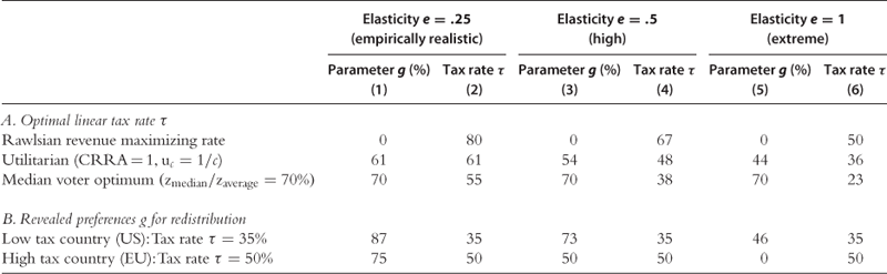
Notes: This table illustrates the use of the optimal linear tax rate formula ![]() derived in the main text. It reports combinations of
derived in the main text. It reports combinations of ![]() and g in various situations corresponding to different elasticities e (across columns) and different social objectives (across rows). Recall that g is the ratio of average earnings weighted by social marginal welfare weights to unweighted average earnings. Panel A considers the standard case where g is pinned down by a given social objective criterion and
and g in various situations corresponding to different elasticities e (across columns) and different social objectives (across rows). Recall that g is the ratio of average earnings weighted by social marginal welfare weights to unweighted average earnings. Panel A considers the standard case where g is pinned down by a given social objective criterion and ![]() is then given by the optimal tax formula. The first row is the Rawlsian criterion (or revenue maximizing tax rate) with g = 0. The second row is a utilitarian criterion with coefficient of relative risk aversion (CRRA) equal to one (social marginal welfare weights are proportional to
is then given by the optimal tax formula. The first row is the Rawlsian criterion (or revenue maximizing tax rate) with g = 0. The second row is a utilitarian criterion with coefficient of relative risk aversion (CRRA) equal to one (social marginal welfare weights are proportional to ![]() where
where ![]() is disposable income). g is endogenously determined using the actual US earnings distribution and assuming that government required spending (outside transfers) is 10% of total earnings. The third row is the median voter optimum with a median to average earnings ratio of 70% (corresponding approximately to the current US situation). Panel B considers the inverse problem of determining the social preference parameter g for a given tax rate
is disposable income). g is endogenously determined using the actual US earnings distribution and assuming that government required spending (outside transfers) is 10% of total earnings. The third row is the median voter optimum with a median to average earnings ratio of 70% (corresponding approximately to the current US situation). Panel B considers the inverse problem of determining the social preference parameter g for a given tax rate ![]() . The first row uses
. The first row uses ![]() , corresponding to a low tax country such as the United States. The second row uses
, corresponding to a low tax country such as the United States. The second row uses ![]() , corresponding to a high tax country such as a typical country from the European Union.
, corresponding to a high tax country such as a typical country from the European Union.
Panel A considers the standard case where ![]() is pinned down by a given social objective criterion and
is pinned down by a given social objective criterion and ![]() is then given by the optimal tax formula. The first row is the Rawlsian criterion (or revenue maximizing tax rate) with
is then given by the optimal tax formula. The first row is the Rawlsian criterion (or revenue maximizing tax rate) with ![]() . The second row is a utilitarian criterion with coefficient of relative risk aversion (CRRA) equal to one (social marginal welfare weights are proportional to
. The second row is a utilitarian criterion with coefficient of relative risk aversion (CRRA) equal to one (social marginal welfare weights are proportional to ![]() where
where ![]() is disposable income).40 Chetty (2006) shows that a CRRA equal to one is consistent with empirical labor supply behavior and hence a reasonable benchmark. The third row is the median voter optimum with a median to average earnings ratio of 70% (corresponding approximately to the current US distribution based on individual adult earnings from the Current Population Survey in 2010). Panel B considers the inverse problem of determining the social preference parameter
is disposable income).40 Chetty (2006) shows that a CRRA equal to one is consistent with empirical labor supply behavior and hence a reasonable benchmark. The third row is the median voter optimum with a median to average earnings ratio of 70% (corresponding approximately to the current US distribution based on individual adult earnings from the Current Population Survey in 2010). Panel B considers the inverse problem of determining the social preference parameter ![]() for a given tax rate
for a given tax rate ![]() . The first row uses
. The first row uses ![]() , corresponding to a low tax country such as the United States. The second row uses
, corresponding to a low tax country such as the United States. The second row uses ![]() , corresponding to a high tax country such as a typical country from the European Union. Three points should be noted.
, corresponding to a high tax country such as a typical country from the European Union. Three points should be noted.
First, panel A shows that an empirically realistic elasticity ![]() implies a revenue maximizing tax rate of
implies a revenue maximizing tax rate of ![]() which is considerably higher than any actual average tax rate, even in the countries with the highest tax to GDP ratios, around 50%. The optimal tax rate under the utilitarian criterion with CRRA coefficient equal to one is 61%. The optimal tax rate for the median earner is
which is considerably higher than any actual average tax rate, even in the countries with the highest tax to GDP ratios, around 50%. The optimal tax rate under the utilitarian criterion with CRRA coefficient equal to one is 61%. The optimal tax rate for the median earner is ![]() which corresponds to average tax rates in high tax countries. Correspondingly as shown in panel B, with
which corresponds to average tax rates in high tax countries. Correspondingly as shown in panel B, with ![]() , a tax rate of 35%, such as current US tax rates, would be optimal in a situation where
, a tax rate of 35%, such as current US tax rates, would be optimal in a situation where ![]() , i.e., with low redistributive tastes. A tax rate of 50% (as in a high tax country) would be optimal with
, i.e., with low redistributive tastes. A tax rate of 50% (as in a high tax country) would be optimal with ![]() .
.
Second, a fairly high elasticity estimate of ![]() would still generate a revenue maximizing tax rate of 67%, above current rates in any country. The median voter optimum tax rate of 38% would actually be close to the current US tax rate in that situation. A high tax rate of 50% would be rationalized by
would still generate a revenue maximizing tax rate of 67%, above current rates in any country. The median voter optimum tax rate of 38% would actually be close to the current US tax rate in that situation. A high tax rate of 50% would be rationalized by ![]() , i.e., fairly strong redistributive tastes. The utilitarian criterion also generates an optimal tax rate close to 50% in that elasticity scenario.
, i.e., fairly strong redistributive tastes. The utilitarian criterion also generates an optimal tax rate close to 50% in that elasticity scenario.
Third, in the unrealistically high elasticity scenario ![]() , the revenue maximizing rate is 50%, about the current tax rate in countries with the highest tax to GDP ratios. Hence, only in that case would social preferences for redistribution be approaching the polar Rawlsian case.
, the revenue maximizing rate is 50%, about the current tax rate in countries with the highest tax to GDP ratios. Hence, only in that case would social preferences for redistribution be approaching the polar Rawlsian case.
4.3 Tax Avoidance
As shown by many empirical studies (see Saez et al., 2012 for a recent survey), responses to tax rates can also take the form of tax avoidance. We can define tax avoidance as changes in reported income due to changes in the form of compensation but not in the total level of compensation. Tax avoidance opportunities typically arise when taxpayers can shift part of their taxable income into another form of income or another time period that receives a more favorable tax treatment.41
The key distinction between real and tax avoidance responses is that real responses reflect underlying, deep individual preferences for work and consumption while tax avoidance responses depend critically on the design of the tax system and the avoidance opportunities it offers. While the government cannot change underlying deep individual preferences and hence the size of the real elasticity, it can change the tax system to reduce avoidance opportunities.
A number of papers incorporate avoidance effects for optimal tax design. In this chapter, we adapt the simple modeling of Piketty, Saez, and Stancheva (2011) to the linear tax case so as to capture the key tradeoffs as simply and transparently as possible.42
We can extend the original model as follows to incorporate tax avoidance. Let us denote by ![]() real income and by
real income and by ![]() sheltered income so that taxable income is
sheltered income so that taxable income is ![]() . Taxable income
. Taxable income ![]() is taxed at linear tax rate
is taxed at linear tax rate ![]() , while sheltered income
, while sheltered income ![]() is taxed at a constant and linear tax rate
is taxed at a constant and linear tax rate ![]() lower than
lower than ![]() . Individual
. Individual ![]() ’s utility takes the form:
’s utility takes the form:
![]()
where ![]() is disposable after tax-income.
is disposable after tax-income. ![]() is the utility cost of earning real income
is the utility cost of earning real income ![]() , and
, and ![]() is the cost of sheltering an amount of income
is the cost of sheltering an amount of income ![]() . We assume a quasi-linear utility to simplify the derivations and eliminate cross-elasticity effects in real labor supply and sheltering decisions. We assume that both
. We assume a quasi-linear utility to simplify the derivations and eliminate cross-elasticity effects in real labor supply and sheltering decisions. We assume that both ![]() and
and ![]() are increasing and convex, and normalized so that
are increasing and convex, and normalized so that ![]() . Individual utility maximization implies that
. Individual utility maximization implies that
![]()
so that ![]() is an increasing function of
is an increasing function of ![]() and
and ![]() is an increasing function of the tax differential
is an increasing function of the tax differential ![]() . Aggregating over all individuals, we have
. Aggregating over all individuals, we have ![]() with real elasticity
with real elasticity ![]() and
and ![]() increasing in
increasing in ![]() . Note that
. Note that ![]() as there is sheltering only when
as there is sheltering only when ![]() .
.
Hence aggregate taxable income ![]() is increasing in
is increasing in ![]() and
and ![]() . We denote by
. We denote by ![]() the total elasticity of taxable income
the total elasticity of taxable income ![]() with respect to
with respect to ![]() when keeping
when keeping ![]() constant. Note that
constant. Note that ![]() . We immediately obtain the following optimal formulas.
. We immediately obtain the following optimal formulas.
Partial Optimum. For a given ![]() , the tax rate
, the tax rate ![]() maximizing tax revenue
maximizing tax revenue ![]() is
is
![]() (5)
(5)
General Optimum. Absent any cost of enforcement, the optimal global tax policy ![]() maximizing tax revenue
maximizing tax revenue ![]() is
is
![]() (6)
(6)
Four elements are worth noting about formulas (5) and (6).
First, if ![]() then Eq. (5) becomes
then Eq. (5) becomes ![]() as in the standard model, Eq. (2). In the narrow framework where the tax system is taken as given (i.e., there is nothing the government can do about tax evasion and income shifting), and where sheltered income is totally untaxed, it is irrelevant whether the elasticity
as in the standard model, Eq. (2). In the narrow framework where the tax system is taken as given (i.e., there is nothing the government can do about tax evasion and income shifting), and where sheltered income is totally untaxed, it is irrelevant whether the elasticity ![]() arises from real responses or avoidance responses, a point made by Feldstein (1999).
arises from real responses or avoidance responses, a point made by Feldstein (1999).
Second however, if ![]() , then sheltering creates a “fiscal externality,” as the shifted income generates tax revenue. In that case, Eq. (5) implies that
, then sheltering creates a “fiscal externality,” as the shifted income generates tax revenue. In that case, Eq. (5) implies that ![]() is above the standard revenue maximization rate
is above the standard revenue maximization rate ![]() . As discussed earlier and as shown in the empirical literature (Saez et al., 2012), it is almost always the case that large short-term behavioral responses generated by tax changes are due to some form of income shifting or income retiming that generates fiscal externalities.
. As discussed earlier and as shown in the empirical literature (Saez et al., 2012), it is almost always the case that large short-term behavioral responses generated by tax changes are due to some form of income shifting or income retiming that generates fiscal externalities.
Third and most important, the government can improve efficiency and its ability to tax by closing tax avoidance opportunities (setting ![]() in our model), in which case the tax avoidance response becomes irrelevant and the real elasticity
in our model), in which case the tax avoidance response becomes irrelevant and the real elasticity ![]() is the only factor limiting tax revenue.43 This strong result is obtained under the assumption that the tax avoidance opportunity arises solely from a poorly designed tax system that can be fixed at no cost.
is the only factor limiting tax revenue.43 This strong result is obtained under the assumption that the tax avoidance opportunity arises solely from a poorly designed tax system that can be fixed at no cost.
Fourth and related, actual tax avoidance opportunities come in two varieties. Some are indeed pure creations of the tax system—such as the exemption of fringe benefits or tax exempt local government bonds—and hence could be entirely eliminated by reforming the tax system. In that case, ![]() is a free parameter that the government can change at no cost as in our model. Yet other tax avoidance opportunities reflect real enforcement constraints that are costly—sometimes even impossible—for the government to eliminate. For example, it is very difficult for the government to tax income from informal businesses using only cash transactions, monitor perfectly consumption inside informal businesses, or fight offshore tax evasion.44 The important policy question is then what fraction of the tax avoidance elasticity can be eliminated by tax redesign and tax enforcement effort.45
is a free parameter that the government can change at no cost as in our model. Yet other tax avoidance opportunities reflect real enforcement constraints that are costly—sometimes even impossible—for the government to eliminate. For example, it is very difficult for the government to tax income from informal businesses using only cash transactions, monitor perfectly consumption inside informal businesses, or fight offshore tax evasion.44 The important policy question is then what fraction of the tax avoidance elasticity can be eliminated by tax redesign and tax enforcement effort.45
4.4 Income Shifting
The previous avoidance model assumed that shifting was entirely wasteful so that there was no reason for the government to set ![]() lower than
lower than ![]() to start with. In reality, there are sometimes legitimate efficiency or distributional reasons why a government would want to tax different forms of income differently. On efficiency grounds, the classic Ramsey theory of optimal taxation indeed recommends lower tax rates on the most elastic goods or factors (Ramsey, 1927 and Diamond & Mirrlees, 1971).
to start with. In reality, there are sometimes legitimate efficiency or distributional reasons why a government would want to tax different forms of income differently. On efficiency grounds, the classic Ramsey theory of optimal taxation indeed recommends lower tax rates on the most elastic goods or factors (Ramsey, 1927 and Diamond & Mirrlees, 1971).
Let us therefore extend our previous model by considering that there are two sources of income that we will call labor income and capital income for simplicity.46 We follow again the simple modeling presented in Piketty et al. (2011). In this chapter, we focus solely on the static equilibrium and abstract from explicit dynamic considerations.47 Labor income and capital income may respond to taxes differently and individuals can at some cost shift income from one form to the other. For example, small business owners can choose to pay themselves in the form of salary or business profits.
We assume that labor income ![]() is taxed linearly at rate
is taxed linearly at rate ![]() , while capital income
, while capital income ![]() is taxed linearly at rate
is taxed linearly at rate ![]() . True labor (respectively, capital) income is denoted by
. True labor (respectively, capital) income is denoted by ![]() , (respectively,
, (respectively, ![]() while reported labor (respectively, capital) income is
while reported labor (respectively, capital) income is ![]() (respectively,
(respectively, ![]() ) where
) where ![]() represents the amount of income shifting between the tax bases. Individual
represents the amount of income shifting between the tax bases. Individual ![]() has utility function:
has utility function:
![]()
where ![]() is the cost of producing labor income
is the cost of producing labor income ![]() is the cost of producing capital income
is the cost of producing capital income ![]() , and
, and ![]()
is the cost of shifting income from the labor to the capital base. We assume that ![]() , and
, and ![]() are all convex. Note that
are all convex. Note that ![]() is defined for both positive and negative
is defined for both positive and negative ![]() . We assume that
. We assume that ![]() and
and ![]() and that
and that ![]() if and only if
if and only if ![]() .48 Individual utility maximization implies that
.48 Individual utility maximization implies that
![]()
so that ![]() is an increasing function of
is an increasing function of ![]() is an increasing function of
is an increasing function of ![]() , and
, and ![]() is an increasing function of the tax differential
is an increasing function of the tax differential ![]() . Aggregating over all individuals, we have
. Aggregating over all individuals, we have ![]() with real elasticity
with real elasticity ![]() with real elasticity
with real elasticity ![]() , and
, and ![]() increasing in
increasing in ![]() with
with ![]() . We can derive the revenue maximizing tax rates
. We can derive the revenue maximizing tax rates ![]() and
and ![]() in the following three cases:
in the following three cases:
No Income Shifting. If ![]() , then
, then ![]() and
and ![]() .
.
Finite Shifting Elasticity. If ![]() , we have:
, we have: ![]() (and conversely if
(and conversely if ![]() ).
).
Infinite Shifting Elasticity. In the limit where ![]() is very large and real responses have finite elasticities
is very large and real responses have finite elasticities ![]() and
and ![]() , then
, then ![]() where
where ![]() is the average real elasticity (weighted by income).
is the average real elasticity (weighted by income).
Those results have four notable implications. First, absent any shifting elasticity, there is no cross elasticity and we obtain the standard Ramsey inverse elasticity rule for each income factor.49
Second, the presence of shifting opportunities brings the optimal tax rates ![]() and
and ![]() closer together (relative to those arising under the inverse elasticity rule). When the shifting elasticity is large, optimal tax rates
closer together (relative to those arising under the inverse elasticity rule). When the shifting elasticity is large, optimal tax rates ![]() and
and ![]() should be close—even if the real elasticities
should be close—even if the real elasticities ![]() and
and ![]() are quite different. Importantly, the presence of shifting does not necessarily reduce the ability of the government to tax but only alters the relative mix of tax rates. For example, in the case with infinite shifting, the optimum tax rates on labor and capital are equal and should be based on the average of the real elasticities.
are quite different. Importantly, the presence of shifting does not necessarily reduce the ability of the government to tax but only alters the relative mix of tax rates. For example, in the case with infinite shifting, the optimum tax rates on labor and capital are equal and should be based on the average of the real elasticities.
Third, in this simple model, deciding whether labor or capital income should be taxed more requires comparing the elasticities ![]() and
and ![]() of real labor and capital income, and not the elasticities of reported labor and capital income. Empirically, this would require changing simultaneously and equally both
of real labor and capital income, and not the elasticities of reported labor and capital income. Empirically, this would require changing simultaneously and equally both ![]() and
and ![]() to determine which factor responds most keeping the level of income shifting
to determine which factor responds most keeping the level of income shifting ![]() constant. Concretely, if shifting elasticities are large, a cut in
constant. Concretely, if shifting elasticities are large, a cut in ![]() will produce a large response of reported capital income but at the expense of labor income. It would be wrong to conclude that
will produce a large response of reported capital income but at the expense of labor income. It would be wrong to conclude that ![]() should be reduced. It should instead be brought closer to
should be reduced. It should instead be brought closer to ![]() .
.
Fourth, it is possible to consider a standard social welfare maximization objective. In that case, optimal tax rates depend also on the distribution of each form of income. For example, under a standard utilitarian criterion with concave social marginal utility of consumption, if capital income is more concentrated than labor income, it should be taxed more (everything else equal). Those distributive effects in optimal tax formulas are well known from the theory of optimal commodity taxation (Diamond, 1975; Diamond & Mirrlees, 1971).50
5 Optimal Nonlinear Taxation
Formally, the optimal nonlinear tax problem is easy to pose. It is the same as the linear tax problem except that the government can now choose any nonlinear tax schedule ![]() instead of a single linear tax rate
instead of a single linear tax rate ![]() with a demogrant
with a demogrant ![]() . Therefore, the government chooses
. Therefore, the government chooses ![]() to maximize
to maximize
![]()
and the fact that ![]() is chosen by individual
is chosen by individual ![]() to maximize her utility
to maximize her utility ![]() . Note that transfers and taxes are fully integrated. Those with no earnings receive a transfer
. Note that transfers and taxes are fully integrated. Those with no earnings receive a transfer ![]() . We start the analysis with the optimal top tax rate. Next, we derive the optimal marginal tax rate at any income level
. We start the analysis with the optimal top tax rate. Next, we derive the optimal marginal tax rate at any income level ![]() . Finally, we focus on the bottom of the income distribution to discuss the optimal profile of transfers.
. Finally, we focus on the bottom of the income distribution to discuss the optimal profile of transfers.
In this chapter, we purposefully focus on intuitive derivations using small reforms around the optimum. This allows us to understand the key economic mechanisms and obtain formulas directly expressed in terms of estimable “sufficient statistics” (Chetty, 2009a; Saez, 2001). Hence, we will omit discussions of technical issues about regularity conditions needed for the optimal tax formulas.51
5.1 Optimal Top Tax Rate
As discussed extensively in Section 2, the taxation of high income earners is a very important aspect of the tax policy debate. Initial progressive income tax systems were typically limited to the top of the distribution. Today, because of large increases in income concentration in a number of countries and particularly the United States (Piketty & Saez, 2003), the level of taxation of top incomes (e.g., the top 1%) matters not only for symbolic equity reasons but also for quantitatively for revenue raising needs.
5.1.1 Standard Model
Let us assume that the top tax rate above a fixed income level ![]() is constant and equal to
is constant and equal to ![]() as illustrated on Figure 3. Let us assume that a fraction
as illustrated on Figure 3. Let us assume that a fraction ![]() of individuals are in the top bracket. To obtain the optimal
of individuals are in the top bracket. To obtain the optimal ![]() , we consider a small variation
, we consider a small variation ![]() as depicted on Figure 3. Individual
as depicted on Figure 3. Individual ![]() earning
earning ![]() above
above ![]() , mechanically pays
, mechanically pays ![]() extra in taxes. This extra tax payment creates a social welfare loss (expressed in terms of government public funds) equal to
extra in taxes. This extra tax payment creates a social welfare loss (expressed in terms of government public funds) equal to ![]() where
where ![]() is the social marginal welfare weight on individual
is the social marginal welfare weight on individual ![]() . 52 Finally, the tax change triggers a behavioral response
. 52 Finally, the tax change triggers a behavioral response ![]() leading to an additional change in taxes
leading to an additional change in taxes ![]() . Using the elasticity of reported income
. Using the elasticity of reported income ![]() with respect to the net-of-tax rate
with respect to the net-of-tax rate ![]() , we have
, we have ![]() . Hence, the net effect of the small reform on individual
. Hence, the net effect of the small reform on individual ![]() is:
is:
![]()
To obtain the total effect on social welfare, we simply aggregate the welfare effects across all top bracket taxpayers so that we have:
![]()
where ![]() is the fraction of individuals in the top bracket,
is the fraction of individuals in the top bracket, ![]() is average income in the top bracket,
is average income in the top bracket, ![]() is the average social marginal welfare weight (weighted by income in the top bracket
is the average social marginal welfare weight (weighted by income in the top bracket ![]() ) of top bracket individuals, and
) of top bracket individuals, and ![]() is the average elasticity (weighted by income
is the average elasticity (weighted by income ![]() ) of top bracket individuals. We can introduce the tail-parameter
) of top bracket individuals. We can introduce the tail-parameter ![]() to rewrite
to rewrite ![]() as
as
![]()
At the optimum, ![]() , leading to the following optimal top rate formula.
, leading to the following optimal top rate formula.
![]() (7)
(7)
Formula (7) expresses the optimal top tax rate in terms of three parameters: a parameter ![]() for social preferences, a parameter
for social preferences, a parameter ![]() for behavioral responses to taxes, and a parameter
for behavioral responses to taxes, and a parameter ![]() for the shape of the income distribution.53 Five points are worth noting about formula (7).
for the shape of the income distribution.53 Five points are worth noting about formula (7).
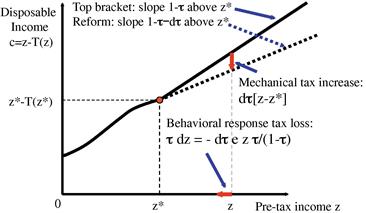
Figure 3 Optimal top tax rate derivation. The figure adapted from Diamond and Saez (2011), depicts the derivation of the optimal top tax rate ![]() by considering a small reform around the optimum which increases the top marginal tax rate
by considering a small reform around the optimum which increases the top marginal tax rate ![]() by
by ![]() above
above ![]() . A taxpayer with income
. A taxpayer with income ![]() mechanically pays
mechanically pays ![]() extra taxes but, by definition of the elasticity
extra taxes but, by definition of the elasticity ![]() of earnings with respect to the net-of-tax rate
of earnings with respect to the net-of-tax rate ![]() , also reduces his income by
, also reduces his income by ![]() leading to a loss in tax revenue equal to
leading to a loss in tax revenue equal to ![]() . Summing across all top bracket taxpayers and denoting by
. Summing across all top bracket taxpayers and denoting by ![]() the average income above
the average income above ![]() and
and ![]() , we obtain the revenue maximizing tax rate
, we obtain the revenue maximizing tax rate ![]() . This is the optimum tax rate when the government sets zero marginal welfare weights on top income earners.
. This is the optimum tax rate when the government sets zero marginal welfare weights on top income earners.
First, the optimal tax rate decreases with ![]() , the social marginal welfare weight on top bracket earners. In the limit case where society does not put any value on the marginal consumption of top earners, the formula simplifies to
, the social marginal welfare weight on top bracket earners. In the limit case where society does not put any value on the marginal consumption of top earners, the formula simplifies to ![]() which is the revenue maximizing top tax rate. A utilitarian social welfare criterion with marginal utility of consumption declining to zero, the most commonly used specification in optimal tax models following Mirrlees (1971), has the implication that
which is the revenue maximizing top tax rate. A utilitarian social welfare criterion with marginal utility of consumption declining to zero, the most commonly used specification in optimal tax models following Mirrlees (1971), has the implication that ![]() converges to zero when
converges to zero when ![]() grows to infinity.
grows to infinity.
Second, the optimal tax rate decreases with the elasticity ![]() as a higher elasticity leads to larger efficiency costs. Note that this elasticity is a mixture of substitution and income effects as an increase in the top tax rate generates both substitution and income effects.54 Importantly, for a given compensated elasticity, the presence of income effects increases the optimal top tax rate as raising the tax rate reduces disposable income and hence increases labor supply.
as a higher elasticity leads to larger efficiency costs. Note that this elasticity is a mixture of substitution and income effects as an increase in the top tax rate generates both substitution and income effects.54 Importantly, for a given compensated elasticity, the presence of income effects increases the optimal top tax rate as raising the tax rate reduces disposable income and hence increases labor supply.
Third, the optimal tax rate decreases with the parameter ![]() which measures the thinness of the top tail of the income distribution. Empirically,
which measures the thinness of the top tail of the income distribution. Empirically, ![]() is almost constant as
is almost constant as ![]() varies in the top tail of the earnings distribution. Figure 4 depicts
varies in the top tail of the earnings distribution. Figure 4 depicts ![]() (as a function of
(as a function of ![]() ) for the case of the US pre-tax income distribution and shows that it is extremely stable above
) for the case of the US pre-tax income distribution and shows that it is extremely stable above ![]() , approximately the top 1% threshold.55 This is due to the well-known fact—since at least Pareto (1896)—that the top tail is very closely approximated by a Pareto distribution.56
, approximately the top 1% threshold.55 This is due to the well-known fact—since at least Pareto (1896)—that the top tail is very closely approximated by a Pareto distribution.56
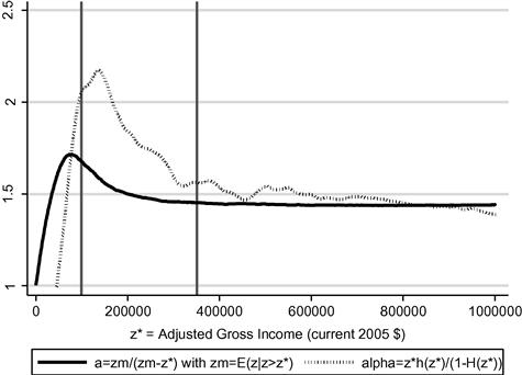
Figure 4 Empirical Pareto coefficients in the United States, 2005. The figure, from Diamond and Saez (2011), depicts in solid line the ratio ![]() with
with ![]() ranging from $0 to $1,000,000 annual income and
ranging from $0 to $1,000,000 annual income and ![]() the average income above
the average income above ![]() using US tax return micro data for 2005. Income is defined as Adjusted Gross Income reported on tax returns and is expressed in current 2005 dollars. Vertical lines depict the 90th percentile ($99,200) and 99th percentile ($350,500) nominal thresholds as of 2005. The ratio a is equal to one at
using US tax return micro data for 2005. Income is defined as Adjusted Gross Income reported on tax returns and is expressed in current 2005 dollars. Vertical lines depict the 90th percentile ($99,200) and 99th percentile ($350,500) nominal thresholds as of 2005. The ratio a is equal to one at ![]() , and is almost constant above the 99th percentile and slightly below 1.5, showing that the top of the distribution is extremely well approximated by a Pareto distribution for purposes of implementing the optimal top tax rate formula
, and is almost constant above the 99th percentile and slightly below 1.5, showing that the top of the distribution is extremely well approximated by a Pareto distribution for purposes of implementing the optimal top tax rate formula ![]() . Denoting by
. Denoting by ![]() the density and by
the density and by ![]() the cdf of the income distribution, the figure also displays in dotted line the ratio
the cdf of the income distribution, the figure also displays in dotted line the ratio ![]() which is also approximately constant, around 1.5, above the top percentile. A decreasing (or constant)
which is also approximately constant, around 1.5, above the top percentile. A decreasing (or constant) ![]() combined with a decreasing
combined with a decreasing ![]() and a constant
and a constant ![]() implies that the optimal marginal tax rate
implies that the optimal marginal tax rate ![]() increases with
increases with ![]() .
.
Fourth and related, the formula shows the limited relevance of the zero-top tax rate result. Formally, ![]() reaches 1 when
reaches 1 when ![]() reaches the level of income of the single highest income earner, in which case
reaches the level of income of the single highest income earner, in which case ![]() is infinite and indeed
is infinite and indeed ![]() , which is the famous zero-top rate result first demonstrated by Sadka (1976) and Seade (1977). However, notice that this result applies only to the very top income earner. Its lack of wider applicability can be verified empirically using distributional income tax statistics as we did in Figure 4 (see Saez, 2001 for an extensive analysis). Furthermore, under the reasonable assumption that the level of top earnings is not known in advance and where potential earnings are drawn randomly from an underlying Pareto distribution then, with the budget constraint satisfied in expectation, formula (7) remains the natural optimum tax rate (Diamond & Saez, 2011). This finding implies that the zero-top rate result and its corollary that marginal tax rates should decline at the top have no policy relevance.
, which is the famous zero-top rate result first demonstrated by Sadka (1976) and Seade (1977). However, notice that this result applies only to the very top income earner. Its lack of wider applicability can be verified empirically using distributional income tax statistics as we did in Figure 4 (see Saez, 2001 for an extensive analysis). Furthermore, under the reasonable assumption that the level of top earnings is not known in advance and where potential earnings are drawn randomly from an underlying Pareto distribution then, with the budget constraint satisfied in expectation, formula (7) remains the natural optimum tax rate (Diamond & Saez, 2011). This finding implies that the zero-top rate result and its corollary that marginal tax rates should decline at the top have no policy relevance.
Fifth, the optimal top tax rate formula is fairly general and applies equally to populations with heterogeneous preferences, discrete populations, or continuous populations. Although the optimal formula does not require the strong homogeneity assumptions of the Mirrlees (1971) problem, it is also the asymptotic limit of the optimal marginal tax rate of the fully nonlinear tax problem of Mirrlees (1971) as we shall see below.
5.1.2 Rent-Seeking Effects
Pay may not be equal to the marginal economic product for top income earners. In particular, executives can be overpaid if they are entrenched and can use their power to influence compensation committees. Indeed, a large literature in corporate finance has made those points (see for instance Bebchuk and Fried (2004) for an overview).57
There is relatively little work in optimal taxation that uses models where pay differs from marginal product.58 Here we adapt the very basic model of Piketty et al. (2011) to illustrate the key issues created by rent seeking effects. Rothschild and Scheuer (2011) consider a more elaborate model with rent-seeking and earnings heterogeneity with two sectors where rent-seeking activities prone to congestion are limited to a single sector.59
Let us assume that individual ![]() receives a fraction
receives a fraction ![]() of her actual product
of her actual product ![]() . Individual
. Individual ![]() can exert productive effort to increase
can exert productive effort to increase ![]() or bargaining effort to increase
or bargaining effort to increase ![]() . Both types of effort are costly to the individual. Hence, individual
. Both types of effort are costly to the individual. Hence, individual ![]() utility is given by
utility is given by
![]()
where ![]() is disposable after-tax income,
is disposable after-tax income, ![]() is the cost of producing output
is the cost of producing output ![]() as in the standard model, and
as in the standard model, and ![]() is the cost of bargaining to get a share
is the cost of bargaining to get a share ![]() of the product. Both
of the product. Both ![]() and
and ![]() are increasing and convex.
are increasing and convex.
Let ![]() be bargained earnings defined as the gap between received earnings
be bargained earnings defined as the gap between received earnings ![]() and actual product
and actual product ![]() . Note that the model allows both overpay (when
. Note that the model allows both overpay (when ![]() and hence
and hence ![]() ) and underpay (when
) and underpay (when ![]() and hence
and hence ![]() ). Let us denote by
). Let us denote by ![]() the average bargained earnings in the economy. In the aggregate, it must be the case that aggregate product must be equal to aggregate compensation. Hence, if
the average bargained earnings in the economy. In the aggregate, it must be the case that aggregate product must be equal to aggregate compensation. Hence, if ![]() , average overpay
, average overpay ![]() must come at the expense of somebody. Symmetrically, if
must come at the expense of somebody. Symmetrically, if ![]() , average underpay
, average underpay ![]() must benefit somebody. For simplicity, we assume that any gain made through bargaining comes at the expense of everybody else in the economy uniformly. Hence, individual incomes are all reduced by the same amount
must benefit somebody. For simplicity, we assume that any gain made through bargaining comes at the expense of everybody else in the economy uniformly. Hence, individual incomes are all reduced by the same amount ![]() (or increased by −
(or increased by −![]() if
if ![]() ).60
).60
Because the government uses a nonlinear income tax schedule, it can adjust the demogrant intercept ![]() to fully offset
to fully offset ![]() . Effectively, the government can always tax (or subsidize)
. Effectively, the government can always tax (or subsidize) ![]() at 100% before applying its nonlinear income tax. Hence, we can assume without loss of generality that the government absorbs one-for-one any change in
at 100% before applying its nonlinear income tax. Hence, we can assume without loss of generality that the government absorbs one-for-one any change in ![]() . Therefore, we can simply define earnings as
. Therefore, we can simply define earnings as ![]() and assume that those earnings are taxed nonlinearly.
and assume that those earnings are taxed nonlinearly.
Individual ![]() chooses
chooses ![]() and
and ![]() to maximize:
to maximize:
![]()
which leads to the first order conditions
![]()
where ![]() is the marginal tax rate. This naturally defines
is the marginal tax rate. This naturally defines ![]() as increasing functions of the net-of-tax rate
as increasing functions of the net-of-tax rate ![]() . Hence
. Hence ![]() and
and ![]() are also functions of
are also functions of ![]() .
.
Let us consider as in the previous section the optimal top tax rate ![]() above income level
above income level ![]() . We assume again that there is a fraction
. We assume again that there is a fraction ![]() of top bracket taxpayers. Let us denote by
of top bracket taxpayers. Let us denote by ![]() average reported income, productive earnings, and bargained earnings across all taxpayers in the top bracket. We can then define the real labor supply elasticity
average reported income, productive earnings, and bargained earnings across all taxpayers in the top bracket. We can then define the real labor supply elasticity ![]() and the total compensation elasticity
and the total compensation elasticity ![]() as:
as:
![]()
We define ![]() as the fraction of the marginal behavioral response due to bargaining and let
as the fraction of the marginal behavioral response due to bargaining and let ![]() be the bargaining elasticity component:
be the bargaining elasticity component:
![]()
This definition immediately implies that ![]() . By construction,
. By construction, ![]() . Importantly,
. Importantly, ![]() (and hence
(and hence ![]() ) can be either positive or negative but it is always positive if individuals are overpaid (i.e., if
) can be either positive or negative but it is always positive if individuals are overpaid (i.e., if ![]() ). If individuals are underpaid (i.e.,
). If individuals are underpaid (i.e., ![]() ) then
) then ![]() (and hence
(and hence ![]() ) may be negative.
) may be negative.
For simplicity, let us assume that bargaining effects are limited to individuals in the top bracket. As there is a fraction ![]() of top brackets individuals, we hence have
of top brackets individuals, we hence have ![]() . We assume that the government wants to maximize tax revenue collected from top bracket earners, taking into account bargaining effects:
. We assume that the government wants to maximize tax revenue collected from top bracket earners, taking into account bargaining effects:
![]()
The second term ![]() arises because we assume that average underpay
arises because we assume that average underpay ![]()
due to rent-seeking at the top is fully absorbed by the government budget as discussed above.
In this model, the top tax rate maximizing tax revenue satisfies the first order condition
![]()
The last term reflects the rent-seeking externality. Any decrease in top incomes due to a reduction in ![]() creates a positive externality on all individuals, which can be recouped by the government by adjusting the demogrant. The optimal top tax rate can then be rewritten as follows:
creates a positive externality on all individuals, which can be recouped by the government by adjusting the demogrant. The optimal top tax rate can then be rewritten as follows:
![]() (8)
(8)
![]() decreases with the total
decreases with the total ![]() (keeping the bargaining component
(keeping the bargaining component ![]() constant) and increases with
constant) and increases with ![]() (keeping
(keeping ![]() constant). It also decreases with the real elasticity
constant). It also decreases with the real elasticity ![]() (keeping
(keeping ![]() and
and ![]() constant) and increases with the level of overpayment
constant) and increases with the level of overpayment ![]() (keeping
(keeping ![]() and
and ![]() constant). If
constant). If ![]() then
then ![]() . Two scenarios are theoretically possible.
. Two scenarios are theoretically possible.
Trickle-Up. In the case where top earners are overpaid relative to their productivity (![]() ), then
), then ![]() and hence
and hence ![]() and the optimal top tax rate is higher than in the standard model (i.e.,
and the optimal top tax rate is higher than in the standard model (i.e., ![]() ). This corresponds to a “trickle-up” situation where a tax cut on upper incomes shifts economic resources away from the bottom and toward the top. Those effects can have a large quantitative impact on optimal top tax rates. In the extreme case where all behavioral responses at the top are due to rent-seeking effects (
). This corresponds to a “trickle-up” situation where a tax cut on upper incomes shifts economic resources away from the bottom and toward the top. Those effects can have a large quantitative impact on optimal top tax rates. In the extreme case where all behavioral responses at the top are due to rent-seeking effects (![]() and
and ![]() ) then
) then ![]() .
.
Trickle-Down. In the case where top earners are underpaid relative to their productivity (![]() ) it is possible to have
) it is possible to have ![]() and hence
and hence ![]() , in which case the optimal top tax rate is lower than in the standard model (i.e.,
, in which case the optimal top tax rate is lower than in the standard model (i.e., ![]() ). This corresponds to a “trickle-down” situation where a tax cut on upper incomes also shifts economic resources toward the bottom, as upper incomes are underpaid and hence work in part for the benefit of lower incomes.
). This corresponds to a “trickle-down” situation where a tax cut on upper incomes also shifts economic resources toward the bottom, as upper incomes are underpaid and hence work in part for the benefit of lower incomes.
Implementing formula (8) requires knowing not only how compensation responds to tax changes but also how real economic product responds to tax changes, which is considerably more difficult than estimating the standard taxable income elasticity ![]() (see Piketty et al., 2011 for such an attempt). The issue of whether top earners deserve their incomes or are rent-seekers certainly looms large in the debate on top income taxation. Yet little empirical evidence can bear on the issue. This illustrates the limits of the theory of optimal taxation. Realistic departures from the standard economic model might be difficult to measure and yet can affect optimal tax rates in substantial ways.61
(see Piketty et al., 2011 for such an attempt). The issue of whether top earners deserve their incomes or are rent-seekers certainly looms large in the debate on top income taxation. Yet little empirical evidence can bear on the issue. This illustrates the limits of the theory of optimal taxation. Realistic departures from the standard economic model might be difficult to measure and yet can affect optimal tax rates in substantial ways.61
Finally, note that the model with rent-seeking is also related to the derivation of the optimal tax rates in the presence of externalities due to charitable giving responses (see e.g., Saez, 2004a) or the presence of transfers across agents (Chetty, 2009b).
5.1.3 International Migration
Taxes and transfers might affect migration in or out of the country. For example, high top tax rates might induce highly skilled workers to emigrate to low top tax rate countries.62
We consider a simplified version of the migration model of Mirrlees (1982) in order to obtain a simple formula.63
Let us assume that the only behavioral response to taxes is migration so that individual earnings ![]() conditional on residence are fixed. Let us denote by
conditional on residence are fixed. Let us denote by ![]() the number of resident individuals earning
the number of resident individuals earning ![]() when disposable domestic income is
when disposable domestic income is ![]() . With the income tax, we have
. With the income tax, we have ![]() . We assume that
. We assume that ![]() increases with
increases with ![]() due to migration responses.
due to migration responses.
We can consider a small reform which increases taxes by ![]() for those earning
for those earning ![]() . The mechanical effect net of welfare is
. The mechanical effect net of welfare is ![]() where
where ![]() is the social marginal welfare weight on individuals with earnings
is the social marginal welfare weight on individuals with earnings ![]() . The net fiscal cost of somebody earning
. The net fiscal cost of somebody earning ![]() emigrating is
emigrating is ![]() . We can define an elasticity of migration with respect to disposable income
. We can define an elasticity of migration with respect to disposable income ![]() . Hence the fiscal cost is
. Hence the fiscal cost is ![]() . Marginal emigrants are indifferent between emigrating or staying and hence the welfare cost is second order in this case as well. At the optimum, we have
. Marginal emigrants are indifferent between emigrating or staying and hence the welfare cost is second order in this case as well. At the optimum, we have ![]() , which implies:
, which implies:
![]() (9)
(9)
In the EU context, the most interesting application of the tax induced migration model is at the high income end. Indeed, there have been heated discussions of brain drain issues across EU countries due to differential tax rates at the top across countries. If we assume that high incomes respond both along the intensive margin as in Section 5.1.1 with elasticity ![]() , and along the migration margin with elasticity
, and along the migration margin with elasticity ![]() , then, it is possible to show that the optimal top rate maximizing tax revenue becomes (see Brewer, Shephard, & Saez, 2010):
, then, it is possible to show that the optimal top rate maximizing tax revenue becomes (see Brewer, Shephard, & Saez, 2010):
![]() (10)
(10)
For example if ![]() , the optimal tax rate with no migration is
, the optimal tax rate with no migration is ![]() . If there is migration with elasticity
. If there is migration with elasticity ![]() , then the optimal tax rate decreases to
, then the optimal tax rate decreases to ![]() . Thus, large migration elasticities could indeed decrease significantly the ability of European countries to tax high incomes.
. Thus, large migration elasticities could indeed decrease significantly the ability of European countries to tax high incomes.
Two important additional points should be made. First, the size of the migration elasticity ![]() depends not only on individual preferences but also on the size of the jurisdiction. Small jurisdictions—such as a town—typically have large elasticities as individuals can relocate outside the jurisdiction at low costs, for example without having to change jobs, etc. (see the chapter in this volume by Glaeser on urban public finance for a detailed discussion). The elasticity becomes infinite in the case of very small jurisdictions. Conversely, very large jurisdictions—such as a large country—have lower elasticities as it is costly to relocate. In the limit case of the full world, the migration elasticity is naturally zero. Therefore and as is well known, it is harder for small jurisdictions to implement redistributive taxation and indeed most redistributive tax and transfer programs tend to be carried out at the country level rather than the regional or city level.
depends not only on individual preferences but also on the size of the jurisdiction. Small jurisdictions—such as a town—typically have large elasticities as individuals can relocate outside the jurisdiction at low costs, for example without having to change jobs, etc. (see the chapter in this volume by Glaeser on urban public finance for a detailed discussion). The elasticity becomes infinite in the case of very small jurisdictions. Conversely, very large jurisdictions—such as a large country—have lower elasticities as it is costly to relocate. In the limit case of the full world, the migration elasticity is naturally zero. Therefore and as is well known, it is harder for small jurisdictions to implement redistributive taxation and indeed most redistributive tax and transfer programs tend to be carried out at the country level rather than the regional or city level.
Second and related, a single jurisdiction does not recognize the external cost it might impose on others by cutting its top tax rate. In that case, fiscal coordination across jurisdictions (e.g., European countries) could be mutually beneficial to internalize the externality. With complete fiscal coordination, the migration elasticity again becomes irrelevant for optimal tax policy (see the chapter by Keen and Konrad in this volume for an complete treatment of tax competition issues). When making policy recommendations, economists should try to be as clear as possible as to whether they are concerned with a single country optimum or with a global welfare perspective.64