
5.1.4 Empirical Evidence on Top Incomes and Top Tax Rates
Micro-Level Tax Reform Studies. A very large literature has used tax reforms and micro-level tax return data to identify the elasticity of reported incomes with respect to the net-of-tax marginal rate. Those studies typically compare changes in pre-tax incomes of groups affected by a tax reform to changes in pre-tax incomes of groups unaffected by the reform. Hence, such tax reform-based analysis can only estimate short-term responses (typically 1–5 years) to tax changes. This literature, surveyed in Saez, Slemrod, and Giertz (2012), obtains three key conclusions that we briefly summarize here. First, there is substantial heterogeneity in the estimates: Many studies finding relatively small elasticity estimates (below 0.25), but some have found that tax reform episodes do generate large short-term behavioral responses, which imply large elasticities, particularly at the top of the income distribution. Second however, all the cases with large behavioral responses are due to tax avoidance such as retiming or income shifting. To our knowledge, none of the empirical tax reform studies to date have shown large responses due to changes in real economic behavior such as labor supply or business creation.65 Furthermore, “anatomy analysis” shows that the large tax avoidance responses obtained are always the consequence of poorly designed tax systems offering arbitrage opportunities66 or income retiming opportunities in anticipation of or just after-tax reforms.67 When the tax system offers few tax avoidance opportunities, short-term responses to changes in tax rates are fairly modest with elasticities typically below 0.25.68 Therefore, the results from this literature fit well with the tax avoidance model presented above with fairly small real elasticities and potentially large avoidance elasticities that can be sharply reduced through better tax design.
International Mobility. Mobility responses to taxation often loom larger in the policy debate on tax progressivity than traditional within country labor supply responses.69 A large literature has shown that capital income mobility is a substantial concern (see e.g. the chapter by Keen and Konrad in this volume). However, there is much less empirical work on the effect of taxation on the spatial mobility of individuals, especially among high-skilled workers. A small literature has considered the mobility of people across local jurisdictions within countries.70 While mobility costs within a country may be small, within country variations in taxes also tend to be modest. Therefore, it is difficult to extrapolate from those studies to international migration where both tax differentials and mobility costs are much higher. There is very little empirical work on the effect of taxation on international mobility partly due to lack of micro data with citizenship information and challenges in identifying causal tax effects on migration. In recent decades however, many countries, particularly in Europe, have introduced preferential tax rates for specific groups of foreign workers, and often highly paid foreign workers (see OECD, 2011c, chap. 4, Table 4.1, p. 138 for a summary of all such existing schemes). Such preferential tax schemes offer a promising route to identify tax induced mobility effects, recently exploited in two studies.
Kleven, Landais, and Saez (2013) study the tax induced mobility of professional football players in Europe and find substantial mobility elasticities. The mobility elasticity of the number of domestic players with respect to the domestic net-of-tax rate is relatively small, around .15. However, the mobility elasticity of the number of foreign players with respect to the net-of-tax rate that applies to foreign players is much larger, around 1. This difference is due to the fact that most players still play in their home country. Kleven et al. (in press) confirm that this latter result applies to the broader market of highly skilled foreign workers and not only football players. They show, in the case study of Denmark, that the preferential tax scheme for highly paid foreigners introduced in 1991 doubled the number of high earning foreigners in Denmark. This translates again into an elasticity of the number of foreign workers with respect to the net-of-tax rate above one.
Those results imply that, from a single country’s perspective, as the number of foreigners at the top is still relatively small, the migration elasticity ![]() of all top earners with respect to a single net-of-tax top rate is still relatively small, likely below .25 for most countries. This is the relevant elasticity to use in formula (10). Hence, the top income tax rate calculation is unlikely to be drastically affected by migration effects. However, this elasticity is likely to grow overtime as labor markets become better integrated and the fraction of foreign workers grows. Nevertheless, because the elasticity of the number of foreign workers with respect to the net-of-tax rate applying to foreign workers is so large, it is indeed advantageous from a single country perspective to offer such preferential tax schemes. This could explain why such schemes have proliferated in Europe in recent years. Such schemes are typical beggar-thy-neighbor policies which reduce the collective ability of countries to tax top earners. Hence, regulating such schemes at a supranational level (for example at the European Union level for European countries) is likely to become a key element in tax coordination policy debates.
of all top earners with respect to a single net-of-tax top rate is still relatively small, likely below .25 for most countries. This is the relevant elasticity to use in formula (10). Hence, the top income tax rate calculation is unlikely to be drastically affected by migration effects. However, this elasticity is likely to grow overtime as labor markets become better integrated and the fraction of foreign workers grows. Nevertheless, because the elasticity of the number of foreign workers with respect to the net-of-tax rate applying to foreign workers is so large, it is indeed advantageous from a single country perspective to offer such preferential tax schemes. This could explain why such schemes have proliferated in Europe in recent years. Such schemes are typical beggar-thy-neighbor policies which reduce the collective ability of countries to tax top earners. Hence, regulating such schemes at a supranational level (for example at the European Union level for European countries) is likely to become a key element in tax coordination policy debates.
Cross Country and Time Series Evidence. The simplest way to obtain evidence on the long-term behavioral responses of top incomes to tax rates is to use long time series analysis within a country or across countries. Data on top incomes overtime and across countries have been compiled by a number of recent studies (see Atkinson et al., 2011 for a survey) and gathered in the World Top Incomes Database (Alvaredo, Atkinson, Piketty & Saez 2011. A few recent studies have analyzed the link between top income shares and top tax rates (Atkinson & Leigh, 2010; Roine, Vlachos, & Waldenstrom, 2009; Piketty et al., 2011).
There is a strong negative correlation between top tax rates and top income shares, such as the fraction of total income going to the top 1% of the distribution. This long-run correlation is present overtime within countries as well as across countries. As an important caveat, the correlation between top tax rates and top income shares may not be causal as other policies potentially affecting top income shares, such as financial or industrial regulation or policies affecting Unions, may be correlated with top tax rate policy, creating an omitted variable bias. Alternatively and in reverse causality, higher top income shares may increase the political influence of top earners leading to lower top tax rates.71
Panel A in Figure 5 illustrates the cross-country evidence. It plots the change in top income shares from 1960–1964 to 2004–2009 (on the y-axis) against the change in the top marginal tax rate (on the x-axis) for 18 OECD countries. The figure shows a very clear and strong correlation between the cut in top tax rates and the increase in the top 1% income share with interesting heterogeneity. Countries such as France, Germany, Spain, Denmark, or Switzerland which did not experience any significant top rate tax cut did not experience large changes in top 1% income shares. Among the countries which experienced significant top rate cuts, some experience a large increase in top income shares (all five English speaking countries but also Norway and Finland) while others experience only modest increases in top income shares (Japan, Italy, Sweden, Portugal, and the Netherlands). Interestingly, no country experiences a significant increase in top income shares without implementing significant top rate tax cuts. Overall, the elasticity implied by this correlation is large, above 0.5. However, this evidence cannot tell whether the elasticity is due to real effects, tax evasion, or rent-seeking effects.

Figure 5 Top marginal tax rates and top incomes shares. This figure is from Piketty, Saez, and Stantcheva (2011). Panel A depicts the change in pre-tax top income shares against the change in pre-tax top income tax rate from 1960–1964 to 2005–2009 based on data for 18 OECD countries (exact years depend on availability of top income share data in the World Top Incomes Database (Alvaredo et al., 2011)). Panel B depicts the pre-tax top 1% US income shares including realized capital gains in full diamonds and excluding realized capital gains in empty diamonds from 1913 to 2010. Computations are based on family market cash income. Income excludes government transfers and is before individual taxes (source is Piketty and Saez (2003), series updated to 2010). Panel B also depicts the top marginal tax rate on ordinary income and on realized long-term capital gains.
Panel B in Figure 5 illustrates the time series evidence for the case of the United States. It depicts the top 1% income shares including realized capital gains (pictured with full diamonds) and excluding realized capital gains (the empty diamonds) since 1913, which marks the introduction of the US federal income tax. Both top income shares, whether including or excluding realized capital gains, display an overall U-shape over the century. Panel A also displays (on the right y-axis) the federal individual income top marginal tax rate for ordinary income (dashed line), and for long-term realized capital gains (dotted line). Two important lessons emerge from this panel. Considering first the top income share excluding realized capital gains which corresponds roughly to income taxed according to the regular progressive schedule, there is a clear negative overall correlation between the top 1% income share and the top marginal tax rate, showing again that the elasticity of reported income with respect to the net-of-tax rate is large in the long run. Second, the correlation between the top 1% income share and the top tax rate also holds for the series including capital gains. Realized capital gains have been traditionally tax favored (as illustrated by the gap between the top tax rate and the tax rate on realized capital gains in the figure) and have constituted the main channel for tax avoidance of upper incomes.72 This suggests that, in contrast to short-run tax reform analysis, income shifting responses cannot be the main channel creating the long-run correlation between top income shares and top tax rates.73
If the long-term correlation between top income shares and top tax rates is not driven by tax avoidance, the key question is whether it is driven by real supply side responses or whether it reflects rent-seeking effects whereby top earners can gain at the expense of others when top rates are low. In principle, the two types of behavioral responses can be distinguished by looking at economic growth as supply-side responses affect economic growth while rent-seeking responses do not. Piketty et al. (2011) analyze cross-country time series for OECD countries since 1960 and do not find any evidence that cuts in top tax rates stimulate growth. This suggests that rent-seeking effects likely play a role in the correlation between top tax rates and top incomes, and therefore that optimal top tax rates might be substantially larger than what it commonly assumed (say, above 80% rather than 50–60%). In our view, this is the right model to account for the quasi-confiscatory top tax rates during large parts of the 20th century (particularly in the US and in the UK; see Figure 1 above). Needless to say, more compelling empirical identification would be very useful to cast further light on this key issue for the optimal taxation of top earners.74
5.2 Optimal Nonlinear Schedule
5.2.1 Continuous Model of Mirrlees
It is possible to obtain the formula for the optimal marginal tax rate ![]() at income level
at income level ![]() for the fully general nonlinear income tax using a similar variational method as the one used to derive the top income tax rate. To simplify the exposition, we consider the case with no income effects, where labor supply depends solely on the net-of-tax rate
for the fully general nonlinear income tax using a similar variational method as the one used to derive the top income tax rate. To simplify the exposition, we consider the case with no income effects, where labor supply depends solely on the net-of-tax rate ![]() .75 We present in the text a graphical proof adapted from Saez (2001) and Diamond and Saez (2011) and we relegate to the appendix the formal presentation and derivation in the standard Mirrlees model with no income effects (as in the analysis of Diamond, 1998).
.75 We present in the text a graphical proof adapted from Saez (2001) and Diamond and Saez (2011) and we relegate to the appendix the formal presentation and derivation in the standard Mirrlees model with no income effects (as in the analysis of Diamond, 1998).
Figure 6 depicts the optimal marginal tax rate derivation at income level ![]() . Again, the horizontal axis in Figure 6 shows pre-tax income, while the vertical axis shows disposable income. Consider a situation in which the marginal tax rate is increased by
. Again, the horizontal axis in Figure 6 shows pre-tax income, while the vertical axis shows disposable income. Consider a situation in which the marginal tax rate is increased by ![]() in the small band from
in the small band from ![]() to
to ![]() , but left unchanged anywhere else. The tax reform has three effects.
, but left unchanged anywhere else. The tax reform has three effects.
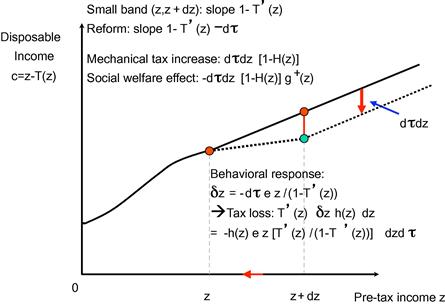
Figure 6 Derivation of the optimal marginal tax rate at income level ![]() . The figure, adapted from Diamond and Saez (2011), depicts the optimal marginal tax rate derivation at income level
. The figure, adapted from Diamond and Saez (2011), depicts the optimal marginal tax rate derivation at income level ![]() by considering a small reform around the optimum, whereby the marginal tax rate in the small band
by considering a small reform around the optimum, whereby the marginal tax rate in the small band ![]() is increased by
is increased by ![]() . This reform mechanically increases taxes by
. This reform mechanically increases taxes by ![]() for all taxpayers above the small band, leading to a mechanical tax increase
for all taxpayers above the small band, leading to a mechanical tax increase ![]() and a social welfare cost of
and a social welfare cost of ![]() . Assuming away income effects, the only behavioral response is a substitution effect in the small band: The
. Assuming away income effects, the only behavioral response is a substitution effect in the small band: The ![]() taxpayers in the band reduce their income by
taxpayers in the band reduce their income by ![]() leading to a tax loss equal to
leading to a tax loss equal to ![]() . At the optimum, the three effects cancel out leading to the optimal tax formula
. At the optimum, the three effects cancel out leading to the optimal tax formula ![]() , or equivalently
, or equivalently ![]() after introducing
after introducing ![]() .
.
First, the mechanical tax increase, leaving aside behavioral responses, will be the gap between the solid and dashed lines, shown by the vertical arrow equal to ![]() . The total mechanical tax increase is
. The total mechanical tax increase is ![]() as there are
as there are ![]() individuals above
individuals above ![]() .
.
Second, this tax increase creates a social welfare cost of ![]() where
where ![]() is defined as the average (unweighted) social marginal welfare weight for individuals with income above
is defined as the average (unweighted) social marginal welfare weight for individuals with income above ![]() .
.
Third, there is a behavioral response to the tax change. Those in the income range from ![]() to
to ![]() have a behavioral response to the higher marginal tax rate, shown by the horizontal line pointing left. Assuming away income effects, this is the only behavioral response; those with income levels above
have a behavioral response to the higher marginal tax rate, shown by the horizontal line pointing left. Assuming away income effects, this is the only behavioral response; those with income levels above ![]() face no change in marginal tax rates and hence have no behavioral response. A taxpayer in the small band reduces her income by
face no change in marginal tax rates and hence have no behavioral response. A taxpayer in the small band reduces her income by ![]() where
where ![]() is the elasticity of earnings
is the elasticity of earnings ![]() with respect to the net-of-tax rate
with respect to the net-of-tax rate ![]() . As there are
. As there are ![]() taxpayers in the band, those behavioral responses lead to a tax loss equal to
taxpayers in the band, those behavioral responses lead to a tax loss equal to ![]() .76
.76
At the optimum, the three effects should cancel out so that ![]() . Define the local Pareto parameter as
. Define the local Pareto parameter as ![]() .77 This leads to the following optimal tax formula
.77 This leads to the following optimal tax formula
![]() (11)
(11)
Formula (11) has essentially the same form as (7). Five further points are worth noting.
First, the simple graphical proof shows that the formula does not depend on the strong homogeneity assumptions of the standard Mirrlees model where individuals differ solely through a skill parameter. This implies that the formula actually carries over to heterogeneous populations as is the case of the basic linear tax rate formula (3).78
Second, the optimal tax rate naturally decreases with ![]() , the average social marginal welfare weight above
, the average social marginal welfare weight above ![]() . Under standard assumptions where social marginal welfare weights decrease with income,
. Under standard assumptions where social marginal welfare weights decrease with income, ![]() is decreasing in
is decreasing in ![]() . With no income effects, the average social marginal welfare weight is equal to one (see Section 3.1) so that
. With no income effects, the average social marginal welfare weight is equal to one (see Section 3.1) so that ![]() and
and ![]() for
for ![]() . This immediately implies that
. This immediately implies that ![]() for any
for any ![]() , one of the few general results coming out of the Mirrlees model and first demonstrated by Mirrlees (1971) and Seade (1982).79 A decreasing
, one of the few general results coming out of the Mirrlees model and first demonstrated by Mirrlees (1971) and Seade (1982).79 A decreasing ![]() tends to make the tax system more progressive. Note that the extreme Rawlsian case has
tends to make the tax system more progressive. Note that the extreme Rawlsian case has ![]() for all
for all ![]() except at
except at ![]() (assuming realistically that the most disadvantaged are those with no earnings). In that case, the formula simplifies to
(assuming realistically that the most disadvantaged are those with no earnings). In that case, the formula simplifies to ![]() and the optimal tax system maximizes tax revenue raised to make the lump sum demogrant
and the optimal tax system maximizes tax revenue raised to make the lump sum demogrant ![]() as large as possible.
as large as possible.
Third, the optimal tax rate decreases with the elasticity ![]() at income level
at income level ![]() as a higher elasticity leads to larger efficiency costs in the small band
as a higher elasticity leads to larger efficiency costs in the small band ![]() . Note that this elasticity remains a pure substitution elasticity even in the presence of income effects.80
. Note that this elasticity remains a pure substitution elasticity even in the presence of income effects.80
Fourth, the optimal tax rate decreases with the local Pareto parameter ![]() which reflects the ratio of the total income of those affected by the marginal tax rate at
which reflects the ratio of the total income of those affected by the marginal tax rate at ![]() relative to the number of people at higher income levels. The intuition for this follows the derivation from Figure 6. Increasing
relative to the number of people at higher income levels. The intuition for this follows the derivation from Figure 6. Increasing ![]() creates efficiency costs proportional to the number of people at income level
creates efficiency costs proportional to the number of people at income level ![]() times the income level
times the income level ![]() while it raises more taxes (with no distortion) from everybody above
while it raises more taxes (with no distortion) from everybody above ![]() . As shown on Figure 4 for the US case, empirically
. As shown on Figure 4 for the US case, empirically ![]() first increases and then decreases before being approximately constant in the top tail. Hence, when
first increases and then decreases before being approximately constant in the top tail. Hence, when ![]() is large, formula (11) converges to the optimal top rate formula (7) that we derived earlier.
is large, formula (11) converges to the optimal top rate formula (7) that we derived earlier.
Fifth, suppose the government has no taste for redistribution and wants to raise an exogenous amount of revenue while minimizing efficiency costs. If lump sum taxes are realistically ruled out because those with no earnings could not possibly pay them, then the optimal tax system is still given by ( 11) with constant social marginal welfare weights and hence constant ![]() set to exactly raise the needed amount of exogenous revenue (Saez, 1999, chap. 3).
set to exactly raise the needed amount of exogenous revenue (Saez, 1999, chap. 3).
Increasing Marginal Tax Rates at the Top. With an elasticity ![]() constant across income groups, as
constant across income groups, as ![]() decreases with
decreases with ![]() and
and ![]() also decreases with
also decreases with ![]() in the upper part of the distribution (approximately the top 5% in the US case, see Figure 4), formula (11) implies that the optimal marginal tax rate should increase with
in the upper part of the distribution (approximately the top 5% in the US case, see Figure 4), formula (11) implies that the optimal marginal tax rate should increase with ![]() at the upper end, i.e., the income tax should be progressive at the top. Diamond (1998) provides formal theoretical results in the Mirrlees model with no income effects.
at the upper end, i.e., the income tax should be progressive at the top. Diamond (1998) provides formal theoretical results in the Mirrlees model with no income effects.
Numerical Simulations. For low ![]() decreases but
decreases but ![]() increases. Numerical simulations calibrated using the actual US earnings distribution presented in Saez (2001) show that the
increases. Numerical simulations calibrated using the actual US earnings distribution presented in Saez (2001) show that the ![]() effect dominates at the bottom so that the marginal tax rate is high and decreasing for low
effect dominates at the bottom so that the marginal tax rate is high and decreasing for low ![]() . We come back to this important issue when we discuss the optimal profile of transfers below. Therefore, assuming that the elasticity is constant with
. We come back to this important issue when we discuss the optimal profile of transfers below. Therefore, assuming that the elasticity is constant with ![]() , the optimal marginal tax rate in the Mirrlees model is U-shaped with income, first decreasing with income and then increasing with income before converging to its limit value given by formula (7).
, the optimal marginal tax rate in the Mirrlees model is U-shaped with income, first decreasing with income and then increasing with income before converging to its limit value given by formula (7).
5.2.2 Discrete Models
Stiglitz (1982) developed the 2 skill-type discrete version of the Mirrlees (1971) model where individuals can have either a low or a high wage rate. This discrete model has been used widely in the subsequent literature because it has long been perceived as more tractable than the continuous model of Mirrlees. However, the discrete model is perhaps deceiving when it comes to understanding optimal tax progressivity. Indeed, the zero top marginal tax rate result implies that the marginal tax rate on the highest skill is zero and hence lower than the marginal tax rate on the lowest skill, suggesting that the marginal tax rate should decrease with earnings. Furthermore, it is impossible to express optimal tax formulas in the Stiglitz (1982) model in terms of estimable statistics and hence to quantitatively calibrate the model.
More recently, Piketty (1997) introduced and Saez (2002a) further developed an alternative form of discrete Mirrlees model with a finite number of possible earnings levels ![]() (corresponding for example to different possible jobs) but a continuum of individual types so that the fraction of individuals at each earnings level is a smooth function of the tax system. This model generates formulas close to the continuum case, and can also be easily extended to incorporate extensive labor supply responses, as we shall see.
(corresponding for example to different possible jobs) but a continuum of individual types so that the fraction of individuals at each earnings level is a smooth function of the tax system. This model generates formulas close to the continuum case, and can also be easily extended to incorporate extensive labor supply responses, as we shall see.
Formally, individual ![]() has a utility function
has a utility function ![]() defined on after-tax income
defined on after-tax income ![]() and job choice
and job choice ![]() . Each individual chooses
. Each individual chooses ![]() to maximize
to maximize ![]() where
where ![]() is the after-tax reward in occupation
is the after-tax reward in occupation ![]() . For a given tax and transfer schedule
. For a given tax and transfer schedule ![]() , a fraction
, a fraction ![]() of individuals choose occupation
of individuals choose occupation ![]() . It is assumed that the tastes for work embodied in the individual utilities are smoothly distributed so that the aggregate functions
. It is assumed that the tastes for work embodied in the individual utilities are smoothly distributed so that the aggregate functions ![]() are differentiable. Denoting by
are differentiable. Denoting by ![]() the occupational choice of individual
the occupational choice of individual ![]() , the government chooses
, the government chooses ![]() so as to maximize welfare
so as to maximize welfare
![]()
Even though the population is potentially very heterogeneous, as possible work outcomes are in finite number, the maximization problem is a simple finite dimensional maximization problem. The first order condition with respect to ![]() is
is
 (12)
(12)
Hence, ![]() is the average social marginal welfare weight among individuals in occupation
is the average social marginal welfare weight among individuals in occupation ![]() .81
.81
This model allows for any type of behavioral responses. Two special cases are of particular interest: pure intensive responses as in the standard Mirrlees (1971) model and pure extensive responses. We consider in this section the intensive model case and defer to Section 5.3.2 the extensive model case.
The intensive model. The intensive model with no income effects (first developed by Piketty, 1997) can be obtained by assuming that the population is partitioned into ![]() groups. An individual in group
groups. An individual in group ![]() can only work in two adjacent occupations
can only work in two adjacent occupations ![]() and
and ![]() . For example, with no effort the individual can hold job
. For example, with no effort the individual can hold job ![]() and with some effort the individual can obtain job
and with some effort the individual can obtain job ![]() .82 This implies that the function
.82 This implies that the function ![]() depends only on
depends only on ![]() , and
, and ![]() . Assuming no income effects, with a slight abuse of notation,
. Assuming no income effects, with a slight abuse of notation, ![]() can be expressed as
can be expressed as ![]() . In that context, we can denote by
. In that context, we can denote by ![]() the marginal tax rate between earnings levels
the marginal tax rate between earnings levels ![]() and
and ![]() and by
and by ![]() the elasticity of the fraction of individuals in occupation
the elasticity of the fraction of individuals in occupation ![]() with respect to the net-of-tax rate
with respect to the net-of-tax rate ![]() . The optimal tax formula (12) can be rearranged as:
. The optimal tax formula (12) can be rearranged as:
![]() (13)
(13)
The proof is presented in Saez (2002a). Note that the form of the optimal formula is actually very close the continuum case where the marginal tax rate from Eq. (11) can also be written as: ![]() .
.
5.3 Optimal Profile of Transfers
5.3.1 Intensive Margin Responses
It is possible to obtain a formula for the optimal phase-out rate of the demogrant in the optimal income tax model of Mirrlees (1971) where labor supply responds only through the intensive margin.
Recall first that when the minimum income ![]() is positive, the optimal marginal tax rate at the very bottom is zero (this result was first proved by Seade, 1977). This can be seen from formula (11) as
is positive, the optimal marginal tax rate at the very bottom is zero (this result was first proved by Seade, 1977). This can be seen from formula (11) as ![]() .83
.83
However, the empirically relevant case is ![]() with a non-zero fraction
with a non-zero fraction ![]() of the population not working and earning zero. In that case, the optimal phase-out rate
of the population not working and earning zero. In that case, the optimal phase-out rate ![]()
at the bottom can be written as:
![]() (14)
(14)
where ![]() is the average social marginal welfare weight on zero earners and
is the average social marginal welfare weight on zero earners and ![]() is the elasticity of the fraction non-working
is the elasticity of the fraction non-working ![]() with respect to the bottom net-of-tax rate
with respect to the bottom net-of-tax rate ![]() with a minus sign so that
with a minus sign so that ![]() .84 This formula is proved by Saez (2002a) in the discrete model presented above.85
.84 This formula is proved by Saez (2002a) in the discrete model presented above.85
The formula also applies in the standard Mirrlees model although it does not seem to have been ever noticed and formally presented. We present the proof in the standard Mirrlees model in the appendix. In the text, we present a simple graphical proof adapted from Diamond and Saez (2011) using the discrete model with intensive margin responses presented above.
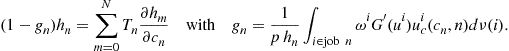
As illustrated on Figure 7, suppose that low ability individuals can choose either to work and earn ![]() or not work and earn zero (
or not work and earn zero (![]() ). The government offers a transfer
). The government offers a transfer ![]() to those not working phased-out at rate
to those not working phased-out at rate ![]() so that those working receive on net
so that those working receive on net ![]() . In words, non-workers keep a fraction
. In words, non-workers keep a fraction ![]() of their earnings should they work and earn
of their earnings should they work and earn ![]() . Therefore, increasing
. Therefore, increasing ![]() discourages some low income workers from working. Suppose now that the government increases both the
discourages some low income workers from working. Suppose now that the government increases both the ![]() by
by ![]() and the phase-out rate by
and the phase-out rate by ![]() leaving the tax schedule unchanged for those with income equal to or above
leaving the tax schedule unchanged for those with income equal to or above ![]() so that
so that ![]() as depicted on Figure 7. The fiscal cost is
as depicted on Figure 7. The fiscal cost is ![]() but the welfare benefit is
but the welfare benefit is ![]() where
where ![]() is the social welfare weight on non-workers. Because behavioral responses take place along the intensive margin only in the Mirrlees model, with no income change above
is the social welfare weight on non-workers. Because behavioral responses take place along the intensive margin only in the Mirrlees model, with no income change above ![]() , the labor supply of those above
, the labor supply of those above ![]() is not affected by the reform. By definition of
is not affected by the reform. By definition of ![]() , a number
, a number ![]() of low income workers stop working creating a revenue loss of
of low income workers stop working creating a revenue loss of ![]() . At the optimum, the three effects sum to zero leading to the optimal bottom rate formula (14). Three points are worth noting about formula (14).
. At the optimum, the three effects sum to zero leading to the optimal bottom rate formula (14). Three points are worth noting about formula (14).
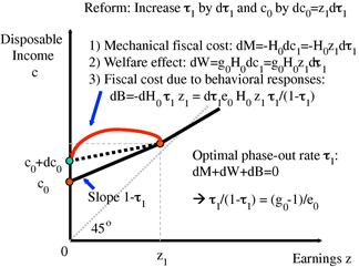
Figure 7 Optimal bottom marginal tax rate with only intensive labor supply responses. The figure, adapted from Diamond and Saez (2011), depicts the derivation of the optimal marginal tax rate at the bottom in the discrete Mirrlees (1971) model with labor supply responses along the intensive margin only. Let ![]() be the fraction of the population not working. This is a function of
be the fraction of the population not working. This is a function of ![]() , the net-of-tax rate at the bottom, with elasticity
, the net-of-tax rate at the bottom, with elasticity ![]() . We consider a small reform around the optimum: The government increases the maximum transfer by
. We consider a small reform around the optimum: The government increases the maximum transfer by ![]() by increasing the phase-out rate by
by increasing the phase-out rate by ![]() leaving the tax schedule unchanged for those with income above
leaving the tax schedule unchanged for those with income above ![]() . This creates three effects which cancel out at the optimum. At the optimum, we have
. This creates three effects which cancel out at the optimum. At the optimum, we have ![]() or
or ![]() . Under standard redistributive preferences,
. Under standard redistributive preferences, ![]() is large implying that
is large implying that ![]() is large.
is large.
First, if society values redistribution toward zero earners, then ![]() is likely to be large (relative to 1). In that case,
is likely to be large (relative to 1). In that case, ![]() is going to be high even if the elasticity
is going to be high even if the elasticity ![]() is large. For example, if
is large. For example, if ![]() and
and ![]() then
then ![]() , a very high phase-out rate. The intuition is simple: increasing transfers by increasing the phase-out rate is valuable if
, a very high phase-out rate. The intuition is simple: increasing transfers by increasing the phase-out rate is valuable if ![]() is large, the fiscal cost due to the behavioral response is relatively modest as those dropping out of the labor force would have had very modest earnings anyway. The phase-out rate is highest in the Rawlsian case where all the social welfare weight is concentrated at the bottom.86
is large, the fiscal cost due to the behavioral response is relatively modest as those dropping out of the labor force would have had very modest earnings anyway. The phase-out rate is highest in the Rawlsian case where all the social welfare weight is concentrated at the bottom.86
Second and conversely, if society considers that non-workers are primarily free-loaders taking advantage of transfers, then ![]() is conceivable. In that case, the optimal phase-out rate is negative and the government provides higher transfers for low income earners rather than those out-of-work. Naturally, this cannot happen under the standard assumption where social marginal welfare weights decrease with income.
is conceivable. In that case, the optimal phase-out rate is negative and the government provides higher transfers for low income earners rather than those out-of-work. Naturally, this cannot happen under the standard assumption where social marginal welfare weights decrease with income.
Finally, note that it is not possible to obtain an explicit formula for the optimal demogrant ![]() as the demogrant is determined in general equilibrium. This is a general feature of optimal tax problems (in the optimal linear tax rate, the demogrant was also deduced from the optimal tax rate
as the demogrant is determined in general equilibrium. This is a general feature of optimal tax problems (in the optimal linear tax rate, the demogrant was also deduced from the optimal tax rate ![]() using the government budget constraint).
using the government budget constraint).
5.3.2 Extensive Margin Responses
The optimality of a traditional means-tested transfer program with a high phase-out rate depends critically on the assumption of intensive labor supply responses. Empirically however, there is substantial evidence that labor supply responses, particularly among low income earners, are also substantial along the extensive margin with less compelling evidence of intensive marginal labor supply response.87 In that case, it is optimal to give higher transfers to low income workers rather than non-workers, which amounts to a negative phase-out rate, as with the current Earned Income Tax Credit (Diamond, 1980; Saez, 2002a).
To see this, consider now a model where behavioral responses of low- and mid-income earners take place through the extensive elasticity only, i.e., whether or not to work, and that earnings when working do not respond to marginal tax rates. Within the general discrete model developed in Section 5.2.2, the extensive model can be obtained by assuming that each individual can only work in one occupation or be unemployed. This can be embodied in the individual utility functions by assuming that ![]() for all occupations
for all occupations ![]() except the one corresponding to the skill of the individual. This structure implies that the fraction of the population
except the one corresponding to the skill of the individual. This structure implies that the fraction of the population ![]() working in occupation
working in occupation ![]() depends only on
depends only on ![]() and
and ![]() for
for ![]() . As a result, and using the fact that
. As a result, and using the fact that ![]() , and defining the elasticity of participation
, and defining the elasticity of participation ![]() , Eq. (12) becomes,
, Eq. (12) becomes,
![]() (15)
(15)
To obtain this result, as depicted on Figure 8, suppose the government starts from a transfer scheme with a positive phase-out rate ![]() and introduces an additional small in-work benefit
and introduces an additional small in-work benefit ![]() that increases net transfers to low income workers earning
that increases net transfers to low income workers earning ![]() . Let
. Let ![]() be the fraction of low income workers with earnings
be the fraction of low income workers with earnings ![]() . The reform has again three effects.
. The reform has again three effects.
Figure 8 Optimal bottom marginal tax rate with extensive labor supply responses. The figure, adapted from Diamond and Saez (2011), depicts the derivation of the optimal marginal tax rate at the bottom in the discrete model with labor supply responses along the extensive margin only. Starting with a positive phase-out rate ![]() , the government introduces a small in-work benefit
, the government introduces a small in-work benefit ![]() . Let
. Let ![]() be the fraction of low income workers with earnings
be the fraction of low income workers with earnings ![]() , and let
, and let ![]() be the elasticity of
be the elasticity of ![]() with respect to the participation net-of-tax rate
with respect to the participation net-of-tax rate ![]() . The reform has three standard effects: mechanical fiscal cost
. The reform has three standard effects: mechanical fiscal cost ![]() , social welfare gain,
, social welfare gain, ![]() , and tax revenue gain due to behavioral responses
, and tax revenue gain due to behavioral responses ![]() . If
. If ![]() , then
, then ![]() . If
. If ![]() , then
, then ![]() implying that
implying that ![]() cannot be optimal. The optimal
cannot be optimal. The optimal ![]() is such that
is such that ![]() implying that
implying that ![]() .
.
First, the reform has a mechanical fiscal cost ![]() for the government. Second, it generates a social welfare gain,
for the government. Second, it generates a social welfare gain, ![]() where
where ![]() is the marginal social welfare weight on low income workers with earnings
is the marginal social welfare weight on low income workers with earnings ![]() . Third, there is a tax revenue gain due to behavioral responses
. Third, there is a tax revenue gain due to behavioral responses ![]() . If
. If ![]() , then
, then ![]() . In that case, if
. In that case, if ![]() , then
, then ![]() , implying that
, implying that ![]() cannot be optimal. The optimal
cannot be optimal. The optimal ![]() is such that
is such that
![]()
implying that the optimal phase-out rate at the bottom is given by:
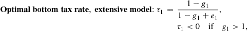 (16)
(16)
Intuitively, starting with a transfer system with a positive phase-out rate as depicted on Figure 8 and ignoring behavioral responses, an in-work benefit reform depicted on Figure 8 is desirable if the government values redistribution to low income earners. If behavioral responses are solely along the extensive margin, this reform induces some non-workers to start working to take advantage of the in-work benefit. However, because we start from a situation with a positive phase-out rate, this behavioral response increases tax revenue as low income workers still end up receiving a smaller transfer than non-workers. Hence, the in-work benefit increases social welfare implying that a positive phase-out rate cannot be optimal.88 Another way to see this is the following. Increasing ![]() distorts the labor supply decision of all types of workers who might quit working. In contrast, increasing
distorts the labor supply decision of all types of workers who might quit working. In contrast, increasing ![]() distorts labor supply of low-skilled workers only. Hence an in-work benefit is less distortionary than an out-of-work benefit in the pure extensive model.
distorts labor supply of low-skilled workers only. Hence an in-work benefit is less distortionary than an out-of-work benefit in the pure extensive model.
5.3.3 Policy Practice
In practice, both extensive and intensive elasticities are present. An intensive margin response would induce those earning slightly more than the minimum to reduce labor supply to take advantage of the in-work benefit, thus reducing tax revenue. Therefore, the government has to trade off the two effects. If, as empirical studies show (see e.g., Blundell & MaCurdy, 1999 for a survey), the extensive elasticity of choosing whether to participate in the labor market is large relative to the intensive elasticity of choosing how many hours to work, initially low (or even negative) phase-out rates combined with high positive phase-out rates further up the distribution would be the optimal profile.
In recent decades in most OECD countries, a concern arose that traditional welfare programs overly discouraged work and there has been a marked shift toward lowering the marginal tax rate for low earners through a combination of: (a) introduction and then expansion of in-work benefits such as the Earned Income Tax Credit in the United States or the Family Credit in the United Kingdom;89 (b) reduction of the statutory phase-out rates in transfer programs for earned income as under the U.S. welfare reform; and (c) reduction of payroll taxes for low income earners.90 Those reforms are consistent with the logic of the optimal tax model we have outlined, as they both encourage labor force participation and provide transfers to low income workers seen as a deserving group. As we saw on Figure 2, the current US system imposes marginal tax rates close to zero on the first $15,000 of earnings but significantly higher marginal rates between $15,000 and $30,000.
How can we explain however that means-tested social welfare programs with high phase-out rates were widely used in prior decades? Historically, most means-tested transfer programs started as narrow programs targeting specific groups deemed unable to earn enough such as widows with children, the elderly, or the disabled. For example, the ancestor of the traditional US welfare program (Aid for Families with Dependent Children, renamed Temporary Aid for Needy Families after the 1996 welfare reform) were “mothers’ pensions” state programs providing help primarily to widows with children and no resources (Katz, 1996). If beneficiaries cannot work but differ in terms of unearned income (for example, the presence of a private pension), then the optimal redistribution scheme is indeed a transfer combined with a 100% phasing-out rate. As governments expanded the scope of transfers, a larger fraction of beneficiaries were potentially able to work. The actual tax policy response to this moral hazard problem over the last few decades has been remarkably close to the lessons from optimal tax theory we have outlined.
Note that following the Reagan and Thatcher conservative revolutions two other elements likely played a role in the shift from traditional means-tested programs toward in-work benefits. First, it is conceivable that society has less tolerance for non-workers living off government transfers because it believes, rightly or wrongly, that most of such non-workers could actually work and earn a living on their own absent government transfers. This means that the social welfare weights on non-workers has fallen relative to the social welfare weights on workers, and especially low income workers. This effect can be captured in our model simply assuming that social welfare weights change (see Section 7 for a discussion of how social welfare weights could be formed in non-utilitarian contexts). Second and related, the perception that relying on transfers generates negative externalities on children or neighbors through a “culture of welfare dependency” might have increased. Such externalities are not incorporated in our basic model but could conceivably be added. In both cases, perceptions of the public and actual facts do not necessarily align (see e.g., Bane & Ellwood, 1994 for a detailed empirical analysis).
6 Extensions
6.1 Tagging
We have assumed that ![]() depends only on earnings
depends only on earnings ![]() . In reality, the government can observe many other characteristics (denoted by vector
. In reality, the government can observe many other characteristics (denoted by vector ![]() ) also correlated with ability (and hence social welfare weights), such as gender, race, age, disability, family structure, height, etc. Hence, the government could set
) also correlated with ability (and hence social welfare weights), such as gender, race, age, disability, family structure, height, etc. Hence, the government could set ![]() and use the characteristic
and use the characteristic ![]() as a “tag” in the tax system. There are two noteworthy theoretical results.
as a “tag” in the tax system. There are two noteworthy theoretical results.
First, if characteristic ![]() is immutable then there should be full redistribution across groups with different
is immutable then there should be full redistribution across groups with different ![]() . This can be seen as follows. Suppose
. This can be seen as follows. Suppose ![]() is a binary 0–1 variable. If the average social marginal welfare weight for group 1 is higher than for group 0, a lump sum tax on group 0 funding a lump sum transfer on group 1 will increase total social welfare.
is a binary 0–1 variable. If the average social marginal welfare weight for group 1 is higher than for group 0, a lump sum tax on group 0 funding a lump sum transfer on group 1 will increase total social welfare.
Second, if characteristic ![]() is not immutable, i.e., it can be manipulated through cheating,91 then it is still desirable to make taxes depend on
is not immutable, i.e., it can be manipulated through cheating,91 then it is still desirable to make taxes depend on ![]() (in addition to
(in addition to ![]() ). At the optimum however, the redistribution across the
). At the optimum however, the redistribution across the ![]() groups will not be complete. To see this, suppose again that
groups will not be complete. To see this, suppose again that ![]() is a binary 0–1 variable and that we start from a pure income tax
is a binary 0–1 variable and that we start from a pure income tax ![]() . As
. As ![]() is correlated with ability, the average social marginal welfare weight for group 1 is different from the one for group 0. Let us assume it is higher. In that case, a small lump sum transfer from group 0 to group 1 increases social welfare, absent any behavioral response. As
is correlated with ability, the average social marginal welfare weight for group 1 is different from the one for group 0. Let us assume it is higher. In that case, a small lump sum transfer from group 0 to group 1 increases social welfare, absent any behavioral response. As ![]() is no longer immutable, this small transfer might induce some individuals to switch from group
is no longer immutable, this small transfer might induce some individuals to switch from group ![]() to group
to group ![]() . However, because we start from a unified tax system, at the margin those who switch do not create any first order fiscal cost (nor any welfare cost through the standard envelope theorem argument).92
. However, because we start from a unified tax system, at the margin those who switch do not create any first order fiscal cost (nor any welfare cost through the standard envelope theorem argument).92
Those points on tagging have been well known in the literature for decades following the analysis of Akerlof (1978) and Nichols and Zeckhauser (1982) for tagging disadvantaged groups for welfare benefits. It has received recent attention in Mankiw and Weinzierl (2010) and Weinzierl (2011) who use the examples of height and age respectively to argue that the standard utilitarian maximization framework fails to incorporate important elements of real tax policy design.
Indeed, in reality, actual tax systems depend on a very limited set of characteristics besides income. Those characteristics are primarily family structure (in particular the number of dependent children), disability status (for permanent and temporary disability programs). Hence, characteristics used reflect direct “need” (for example, the size of the household relative to income), or direct “ability-to-earn” (as is the case with disability status). To the best of our knowledge, the case for using indirect tags correlated with ability in the tax or transfer system has never been made in practice in the policy debate, implying that society does have a strong aversion for using indirect tags. We come back to this issue in Section 7 when we discuss the limits of utilitarianism.
6.2 Supplementary Commodity Taxation
The government can also implement differentiated commodity taxation in addition to nonlinear income taxes and transfers. The usual hypothesis is that commodity taxes have to be linear because of retrading (see e.g., Guesnerie, 1995, Chapter 1). The most common form of commodity taxation, value added taxes and general sales taxes, do display some variation in rates across goods, with exemptions for specific goods, such as food or housing. Such exemptions are in general justified on redistributive grounds. The government also imposes additional taxes on specific goods such as gasoline, tobacco, alcohol, airplane tickets, or motor vehicles.93 Here, we want to analyze whether it is desirable to supplement the optimal nonlinear labor income tax with differentiated linear commodity taxation.
Consider a model with ![]() consumption goods
consumption goods ![]() with pre-tax prices
with pre-tax prices ![]() . Individual
. Individual ![]() derives utility from the
derives utility from the ![]() consumption goods and earnings supply according to a utility function
consumption goods and earnings supply according to a utility function ![]() . The question we want to address is whether the government can increase social welfare using differentiated commodity taxation
. The question we want to address is whether the government can increase social welfare using differentiated commodity taxation ![]() in addition to nonlinear optimal income tax on earnings
in addition to nonlinear optimal income tax on earnings ![]() . Naturally, adding fiscal tools cannot reduce social welfare. However, Atkinson and Stiglitz (1976) demonstrated the following.
. Naturally, adding fiscal tools cannot reduce social welfare. However, Atkinson and Stiglitz (1976) demonstrated the following.
Atkinson-Stiglitz Theorem. Commodity taxes cannot increase social welfare if utility functions are weakly separable in consumption goods vs. leisure and the subutility of consumption goods is the same across individuals, i.e., ![]() with the subutility function
with the subutility function ![]() homogenous across individuals.
homogenous across individuals.
The original proof by Atkinson and Stiglitz (1976) was based on optimum conditions and not intuitive. Recently, Laroque (2005) and Kaplow (2006) have simultaneously and independently proposed a much simpler and intuitive proof that we present here.
Proof. The idea of the proof is that a tax system ![]() that includes both a nonlinear income tax and a vector of commodity taxes can be replaced by a pure income tax
that includes both a nonlinear income tax and a vector of commodity taxes can be replaced by a pure income tax ![]() that keeps all individual utilities constant and raises at least as much tax revenue.
that keeps all individual utilities constant and raises at least as much tax revenue.
Let ![]() subject to
subject to ![]() be the indirect utility of consumption goods common to all individuals. Consider replacing
be the indirect utility of consumption goods common to all individuals. Consider replacing ![]() with
with ![]() where
where ![]() is defined such that
is defined such that ![]() . Such a
. Such a ![]() naturally exists (and is unique) as
naturally exists (and is unique) as ![]() is strictly increasing in
is strictly increasing in ![]() . This implies that
. This implies that ![]() for all
for all ![]() . Hence, both the utility and the labor supply choice are unchanged for each individual
. Hence, both the utility and the labor supply choice are unchanged for each individual ![]() .
.
By definition of an indirect utility, attaining utility of consumption ![]() at price
at price ![]() costs at least
costs at least ![]() . Let
. Let ![]() be the consumer choice of individual
be the consumer choice of individual ![]() under the initial tax system
under the initial tax system ![]() . Individual
. Individual ![]() attains utility
attains utility ![]() when choosing
when choosing ![]() . Hence
. Hence ![]() . As
. As ![]() , we have
, we have ![]() , i.e., the government collects more taxes with
, i.e., the government collects more taxes with ![]() which completes the proof. QED.
which completes the proof. QED.
Intuitively, with separability and homogeneity, conditional on earnings ![]() , the consumption choices
, the consumption choices ![]() do not provide any information on ability. Hence, differentiated commodity taxes
do not provide any information on ability. Hence, differentiated commodity taxes ![]() create a tax distortion with no benefit and it is better to do all the redistribution with the individual nonlinear income tax. With the weaker linear income taxation tool, stronger assumptions on preferences, namely linear Engel curves uniform across individuals, are needed to obtain the commodity tax result (Deaton 1979).94 Intuitively, in the linear tax case, unless Engel curves are linear, commodity taxation can be useful to “non-linearize” the tax system.
create a tax distortion with no benefit and it is better to do all the redistribution with the individual nonlinear income tax. With the weaker linear income taxation tool, stronger assumptions on preferences, namely linear Engel curves uniform across individuals, are needed to obtain the commodity tax result (Deaton 1979).94 Intuitively, in the linear tax case, unless Engel curves are linear, commodity taxation can be useful to “non-linearize” the tax system.
Heterogeneous Preferences.Saez (2002b) shows that the Atkinson-Stiglitz theorem can be naturally generalized to cases with heterogeneous preferences. No tax on commodity ![]() is desirable under three assumptions: (a) conditional on income
is desirable under three assumptions: (a) conditional on income ![]() , social marginal welfare weights are uncorrelated with the levels of consumption of good
, social marginal welfare weights are uncorrelated with the levels of consumption of good ![]() , (b) conditional on income
, (b) conditional on income ![]() , the behavioral elasticities of earnings are uncorrelated with the consumption of good
, the behavioral elasticities of earnings are uncorrelated with the consumption of good ![]() , and (c) at any income level
, and (c) at any income level ![]() , the average individual variation in consumption of good
, the average individual variation in consumption of good ![]() with
with ![]() is identical to the cross-sectional variation in consumption of good
is identical to the cross-sectional variation in consumption of good ![]() with
with ![]() .
.
Assumption (a) is clearly necessary and might fail when earnings ![]() is no longer a sufficient statistic for measuring welfare. For example, if some individuals face high uninsured medical expenses due to poor health, then this assumption would not hold, and it would be desirable to subsidize health expenditures.95 However, when heterogeneity in consumption reflects heterogeneity in preferences and not in need, assumption (a) is a natural assumption.
is no longer a sufficient statistic for measuring welfare. For example, if some individuals face high uninsured medical expenses due to poor health, then this assumption would not hold, and it would be desirable to subsidize health expenditures.95 However, when heterogeneity in consumption reflects heterogeneity in preferences and not in need, assumption (a) is a natural assumption.
Assumption (b) is a technical assumption required to ensure that consumption of specific goods is not a tag for low responsiveness of labor supply to taxation. For example, if consumers of luxury cars happened to have much lower labor supply elasticities than average, it would become efficient to tax luxury cars as a way to indirectly tax more the earnings of those less responsive individuals. In practice, too little is known about the heterogeneity in labor supply across individuals to exploit such possibilities. Hence, assumption (b) is also a natural assumption.
Assumption (c) is the critical assumption. When it fails, the thought experiment to decide on whether commodity ![]() ought to be taxed is the following. Suppose high ability individuals are forced to work less and earn only as much as lower ability individuals. In that scenario, if higher ability individuals consume more of good
ought to be taxed is the following. Suppose high ability individuals are forced to work less and earn only as much as lower ability individuals. In that scenario, if higher ability individuals consume more of good ![]() than lower ability individuals, then taxing good
than lower ability individuals, then taxing good ![]() is desirable. This can happen for two reasons. First, high ability people may have a relatively higher taste for good
is desirable. This can happen for two reasons. First, high ability people may have a relatively higher taste for good ![]() (independently of income) in which case taxing good
(independently of income) in which case taxing good ![]() is a form of indirect tagging of high ability. Second, good
is a form of indirect tagging of high ability. Second, good ![]() is positively related to leisure, i.e., consumption of good
is positively related to leisure, i.e., consumption of good ![]() increases when leisure increases keeping after-tax income constant. This suggests taxing more holiday-related expenses and subsidizing work-related expenses such as child care.
increases when leisure increases keeping after-tax income constant. This suggests taxing more holiday-related expenses and subsidizing work-related expenses such as child care.
In general the Atkinson-Stiglitz assumption is a good starting place for most goods. This implies that lower or zero VAT rates on some goods for redistribution purposes is inefficient (in addition to being administratively burdensome). Under those assumptions, eliminating such preferential rates and replacing them with a more redistributive income tax and transfer system would increase social welfare.96
6.3 In-Kind Transfers
As we discussed in Section 3, the largest transfer programs are in-kind rather than cash. OECD countries in general provide universal public health care benefits and public education. They also often provide in-kind housing or nutrition benefits on a means-tested basis.
As is well known, from a rational individual perspective, if the in-kind benefit is tradable, it is equivalent to cash. Most in-kind benefits however are not tradable. In that case, recipients may be forced to overconsume the good provided in-kind and would instead prefer to receive the cash equivalent value of the in-kind transfer. Therefore, from a narrow rational individual perspective, cash transfers dominate in-kind transfers. From a social perspective, three broad lines of justification have been provided in favor of in-kind benefits.97
1. Commodity Egalitarianism: A number of goods, such as education or health care are seen as rights everybody in society is entitled to.98 Those goods are hence put in the same category as other rights that democratic governments offer to all citizens without distinction such as protection under the law, free speech, right to vote, etc. The difficulty with this view is that it does not say which level of education or health care should be seen as a right.
2. Paternalism: The government might want to impose its preferences on transfer recipients. For example, voters might support providing free shelter and free meals to the homeless but would oppose giving them cash that might be used for alcohol or tobacco consumption. In that case, recipients would rather get the cash equivalent value of the non-cash transfers they get but society’s paternalistic views prevail upon recipients’ preferences. Those arguments have been developed mostly by libertarians to criticize in-kind benefits (e.g., Milton Friedman was favorable to basic redistribution through a negative income tax cash transfer rather than in-kind benefits).
3. Individual Failures: Related, recipients could themselves realize that, if provided with only cash, they might choose too little health care, education, or retirement savings for their long-term well being, perhaps because of lack of information or self-control problems (e.g., hyperbolic discounting is an elegant way to model such self-control issues). In this case, recipients understand that non-cash benefits are in their best interest. Hence, recipients would actually support getting such non-cash benefits instead of the equivalent cash value. This type of rationalization for non-cash transfers hence differs drastically from the paternalistic view. The fact that all advanced economies systematically provide large amounts of non-cash benefits universally (retirement, health, education) through a democratic process is more consistent with the “individual failures” scenario than the “paternalism” scenario. The case of education, and especially primary education, is particularly important. Children cannot be expected to have fully forward looking rational preferences. Parents make educational choices on behalf of their children and most—but not all—parents have the best interests of their children at heart. Compulsory and free public education is a simple way for the government to ensure that all children get a minimum level of education regardless of how caring their parents are.
4. Second-best Efficiency: A number of studies have shown that, with limited information and limited policy tools, non-cash benefits can actually be desirable in a “second-best” equilibrium. In-kind benefits can be used by the government to relax the incentive constraint created by the optimal tax problem. This point was first noted by Nichols and Zeckhauser (1982) and later developed in a number of studies (see Currie & Gahvari, 2008 and Boadway, 2012, Chapter 4 for detailed surveys). Those results are closely related to the Atkinson and Stiglitz (1976) theorem presented above. If the utility function is not separable between consumption goods and leisure, then we know that commodity taxation is useful to supplement optimal nonlinear earnings taxation. By the same token, it can be shown that providing an in-kind transfer of a good complementary with work is desirable because it makes it relatively more costly for high skill people to work less. Although such “second-best” arguments have attracted the most attention in the optimal tax literature, they are second order in the public debate which focuses primarily on the other justifications we discussed above.
6.4 Family Taxation
In practice, the treatment of families raises important issues. Any tax and transfer system must make a choice on how to treat singles vs. married households and how to make taxes and transfers depend on the number of children. There is relatively little normative work on those questions, in large part because the standard utilitarian framework is not successful at capturing the key trade offs. Kaplow (2008), Chapter 8 provides a detailed review.
Couples. Any income tax system needs to decide how to treat couples vs. single individuals. As couples typically share resources, welfare is best measured by family income rather than individual income. There are two main treatments of the family in actual tax (or transfer) systems. (a) The individual system where every person is taxed separately based on her individual income. In that case, couples are treated as two separate individuals. As a result, an individual system does not impose any tax or subsidy on marriage as tax liability is independent of living arrangements. At the same time, it taxes in the same way a person married to a wealthy spouse vs. a person married to a spouse with no income. (b) The family system where the income tax is based on total family income, i.e., the sum of the income of both spouses in case of married couples. The family system can naturally modulate the tax burden based on total family resources, which best measures welfare under complete sharing within families. However and as a result, a family tax system with progressive tax brackets cannot be neutral with respect to living arrangements, creating either a marriage tax or a marriage subsidy. Under progressive taxation, if the tax brackets for married couples are the same as for individuals, the family system typically creates a marriage tax. If the tax brackets for married couple are twice as wide as for individuals, the family system typically creates a marriage subsidy.99
Hence and as is well known, it is impossible to have a tax system that simultaneously meets three desirable properties: (1) the tax burden is based on family income, (2) the tax system is marriage neutral, and (3) the tax system is progressive (i.e., the tax system is not strictly linear). Although those properties clearly matter in the public debate, it is not possible to formalize their trade off within the traditional utilitarian framework as the utilitarian principle cannot put a weight on the marriage neutrality principle.
If marriage responds strongly to any tax penalty or subsidy, it is better to reduce the marriage penalty/subsidy and move toward an individualized system. This issue might be particularly important in countries (such as Scandinavian countries for example), where many couples cohabit without being formally married and as it is difficult (and intrusive) for the government to observe (and monitor) cohabitation status.
Traditionally, the labor supply of secondary earners—typically married women—has been found to be more elastic than the labor supply of primary earners—typically married men (see Blundell & MaCurdy, 1999 for a survey). Under the standard Ramsey taxation logic, this implies that it is more efficient to tax secondary earners less (Boskin & Sheshinski, 1983). If the tax system is progressive, this goal is naturally achieved under an individual-based system as secondary earners are taxed on their sole earnings. Note however that the difference in labor supply elasticities between primary and secondary earners has likely declined over time as more and more married women work (Blau & Kahn, 2007).
In practice, most OECD countries have switched from family based to individual-based income taxation. In contrast, transfer systems remain based on family income. It is therefore acceptable to the public that a spouse with modest earnings would face a low tax rate, no matter how high the earnings of her/his spouse are.100 In contrast, it appears unacceptable to the public that a spouse with modest earnings should receive means-tested transfers if the earnings of his or her spouse are high. A potential explanation could be framing effects as direct transfers might be more salient than an equivalent reduction in taxes. Kleven, Kreiner, and Saez (2009b) offer a potential explanation in a standard utilitarian model with labor supply where they show that the optimal joint tax system is to have transfers for non-working spouses (or equivalently taxes on secondary earnings) that decrease with primary earnings. The intuition is the following. With concave utilities, the presence of secondary earnings make a bigger difference in welfare when primary earnings are low than when primary earnings are large. Hence, it is more valuable to compensate one earner couples (relative to two earner couples) when primary earnings are low. This translates into an implicit tax on secondary earnings that decreases with primary earnings. Such negative jointness in the tax system is approximately achieved by having family based means-tested transfers along with individually based income taxation.
Children. Most tax and transfer systems offer tax reductions for children or increases in benefits for children. The rationale for such transfers is simply that, conditional on income ![]() , families with more children are more in need of transfers and have less ability to pay taxes. The interesting question that arises is how the net transfer (additional child benefits or reduction in taxes) per additional child should vary with income
, families with more children are more in need of transfers and have less ability to pay taxes. The interesting question that arises is how the net transfer (additional child benefits or reduction in taxes) per additional child should vary with income ![]() . On the one hand, the need for children related transfers is highest for families with very small incomes. On the other hand, the cost of children is higher for families with higher incomes particularly when parents work and need to purchase childcare.
. On the one hand, the need for children related transfers is highest for families with very small incomes. On the other hand, the cost of children is higher for families with higher incomes particularly when parents work and need to purchase childcare.
Actual tax and transfers do seem to take both considerations into account. Means-tested transfers tend to offer child benefits that are phased-out with earnings. Income taxes tend to offer child benefits that increase with income for two reasons. First, the lowest income earners do not have taxable income and hence do not benefit from child-related tax reductions. Second, child-related tax reductions are typically a fixed deduction from taxable income which is more valuable in upper income tax brackets. Hence, the level of child benefits tends to be U-shaped as a function of earnings. Two important qualifications should be made.
First, as mentioned in Section 5.3.3, a number of countries have introduced in-work benefits that are tied to work and presence of children. This tends to make child benefits less decreasing with income at the low income end. In the United States, because of the large EITC and child tax credits and small traditional means-tested transfers, the benefit per child is actually increasing with family earnings at the bottom. Second, another large child benefit often subsidized or government provided is pre-school child care (infant child care, kindergarten starting at age 2 or 3, etc.). Such child care benefits are quantitatively large and most valuable when both parents work or for single working parents. Hence, economically, they are a form of in-kind in-work benefit which also promotes labor force participation (see OECD, 2006, chap. 4, Figure 4.1, p.129 for an empirical analysis). It is perhaps not a coincidence that cash in-work benefits for children are highest in the US and the UK, countries which provide minimal child care public benefits. Understanding in that context whether a cash transfer or an in-kind child care benefit is preferable is an interesting research question that has received little attention.
Child-related benefits raise two additional interesting issues.
First, families do not take decisions as a single unit (Chiappori, 1988). Interestingly, in the case of children, cash transfers to mothers (or grandmothers) have larger impacts on children’s consumption than transfers to fathers. This has been shown in the UK context (Lundberg, Pollak, & Wales, 1997) when the administration of child tax benefits was changed from a reduction in tax withholdings of parents (often the father) to a direct check to the mother. Similar effects have been documented in the case of cash benefits for the elderly in South Africa (Duflo, 2003). This evidence suggests that in-kind benefits (such as child care or pre-school) might be preferable if the goal is to ensure that resources go toward children. As mentioned above, primary education is again the most important example of in-kind benefits designed so that children benefit regardless of how caring parents are.
Second, child benefits might promote fertility. A large empirical literature has found that child benefits have sometimes positive but in general quite modest effects on fertility (see Gauthier, 2007 for a survey). There can be externalities (both positive and negative) associated with children. For example, there can be congestion effects (such as global warming) associated with larger populations. Alternatively, declines in populations can have adverse effects on sustainability of pay-as-you-go pension arrangements. Such externalities should be factored into discussions of optimal child benefits.
6.5 Relative Income Concerns
Economists have long been interested in the possibility that individuals care not only about their absolute income but also their income relative to others. Recently, substantial evidence coming from observational studies (e.g., Luttmer, 2005), lab experiments (e.g., Fehr & Schmidt, 1999), and field experiments (Card, Mas, Moretti, & Saez 2012), provide support for relative income effects. A number of optimal tax studies have incorporated relative income in the analysis (Boskin & Sheshinski, 1978 analyze the linear income tax case and Oswald, 1983 and Tuomala, 1990, Chapter 8 consider the nonlinear income tax case). Those studies find that in general relative income concerns tend to increase optimal tax rates. Relative income effects can be modeled in a number of ways. The simplest way, which we consider here, is to posit that individual utility also depends on the utility of others.101
Relative income concerns affect optimal tax analysis in two ways. First, it changes the social marginal welfare weights as a decrease in the utility of others has a direct effect on one’s utility (keeping one’s work and income situation constant), creating externalities. In our view, the simplest way to capture this effect is to consider that those externalities affect the social welfare weights. If a decrease in a person’s income increases others’ utility, then the social welfare weight on this person ought to be reduced by this external effect. Whether such externalities should be factored in the social welfare function is a deep and difficult question. Surely, hurting somebody with higher taxes for the sole satisfaction of envy seems morally wrong, Hence, social welfare weights should not be allowed to be negative for anybody no matter how strong the envy effects. At the same, it seems to us that relative income concerns are a much more powerful and realistic way to justify social welfare weights decreasing with income than standard utilitarianism with concave utility of consumption.
Second, relative income concerns affect labor supply decisions. For example, if utility functions are such that ![]() with
with ![]() average consumption in the economy, then a proportional tax on consumption affects
average consumption in the economy, then a proportional tax on consumption affects ![]() and
and ![]() equally and hence has no impact on labor supply. This might be a simple explanation for why labor supply is relatively inelastic with respect to secular increases in wage rates over the long-term process of economic growth (Ramey and Francis, 2009).102 This labor supply channel effect is fully captured by the behavioral response elasticity and hence does not change the optimal tax formulas.
equally and hence has no impact on labor supply. This might be a simple explanation for why labor supply is relatively inelastic with respect to secular increases in wage rates over the long-term process of economic growth (Ramey and Francis, 2009).102 This labor supply channel effect is fully captured by the behavioral response elasticity and hence does not change the optimal tax formulas.
As an illustration, let us go back to the optimal top tax rate analysis from Section 5.1 with a small variation ![]() in the top tax rate. The key difference in the analysis is that the reduction in welfare for top bracket earners would now have a positive externality on the utility of lower income individuals. As long as this external effect is weakly separable from labor supply choices, i.e.,
in the top tax rate. The key difference in the analysis is that the reduction in welfare for top bracket earners would now have a positive externality on the utility of lower income individuals. As long as this external effect is weakly separable from labor supply choices, i.e., ![]() where
where ![]() is the standard utility function and
is the standard utility function and ![]() is the vector of utilities of all other (non
is the vector of utilities of all other (non ![]() ) individuals, the individual earnings
) individuals, the individual earnings ![]() decisions are not affected by the external effect. The external effect is proportional to the direct welfare effect on top bracket earners and the strength of the externality. Therefore, the external effect simply reduces the social marginal value of consumption of top bracket earners from
decisions are not affected by the external effect. The external effect is proportional to the direct welfare effect on top bracket earners and the strength of the externality. Therefore, the external effect simply reduces the social marginal value of consumption of top bracket earners from ![]() to
to ![]() . The optimal tax formula retains the same form as before
. The optimal tax formula retains the same form as before ![]() .
.
In sum, we think that relative income concerns are a useful way to interpret and justify optimal tax analysis and can be incorporated within standard optimal tax analysis.
6.6 Other Extensions
Endogenous Wages. The standard assumption in optimal labor income tax theory is that pre-tax wage rates are exogenous, i.e., that there is perfect substitutability between skills in production. Interestingly, in the discrete occupational models we have introduced in Section 5.2.2, this assumption can be relaxed without affecting the general optimal tax formula (12). To see this, consider a general production function ![]() of the consumption good with constant returns to scale.103 In that case, wages are set by marginal product
of the consumption good with constant returns to scale.103 In that case, wages are set by marginal product ![]() . The maximization of the government can be rewritten as choosing
. The maximization of the government can be rewritten as choosing ![]() to maximize
to maximize
![]()
Note that any explicit reference to wages ![]() has disappeared from this maximization problem and the first order condition with respect to
has disappeared from this maximization problem and the first order condition with respect to ![]() immediately leads to the same optimal tax formula (12).
immediately leads to the same optimal tax formula (12).
The intuition in a basic two skill model is the following. Suppose an increase in high skill taxes leads to a reduction in high skill labor supply and hence an increase in high skill wages (and a decrease in low skill wages) through demand effects. Because of the absence of profits, those demand effects are a pure transfer from low to high skill workers. Therefore, the government can readjust the tax on high and low skills to offset those demand effects on the net consumption levels at no net fiscal cost, leaving the optimal tax formula unchanged.104
Theoretically, this result arises because the discrete occupational model is effectively mathematically identical to a Diamond and Mirrlees (1971), optimal commodity tax model where each occupation is a specific good taxed at a specific rate. As is well known from Diamond and Mirrlees (1971), optimal Ramsey tax formulas depend solely on consumers’ demand and do not depend on production functions. This generates two important additional consequences. First, the production efficiency result of Diamond and Mirrlees (1971) carries over to the discrete occupational choice model, implying that distortions in the production process or tariffs (in the case of an open economy) are not desirable. Second, in an extended model with many consumption goods, the theorem of Atkinson and Stiglitz (1976) also carries over to the discrete occupational choice model. Namely, differentiated commodity taxation is not desirable to supplement optimal nonlinear earnings taxation under the standard separability assumption presented above. Those results are formally proven in Saez (2004b). They stand in sharp contrast to results obtained in the Stiglitz (1982) discrete model with endogenous wages where it is shown that the optimal tax formulas are affected by endogenous wages (Stiglitz, 1982), and where the production efficiency theorem and the Atkinson-Stiglitz theorem do not carry over (Naito, 1999). Saez (2004b) argues that the occupational model best captures the long-term when individuals choose their occupations while the Stiglitz (1982) model captures a short-term situation where individuals have fixed skills and only adjust hours of work.
Workfare, Take-Up Costs, and Screening. Workfare can be defined as requiring transfer beneficiaries to work, typically for a public project. In its extreme form, the work required has no productive value. In that case, workfare is similar to imposing an ordeal, such as time consuming take-up costs, on welfare beneficiaries. The literature has focused primarily on such “useless workfare requirements.” Besley and Coate (1992) show that, if the government cares about poverty measured by net-income rather than individual utilities, it can be optimal to impose workfare. In their model, workfare screens away higher wage individuals who have a higher opportunity cost of time.105
Cuff (2000) shows, in a standard Stiglitz (1982) two-type discrete model that a useless workfare program is never desirable with a standard welfarist objective. Interestingly, Cuff (2000)then extends the analysis to include heterogeneity in tastes for work (in addition to the standard wage rate heterogeneity). When there are lazy vs. hard working low skill workers and when society does not like to redistribute toward lazy low skill workers, workfare can become desirable. This is because work requirements are more costly to lazy types than hard working types.
In practice, finding ordeals which hurt more the undeserving beneficiaries than the deserving beneficiaries seems difficult. In particular, if society feels that welfare is too generous, it is more efficient to cut benefits directly rather than impose ordeals. Both reduce welfare benefits (and hence the incentives to become a recipient), but at least direct cuts save on government spending.
Screening mechanisms that also impose costs on recipients, (e.g., filing out forms, medical tests, etc.) can be desirable when they are successful in screening deserving recipients (e.g., the truly disabled) vs. undeserving recipients (e.g., those faking disability). Diamond and Sheshinski (1995) propose an analysis along those lines in the case of disability insurance (see also the chapter by Chetty and Finkelstein in this volume for more details on optimal social insurance). The key difference with useless workfare or ordeals is that such screening is directly designed at separating deserving vs. undeserving recipients. It is very unlikely that blanket ordeals can achieve this. Today, data driven screening (i.e., checking administrative databases for potential earnings, etc.) are far more powerful and efficient than direct in person screening (and a lot less intrusive for recipients).
Minimum Wages. The minimum wage is another policy tool that can be used for redistribution toward low skill workers. At the same time minimum wages can create unemployment among low skill workers, creating a trade off between equity and efficiency. A small literature has examined the desirability of minimum wages in addition to optimal taxes and transfers in the standard competitive labor market with endogenous wage rates (as in the model discussed above).106
Lee and Saez (2012) use the occupational model of Section 5.3.2 with endogenous wages and prove two results. First, they show that a binding minimum wage is desirable under the strong assumption that unemployment induced by the minimum wage hits the lowest surplus workers first. The intuition for this result is simple and can be understood using Figure 8. Suppose a minimum wage is set at level ![]() and that transfers to low-skilled workers earning
and that transfers to low-skilled workers earning ![]() are increased. The presence of the minimum wage at
are increased. The presence of the minimum wage at ![]() rations low skill work and effectively prevents the labor supply responses from taking place. Some non-workers would like to work and earn
rations low skill work and effectively prevents the labor supply responses from taking place. Some non-workers would like to work and earn ![]() but cannot find jobs because those jobs are rationed by the minimum wage. Therefore, the minimum wage enhances the ability of the government to redistribute (via an EITC type benefit) toward low skill workers.
but cannot find jobs because those jobs are rationed by the minimum wage. Therefore, the minimum wage enhances the ability of the government to redistribute (via an EITC type benefit) toward low skill workers.
Second, when labor supply responses are along the extensive margin only, which is the empirically relevant case, the co-existence of a minimum wage with a positive tax rate on low-skilled work is always (second-best) Pareto inefficient. A Pareto improving policy consists of reducing the pre-tax minimum wage while keeping constant the post-tax minimum wage by increasing transfers to low-skilled workers, and financing this reform by increasing taxes on higher paid workers. Importantly, this result is true whether or not rationing induced by the minimum wage is efficient or not. This result can also rationalize policies adopted in many OECD countries in recent decades that have decreased the minimum wage while reducing the implicit tax on low skill work through a combination of reduced payroll taxes for low skill workers and in-work benefits of the EITC type for low skill workers.
Optimal Transfers in Recessions. In practice, some transfers (such as unemployment insurance in the United States) can be made more generous during recessions. Traditionally, optimal policy over the business cycle has been analyzed in the macro-economics literature rather than the public economics literature.107 The macro-economics literature, however, rarely focuses on distributional issues. There are three channels through which recessions can affect the calculus of optimal transfers for those out-of-work.
First, recessions are a time of high unemployment where people want to work but cannot find jobs. This suggests that employment is limited by demand effects rather than the supply effects of the traditional optimal tax analysis. As a result, in recessions, unemployment is likely to be less sensitive to supply-side changes in search efforts and job search is likely to generate a negative externality on other job seekers in the queue. Landais, Michaillat, and Saez (2010) capture this effect in a search model where job rationing arises in recessions and show that unemployment insurance should be more generous during recessions. Crépon, Esther, Marc, Roland and Philippe (in press), using a large scale job placement aid randomized experiment in France, show that indeed there are negative externalities of job placement aid on other job seekers and that those externalities are larger when unemployment is high.
Second, in recessions, the ability to smooth consumption might be reduced, as the long-term unemployed might exhaust their buffer stock savings and might face credit constraints. This implies that the gap in social marginal utility of consumption between workers and non-workers might grow during recessions, further increasing the value of redistributing from workers to the unemployed (Chetty, 2008).
Third and related, individuals are less likely to be responsible for their unemployment status in a recession than in an expansion. In an expansion when jobs are easy to find, long unemployment spells are more likely to be due to low search efforts than in a recession when jobs are difficult to find even with large search efforts. If society wants to redistributive toward the hard-searching unemployed—i.e., those who would not have found jobs even absent unemployment benefits—then it seems desirable to have time limited benefits during good times combined with expanded benefit durations in bad times. We will come back to such non-utilitarian social preferences in Section 7.
Education Policy. Education plays a critical role in generating labor market skills. All advanced economies provide free public education at the K-12 level and heavily subsidize higher education. As we have seen earlier, there is a strong rationale for providing K-12 public education to correct potential parenting failures. For higher education, the presence of credit constraints might lead to suboptimal educational levels, providing a strong rationale for government provision of loans (see e.g., Lochner and Monge, 2011).108 However, governments in advanced economies not only provide loans but also direct subsidies to higher education. Direct subsidies could be justified by “behavioral considerations” if a significant fraction of young adults are not able to make wise educational choices on their own—due for example to informational or self-control issues.
A small literature in optimal taxation has examined the desirability of education subsidies in fully rational models. Higher education subsidies encourage skill acquisition but tend to benefit more the relatively skilled and hence are likely regressive. Absent any ability to observe educational choices, the total elasticity of earnings with respect to net-of-tax rates is due to both labor supply and education choices. If education choices are elastic, the corresponding optimal income tax should incorporate the full elasticity and not solely the labor supply elasticity. This naturally leads to lower optimal tax rates than those calibrated using solely the labor supply elasticity. Diamond and Mirrlees (Unpublished) develop this point, which they call the “Le Chatelier” principle.109
Suppose now that the government can observe educational choices and hence directly subsidize (or tax) them in addition to using income-based taxes and transfers. In that context, redistributive taxes and transfers discourage both labor supply and education investments as they reduce the net rewards from higher education. Bovenberg and Jacobs (2005) consider such a model and show that combining educational subsidies with redistributive income-based taxation is optimal—consistent with real policies.
In the simplest version of their model, education ![]() increases the wage rate
increases the wage rate ![]() (with
(with ![]() increasing and concave and
increasing and concave and ![]() being innate ability) at a cost
being innate ability) at a cost ![]() . Individuals choose
. Individuals choose ![]() and
and ![]() to maximize utility
to maximize utility ![]() subject to
subject to ![]() where
where ![]() is the income tax rate,
is the income tax rate, ![]() the subsidy rate on education expenses
the subsidy rate on education expenses ![]() , and
, and ![]() the demogrant. In this simple model,
the demogrant. In this simple model, ![]() is an intermediate good that does not directly enter the utility function which depends solely on
is an intermediate good that does not directly enter the utility function which depends solely on ![]() and
and ![]() . The education choice is given by the first order condition
. The education choice is given by the first order condition ![]() . Hence, education is pure cost of production and individuals should be taxed on their earnings net of education costs
. Hence, education is pure cost of production and individuals should be taxed on their earnings net of education costs ![]() . This implies that
. This implies that ![]() should be set exactly equal to
should be set exactly equal to ![]() .
.
7 Limits of the Welfarist Approach and Alternatives
7.1 Issues with the Welfarist Approach
All our analysis so far has followed the standard welfarist approach whereby the government objective is to maximize a weighted sum of individual utilities (or an increasing transformation of utilities). As we saw, all optimal tax formulas can be expressed in terms of the social marginal welfare weights attached to each individual which measure the social value of an extra dollar of consumption to each individual.
In standard optimal tax analysis, the utilitarian case (maximizing the unweighted sum of individual utilities) is by far the most widely used. In that case, social welfare weights are proportional to the marginal utility of consumption. As we have seen, this criterion generates a number of predictions at odds with actual tax systems and with people’s intuitive sense of redistributive justice.
First, if individuals do not respond to taxes, i.e., if pre-tax incomes are fixed, and individual utilities are concave, then utilitarianism recommends a 100% tax, and full redistribution. In reality, even absent behavioral responses, many and perhaps even most people would still object to confiscatory taxation on the grounds that people deserve to keep part of the income they have created.
Second and related, views on taxes and redistribution seem largely shaped by views on whether the income generating process is fair and whether individual incomes are deserved or not. The public tends to dislike the redistribution of fairly earned income through one’s effort but is in favor of redistributing income earned unfairly or due to pure luck (see Piketty, 1995 for a theoretical model and Alesina & Giuliano, 2011, chap. 4 for a recent survey). Such distinctions are irrelevant for utilitarianism.
Third, as we have seen in Section 6.1 on tagging, under utilitarianism, optimal taxes should depend on all observable characteristics which are correlated with intrinsic earning ability. In practice, taxes and transfers use very few of the potentially available tags. Society seems to have horizontal equity concerns and using tags to achieve indirect redistribution is hence perceived to be unfair.
Fourth, perceptions about recipients seem to matter a great deal for the public views on transfers. Most people support transfers for people really unable to work, such as the truly disabled but most people dislike transfers to people able to work and who would work absent transfers. In the standard model, behavioral responses matter for optimal taxes only through their effects on the government budget. In reality, the presence of behavioral responses also colors the public perceptions on how deserving transfer beneficiaries are.
7.2 Alternatives
A number of alternatives to welfarism have been proposed in the literature.
Pareto Principle. First, let us recall that the standard utilitarian criterion can be easily extended, as we have seen, by considering a weighted sum of individual utilities (instead of a simple sum). Those positive weights are called Pareto weights. By changing those weights, we can describe the set of all second-best Pareto efficient tax equilibria. It seems natural that any “optimal tax system” should be at least second-best Pareto efficient, i.e., no feasible tax reform can improve the welfare of everybody. Hence, the Pareto principle imposes a reasonable but weak condition on tax optima. Indeed, optimal tax analysis was particularly interested in finding properties that hold true for all such second-best optima.110 Those properties are relatively few, an example being the Atkinson and Stiglitz theorem. Hence, considering arbitrary weights is not going to be enough to obtain definite conclusions in general. Hence, it is necessary to be able to put more structure on those Pareto weights so that we can select among the wide set of second-best Pareto optimal tax systems.
All the examples of alternatives to utilitarianism we describe next show that any criterion leads to a specific set of marginal social welfare weights.
Rawlsian Criterion. In the Rawlsian criterion, Pareto weights are concentrated solely on the most disadvantaged person in the economy. This amounts to maximizing the utility of the person with the minimum utility, hence this criterion is also called the maxi-min objective. A judgment needs to be made as to who is the most disadvantaged person. In models with homogeneous preferences and heterogeneous skills, the most disadvantaged person is naturally the person with the lowest skill and hence the lowest earnings. This criterion has the appealing feature that, once society agrees on who is the most disadvantaged person, the optimum is independent of the cardinal choice for individual utilities. The key weakness of this criterion is that it concentrates all social welfare on the most disadvantaged and hence represents extreme redistributive tastes. Intuitively, it seems clear that the political process will put weight on a broader set of voters than solely the most disadvantaged. Hence, the Rawlsian principle makes sense politically only if the most disadvantaged form a majority of the population. This is not a realistic assumption in the case of redistribution of labor income.111 For example, we have seen in Section 4.1 that a standard median voter outcome puts all the weight on the median voter preferences.
Libertarianism and Benefits Principle. At the other extreme, libertarians argue that the government should not do any redistribution through taxes and transfers. Therefore, taxes should be set according to the benefits received from government spending, individual by individual. This is known as the benefits principle of taxation. Any redistribution over and above benefits is seen as unjust confiscation of individual incomes. Such a principle can be formally captured by assuming that social marginal welfare weights are identical across individuals (in the situation where taxes correspond to benefits). In that case, additional redistribution does not add to social welfare.112 While some voters may hold libertarian views, as we discussed in Section 2.1, all OECD countries do accomplish very substantial redistribution across individuals, and hence depart very significantly from the benefits principle of taxation. This shows that the benefits principle cannot by itself account for actual tax systems.
Principles of Responsibility and Compensation. The general idea is that individuals should be compensated for circumstances affecting their welfare over which they have no control, such as their family background or disability at birth. This is the principle of compensation. In contrast, individuals should be held responsible for circumstances which they control such as how many hours they work. Hence, no redistribution should take place based on such choices. This is the principle of responsibility. These principles are presented and discussed in detail in Kolm (1996), Roemer (1998), Fleurbaey (2008), Fleurbaey and Maniquet (2011).
An example often presented in the literature is that of individuals differing by their wage rate which they do not control (for example because it is due to exogenous ability), and by their taste for leisure (some people prefer goods consumption, some people prefer leisure consumption). By the principle of compensation, it is fair to redistribute from high wage to low wage individuals. By the principle of responsibility, it is unfair to redistribute from goods lovers toward leisure lovers. When there is only one dimension of heterogeneity, those principles are easy to apply. For example, if individuals differ only according to their wage rate (and not in their tastes), then the principle of compensation boils down to a Rawlsian criterion whereby the tax and transfer system should provide as much compensation as possible to the lowest wage people. In terms of welfarism, social marginal welfare weights are fully concentrated on the lowest wage person. If individuals differ solely in taste for work, the principle of responsibility calls for no redistribution at all because everybody has the same time endowment that they can divide between work and leisure based on their relative tastes for goods consumption vs. leisure consumption. It would be unfair to redistribute based on tastes.113 The standard welfarist approach cannot easily obtain this meaningful result, except through a renormalization of Pareto weights so that social marginal utilities of consumption are the same across individuals (absent transfers).114
However, those two principles can conflict in situations where there is heterogeneity in both dimensions (skills and taste for leisure). Fleurbaey (2004) presents a simple example in a two skill, two levels of taste for leisure model showing that it is not possible to fulfill both the responsibility principle and the compensation principle at the same time. Therefore, some trade off needs to be made between the two principles. This trade-off needs to be specified through a social objective function. Fleurbaey (2008) reviews this literature and the many criteria that have been proposed.115
Equal Opportunity. One prominent example of how to trade-off the responsibility vs. the compensation principles is Roemer (1998) and Roemer et al. (2003) who propose an Equal Opportunity criterion. In the model of Roemer et al. (2003), individuals differ solely in their wage rate ![]() but the wage rate depends in part on family background and in part on merit (i.e., personal effort in getting an education, getting ahead, etc.). The model uses quasi-linear utility functions
but the wage rate depends in part on family background and in part on merit (i.e., personal effort in getting an education, getting ahead, etc.). The model uses quasi-linear utility functions ![]() uniform across individuals. In the model, people are responsible for wage differences due to merit but not for wage differences due to family background. Suppose for simplicity there is a low and high family background. The distribution of wage rates is equal to
uniform across individuals. In the model, people are responsible for wage differences due to merit but not for wage differences due to family background. Suppose for simplicity there is a low and high family background. The distribution of wage rates is equal to ![]() and
and ![]() among those coming from low and high family backgrounds respectively. Assume that high family background provides an advantage so that
among those coming from low and high family backgrounds respectively. Assume that high family background provides an advantage so that ![]() stochastically dominates
stochastically dominates ![]() . The government wants to redistribute from high to low family backgrounds but does not want to redistribute across individuals with different wages within a family background group because their position within the group is due to merit. The government can only observe earnings
. The government wants to redistribute from high to low family backgrounds but does not want to redistribute across individuals with different wages within a family background group because their position within the group is due to merit. The government can only observe earnings ![]() and cannot observe family background (nor the wage rate). Hence, the government is limited to using a nonlinear income tax
and cannot observe family background (nor the wage rate). Hence, the government is limited to using a nonlinear income tax ![]() and cannot discriminate directly based on family background. Individuals choose
and cannot discriminate directly based on family background. Individuals choose ![]() to maximize their utility
to maximize their utility ![]() .
.
By assumption, two individuals in the same wage percentile ![]() within their family background group are equally deserving. Therefore, any discrepancy in the utility across family background conditional on wage percentile should be corrected. This can be captured by a local social welfare function at percentile
within their family background group are equally deserving. Therefore, any discrepancy in the utility across family background conditional on wage percentile should be corrected. This can be captured by a local social welfare function at percentile ![]() given by
given by ![]() where
where ![]() is the
is the ![]()
th percentile wage rate in family background group ![]() , and
, and ![]() the labor supply choice of the
the labor supply choice of the ![]()
th percentile wage person in group ![]() . Total social welfare is then obtained by summing across all percentiles. Hence, we have
. Total social welfare is then obtained by summing across all percentiles. Hence, we have
![]()
Effectively, the social criterion is locally Rawlsian as it wants to redistribute across family background groups conditional on merit (percentile) to level the field as much as possible but does not value redistribution within a family background group (as utilities are quasi-linear).
Because high family background provides an advantage, we have ![]() . Hence the
. Hence the ![]()
th percentile individual in the high family background has a higher utility than the ![]()
th percentile individual in the low family background. As a result, total social welfare can be rewritten as:
![]()
This criterion is equivalent to a standard welfarist objective ![]() with the following social marginal welfare weights. The weights are equal to zero for those with high family background and equal and constant for those with low family background. Hence, the average social welfare weight at wage
with the following social marginal welfare weights. The weights are equal to zero for those with high family background and equal and constant for those with low family background. Hence, the average social welfare weight at wage ![]() is simply
is simply ![]() , i.e., the relative fraction of individuals at wage
, i.e., the relative fraction of individuals at wage ![]() coming from a low family background. Presumably,
coming from a low family background. Presumably, ![]() decreases with
decreases with ![]() as it is harder to obtain (through merit) a high wage when coming from a low family background.
as it is harder to obtain (through merit) a high wage when coming from a low family background.
The standard Diamond (1998) optimal nonlinear tax theory of Section 5 applies in this case by simply substituting the standard welfarist weights by those weights. For example, the optimal top tax rate is given again by the simple formula ![]() where
where ![]() is the relative fraction of top earners coming from a low family background. If nobody coming from a low family background can make it to the top, then
is the relative fraction of top earners coming from a low family background. If nobody coming from a low family background can make it to the top, then ![]() and the optimal top tax rate is set to maximize tax revenue.
and the optimal top tax rate is set to maximize tax revenue.
Generalized Social Welfare Weights. A systematic approach recently proposed by Saez and Stantcheva (2013) is to consider generalized social marginal welfare weights that are ex-ante specified to fit justice principles. Those social marginal welfare weights reflect the relative value of marginal consumption that society places on each individual. Hence, they can be used to evaluate the aggregate social gain or loss created by any revenue neutral tax reform. A tax system is “optimal” if no small revenue neutral reform yields a net gain when adding gains and losses across individuals weighted using those generalized social marginal welfare weights. Importantly, the optimum no longer necessarily maximizes an ex-ante social objective function. Naturally, the optimal tax system that arises is second-best Pareto efficient as long as the social marginal welfare weights are specified to be non-negative.
This framework is therefore general and contains as special cases virtually all the situations we have discussed before. The use of suitable generalized social welfare weights can resolve many of the puzzles of the traditional utilitarian approach and account for existing tax policy debates and structures.
First, if generalized social marginal welfare weights depend positively on net taxes paid, in addition to net disposable income, the optimal tax rate is no longer 100% even absent behavioral responses.
Second, generalized social welfare weights can also capture the fact that society prefers taxes on income due to luck rather than taxes on income due to work. As shown in the example above from Roemer et al. (2003), the social welfare weights can be set to zero for those who have an undue advantage because of family background or income due to luck. Such “locally Rawlsian” weights capture the intuition that it is fair to redistribute along some dimensions but not others. When redistribution is deemed fair, it should be as large as possible as long as it benefits those deem Roemer et al. (2003), Piketty and Saez (2012a,2012b) also use such weights in the context of inheritance taxation where weights are set to zero for all those who receive positive inheritances. In the context of inheritance taxation, this yields relatively robust outcomes, due to the fact that the bottom half of the population generally receives close to zero inheritance. We suspect that this approach could be fruitfully extended to the optimal taxation of top labor incomes. For example, if individuals whose parents were in the bottom half of the income distribution have small probabilities to reach the top 1% of the earnings distribution, then this probability could be used as the welfare weight for the top 1%. One key advantage of this approach-based upon transition probabilities and mobility matrices is that it provides an objective, non-ideological basis upon which welfare evaluations can be made.
Third and related, generalized social welfare weights can capture horizontal equity concerns as well. Weights can be set to zero on anybody who benefits from a favorable treatment based on a policy that creates horizontal inequity (such as, for instance, shorter people in a tax system based on height). In that case, tax policies creating horizontal inequities will arise only if they benefit the group that is being discriminated against, i.e., taxing the tall more is desirable only if the tall end up better off in this new tax system as well. This drastically reduces the scope for using additional characteristics in the tax and transfer system, consistent with the rare use of tags in real policies.
Fourth, generalized social welfare weights can be made dependent on what individuals would have done absent taxes and transfers. For example, social welfare weights can be set to zero on “free loaders” who would have worked absent means-tested transfers. This sharply reduces the desirability of transfers when behavioral responses are large for fairness reasons (in addition to the standard budgetary reason).
Naturally, the flexibility of generalized social weights begs the question of what social welfare weights ought to be and how they are formed. First, generalized welfare weights can be derived from social justice principles, leading to a normative theory of taxation. The most famous example is the Rawlsian theory where the generalized social marginal welfare weights are concentrated solely on the most disadvantaged members of society. As we discussed, “locally Rawlsian” weights as in Roemer (1998), Roemer et al. (2003), or Piketty and Saez (2012a,2012b) can also be normatively appealing to model preferences for redistribution based on some but not all characteristics. Second, generalized welfare weights could also be derived empirically, by estimating actual social preferences of the public, leading to a positive theory of taxation. There is indeed a small body of work trying to uncover perceptions of the public about various tax policies. Those approaches either start from the existing tax and transfers system and reverse engineer it to obtain the underlying social preferences (see e.g., Ahmad & Stern (1984) for commodity taxation and Bourguignon and Spadaro (2012) for nonlinear income taxation) or directly elicit preferences on various social issues in surveys (see e.g., Fong, 2001 and Frohlich & Oppenheimer, 1992). Social preferences of the public are shaped by beliefs about what drives disparities in individual economic outcomes (effort, luck, background, etc.) as in the model of Piketty (1995). In principle, economists can cast light on those mechanisms and hence enlighten public perceptions so as to move the debate back to higher level normative principles.
Acknowledgments
We thank Alan Auerbach, Raj Chetty, Peter Diamond, Laszlo Sandor, Joel Slemrod, Michael Stepner, Stefanie Stantcheva, Floris Zoutman, and numerous conference participants for useful discussions and comments. We acknowledge financial support from the Center for Equitable Growth at UC Berkeley, the MacArthur foundation, and NSF Grant SES-1156240.
Appendix A
A.1 Formal Derivation of the Optimal Nonlinear Tax Rate
We specialize the Mirrlees (1971) model to the case with no income effects, as in Diamond (1998). All individuals have the same quasi-linear utility function ![]() where
where ![]() is disposable income and
is disposable income and ![]() is labor supply with
is labor supply with ![]() increasing and convex in
increasing and convex in ![]() . Individuals differ only in their skill level, denoted by
. Individuals differ only in their skill level, denoted by ![]() , which measures their marginal productivity. Earnings are equal to
, which measures their marginal productivity. Earnings are equal to ![]() . The population is normalized to one and the distribution of skills is
. The population is normalized to one and the distribution of skills is ![]() , with density
, with density ![]() and support [0,∞). The government cannot observe skills and thus is restricted to setting taxes as a function only of earnings,
and support [0,∞). The government cannot observe skills and thus is restricted to setting taxes as a function only of earnings, ![]() . Individual
. Individual ![]() chooses
chooses ![]() to maximize utility
to maximize utility ![]() leading to first order condition
leading to first order condition ![]() .
.
Under a linearized income tax system with constant marginal tax rate ![]() , the labor supply function
, the labor supply function ![]() is implicitly defined by the equation
is implicitly defined by the equation ![]() . Hence
. Hence ![]() and hence the elasticity of labor supply with respect to the net-of-tax rate
and hence the elasticity of labor supply with respect to the net-of-tax rate ![]() is
is ![]() . As there are no income effects, this elasticity is both the compensated and the uncompensated elasticity.
. As there are no income effects, this elasticity is both the compensated and the uncompensated elasticity.
Let ![]() , and
, and ![]() denote the consumption, earnings, and utility level of an individual with skill
denote the consumption, earnings, and utility level of an individual with skill ![]() . The government maximizes a social welfare function,
. The government maximizes a social welfare function,
![]()
In the maximization program of the government, ![]() is regarded as the state variable,
is regarded as the state variable, ![]() as the control variable, while
as the control variable, while ![]() is a function of
is a function of ![]() and
and ![]() . Using the envelope theorem and the individual first order condition, the utility
. Using the envelope theorem and the individual first order condition, the utility ![]() of individual
of individual ![]() satisfies
satisfies ![]() .
.
Hence, the Hamiltonian is
where ![]() is the multiplier of the state variable. The first order condition with respect to
is the multiplier of the state variable. The first order condition with respect to ![]() is
is
![]()
The first order condition with respect to ![]() is
is
![]()
which can be integrated to yield ![]() where we have used the transversality condition
where we have used the transversality condition ![]() . The other transversality condition
. The other transversality condition ![]() yields
yields ![]() , i.e., social marginal welfare weights
, i.e., social marginal welfare weights ![]() average to one.
average to one.
Using this equation for ![]() , and noting that
, and noting that ![]() , and that
, and that ![]() , we can rewrite the first order condition with respect to
, we can rewrite the first order condition with respect to ![]() as:
as:
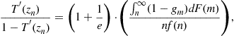 (17)
(17)
where ![]() is the social marginal welfare weight on individual
is the social marginal welfare weight on individual ![]() . This formula is derived in Diamond (1998).
. This formula is derived in Diamond (1998).
Under a linearized income tax system with marginal tax rate ![]() , we have
, we have ![]() and hence
and hence ![]() . Therefore, denoting by
. Therefore, denoting by ![]() the density of earnings at
the density of earnings at ![]() if the nonlinear tax were replaced by a linearized tax with marginal tax rate
if the nonlinear tax were replaced by a linearized tax with marginal tax rate ![]() , we have
, we have ![]() and hence
and hence ![]() . Therefore,
. Therefore, ![]() and we can rewrite Eq. (17) as
and we can rewrite Eq. (17) as
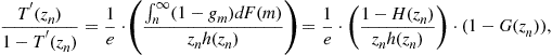 (18)
(18)
where ![]() is the average marginal social welfare weight on individuals above
is the average marginal social welfare weight on individuals above ![]() . Changing variables from
. Changing variables from ![]() to
to ![]() , we have
, we have ![]()
![]() where
where ![]() is the actual (not virtual) cumulative distribution of earnings. This establishes Eq. (11) in the main text. Note that the transversality condition implies that
is the actual (not virtual) cumulative distribution of earnings. This establishes Eq. (11) in the main text. Note that the transversality condition implies that ![]() .
.
Equation (17) is particularly easy to use for numerical simulations calibrated to the actual income distribution. Using the specified utility function ![]() , the distribution
, the distribution ![]() is calibrated so that, using the actual tax system, the resulting earnings distribution
is calibrated so that, using the actual tax system, the resulting earnings distribution ![]() match the actual earnings distribution. Once
match the actual earnings distribution. Once ![]() is obtained, formula (17) can be used iteratively until a fixed point tax system
is obtained, formula (17) can be used iteratively until a fixed point tax system ![]() is found. See e.g., Brewer et al. (2010) for an application to the UK case.
is found. See e.g., Brewer et al. (2010) for an application to the UK case.
A.2 Optimal Bottom Tax Rate in the Mirrlees Model
In the Mirrlees (1971) model, all individuals have the same utility function ![]() increasing in disposable income
increasing in disposable income ![]() and decreasing in labor supply
and decreasing in labor supply ![]() . Individuals differ only in their skill level, denoted by
. Individuals differ only in their skill level, denoted by ![]() , which measures their marginal productivity. Earnings are equal to
, which measures their marginal productivity. Earnings are equal to ![]() . The population is normalized to one and the distribution of skills is
. The population is normalized to one and the distribution of skills is ![]() , with density
, with density ![]() , and support
, and support ![]() . The government cannot observe skills and thus is restricted to setting taxes as a function only of earnings,
. The government cannot observe skills and thus is restricted to setting taxes as a function only of earnings, ![]() . Individual
. Individual ![]() chooses
chooses ![]() to maximize utility
to maximize utility ![]() leading to first order condition
leading to first order condition ![]() . Let
. Let ![]() , and
, and ![]() denote the consumption, earnings, and utility level of an individual with skill
denote the consumption, earnings, and utility level of an individual with skill ![]() . Note that
. Note that ![]() and
and ![]() .
.
To have a fraction of non-workers, we assume that ![]() for all
for all ![]() . As a result, all individuals with skill
. As a result, all individuals with skill ![]() below
below ![]() defined as
defined as ![]() will not work and choose the corner solution
will not work and choose the corner solution ![]() and
and ![]() . Hence, the fraction non-working in the population is
. Hence, the fraction non-working in the population is ![]() and naturally depends on both
and naturally depends on both ![]() (substitution effects) and
(substitution effects) and ![]() (income effects).
(income effects).
Using the envelope theorem, the utility ![]() of individual
of individual ![]() satisfies
satisfies ![]() . Note that this equation remains true even for non-workers at the bottom as
. Note that this equation remains true even for non-workers at the bottom as ![]() is constant with
is constant with ![]() and hence
and hence ![]() for
for ![]() .
.
The government maximizes a social welfare function,
![]()
Following Mirrlees (1971), in the maximization program of the government, ![]() is regarded as the state variable,
is regarded as the state variable, ![]() as the control variable, while
as the control variable, while ![]() is determined implicitly as a function of
is determined implicitly as a function of ![]() and
and ![]() from the equation
from the equation ![]() . The Hamiltonian is
. The Hamiltonian is
![]()
where ![]() is the multiplier of the state variable. As
is the multiplier of the state variable. As ![]() , the first order condition with respect to
, the first order condition with respect to ![]() is
is
![]()
At ![]() , and this first order condition becomes
, and this first order condition becomes
![]()
As ![]() , the first order condition with respect to
, the first order condition with respect to ![]() is
is
![]()
For ![]() are constant with
are constant with ![]() so that this equation simplifies to:
so that this equation simplifies to:
![]()
and can be integrated from ![]() to
to ![]() to yield
to yield
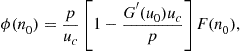
where we have used the transversality condition ![]() . Replacing this expression for
. Replacing this expression for ![]() into the first order condition for
into the first order condition for ![]() at
at ![]() yields
yields

which can be rewritten as
 (19)
(19)
where ![]() is the social marginal welfare weight on non-workers.116
is the social marginal welfare weight on non-workers.116
Recall that ![]() which defines
which defines ![]() . Hence, the substitution effect of
. Hence, the substitution effect of ![]() on
on ![]() (keeping
(keeping ![]() constant) is such that
constant) is such that ![]() . Hence, the elasticity of the fraction non-working
. Hence, the elasticity of the fraction non-working ![]() with respect to
with respect to ![]() is
is

which allows us to rewrite (19) as
![]()
exactly as in the discrete model formula (14) presented in the text.
Note that with quasi-linear iso-elastic preferences of the form ![]() , the individual first order condition is
, the individual first order condition is ![]() so that everybody with
so that everybody with ![]() works. If there is a positive fraction of individuals with zero skill (and hence not working), the formula above applies with
works. If there is a positive fraction of individuals with zero skill (and hence not working), the formula above applies with ![]() so that
so that ![]() . Intuitively, the fraction of individuals affected by a change in
. Intuitively, the fraction of individuals affected by a change in ![]() is negligible relative to the number of non-workers so that behavioral responses are negligible and hence
is negligible relative to the number of non-workers so that behavioral responses are negligible and hence ![]() .
.
References
1. Adema, W., Fron, P., & Ladaique, M. (2011). Is the European welfare state really more expensive? Indicators on social spending, 1980–2012; and a manual to the OECD social expenditure database. OECD social, employment and migration working papers, No. 124.
2. Ahmad E, Stern N. The theory of reform and Indian direct taxes. Journal of Public Economics. 1984;25:259–298.
3. Akerlof G. The economics of tagging as applied to the optimal income tax, welfare programs, and manpower planning. American Economic Review. 1978;68(1):8–19.
4. Alesina A, Giuliano P. Preferences for redistribution. In: Bisin AJ, Benhabib, eds. Handbook of Social Economics. Amsterdam: North Holland; 2011;93–132.
5. Alvaredo, F., Atkinson A., Piketty, T., & Saez, E. (2011). The World top incomes database. Online at <http://g-mond.parisschoolofeconomics.eu/topincomes/>.
6. Ardant G. Histoire de l’impôt. Vols. 1–2 Paris: Springer; 1971; p. 1971.
7. Atkinson A. Public economics in action. Oxford: Clarendon Press; 1995.
8. Atkinson, A. & Leigh, A. (2010). Understanding the distribution of top incomes in five Anglo-Saxon countries over the twentieth century. IZA discussion paper, No. 4937, May.
9. Atkinson A, Stiglitz JE. The design of tax structure: Direct versus indirect taxation. Journal of Public Economics. 1976;6(1–2):55–75.
10. Atkinson A, Stiglitz JE. Lectures in public economics. New York: McGraw Hill; 1980.
11. Atkinson A, Piketty T, Saez E. Top incomes in the long-run of history. Journal of Economic Literature. 2011;49(1):3–71.
12. Auerbach A. Capital gains taxation in the United States. Brookings Papers on Economic Activity. 1988;2:595–631.
13. Auerbach A, James H. Taxation and economic efficiency. In: 1st ed. Amsterdam: North-Holland; 2002;1347–1421. Auerbach A, Feldstein M, eds. Handbook of public economics. Vol. 3.
14. Bane MJ, Ellwood DT. Welfare realities: From rhetoric to reform. Cambridge: Harvard University Press; 1994.
15. Bebchuk L, Fried J. Pay without performance: The unfulfilled promise of executive compensation. Cambridge: Harvard University Press; 2004.
16. Bentham J. Principles of morals and legislation. London: Doubleday; 1791.
17. Besley T, Coate S. Workfare versus welfare: Incentives arguments for work requirements in poverty-alleviation programs. American Economic Review. 1992;82:249–261.
18. Best,M. & Kleven, H. 2012. Optimal income taxation with career effects of work effort. LSE working paper.
19. Blau F, Kahn L. Changes in the labor supply behavior of married women: 1980–2000. Journal of Labor Economics. 2007;25:393–438.
20. Blundell R, MaCurdy T. Labor supply: A review of alternative approaches. In: Amsterdam: North-Holland; 1999;Ashenfelter O, Card D, eds. Handbook of labor economics. Vol. 3.
21. Boadway R. From optimal tax theory to tax policy: Retrospective and prospective views, 2009 Munich lectures in economics. Cambridge, MA: MIT Press; 2012.
22. Boskin MJ, Sheshinski E. Optimal redistributive taxation when individual welfare depends upon relative income. Quarterly Journal of Economics. 1978;92(4):589–601.
23. Boskin MJ, Sheshinski E. Optimal tax treatment of the family: Married couples. Journal of Public Economics. 1983;20(3):281–297.
24. Bourguignon F, Spadaro A. Tax-benefit revealed social preferences. Journal of Economic Inequality. 2012;10(1):75–108.
25. Bovenberg AL, Goulder LH. Environmental taxation and regulation. In: 1st ed. Amsterdam: North-Holland; 2002;1471–1545. Auerbach A, Feldstein M, eds. Handbook of Public Economics. Vol. 3.
26. Brewer M, Saez E, Shephard. A. Means-testing and tax rates on earnings. In: Dimension of tax design: The mirrlees review institute for fiscal studies. Oxford University Press 2010;90–173.
27. Cagé, J., & Gadenne, L. (2012).The fiscal cost of trade liberalization. working paper, Harvard and PSE.
28. Card D, Mas A, Moretti E, Saez E. Inequality at work: The effect of peers salary on job satisfaction. American Economic Review. 2012;102(6):2981–3003.
29. Chetty R. A new method of estimating risk aversion. American Economic Review. 2006;96(5):1821–1834.
30. Chetty R. Moral hazard vs liquidity and optimal unemployment insurance. Journal of Political Economy. 2008;116(2):173–234.
31. Chetty R. Sufficient statistics for welfare analysis: A bridge between structural and reduced-form methods. Annual Review of Economics. 2009a;1:451–488.
32. Chetty R. Is the taxable income elasticity sufficient to calculate deadweight loss? The implications of evasion and avoidance. American Economic Journal: Economic Policy. 2009b;1(2):31–52.
33. Chetty R. Bounds on elasticities with optimization frictions: A synthesis of micro and macro evidence on labor supply. Econometrica. 2012;80(3):969–1018.
34. Chetty, R., Friedman, J., & Saez, E. forthcoming. Using differences in knowledge across neighborhoods to uncover the impacts of the EITC on earnings. NBER working paper, No. 18232. American Economic Review.
35. Chiappori P. Rational household labor supply. Econometrica. 1988;56(1):63–90.
36. Christiansen V, Tuomala M. On taxing capital income with income shifting. International Tax and Public Finance. 2008;15:527–545.
37. Congdon W, Mullainathan S, Schwartzstein J. A reduced form approach to behavioral public finance. Annual Review of Economics. 2012;4:511–540.
38. Crépon, B., Duflo, E., Gurgand, M., Rathelot, R. & Zamora, P. (in press). Do labor market policies have displacement effect? Evidence from a clustered randomized experiment. NBER working paper, No.18597. Quarterly Journal of Economics.
39. Cuff K. Optimality of workfare with heterogeneous preferences. Canadian Journal of Economics. 2000;33(1):149–174.
40. Currie J, Gahvari F. Transfers in cash and in-kind: Theory meets the data. Journal of Economic Literature. 2008;46(2):333–383.
41. Deaton A. Optimally uniform commodity taxes. Economic Letters. 1979;2:357–361.
42. Delalande, N. (2011a). Les Batailles de l’impôt. Consentement et résistances de 1789 à nos jours. Paris Seuil, coll. L’Univers historique.
43. Delalande N. La Réforme Fiscale et l’Invention des Classes Moyennes–l’Exemple de la Création de l’Impôt sur le Revenu. In: Bezes P, Siné A, eds. Gouverner (par) les Finances Publiques. Paris: Presses de Sciences Po; 2011b.
44. Diamond P. A many-person ramsey tax rule. Journal of Public Economics. 1975;4(4):335–342.
45. Diamond P. Income taxation with fixed hours of work. Journal of Public Economics. 1980;13:101–110.
46. Diamond P. Optimal income taxation: An example with a U-shaped pattern of optimal marginal tax rates. American Economic Review. 1998;88:83–95.
47. Diamond P, Mirrlees J. Optimal taxation and public production I: Production efficiency and II: Tax rules. American Economic Review. 1971;6:8–27 and 261–278.
48. Diamond, P. & Mirrlees, J. (Unpublished). Optimal Taxation and the Le Chatelier Principle. MIT working paper.
49. Diamond P, Saez E. The case for a progressive tax: From basic research to policy recommendations. Journal of Economic Perspectives. 2011;25(4):165–190.
50. Diamond P, Sheshinski E. Economic aspects of optimal disability benefits. Journal of Public Economics. 1995;57:1–23.
51. Duflo E. Grandmothers and granddaughters: Old-age pensions and intra-household allocation in South Africa. World Bank Economic Review. 2003;17:1–25.
52. Dupuit J. On the measurement of the utility of public works translated. In: Arrow KJ, Scitovsky T, eds. Readings in welfare economics (1969). London: Allen and Unwin; 1844.
53. Eaton J, Rosen HS. Optimal redistributive taxation and uncertainty. Quarterly Journal of Economics. 1980;95:357–364.
54. Edgeworth FY. The pure theory of taxation. Economic Journal. 1897;7:46–70 226–238, and 550–571.
55. Eurostat. Taxation trends in the European union. Luxembourg: Publications Office of the European Union; 2012.
56. Fehr E, Schmidt KM. A theory of fairness, competition, and cooperation. Quarterly Journal of Economics. 1999;114(3):817–868.
57. Feldstein M. The effect of marginal tax rates on taxable income: A panel study of the 1986 tax reform act. Journal of Political Economy. 1995;103(3):551–572.
58. Feldstein M. Tax avoidance and the deadweight loss of the income tax. Review of Economics and Statistics. 1999;81(4):674–680.
59. Feldstein M. The mirrlees review. Journal of Economic Literature. 2012;50(3):781–790.
60. Fisher I. Economists in public service: Annual address of the president. American Economic Review. 1919;9(1):5–21.
61. Fleurbaey M. On fair compensation. Theory and Decision. 2004;36:277–307.
62. Fleurbaey M. Fairness, Responsability and Welfare. Oxford: Oxford University Press; 2008.
63. Fleurbaey M, Maniquet F. A theory of fairness and social welfare. Cambridge: Cambridge University Press; 2011.
64. Flora P. State economy and society in western Europe. vol. I London: Macmillan Press; 1983; pp. 1815–1975.
65. Fong C. Social preferences, self-interest, and the demand for redistribution. Journal of Public Economics. 2001;82(2):225–246.
66. Frohlich N, Oppenheimer JA. Choosing justice: An experimental approach to ethical theory. Berkeley: Berkeley University of California Press, Berkeley University Press; 1992.
67. Gauthier AH. The impact of family policies on fertility in industrialized countries: A review of the literature. Population Research and Policy Review. 2007;26(3):323–346.
68. Golosov, Michael, Tsyvinski, Aleh, & Ivan Werning. 2006. New dynamic public finance: A user’s guide. NBER Macroeconomics Annual. volume 21, chapter 5, 317–385, Cambridge, MA: MIT Press.
69. Goolsbee A. What happens when you tax the rich? Evidence from executive compensation. Journal of Political Economy. 2000;108(2):352–378.
70. Gordon R, Slemrod J. Are real responses to taxes simply income shifting between corporate and personal tax bases? In: Slemrod J, ed. Does atlas shrug? The economic consequences of taxing the rich. New York: Russell Sage Foundation and Harvard University Press; 2000;240–288.
71. Guesnerie R. A contribution to the pure theory of taxation. Cambridge, MA: Cambridge University Press; 1995.
72. Hungerbuhler M, Lehmann E, Parmentier A, Der Linden V, Bruno. Optimal redistributive taxation in a search equilibrium model. Review of Economic Studies. 2006;73:743–767.
73. Kaplow L. On the undesirability of commodity taxation even when income taxation is not optimal. Journal of Public Economics. 2006;90(6–7):1235–1250.
74. Kaplow L. The theory of taxation and public economics. Princeton: Princeton University Press; 2008.
75. Katz MB. In the shadow of the poorhouse: A social history of welfare in the United States. 2nd ed New York, NY: Basic Books; 1996.
76. Kirchgassner G, Pommerehne W. Tax harmonization and tax competition in the European union: Lessons from Switzerland. Journal of Public Economics. 1996;60:351–371.
77. Kleven H, Kopczuk W. Transfer program complexity and the take up of social benefits. American Economic Journal: Economic Policy. 2011;3:54–90.
78. Kleven,H., & Schultz, E. (2012). Estimating taxable income responses using danish tax reforms. LSE working paper.
79. Kleven H, Kreiner C, Saez E. The optimal income taxation of couples. Econometrica. 2009a;77(2):537–560.
80. Kleven, H., Kreiner, C., & Saez, E. (2009b).Why can modern governments tax so much? An agency model of firms as fiscal intermediaries. NBER working paper, No. 15218.
81. Kleven, H., Landais, C., Saez, E., & Schultz, E. (2013). Migration and wage effects of taxing top earners: Evidence from the foreigners’ tax scheme in Denmark. NBER working paper, No. 18885.
82. Kleven, H., Landais, C., & Saez, E. (in press). Taxation and international mobility of superstars: Evidence from the European football market. American Economic Review.
83. Kocherlakota NR. The new dynamic public finance. Princeton: Princeton University Press; 2010.
84. Kolm S-C. Modern theories of justice. Cambridge: MIT Press; 1996.
85. Kopczuk W. Tax bases, Tax rates and the elasticity of reported income. Journal of Public Economics. 2005;89(11–12):2093–2119.
86. Landais, C., Michaillat, P., & Saez, E. (2010). Optimal unemployment insurance over the business cycle. NBER working paper, No. 16526.
87. Landais C, Piketty T, Saez E. Pour une révolution fiscale: Un impôt sur le revenu pour le XXIème siècle. Paris: Le Seuil; 2011.
88. Laroque GR. Indirect taxation is superfluous under separability and taste homogeneity: A simple proof. Economics Letters. 2005;87(1):141–144.
89. Lee D, Saez E. Optimal minimum wage in competitive labor markets. Journal of Public Economics. 2012;96(9–10):739–749.
90. Lindert P. Growing public: Social spending and economic growth since the eighteenth century. Two volumes Cambridge, MA: Cambridge University Press; 2004.
91. Lochner L, Monge-Naranjo A. The nature of credit constraints and human capital. American Economic Review. 2011;101(6):2487–2529.
92. Lockwood, B. B., & Weinzierl, M. C. 2012. De Gustibus non est taxandum: Theory and evidence on preference heterogeneity and redistribution. NBER working paper, No. 17784.
93. Lundberg S, Pollak R, Wales T. Do husbands and wives pool their resources? Evidence from the United Kingdom child benefit. Journal of Human Resources. 1997;32:463–480.
94. Luttmer E. Neighbors as negatives: Relative earnings and well-being. Quarterly Journal of Economics. 2005;120(3):963–1002.
95. Mankiw NG, Weinzierl M. The optimal taxation of height: A case study of utilitarian income redistribution. American Economic Journal: Economic Policy. 2010;2(1):155–176.
96. Mehrotra, A.K. (2005). Edwin R.A. Seligman and the beginnings of the US income tax. Tax Notes (pp. 933–950) [November 14].
97. Mirrlees JA. An exploration in the theory of optimal income taxation. Review of Economic Studies. 1971;38:175–208.
98. Mirrlees JA. Optimal tax theory: A synthesis. Journal of Public Economics. 1976;6:327–358.
99. Mirrlees JA. Migration and optimal income taxes. Journal of Public Economics. 1982;18:319–341.
100. Mirrlees JA. The theory of optimal taxation. In: Amsterdam: North-Holland; 1986;1197–1249. Arrow KJ, Intriligator MD, eds. Handbook of mathematical economics. Vol. 3.
101. Mirrlees JA, ed. Dimension of tax design: The mirrlees review. Institute for Fiscal Studies, Oxford: Oxford University Press; 2010.
102. Mirrlees JA, ed. Tax by design: The mirrlees review. Institute for Fiscal Studies, Oxford: Oxford University Press; 2011.
103. Moffitt R, Wilhelm M. Taxation and the labor supply decisions of the affluent. In: Slemrod J, ed. Does atlas shrug? The economic consequences of taxing the rich. New York: Russell Sage Foundation and Harvard University Press; 2000;193–234.
104. Musgrave R. A brief history of fiscal doctrine. In: Amsterdam: North-Holland; 1985;1–59. Auerbach AJ, Feldstein M, eds. Handbook of Public Economics. Vol. 1.
105. Naito H. Re-examination of uniform commodity taxes under a non-linear income tax system and its implication for production efficiency. Journal of Public Economics. 1999;71:165–188.
106. Nichols A, Zeckhauser R. Targeting transfers through restrictions on recipients. American Economic Review. 1982;72(2):372–377.
107. OECD. Personal income tax systems. Paris: OECD; 1986.
108. OECD. (2005). Increasing financial incentives to work: The role of in-work benefits. In OECD employment outlook, OECD, Paris [2005 Edition].
109. OECD. (2006). Policies targeted at specific workforce groups or labour market segments. In OECD employment outlook: Boosting jobs and incomes, OECD, Paris [2006 Edition].
110. OECD. (2011a). Revenue statistics, 1965–2010. OECD, Paris [2011 Edition].
111. OECD. (2011b). The taxation of low-income workers. In OECD tax policy study No. 21: Taxation and employment, OECD, Paris.
112. OECD. (2011c). The taxation of mobile high-skilled workers. In OECD Tax Policy Study No. 21: Taxation and employment, OECD, Paris.
113. Oswald AJ. Altruism, jealousy and the theory of optimal non-linear taxation. Journal of Public Economics. 1983;20(1):77–87.
114. Pareto, V. 1896. La courbe de la répartition de la richesse. Ecrits sur la courbe de la répartition de la richesse (pp. 1–15) [Writings by Pareto collected by G. Busino, Librairie Droz, 1965].
115. Persson T, Tabellini G. Political economics and public finance. In: Amsterdam: North-Holland; 2002;991–1042. Auerbach AJ, Feldstein M, eds. Handbook of public economics. Vol. 3.
116. Piketty T. Social mobility and redistributive politics. Quarterly Journal of Economics. 1995;110(3):551–584.
117. Piketty T. La redistribution fiscale face au Chômage. Revue Française d’Economie. 1997;12:157–201.
118. Piketty T. Les hauts revenus en France au 20e siècle—Inégalités et redistributions 1901–1998. Paris: Grasset; 2001; p. 807.
119. Piketty T, Nancy Q. Income inequality and progressive income taxation in China and India: 1986–2015. American Economic Journal Applied Economics. 2009;1(2):53–63.
120. Piketty T, Saez E. Income inequality in the United States, 1913–1998. Quarterly Journal of Economics. 2003;118(1):1–39.
121. Piketty T, Saez E. How progressive is the US federal tax system? A historical and international perspective. Journal of Economic Perspectives. 2007;21(1):3–24.
122. Piketty, T., & Saez, E. (2012a). A theory of optimal capital taxation. NBER Working Paper, No. 17989.
123. Piketty, T., & Saez, E. (forthcoming). A theory of optimal inheritance taxation. CEPR discussion paper, No. 9241. Econometrica.
124. Piketty, T., Saez, E., & Stantcheva, S. (forthcoming). Optimal taxation of top labor incomes: A tale of three elasticities. NBER working paper. No. 17616. American Economic Journal: Economic Policy.
125. Ramey VA, Francis N. A century of work and leisure. American Economic Journal: Macroeconomics. 2009;1(2):189–224.
126. Ramsey F. A contribution to the theory of taxation. Economic Journal. 1927;37(145):47–61.
127. Roemer J. Equality of opportunity. Cambridge: Harvard University Press; 1998.
128. Roemer J, et al. To what extent do fiscal systems equalize opportunities for income acquisition among citizens? Journal of Public Economics. 2003;87:539–565.
129. Roine J, Vlachos J, Waldenstrom D. The long-run determinants of inequality: what can we learn from top income data? Journal of Public Economics. 2009;93(7–8):974–988.
130. Rothschild, C., & Scheuer, F. (2011). Optimal taxation with rent-seeking. NBER working paper, No. 17035.
131. Sadka E. On income distribution, incentive effects and optimal income taxation. Review of Economic Studies. 1976;43(1):261–268.
132. Saez, E. 1999. A characterization of the income tax schedule minimizing deadweight burden. MIT PhD thesis.
133. Saez E. Using elasticities to derive optimal income tax rates. Review of Economic Studies. 2001;68:205–229.
134. Saez E. Optimal income transfer programs: Intensive versus extensive labour supply responses. Quarterly Journal of Economics. 2002a;117(2):1039–1073.
135. Saez E. The desirability of commodity taxation under non-linear income taxation and heterogeneous tastes. Journal of Public Economics. 2002b;83(2):217–230.
136. Saez E. The optimal treatment of tax expenditures. Journal of Public Economics. 2004a;88(12):2657–2684.
137. Saez E. Direct or indirect tax instruments for redistribution: Short-run versus long-run. Journal of Public Economics. 2004b;88(3–4):503–518.
138. Saez, E. (2004c). Reported incomes and marginal tax rates, 1960–2000: Evidence and policy implications. In J. Poterba (Ed.), Tax policy and the economy. Vol. 18 (pp. 117–174).
139. Saez, E. & Stantcheva, S. (2013). Generalized social marginal welfare weights for optimal tax theory. NBER working paper, No. 18835.
140. Saez E, Slemrod J, Giertz S. The elasticity of taxable income with respect to marginal tax rates: A critical review. Journal of Economic Literature. 2012;50(1):3–50.
141. Seade JK. On the shape of optimal tax schedules. Journal of Public Economics. 1977;7(1):203–236.
142. Seade JK. On the sign of the optimum marginal income tax. Review of Economic Studies. 1982;49:637–643.
143. Seligman ERA. The income tax: A study of the history, theory and practice of income taxation at home and abroad. New York: Macmillan; 1911.
144. Sheshinski E. The optimal linear income tax. Review of Economic Studies. 1972;39(3):297–302.
145. Simula L, Trannoy A. Optimal income tax under the threat of migration by top-income earners. Journal of Public Economics. 2010;94:163–173.
146. Slemrod J. High income families and the tax changes of the 1980s: The anatomy of behavioral response. In: Feldstein M, Poterba J, eds. Empirical foundations of household taxation. Chicago: University of Chicago Press; 1996;169–192.
147. Slemrod J, Kopczuk W. The optimal elasticity of taxable income. Journal of Public Economics. 2002;84(1):91–112.
148. Slemrod J, Yitzhaki S. Tax avoidance, evasion and administration. In: 1st ed. Amsterdam: North-Holland; 2002;1423–1470. Auerbach A, Feldstein M, eds. Handbook of public economics. Vol. 3.
149. Sorensen PB. Optimal tax progressivity in imperfect labour markets. Labour Economics. 1999;6:435–452.
150. Stantcheva S. Optimal taxation with adverse selection in the labor market. MIT working paper 2011.
151. Stiglitz J. Self-selection and Pareto efficient taxation. Journal of public economics. 1982;17:213–240.
152. Stiglitz J. Pareto efficient and optimal taxation and the new new welfare economics. In: Amsterdam: North-Holland; 1987;991–1042. Auerbach AJ, Feldstein M, eds. Handbook of Public Economics. Vol. 2.
153. Treasury US. Simple, fair, and pro-growth: Proposals to fix America’s tax system. Washington, DC: President’s Advisory Panel on Federal Tax Reform; 2005.
154. Tuomala M. Optimal income tax and redistribution. Oxford: Clarendon Press; 1990.
155. US Treasury Department, Internal Revenue Service. (2012). Statistics of income: Individual statistical tables by tax rate and income percentile. Table 1 available online at http://www.irs.gov/taxstats/indtaxstats/article/0,id=133521,00.html.
156. Varian HR. Redistributive taxation as social insurance. Journal of Public Economics. 1980;14(1):49–68.
157. Vickrey W. Measuring marginal utility by reactions to risk. Econometrica. 1945;13:319–333.
158. Webber C, Wildavsky AB. A history of taxation and expenditure in the western world. New York: Simon and Schuster; 1986.
159. Weinzierl MC. The surprising power of age-dependent taxes. Review of Economic Studies. 2011;78(4):1490–1518.
160. Weinzierl, M. C. (2012).Why do we redistribute so much but tag so little? The principle of equal sacrifice and optimal taxation. Harvard business school working paper, No: 12-64.
161. Werning, I. (2007). Pareto efficient income taxation. MIT working paper.
162. Wilson RB. Nonlinear pricing. Oxford: Oxford University Press; 1993.
163. Young C, Varner C. Millionaire migration and state taxation of top incomes: Evidence from a natural experiment. National Tax Journal. 2011;64:255–284.
1Boadway (2012) also provides a recent, longer, and broader survey that aims at connecting theory to practice.
2The analysis of optimal capital income taxation naturally involves dynamic considerations and is covered in the chapter by Kopczuk in this volume.
3Naturally, the set of possible tax systems evolves overtime with technological progress. If more complex tax innovations become feasible and can realistically generate large welfare gains, they are certainly worth considering.
4The simple tax structure approach also helps with conditions (1) and (2) as the economic trade-offs are simpler and more transparent, and the formulas for simple tax structures tend to easily generalize to heterogeneous populations.
5See Golosov, Tsyvinski, and Werning (2006) and Kocherlakota (2010) for recent surveys of the new dynamic public finance literature. Piketty and Saez (2012a,b) analyze the problem optimal taxation of capital and inheritances in a dynamic model but using a sufficient statistics approach and focusing on simple tax structures.
6This is defining taxes on capital as the sum of property and wealth taxes, inheritance and gift taxes, taxes of corporate and business profits, individual income taxes on individual capital income, and the share of consumption taxes falling on capital income. Naturally, there are important variations over time and across countries in the relative importance of these various capital tax instruments. See e.g., Piketty and Saez (2012a).
7Including payroll taxes, individual income tax on labor income, and the share of consumption taxes falling on labor income.
8Again, there are important variations in capital taxes which fall beyond the scope of this chapter. In particular, corporate tax rates have declined significantly in Europe since the early 1990s (due to tax competition), but tax revenues have dropped only slightly, due to a global rise in the capital share, the causes of which are still debated. See e.g., Eurostat (2012).
9See e.g., Piketty and Qian (2009) for a contrast between China (where the income tax is about to become a mass tax, like in developed countries) and India (where the income tax is still very much an elite tax raising limited revenue). Cagé and Gadenne (2012) provide a comprehensive empirical analysis of the extent to which low- and middle-income countries were able to replace declining trade tax revenues by modern broad based taxes since the 1970s. See Kleven, Kreiner and Saez (2009b) for a theoretical model of the fiscal modernization process.
10For example, (Landais, Piketty, and Saez (2011)) show that tax rates decline at the very top of the French income distribution because of such preferential tax treatment and of various tax loopholes and fiscal optimization strategies. In the United States as well, income tax rates decline at the very top due to the preferential treatment of realized capital gains which constitute a large fraction of top incomes (US Treasury, 2012). See Piketty and Saez (2007) for an analysis of progressivity of the federal tax system since 1960. Note that preferential treatment for capital income did not exist when modern income taxes were created in 1900–1920. Preferential treatment was developed mostly in the postwar period in order to favor savings and reconstruction, and then extended since the 1980–1990s in the context of financial globalization and tax competition. For a detailed history in the case of France, see Piketty (2001).
11See Atkinson, Piketty and Saez (2011) for a recent survey. One of the main findings of this literature is that the historical decline in top income shares that occurred in most countries during the first half of the twentieth century has little to do with a Kuznets-type process. It was largely due to the fall of top capital incomes, which apparently never fully recovered from the 1914–1945 shocks, possibly because of the rise of progressive income and estate taxes and their dynamic impact of savings, capital accumulation and wealth concentration.
12Family benefits can also be considered as part of education spending. Note that the boundaries between the various social spending categories reported on Table 1 are not entirely homogenous across OECD countries (e.g., family benefits are split between “Income support to the working age” and “Other social public spending”). Also differences in tax treatment of transfers further complicate cross country comparisons. Here we simply care about the broad orders of magnitude. For a detailed cross-country analysis, see Adema, Fron, and Ladaique (2011).
13Naturally, higher income individuals are often better able to navigate the public education and health care systems and hence tend to get a better value out of those benefits than lower income individuals. However, the value of those benefits certainly grows less than proportionally to income.
14In most countries, benefits are proportional to payroll tax contributions. Some countries—such as the United Kingdom—provide a minimum pension that is closer to a demogrant.
15It should be noted that the motivation behind the historical rise of these public services has to do not only with redistributive objectives, but also with the perceived failure of competitive markets in these areas (e.g., regarding the provision of health insurance or education). We discuss issues of individual and market failures in Section 6 below.
16Note that this graph ignores important elements. First, the health insurance Medicaid program in the United States is means-tested and adds a significant layer of implicit taxation on low income work. France offers universal health insurance which does not create any additional implicit tax on work. Second, the graph ignores in-kind benefits for children such as subsidized child care and free pre-school kindergarten in France that have significant value for working single parents. Such programs barely exist in the United States. Third, the graph ignores housing benefits, which are substantial in France. Fourth, the graph ignores temporary unemployment insurance benefits which depend on previous earnings for those who have become recently unemployed and which are significantly more generous in France both in level and duration. Finally, this graph ignores consumption taxes, implying that the cutoff income level below which transfers exceed taxes is significantly overestimated. This cutoff also greatly varies with the family structure (e.g., able bodied single individuals with no dependent receive zero cash transfers in the US but significant transfers in France).
17See e.g., Mehrotra (2005) for a longer discussion of the role of Seligman on US tax policy at the beginning of the 20th century.
18This is particularly true in countries like France where mainstream laissez-faire economists had little sympathy for Anglo-Saxon utilitarian arguments, and were originally very hostile to tax progressivity, which they associated with radical utopia and with the French Revolution. See e.g., Delalande (2011a,b, pp. 166-170).
19Boadway (2012), Chapter 1 provides a longer discussion of the role played by such reviews.
20For a survey of historical fiscal doctrine in general see Musgrave (1985, chap. 1). For a more complete overview of modern optimal Boadway (2012), chapter 2.
21Vickrey (1945) had proposed an earlier formalization of the problem but without solving explicitly for optimal tax formulas.
22Stiglitz (1987, chap. 15) handbook chapter on optimal taxation provides a comprehensive optimal tax survey using the Stiglitz (1982) discrete model. In this chapter, we will not use the Stiglitz (1982) discrete model and present instead an alternative discrete model, first developed by Piketty (1997) which generates optimal tax formulas very close to those of the continuous model, and much easier to calibrate meaningfully.
23In the field of nonlinear pricing in industrial organization, the use of elasticity-based formulas came earlier (see e.g., Wilson, 1993).
24Utilitarianism as a social justice criterion was developed by the English philosopher Bentham in the late 18th century (Bentham, 1791).
25Naturally, the two concepts are not independent. If individuals have very concave utilities, they will naturally support more redistribution under the “veil of ignorance,” and the government choice for ![]() will reflect those views.
will reflect those views.
26As we saw, under utilitarianism and concave and uniform utility functions across individuals, this implies complete equalization of post-tax incomes.
27In the model above, the government would impose taxes ![]() based on the intrinsic characteristics of individual
based on the intrinsic characteristics of individual ![]() but independent of the behavior of individual
but independent of the behavior of individual ![]() so as to equalize all the
so as to equalize all the ![]() ’s across individuals (in the equilibrium where each individual chooses labor supply optimally given
’s across individuals (in the equilibrium where each individual chooses labor supply optimally given ![]() ).
).
28When incomes were not observable, archaic tax systems did rely on quasi-exogenous characteristics such as nobility titles, or land taxes based on rarely updated cadasters (Ardant, 1971). Ironically, when incomes become observable, such quasi-first best taxes were replaced by second-best income-based taxes.
29As mentioned above, the set of tools available changes over time. For example, individual incomes become observable only in modern economies.
30Formally ![]() solves the problem
solves the problem ![]() subject to
subject to ![]() .
.
31In terms of informational constraints, the government would be constrained to use linear taxation (instead of the more general nonlinear taxation) if it can only observe the amount of each earnings transaction but cannot observe the identity of individual earners. This could happen for example if the government can only observe the total payroll paid by each employer but cannot observe individual earnings perhaps because there is no identity number system for individuals.
32To see this, recall that ![]() so that
so that ![]() .
.
33It is not exactly a compensated elasticity as ![]() is income weighted while
is income weighted while ![]() is not.
is not.
34This assumes that a lump sum tax ![]() is feasible to fund government spending. If lump sum taxes are not feasible, for example because it is impossible to set taxes higher than earnings at the bottom, then the optimal tax in that case is the smallest
is feasible to fund government spending. If lump sum taxes are not feasible, for example because it is impossible to set taxes higher than earnings at the bottom, then the optimal tax in that case is the smallest ![]() such that
such that ![]() , i.e., the level of tax required to fund government spending
, i.e., the level of tax required to fund government spending ![]() .
.
35Naturally, such long-run responses are challenging to estimate empirically as short-term comparisons around a tax reform cannot capture them.
36Varian (1980) analyzes the optimal nonlinear tax with random earnings.
37To see this, if the alternative is ![]() , everybody below and including the median prefers
, everybody below and including the median prefers ![]() to
to ![]() so that
so that ![]() wins. Conversely, if
wins. Conversely, if ![]() , everybody above and including the median prefers
, everybody above and including the median prefers ![]() to
to ![]() and
and ![]() still wins.
still wins.
38Formula (4) shows that if ![]() , then a negative tax rate is actually optimal. Empirically however, it is always the case that
, then a negative tax rate is actually optimal. Empirically however, it is always the case that ![]() .
.
39Note however that the tax base tends to be smaller than national income as some forms of income (or consumption) are excluded from the tax base. Therefore, with existing tax bases, the tax rate needed to raise say 40% of national income, will typically be somewhat higher, perhaps around 50%.
40![]() is endogenously determined using the actual US earnings distribution and assuming that government required spending
is endogenously determined using the actual US earnings distribution and assuming that government required spending ![]() (outside transfers) is 10% of total actual earnings. The distribution is for earnings of individuals aged 25 to 64 from the 2011 Current Population Survey for 2010 earnings.
(outside transfers) is 10% of total actual earnings. The distribution is for earnings of individuals aged 25 to 64 from the 2011 Current Population Survey for 2010 earnings.
41Examples of such avoidance/evasion are (a) reductions in current cash compensation for increased fringe benefits or deferred compensation such as stock-options or future pensions, (b) increased consumption within the firm such as better offices, vacation disguised as business travel, private use of corporate jets, etc., (c) re-characterization of ordinary income into tax favored capital income, and (d) outright tax evasion such as using off-shore accounts.
42Slemrod and Kopczuk (2002) endogenize avoidance opportunities in a multi-good model where the government selects the tax base. Finally, a large literature (surveyed in Slemrod and Yitzhaki (2002)) analyzes optimal policy design in the presence of tax evasion.
43Kopczuk (2005) shows that the Tax Reform Act of 1986 in the United States, which broadened the tax base and closed loopholes did reduce the elasticity of reported income with respect to the net-of-tax rate.
44Offshore tax evasion is very difficult to fight from a single country’s perspective but can be overcome with international coordination. This shows again that whether a tax avoidance/evasion opportunity can be eliminated depends on the institutional framework.
45Slemrod and Kopczuk (2002) present a model with costs of enforcement, where the government can adopt a broader tax base but where expanding the tax base is costly, to capture this trade-off theoretically.
46Other examples could be individual income vs. corporate income, or realized capital gains vs. ordinary income, or self-employment earnings vs. employee earnings.
47Chiappori (2008) propose an optimal tax analysis with shifting between capital and labor income in an OLG model.
48This model nests the pure tax avoidance model of the previous section in the case where ![]() , i.e., there is no intrinsic capital income.
, i.e., there is no intrinsic capital income.
49As we have no income effects, the elasticities are also compensated elasticities.
50Note that there also exists dynamic reasons—e.g., the relative importance of inheritance and life-cycle saving in aggregate wealth accumulation—explaining why one might want to tax capital income more than labor income. See Piketty and Saez (2012a).
51The optimal income tax theory following Mirrlees (1971) has devoted substantial effort studying those issues thoroughly (see e.g., Mirrlees (1976,1986, chap. 24) for extensive surveys). The formal derivations are gathered in the appendix.
52Because the individual chooses ![]() to maximize utility, the money-metric welfare effect of the reform on individual
to maximize utility, the money-metric welfare effect of the reform on individual ![]() is given by
is given by ![]() using the standard envelope theorem argument (see the end of Section 3.3).
using the standard envelope theorem argument (see the end of Section 3.3).
53Note that the derivation and formula are virtually the same as for the optimal linear rate by simply multiplying ![]() by the factor
by the factor ![]() . Indeed, when
. Indeed, when ![]() and the problem boils down to the optimal linear tax problem.
and the problem boils down to the optimal linear tax problem.
54Saez (2001) provides a decomposition and shows that ![]() with
with ![]() the average (income weighted) uncompensated elasticity and
the average (income weighted) uncompensated elasticity and ![]() the (unweighted) average income effect.
the (unweighted) average income effect.
55This graph is taken from Diamond and Saez (2011) who use the 2005 distribution of total pre-tax family income (including capital income and realized capital gains) based on tax return data.
56A Pareto distribution with parameter ![]() has a distribution of the form
has a distribution of the form ![]() and density
and density ![]() (with
(with ![]() a constant parameter). For any
a constant parameter). For any ![]() , the average income above
, the average income above ![]() is equal to
is equal to ![]() .
.
57In principle, executives could also be underpaid relative to their marginal product if there is social outrage about high levels of compensation. In that case, a company might find it more profitable to under-pay its executives than face the wrath of its other employees, customers, or the public in general.
58A few studies have analyzed optimal taxation in models with labor market imperfections such as search models, union models, efficiency wages models (see Sorensen, 1999 for a survey). Few papers have addressed redistributive optimal tax policy in models with imperfect labor markets. Hungerbuhler, Lehmann, Parmentier Der Linden, and Bruno (2006) analyze a search model with heterogeneous productivity, and Stantcheva (2011) considers contracting models where firms cannot observe perfectly the productivity of their employees.
59In their model (and in contrast to the simple model we use here), when rent-seekers “steal” only from other rent-seekers, it is not optimal to impose high top tax rates because low top tax rates stimulate rent-seeking efforts, thereby congesting the rent-seeking sector and discouraging further entry.
60Piketty et al. (2011) show that this assumption can be relaxed without affecting the substance of the results.
61The same issue arises with optimal Ramsey taxation in the presence of imperfect competition, which has been explored in depth in the traditional optimal tax literature (see e.g., Auerbach and James (2002), Section 7 for a survey).
62The government can use other tools, such as immigration policy, to affect migration. Those other tools are taken here as given. Note that democracies typically do not control emigration but can control to some extent immigration. In the European Union context, emigration and immigration across EU countries is almost completely deregulated and hence our analysis is relevant in this context.
63Simula and Trannoy (2010) also derive optimal income tax formulas in a model including both migration and standard labor supply responses.
64E.g. the Mirrlees Report is sometimes ambiguous as to whether the objective is to maximize social welfare at the global level or to find the tax system maximizing UK welfare.
65For example, the US Tax Reform Act of 1986 which cut the top marginal tax rate from 50% down to 28% led to a surge in reported top incomes but no effect on hours of work of top income earners (Moffitt & Wilhelm, 2000).
66For example, Slemrod (1996), Gordon and Slemrod (2000), and Saez (2004c) showed that part of the surge in top incomes immediately following the US tax cuts of the 1980s was due to income shifting from the corporate toward the individual sector.
67Auerbach (1988) showed that realized capital gains surged in 1986, in anticipation of the increase in the tax rate on realized capital gains starting in 1987. Goolsbee (2000) showed that stock-option realizations surged in 1992, in anticipation of the 1993 increase in top tax rates.
68For example, Kleven and Schultz (2012) provide very compelling estimates of modest—but not zero—elasticities around large tax reforms in Denmark, where the tax system offers few avoidance opportunities.
69For example, most of the objections in the popular and political debate to the recently proposed top marginal income tax rate of 75% in France are centered around mobility concerns: Will top talented workers (and top fortunes) leave France?
70See Kirchgassner and Pommerehne (1996) on mobility across Swiss Cantons in response to Canton taxes or Young and Varner (2011) on mobility across US states in response to state income taxes.
71Analyzing the data in first differences can alleviate omitted variable bias but can only capture short-term effects of tax rates on top incomes, which might differ from long-term effects.
72When individual top tax rates are high (relative to corporate and realized capital gains tax rates), it becomes more advantageous for upper incomes to organize their business activity using the corporate form and retain profits in the corporation. Profits only show up on individual returns as realized capital gains when the corporate stock is eventually sold (see Gordon and Slemrod, 2000 for a detailed empirical analysis).
73If top income share variations were due solely to tax avoidance, taxable income subject to the progressive tax schedule should be much more elastic than a broader income definition that also includes forms of income that are tax favored. Indeed, in the pure tax avoidance scenario, total real income of top earners should be completely inelastic to tax rates.
74Piketty et al. (2011) provide suggestive micro-level evidence. They show that CEO pay sensitivity to outcomes outside CEOs’ control (such as industry wide shocks) is higher when top rates are low, both in the US time series and across countries.
75Atkinson (1995) and Diamond (1998) showed that this case generates simpler formulas. Saez (2001) considers the case with income effects.
76This derivation has ignored the fact that the tax schedule is locally nonlinear. Saez (2001) shows that, in the exact formula for ![]() , the density
, the density ![]() should be replaced by the “virtual density”
should be replaced by the “virtual density” ![]() defined as the density at
defined as the density at ![]() that would arise if the nonlinear tax system were replaced by the linearized tax system at point
that would arise if the nonlinear tax system were replaced by the linearized tax system at point ![]() (see the appendix for a formal treatment).
(see the appendix for a formal treatment).
77We call ![]() a local Pareto parameter because for an exact Pareto distribution,
a local Pareto parameter because for an exact Pareto distribution, ![]() is constant and equal to the Pareto parameter
is constant and equal to the Pareto parameter ![]() .
.
78This point does not seem to have been formally established in the case of optimal tax theory but is well known in the mathematically equivalent optimal nonlinear pricing problem in the Industrial Organization literature (see e.g., Wilson, 1993, Section 8.4).
79![]() is never optimal in the Mirrlees model when marginal welfare weights decrease with
is never optimal in the Mirrlees model when marginal welfare weights decrease with ![]() . This is because increasing
. This is because increasing ![]() locally (as depicted on Figure 6) would raise more revenue from everybody above
locally (as depicted on Figure 6) would raise more revenue from everybody above ![]() which is desirable for redistribution. The behavioral response
which is desirable for redistribution. The behavioral response ![]() in the small band would further increase tax revenue (as
in the small band would further increase tax revenue (as ![]() ) making the reform desirable.
) making the reform desirable.
80Income effects positively affect labor supply above ![]() so that the mechanical tax revenue increase is actually higher than
so that the mechanical tax revenue increase is actually higher than ![]() and the optimal tax rate is correspondingly higher (see Saez, 2001).
and the optimal tax rate is correspondingly higher (see Saez, 2001).
81When obtaining (12), it is important to note that, because of the envelope theorem, the effect of an infinitesimal change in ![]() has no discrete effect on welfare for individuals moving in or out of occupation
has no discrete effect on welfare for individuals moving in or out of occupation ![]() . Hence, the welfare effects on movers is second order. See Saez (2002a), appendix for complete details.
. Hence, the welfare effects on movers is second order. See Saez (2002a), appendix for complete details.
82Those preferences are embodied in the individual utility functions ![]() . In the case just described, we would have
. In the case just described, we would have ![]() with
with ![]() cost of effort to get job
cost of effort to get job ![]() , and
, and ![]() if
if ![]() .
.
83This result can be seen as the symmetric counterpart of the zero-top result. At the top, it is straightforward to show that the optimum marginal tax rate cannot be positive (if it were, set it to zero above ![]() , the top earner works more, is better off, and pays the same taxes). However, it is not as easy to show that the top rate cannot be negative (this requires the more sophisticated argument presented in comments of formula (11)). At the bottom symmetrically, it is straightforward to show that the optimum marginal tax rate cannot be negative (if it were, set it to zero below
, the top earner works more, is better off, and pays the same taxes). However, it is not as easy to show that the top rate cannot be negative (this requires the more sophisticated argument presented in comments of formula (11)). At the bottom symmetrically, it is straightforward to show that the optimum marginal tax rate cannot be negative (if it were, set it to zero below ![]() , the bottom earner works less, is better off, and pays the same taxes). However, it is not as easy to show that the bottom rate cannot be positive (this again requires a symmetric argument to the one presented in comments of formula (11).)
, the bottom earner works less, is better off, and pays the same taxes). However, it is not as easy to show that the bottom rate cannot be positive (this again requires a symmetric argument to the one presented in comments of formula (11).)
84This elasticity ![]() reflects substitution effects only, as income effects are second order when the marginal tax rate is changed only on a small band of income at the bottom.
reflects substitution effects only, as income effects are second order when the marginal tax rate is changed only on a small band of income at the bottom.
85It can be obtained from Eq. (13) noting that the average social marginal welfare weight is equal to one so that ![]() . Therefore,
. Therefore, ![]() . Finally, note that
. Finally, note that ![]() .
.
86In the Rawlsian case, ![]() and the optimum phase-out rate is almost 100% when the fraction non-working
and the optimum phase-out rate is almost 100% when the fraction non-working ![]() is small.
is small.
87Chetty (2012) argues that intensive elasticities are more affected by frictions or inattention issues than extensive elasticities. This makes it more challenging to identify long-run intensive elasticities. For example, Chetty, Friedman, and Saez (2012) show that intensive responses to the EITC can also be substantial in the long-run in places where knowledge about the EITC is high.
88At the optimum, it is always the case that ![]() so that the denominator in formula (16) is always positive. To see this, suppose
so that the denominator in formula (16) is always positive. To see this, suppose ![]() , then
, then ![]() as
as ![]() , implying that the reform
, implying that the reform ![]() described above is always welfare improving. This result can be understood as follows. Suppose we start from an initial tax system (not optimal) where
described above is always welfare improving. This result can be understood as follows. Suppose we start from an initial tax system (not optimal) where ![]() , i.e., low-skilled workers are deserving and their elasticity
, i.e., low-skilled workers are deserving and their elasticity ![]() is not too high. In such a configuration, it is always desirable to increase in-work benefits for low-skilled workers. Increasing in-work benefits reduces
is not too high. In such a configuration, it is always desirable to increase in-work benefits for low-skilled workers. Increasing in-work benefits reduces ![]() as low-skilled workers become less and less in need of additional support. At the optimum where (16) holds,
as low-skilled workers become less and less in need of additional support. At the optimum where (16) holds, ![]() . In the extreme case with no behavioral responses,
. In the extreme case with no behavioral responses, ![]() should be set so that
should be set so that ![]() . Conversely, when the elasticity
. Conversely, when the elasticity ![]() is very large, the optimal bottom tax rate goes to zero.
is very large, the optimal bottom tax rate goes to zero.
89See OECD (2005, chap. 3) for a review of all the in-work benefits introduced in OECD countries up to year 2004.
90See OECD 2011b for a summary of such payroll tax reductions in OECD countries.
91A good example would be disability status that can only be imperfectly observed and that individuals can fake to some extent.
92Note that this derivation assumes that labor supply choices ![]() are independent of
are independent of ![]() . This assumption is reasonable when
. This assumption is reasonable when ![]() is manipulated through cheating only but would not necessarily hold if
is manipulated through cheating only but would not necessarily hold if ![]() was manipulated through real choices (e.g., hurting oneself to becoming truly disabled).
was manipulated through real choices (e.g., hurting oneself to becoming truly disabled).
93Traditionally, excise taxes have been used on goods where transactions were relatively easy for the government to monitor. In modern times, current excise taxes are often justified because of externalities (e.g., gasoline taxes because of pollution or global warming), or “internalities” (e.g., tobacco and addiction in models with self-control issues). We assume away such effects in what follows. Externalities are covered in the handbook chapter by Bovenberg and Goulder (2002).
94The Laroque-Kaplow method can be easily adapted to the linear earnings tax case. Consider a linear earnings tax with tax rate ![]() and demogrant
and demogrant ![]() . The same proof carries over if any tax system
. The same proof carries over if any tax system ![]() can be replaced by a pure income tax
can be replaced by a pure income tax ![]() such that
such that ![]() for all
for all ![]() . This is possible if and only if
. This is possible if and only if ![]() takes the linear form
takes the linear form ![]() (up to an increasing transformation). This in turn is equivalent to having a direct subutility of consumption of the form
(up to an increasing transformation). This in turn is equivalent to having a direct subutility of consumption of the form ![]() homogeneous of degree 1 (up to an increasing transformation) which delivers affine Engel curves of the form
homogeneous of degree 1 (up to an increasing transformation) which delivers affine Engel curves of the form ![]() . Importantly, the subutility has to be uniform across individuals.
. Importantly, the subutility has to be uniform across individuals.
95It also fails in the case with bequests as earnings are no longer a sufficient statistic for lifetime resources in that case. This implies that positive bequest taxes are desirable when the redistributive tastes of the government are strong enough (Piketty and Saez (2012a,2012b)).
96This is one of the main recommendations of the recent Mirrlees review (Mirrlees, 2011). The political issue is that it would be difficult in practice to ensure that the VAT reform would indeed by accompanied by truly compensating changes on the income tax and transfer side. Boadway (2012) provides a comprehensive summary of the discussions and applications of the Atkinson and Stiglitz theorem in the literature.
97The traditional externality and public good justification, analyzed extensively, may also apply to some although not all types of non-cash benefits and is left aside here.
98Retirement benefits, although not strictly speaking in-kind benefits, can also be seen as non-cash benefits because they are not transferrable over time, i.e., a young worker typically cannot borrow against her future retirement benefits.
99The US system creates marriage subsidies for low to middle income families and marriage taxes for high income families with two earners.
100Note that under a progressive and individual based tax system, only small earnings of secondary earners face low tax rates. As secondary earnings increase, they get taxed at progressively higher rates.
101Alternatives could be to make individual utility depends on the earnings or consumption of others.
102An alternative explanation is that income and substitution effects cancel out so that large uncompensated increases in wage rates have little effect on labor supply.
103If returns were not constant, there would be pure profits, the results would carry through assuming that pure profits can be taxed 100%.
104The same result applies when considering differentiated linear taxation of capital and labor income. What matters for optimal tax formulas are the supply elasticities of labor (and capital) and the effects on the prices of factors are again irrelevant. Taxing labor more reduces labor supply, increases the wage rate, and reduces the return on capital, creating indirect redistribution from capital earners to labor earners. However, this indirect redistribution is irrelevant for optimal tax analysis as the government can adjust the capital and labor tax rates to fully offset it at no fiscal cost.
105Related, Kleven and Kopczuk (2011) show that imposing complex take-up rules that improve screening but reduce take-up is optimal when the government objective is poverty alleviation instead of standard welfare.
106A larger literature has considered minimum wages in labor markets with imperfections that we do not review here.
107Stabilization policy was one of the three pillars of public policy in the famous Musgrave terminology, the other two being the allocative and redistributive policies.
108The government has better ability than private lenders to enforce repayment of loans based on post-education earnings. For example, in the United States, it is much more difficult to default on (government provided) student loans than on private consumer credit loans.
109Related, Best and Kleven (2012) derive optimal tax formulas in a context where effort when young has positive effects on wages later in life.
110Guesnerie (1995) studies the structure of Pareto optima in the Diamond and Mirrlees (1971) model of linear commodity taxation and Werning (2007) studies the structure of Pareto optima in the Mirrlees (1971) model of nonlinear optimal income taxation.
111It is a more realistic assumption in the case of inheritance taxation where indeed about half of the population receives negligible inheritances (see Piketty and Saez (2012a,b) for an analysis of optimal inheritance taxation along those lines).
112Weinzierl (2012) proposes a formalization of this principle and considers mixed utilitarian and libertarian objectives. Feldstein (2012) argues that it is “repugnant” to put zero asymptotic welfare weight on top earners (as implied by the utilitarian framework used in the Mirrlees Review), but does not propose an explicit model specifying how the proper welfare weights should be set.
113This becomes clear when one considers an equivalent model where everybody has the same money endowment to divide between two goods, say apples and oranges. In such an economy, there is no reason to discriminate in favor of or against apple lovers vs. orange lovers.
114Lockwood and Weinzierl (2012) explore the effects of taste heterogeneity for optimal income taxation and show that it can substantially affect optimal tax rates through its effects on social marginal welfare weights.
115A number of those criteria can violate the Pareto principle, which is an unappealing feature. Hence, additional axioms have to be added to ensure that the Pareto principle is respected.
116Mirrlees (1971), Eq. (44), p. 185 came close to this equation but failed to note the key simplification for one of the terms (![]() in Mirrlees’ notation) at the bottom when labor supply is zero.
in Mirrlees’ notation) at the bottom when labor supply is zero.