Chapter 6. Hidden-Line Elimination
Traditionally, engineers who want to display three-dimensional objects use line drawings, with black lines on white paper. Although line drawings might look rather dull compared with colored representations of such objects, there are many technical applications for which they are desired. We will now produce exactly the set of line segments that appear in the final result, so we will not put any pixels on the screen that we overwrite later, as we will do in Chapter 7. An advantage of this approach is that this set can also be used for output on a printer or a plotter. Since each of these line segments will be specified only by its endpoints, the possibly limited resolution of our computer screen does not affect the representation of the lines on the printer or plotter; in other words, these lines are of high quality. By using HP-GL (short for Hewlett-Packard Graphics Language) as our file format, we will be able to import the files we produce in text processors such as Microsoft Word. Still better, we can use drawing programs such as CorelDraw to read these files and then enhance the graphics results, for example, by adding text and changing the line type and thickness, before we import them into our documents. In this book, most line drawings of 3D objects have been produced in this way.
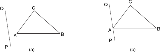
Although the faces of the objects we are dealing with can be polygons with any number of vertices, we will triangulate these polygons and use the resulting triangles instead. Suppose we are given a set of line segments PQ and a set of triangles ABC in terms of the eye and screen coordinates of all points P, Q, A, B and C. It will then be our task to draw each line segment PQ as far as none of the triangles ABC obscures them. A line segment (or line, for short) may be completely visible, completely invisible or partly visible. For example, in Figure 6.1, line 1 is completely visible because it lies in front of the triangle on the left and is unrelated to the other two triangles. In contrast, line 2 lies behind the triangle in the middle and is therefore completely invisible. Finally, lines 3 and 4 are not completely visible, but some parts of them are.
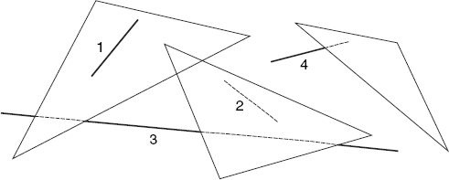
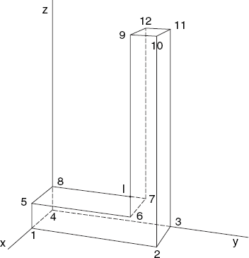
There is another important case: since the edges of the triangles are also line segments, it will frequently occur that a line segment is an edge of the triangle under consideration. Such line segments are to be considered visible, as far as that triangle is concerned. For example, consider the letter L in Figure 6.2. Here the only line segment that is partly visible and partly invisible is the line 7–8, which intersects the face 1-2-10-9-6-5, or rather one of the triangles (6-10-9, for example) of which this face consists. In the image, the line 7–8 intersects the edge 6–9 of that triangle in point I, which divides this line into the visible part 8-I and the invisible one I−7.
On the basis of the given faces of the object, we build a set of triangles and a set of line segments. Then for each line segment PQ, we call a method lineSegment, which has the task to draw any parts of PQ that are visible. This method is recursive and can be represented in the flowchart in Figure 6.3, where the numbered tests performed in different steps will be individually discussed in this section and the boxes with double edges denote recursive calls.
This flowchart is equivalent to the following pseudocode, in which I and J are points (between P and Q) of line segment PQ. On the screen we view I and J as intersecting points of PQ with edges of triangle ABC:
void lineSegment(line PQ, setsof triangles) { In sets, try to find a triangle ABC that obscures PQ (or part of it)
If no such triangle found,
      Draw PQ
  Else
  { If triangle ABC leaves part PI of PQ visible
     lineSegment(PI, the remaining triangles of s);    // Recursive call
  If triangle ABC leaves JQ of PQ visible
     lineSegment(JQ, the remaining triangles of s);    // Recursive call
  }
}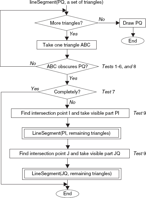
According to both the flowchart and this pseudocode, the loop that searches the set of triangles terminates as soon as a triangle ABC is found that obscures PQ. If ABC obscures PQ completely, no other action is required. If ABC obscures PQ partly, the parts that are possibly visible are dealt with recursively, using the remaining triangles. Note that in these cases the remaining triangles of the current loop are not applied to the whole line segment PQ anymore. The line PQ is drawn only if none of the triangles obscures it, that is, after the loop is completed.
To make the above algorithm as fast as we can, we should be careful with the order in which we perform several tests when we are looking for a triangle that obscures PQ. Tests that take little computing time and are likely to succeed are good candidates for being performed as soon as possible. Sometimes these aspects are contradictory. For example, in the sequence of tests that we will be discussing, the second is not very likely to succeed but it nevertheless deserves its position in this sequence because it is very inexpensive. The inner part of the loop that searches the set of triangles is discussed in greater detail below. Since we have to be careful with small numerical errors due to the finite precision of floating-point computations, we sometimes use small positive real numbers ɛ = eps as tolerances, as these examples show:
Mathematical expression | Implementation in program |
|---|---|
x ≤ a |
|
x < b |
|
y ≥ c |
|
y > d |
|
In the second column, it does not make any significant difference if we replace < with <=, and > with >=. We should take some care in choosing the value of eps, since this should preferably be related to the magnitude of the numbers we are comparing. You can find details of such tolerance values ɛ in the program file HLines.java, but they are omitted in the discussion below for the sake of clarity.
6.2.1 Test 1 (2D; Figure 6.4)
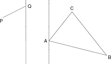
If neither P nor Q lies to the right of the leftmost one of the three vertices A, B and C (of triangle t) the triangle does not obscure PQ. This type of test is known as a minimax test: we compare the maximum of all x-coordinates of PQ with the minimum of all those of triangle t. Loosely speaking, we have now covered the case that PQ lies completely to the left of triangle t. In the same way, we deal with PQ lying completely to the right of t. Similar tests are performed for the minimum and maximum y-coordinates.
6.2.2 Test 2 (3D; Figure 6.5)
If PQ (in 3D space) is identical with one of the edges of triangle t, this triangle does not obscure PQ. This test is done very efficiently by using the vertex numbers of P, Q, A, B and C. As we will see in a moment, in recursive calls, P or Q may be a computed point, which has no vertex number. It is therefore not always possible to perform this test.

6.2.3 Test 3 (3D; Figure 6.6)
If neither P nor Q is further away than the nearest of the three vertices A, B and C of triangle t, this triangle does not obscure PQ. This is a minimax test, like Test 1, but this time applied to the z-coordinates. Since the positive z-axis points to the left in Figure 6.6, the greater the z-coordinate of a point, the nearer this point is. Therefore, triangle ABC does not obscure PQ if the minimum of zP and zQ is greater than or equal to the maximum of zA, zB and zC.
6.2.4 Test 4 (2D; Figure 6.7)
If, on the screen, the points P and Q lie on one side of the line AB while the third triangle vertex C lies on the other, triangle ABC does not obscure PQ.
The lines BC and CA are dealt with similarly. This test is likely to succeed, but we perform it only after the previous three tests because it is rather expensive. Since the vertices A, B and C are counter-clockwise, the points P and C are on different sides of AB if and only if the point sequence ABP is clockwise. As we have seen in Section 2.5, this implies that we can use the static method area2 of class Tools2D. With Point2D objects AScr, BScr, CScr for the points A, B and C, the left-hand side in the comparison
Tools2D.area2(AScr, BScr, PScr) <= 0
is equal to twice the area of triangle ABP, preceded by a minus sign if (and only if) the sequence ABP is clockwise. This value is negative if P and C lie on different sides of AB, and it is zero if A, B and P lie on a straight line. If this comparison succeeds and the same applies to
Tools2D.area2(AScr, BScr, QScr) <= 0
then the whole line PQ and point C lie on different sides of the line AB, so that triangle ABC does not obscure line segment PQ. After this test for the triangle edge AB, we use similar tests for edges BC and CA.
Note that P and Q can both lie outside triangle ABC, while PQ intersects this triangle. This explains the above test, which at first may look quite complicated. Unfortunately, the current test does not cover all cases in which PQ lies outside triangle ABC, as you can see in Figure 6.8.
6.2.5 Test 5 (2D; Figure 6.8)
Triangle ABC does not obscure PQ if the points A, B and C lie on the same side of the infinite line through P and Q. We determine if this is the case using a test that is similar to the previous one:
| (PQA ≤ 0 and PQB ≤ 0 and PQC ≤ 0) or |
| (PQA ≥ 0 and PQB ≥ 0 and PQC ≥ 0) |
where PQA, obtained as
double PQA = Tools2D.area2(PScr, QScr, AScr);
denotes twice the area of triangle PQA, preceded by a minus sign if the point sequence P, Q, A is clockwise. The variables PQB and PQC have similar meanings.
6.2.6 Test 6 (3D; Figure 6.9)
If neither P nor Q lies behind the plane through A, B and C, triangle ABC does not obscure PQ. This test deals with those line segments PQ for which Test 3 failed because the further one of the points P and Q does not lie nearer than the nearest of A, B, C, while P and Q nevertheless lie on the same side of the (infinite) plane ABC as the viewpoint E. Figure 6.9 illustrates this situation.
We now benefit from the fact that we have stored the normal vector n = (a, b, c) of plane ABC and the distance h between E and this plane. The equation of this plane is
ax + by + cz = h
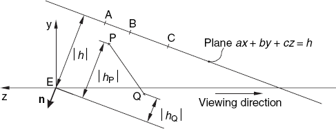
We compute
| hP = n · EP |
| hQ = n · EQ |
to perform the following test, illustrated by Figure 6.9:
| |hP| ≤ |h| and |hQ| ≤ |h| |
Since n, when starting at E, points away from the plane, the values of hP, hQ, like that of h, are negative, so that this test is equivalent to the following:
| hP ≥ h and hQ ≥ h |
6.2.7 Test 7 (2D; Figure 6.10)
If (on the screen) neither P nor Q lies outside the triangle ABC, and the previous tests were indecisive, PQ lies behind this triangle and is therefore completely invisible. The Tools2D method insideTriangle, discussed in Section 2.8, makes this test easy to program:
boolean pInside = Tools2D.insideTriangle(aScr, bScr, cScr, pScr);
boolean qInside = Tools2D.insideTriangle(aScr, bScr, cScr, qScr);
if (pInside && qInside) return;

The partial results of this test, stored in the boolean variables pInside and qInside, will be useful in Tests 8 and 9 in the case that this test fails.
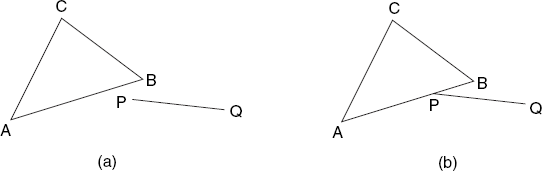
6.2.8 Test 8 (3D; Figure 6.11)
If P is nearer than the plane of triangle ABC and, on the screen, P lies inside triangle ABC, this triangle does not obscure PQ. The same is true for Q.
This test relies on the fact that no line segment PQ intersects any triangle. This test is easy to perform since the variables hP and hQ, computed in Test 6, and pInside and qInside, computed in Test 7, are now available. Using also the abbreviations pNear for hP > h and qNear for hQ > h, we conclude that triangle ABC does not obscure PQ if the following is true:
pNear && pInside || qNear && qInside
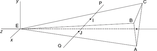
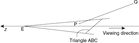
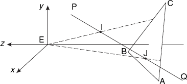
6.2.9 Test 9 (3D; Figure 6.12)
Although it might seem that, after Test 8, all cases with PQ not being obscured have been dealt with, this is not the case, as Figure 6.12 illustrates. In this example, Q lies behind the plane ABC, and, on the screen, PQ intersects ABC in the points I and J, but PQ is nevertheless completely visible (as far as triangle ABC is concerned). This is because both points of intersection, I and J, lie in front of (that is, nearer than) triangle ABC. We take three steps to deal with this situation:
We compute (the 2D projections of) I and J on the screen.
We compute the z-values of I and J by linear interpolation of 1/z (see Section 7.4 and Appendix A).
To determine if I and J lie in front of the plane ABC, we compute how far I and J lie away in the direction towards this plane.
We will now discuss these three steps in more detail, starting with step 1, which we deal with as a 2D problem, writing, for example, P for what is actually the projection P' of P on the screen.
Since we do not know in advance which of the three triangle edges AB, BC and CA may intersect PQ, we try all three by rotating the points A, B and C. Here we deal only with AB. Suppose that, on the screen, the infinite line PQ intersects the infinite line AB in point I, where
Then point I belongs to the line segments PQ and AB if and only if
| 0 ≤ λ ≤ 1 and 0 ≤ μ ≤ 1 |
While rotating A, B and C, we may find two points of intersection, with λ and μ satisfying these restrictions. We then denote the values λ of these points by λmin and λmax, and the corresponding points with I and J, so that we have
| 0 ≤ λmin < λmax ≤ 1 |
| PI = λminPQ |
| PJ = λmaxPQ |
As for the actual computation of λ and μ, let us use the vectors u = PQ and v = AB. It then follows from Equations (6.1) and (6.2) that we can express point I as the left- and right-hand sides of the following equation:
| P + λu = A + μv |
Writing w = PA (= A — P), we can replace this with
| λu — μv = w |
As usual, we write u = (u1, u2) and so on, which expands this vector equation to the following set of simultaneous linear equations:
| u1λ — v1μ = w1 |
| u2λ — v2μ = w2 |
Solving this system of equations, we obtain
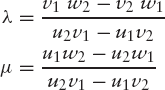
It goes without saying that this applies only if the denominators in these expressions are non-zero; otherwise PQ and AB are parallel, so that there are no points of intersection.
Having found the points I and J on the screen, we turn to step 2, to compute their z-coordinates. We do this by linear interpolation of 1/z on the segment PQ. Using the values λmin and λmax, which we have just found, and referring to Equation (6.1), we can write
Refer to the discussion in Section 7.4 and Appendix A about the reason why we should use 1/z instead of simply z in this type of linear interpolation.
Finally, we proceed to step 3, to determine whether or not the points I and J lie in front of the plane through the points A, B and C. Recall that the equation of this plane is
| ax + by + cz = h |
where h is negative, and that its normal vector (with length 1) is
| n = (a, b, c) |
We compute the value hI, which is similar to hP, discussed in Test 6 and illustrated by Figure 6.9, as
hI = EI · n = axI + byI + czI
After computing hJ similarly, we can now test if I and J lie in front of the plane ABC (so that triangle ABC does not obscure PQ) in the following way:
hI > h and hJ > h
In the above discussion, we considered two distinct points I and J in which, on the screen, PQ intersects edges of triangle ABC. As we have seen, PI and JQ were visible, as far as triangle ABC is concerned, but IJ may be obscured by triangle ABC. Actually, there may be only one point, I or J, to deal with. If, again on the screen, P lies outside triangle ABC and Q inside it, there is only point I to consider. In this case triangle ABC may obscure part IQ of line segment PQ. If it does, the remaining triangles are only to be applied to PI. Similarly, if, on the screen, P lies inside and Q outside triangle ABC, this triangle may obscure part PJ of PQ, and, if so, the remaining triangles are only to be applied to JQ.
If all the above tests fail, the most interesting (and time consuming) case applies: PQ is neither completely visible nor completely hidden. Fortunately, we have just computed the points of intersection I and J, and we know that triangle ABC obscures the segment IJ, while the other two segments, PI and QJ are visible, as far as triangle ABC is concerned. We therefore apply the method lineSegment recursively to the latter two segments. Actually, the recursive call for PI applies only to the case that, on the screen, P lies outside triangle ABC and λmin (see Test 9) is greater than zero. Analogously, the recursive call for QJ applies only if Q lies outside that triangle and λmax is less than 1.
In the paint method of the class CvHLines, we may be inclined to write the call to the method lineSegment in a very simple form, such as
lineSegment(g, iP, iQ);
where g is the graphics context and iP and iQ are the vertex numbers of the vertices P and Q. However, in the recursive calls just discussed, we have two new points I and J, for which there are no vertex numbers, so that this does not work. On the other hand, omitting the vertex numbers altogether would deprive us of Test 2 in its current efficient form, in which we determine if PQ is one of the edges of triangle ABC. We therefore decide to supply P and Q both as Point3D objects (containing the eye coordinates of P and Q) and as vertex numbers if this is possible; if it is not, we use −1 instead of a vertex number. When we recursively call lineSegment, the screen coordinates of P and Q are available. If we did not supply these as arguments, it would be necessary to compute them inside lineSegment once again. To avoid such superfluous actions, we also supply the screen coordinates of P and Q as arguments as Point2D objects. Finally, it would be a waste of time if the recursive calls would again be applied to all triangles. After all, we know that PI and PJ are not obscured by the triangles that we have already dealt with. We therefore also use the parameter iStart, indicating the start position in the array of triangles that is to be used. This explains that the method lineSegment has as many as eight parameters, as its heading shows:
void lineSegment(Graphics g, Point3D p, Point3D q,
   Point2D PScr, Point2D QScr, int iP, int iQ, int iStart)
The complete method lineSegment can be found in class CvHLines, listed in Appendix D.
From now on, we will no longer restrict ourselves to cubes, as we did in the previous chapter, but rather accept input files that define objects bounded by polygons (which may contain holes, as we will see in Section 6.4). These input files consist of two parts: a list of vertices, each in the form of a positive vertex number followed by three real numbers, the world coordinates of that vertex. The second part consists of an input line of the form
Faces:
followed by sequences of vertex numbers, each sequence followed by a period (.). Each such sequence denotes a polygon of the object. For each polygon, when viewed from outside the object, the vertex sequence must be counter-clockwise. This orientation must also apply to the first three vertices of each sequence; in other words, the second number of each sequence must denote a convex vertex. For example, the following input file, say, letterL.dat, describes the solid letter L of Figure 6.2:
1   20   0   0
 2   20  50   0
 3    0  50   0
 4    0   0   0
 5   20   0  10
 6   20  40  10
 7    0  40  10
 8    0   0  10
 9   20  40  80
10   20  50  80
11    0  50  80
12    0  40  80
Faces:
1  2  10  9  6  5.
3  4  8  7  12  11.
2  3  11  10.
7  6  9  12.
4  1  5  8.
9  10  11  12.
5  6  7  8.
1  4  3  2.
The first line after Faces specifies the front face. We might have used a different vertex-number sequence for this face, such as
10 9 6 5 1 2.
However, the following sequences would be incorrect:
2  1  5  6  9  10.   (invalid: clockwise)
9  6  5  1  2  10.   (invalid: 6 is not a convex vertex)
Although the sequence
3 4 8 7 12 11.
seems to be clockwise, it is really counter-clockwise when the face in question is viewed from outside the object, that is, from the back. As we will see in Section 7.1, we use this phenomenon in our programs to detect back faces.
In the first part of the input file, it is not required that the vertex numbers are consecutive and in ascending order. For example, the following input file (defining a pyramid similar to those in Egypt) is also acceptable. It also shows that the vertex coordinates need not be integers:
10   −1.5 −1.5  0
30    1.5 −1.5  0
20    1.5  1.5  0
12   −1.5  1.5  0
5     0    0    3
Faces:
30 20 5.
20 12 5.
12 10 5.
10 30 5.
30 10 12 20.
We will use the extension .dat for these input files.
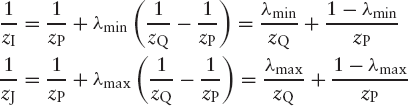
The above way of specifying the boundary faces of objects does not work for polygons that contain holes. For example, consider the solid letter A of Figure 6.13, the front face of which is not a proper polygon because there is a triangular hole in it. The same applies to the (identical) face on the back. Each vertex i of the front face is connected with vertex i + 10 of the back face (1 ≤ i ≤ 10).
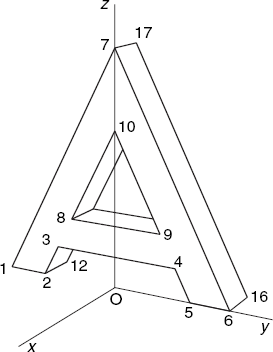
We can turn the front face into a polygon by introducing a very narrow gap, say, between the vertices 7 and 10, as shown in Figure 6.14. After doing this, we could try to specify this new polygon as
1 2 3 4 5 6 7 10 9 8 10 7.
Note that this requires the gap (7, 10) to have width zero, so that there is only one vertex (7) at the top. On the other hand, only a real gap makes it clear that the vertex numbers (10, 9, 8) occur in that order in the above input line: just follow the vertices in Figure 6.14, starting at vertex 1.
If we really specified the front face in the above way, the line (7, 10) would be regarded as a polygon edge and therefore appear in our result. This is clearly undesirable. To prevent this from happening, we adopt the convention of writing a minus sign in front of the second vertex of a pair, indicating that this pair denotes a line segment that is not to be drawn. We do this with the ordered pairs (7, 10) and (10, 7) in the above input line, writing (7, −10) and (10, −7), so that we use the following input line instead of the above one:
1 2 3 4 5 6 7 −10 9 8 10 −7.
The solid letter A of Figure 6.13 is therefore obtained by using the following input file, in which the extra minus signs occur in the first two lines after the word Faces:
1    0 −30   0
2    0 −20   0
3    0 −16   8
4    0  16   8
5    0  20   0
6    0  30   0
7    0   0  60
8    0 −12  16
9    0  12  16
10   0   0  40
11 −10 −30   0
12 −10 −20   0
13 −10 −16   8
14 −10  16   8
15 −10  20   0
16 −10  30   0
17 −10   0  60
18 −10 −12  16
19 −10  12  16
20 −10   0  40
Faces:
1 2 3 4 5 6 7 −10 9 8 10 −7.
11 17 −20 18 19 20 −17 16 15 14 13 12.
2 12 13 3.
3 13 14 4.
15 5 4 14.
8 9 19 18.
8 18 20 10.
19 9 10 20.
6 16 17 7.
11 1 7 17.
11 12 2 1.
15 16 6 5.
(Note that this use of minus signs applies only to vertex numbers in the second part of an input file. In the first part, minus signs can only occur in coordinate values, where they have their usual meaning.)
Implementing this idea is very simple. For example, because of the minus sign that precedes vertex number 10 in
... 7 −10 ...
we do not store line segment (7, 10) in the data structure that will be discussed in Section 6.5. In other respects, we simply ignore these minus signs. Therefore the set of triangles resulting from the above complete set of input data (for the solid letter A) is the same as when there had been no minus signs in front of any vertex numbers.
Besides for holes, we can also use these minus signs for the approximation for curved surfaces, as discussed in Section E.5 of Appendix E.
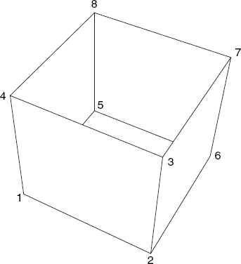
Although we usually draw polygons that are boundary faces of solid objects, we sometimes want to draw very thin (finite) planes, here also called faces. Examples are sheets of paper and a cube made of very thin material, of which the top face is removed, as shown in Figure 6.15.
Since such faces have two visible sides, we specify each face twice: counter-clockwise for the side we are currently viewing and clockwise for the side that is currently invisible but may become visible when we change the viewpoint. For example, the front face of the cube of Figure 6.15 is specified twice in the input file:
1 2 3 4.
4 3 2 1.
Although the user supplies polygons in input files as object faces, we deal primarily with line segments, referred to as PQ in the previous section. Besides the polygons and the triangles resulting from them, we also store the edges of the polygons as line segments. It is also desirable to be able to draw line segments that are not edges of polygons.
Examples of such 'loose', individual line segments are the axes of a 3D coordinate system. Sometimes we want to define the edges of polygons as individual line segments, to prevent such polygons from obscuring other line segments, displaying objects as wire-frame models. An example of this is shown in Figure 6.16. Here we have a solid pyramid fitting into a cube. Obviously, the pyramid would not be visible if the cube was solid; we therefore prefer the latter to be displayed as a wire-frame model. To provide an input file for this pyramid, we begin by assigning vertex numbers, as shown in Figure 6.17.
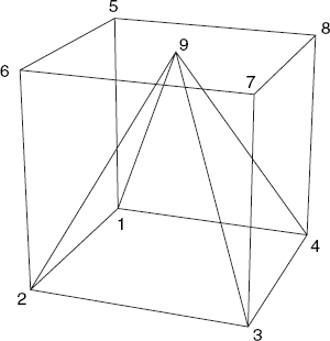
These vertex numbers occur in the following input file:
1  0 0 0
2  2 0 0
3  2 2 0
4  0 2 0
5  0 0 2
6  2 0 2
7  2 2 2
8  0 2 2
9  1 1 2
Faces:
1 4 3 2.
1 2 9.
2 3 9.
3 4 9.
4 1 9.
1 5.
2 6.
3 7.
4 8.
5 6.
6 7.
7 8.
8 5.
After the word Faces, we begin with the square bottom face and the four triangular faces of the pyramid. After this, four vertical and four horizontal cube edges follow, each specified by its two endpoints. It follows that the word Faces in our input files should not be taken too literally: this Faces section may include pairs of vertex numbers, which are not faces at all but line segments not necessarily belonging to faces.
Since line segments can occur not only as edges of faces but also individually, we have to design and implement a special data structure to store them in our program. This also provides us with the opportunity to store them only once. For example, the edge 3–9 of the pyramid of Figure 6.17 is part of the faces 2-3-9 and 3-4-9, but it would be inefficient to draw it twice. By using a special data structure for line segments, we can ensure that this edge is stored only once.
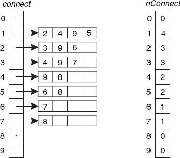
Our data structure for line segments will be based on an array of arrays, as shown on the left in Figure 6.18.
An array element connect[i] referring to an array containing the integer j implies that there is a line segment (i, j) to be drawn. By requiring that i is less than j, we ensure that each line segment is stored only once. For example, connect[1] refers to the array containing the integers 2, 4, 9 and 5. This indicates that the following line segments start at vertex 1 (each ending at a vertex that has a number higher than 1): 1–2, 1–4, 1–9 and 1–5, which is in accordance with Figure 6.17. The next element, connect[2] refers to three vertex numbers, 3, 9 and 6. Although, besides 2–3, 2–9 and 2–6, there is also a line segment 2-1 (see Figure 6.17), this is not included here because 2 is greater than 1 and this segment has already been stored as line segment 1–2. You may wonder why in Figure 6.18 there are only boxes that give room for at most four vertex numbers. Actually, the sizes of these boxes will always be a multiple of some chunk size, here arbitrarily chosen as 4. In other words, if there are five line segments (i, j) with the same i and all with i less than j, the box size would be increased from 4 to 8 and so on. Since increasing the box size requires memory reallocation and copying, we should not choose the chunk size too small. On the other hand, the larger the chunk size, the more memory will be wasted, since they will normally not be completely filled. To indicate how many vertex numbers are actually stored in each box, we use another array, nConnect, as shown in Figure 6.18 on the right. For example, nConnect[1] = 4 because connect[1] refers to four vertex numbers.
As long as 3D objects do not have too many vertices and the vertex coordinates are easily available, it is not difficult to create 3D specifications as input files by entering all data manually, using a text editor. This is the case, for example, with the solid letter A, discussed in Section 6.4. If there are many vertices, which is normally the case if we approximate curved surfaces, we had better generate 3D data files by special programs. This section explains how to automatically generate 3D specifications through an example. The generated specification files are accepted by the programs Painter.java, ZBuf.java (for hidden-face elimination, described in Chapter 7) and HLines.java (for hidden-line elimination, described in the next two sections). Most illustrations in this chapter have been obtained by using HLines.java for this purpose.
Many 3D objects are bounded by curved surfaces. We can approximate these by a set of polygons. An example is a hollow cylinder as shown in Figure 6.19 on the right. Both representations of hollow cylinders (or rather, hollow prisms) of Figure 6.19 were obtained by running the program Cylinder.java, which we will be discussing, followed by the execution of program HLines.java. HP-GL files exported by the latter program were combined by CorelDraw, after which the result was imported into this book. Although the object shown on the left in Figure 6.19 is a (hollow) prism, not a cylinder, we will consistently use the term cylinder in this discussion.
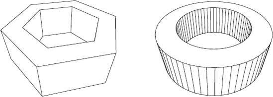
The user will be able to enter the diameters of both the (outer) cylinder and the (inner) cylindrical hole. If the latter, smaller diameter is zero, our program will produce a solid cylinder instead of a hollow one. For simplicity, we will ignore this special case, with only half the number of vertices, in our discussion below, but simply implement it in the program.
For some sufficiently large integer n (not less than 3), we choose n equidistant points on the outer circle (with radius R) of the top face, and we choose n similar points on the bottom face. Then we approximate the outer cylinder by a prism whose vertices are these 2n points. The inner circle (of the cylindrical hole) has radius r (< R). The hollow cylinder has height h. Let us use the z-axis of our coordinate system as the cylinder axis. The cylindrical hole is approximated by rectangles in the same way as the outer cylinder. The bottom face lies in the plane z = 0 and the top face in the plane z = h. A vertex of the bottom face lies on the positive x-axis. Let us set h = 1. Then for given values n, R and r, the object to be drawn and its position are then completely determined. We shall first deal with the case n = 6 and generalize this later for arbitrary n. We number the vertices as shown in Figure 6.20.
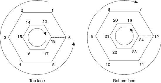
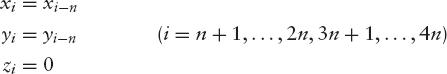
For each vertex i of the top face there is a vertical edge that connects it with vertex i + 6. We can specify the top face by the following sequence:
1 2 3 4 5 6 −18 17 16 15 14 13 18 −6.
Here the pairs (6, – 18) and (18, – 6) denote an artificial edge, as discussed in Section 6.4. The bottom face on the right is viewed here from the positive z-axis, but in reality only the other side is visible. The orientation of this bottom face is therefore opposite to what we see in Figure 6.20 on the right, so that we can specify this face as
12 11 10 9 8 7 −19 20 21 22 23 24 19 −7.
Since n = 6, we have 12 = 2n, 18 = 3n and 24 = 4n, so the above sequences are special cases of
| 1 2 . . . n − 3n 3n − 1 3n − 2 . . . 2n + 1 3n − n. |
and
| 2n 2n − 1 . . . n + 1 − (3n + 1) 3n + 2 3n + 3 . . . 4n |
| 3n + 1 − (n + 1). |
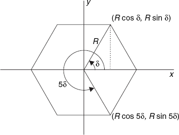
Let us define
Since, in Figure 6.20, on the left, vertex 6 lies on the positive x-axis and according to geometry in Figure 6.21 (outer circle), the Cartesian coordinates of the vertices on the top face are as follows:
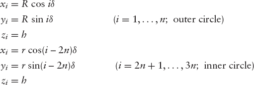
For the bottom face we have
A program based on the above analysis can be written in any programming language. Using Java for this purpose, we can choose between an old-fashioned, text-line oriented solution and a graphical user interface with, for example, a dialog box with text fields and a button as shown in Figure 6.22.
This dialog box contains a title bar, and seven so-called components: three labels (that is, static text in the gray area), three text fields in which the user can enter data, and an OK button. Programming the layout of a dialog box in Java can be done in several ways, none of which is particularly simple. Here we do this by using three panels:
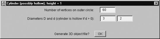
Panel p1 at the top, or North, for both the label Number of vertices on outer circle and a text field in which this number is to be entered.
Panel p2 in the middle, or Center, for the label Diameters D and d (cylinder is hollow if d > 0) and two text fields for these diameters.
Panel p3 at the bottom, or South, for the label Generate 3D object file? and an OK button.
Since there are only a few components in each panel, we can use the default FlowLayout layout manager for the placements of these components in the panels. By contrast, the panels are placed above one another by using BorderLayout, as the above words North, Center and South, used in the program as character strings, indicate. As in many other graphics programs in this book, we use two classes in this program, but this time there is a dialog class instead of a canvas class. Another difference is that we do not display the frame, but restrict the graphical output to the dialog box. (We cannot omit the frame class altogether because the Dialog constructor requires a 'parent frame' as an argument.) Recall that we previously used calls to setSize, setLocation and show in the constructor of the frame class. We simply omit these calls to prevent the frame from appearing on the screen. Obviously, we must not omit such calls in the constructor of our dialog class, called DlgCylinder in the program. As for the generation of the hollow cylinder itself, as discussed above, this can be found in the method genCylinder, which follows this constructor:
// Cylinder.java: Generating an input file for a
//                (possibly hollow) cylinder.
import java.awt.*;
import java.awt.event.*;
import java.io.*;

public class Cylinder extends Frame
{  public static void main(String[] args){new Cylinder();}
   Cylinder(){new DlgCylinder(this);}
}

class DlgCylinder extends Dialog
{  TextField tfN = new TextField (5);
   TextField tfOuterDiam = new TextField (5);
   TextField tfInnerDiam = new TextField (5);
   Button button = new Button("  OK  ");
   FileWriter fw;

   DlgCylinder(Frame fr)
   {  super(fr, "Cylinder (possibly hollow); height = 1", true);
      addWindowListener(new WindowAdapter()
      {  public void windowClosing(WindowEvent e)
         {  dispose();
            System.exit(0);
         }
      });
      Panel p1 = new Panel(), p2 = new Panel(), p3 = new Panel();
      p1.add(new Label("Number of vertices on outer circle: "));
      p1.add(tfN);
      p2.add(new Label(
         "Diameters D and d (cylinder is hollow if d > 0): "));
      p2.add(tfOuterDiam); p2.add(tfInnerDiam);
      p3.add(new Label("Generate 3D object file?"));
      p3.add(button);
      setLayout(new BorderLayout());
      add("North", p1);
      add("Center", p2);
      add("South", p3);

      button.addActionListener(new ActionListener()
      {  public void actionPerformed(ActionEvent ae)
         {  int n=0;
            float dOuter=0, dInner=0;
            try
            {  n = Integer.valueOf(tfN.getText()).intValue();
               dOuter =
                  Float.valueOf(tfOuterDiam.getText()).floatValue();
               dInner =
                  Float.valueOf(tfInnerDiam.getText()).floatValue();
               if (dInner > 0) dInner = 0;
if (n < 3 || dOuter <= dInner)
Toolkit.getDefaultToolkit().beep();
else
{ try
{ genCylinder(n, dOuter/2, dInner/2);
}
catch (IOException ioe){}
dispose();
System.exit(0);
}
}
catch (NumberFormatException nfe)
{ Toolkit.getDefaultToolkit().beep();
}
}
});
Dimension dim = getToolkit().getScreenSize();
setSize(3 * dim.width/4, dim.height/4);
setLocation(dim.width/8, dim.height/8);
show();
}
void genCylinder(int n, float rOuter, float rInner)
throws IOException
{ int n2 = 2 * n, n3 = 3 * n, n4 = 4 * n;
fw = new FileWriter("Cylinder.dat");
double delta = 2 * Math.PI / n;
for (int i=1; i<=n; i++)
{ double alpha = i * delta,
cosa = Math.cos(alpha), sina = Math.sin(alpha);
for (int inner=0; inner<2; inner++)
{ double r = (inner == 0 ? rOuter : rInner);
if (r > 0)
for (int bottom=0; bottom<2; bottom++)
{ int k = (2 * inner + bottom) * n + i;
// Vertex numbers for i = 1:
// Top: 1 (outer) 2n+1 (inner)
// Bottom: n+1 (outer) 3n+1 (inner)
wi(k); // w = write, i = int, r = real
wr(r * cosa); wr(r * sina); // x and y
wi(1 - bottom); // bottom: z = 0; top: z = 1
fw.write("
");
}}
}
fw.write("Faces:
");
// Top boundary face:
for (int i=1; i<=n; i++) wi(i);
if (rInner > 0)
{ wi(-n3); // Invisible edge, see Section 7.5
for (int i=n3-1; i>=n2+1; i--) wi(i);
wi(n3); wi(-n); // Invisible edge again.
}
fw.write(".
");
// Bottom boundary face:
for (int i=n2; i>=n+1; i--) wi(i);
if (rInner > 0)
{ wi(-(n3+1));
for (int i=n3+2; i<=n4; i++) wi(i);
wi(n3+1); wi(-(n+1));
}
fw.write(".
");
// Vertical, rectangular faces:
for (int i=1; i<=n; i++)
{ int j = i % n + 1;
// Outer rectangle:
wi(j); wi(i); wi(i + n); wi(j + n); fw.write(".
");
if (rInner > 0)
{ // Inner rectangle:
wi(i + n2); wi(j + n2); wi(j + n3); wi(i + n3);
fw.write(".
");
}
}
fw.close();
}
void wi(int x)
throws IOException
{ fw.write(" " + String.valueOf(x));
}
void wr(double x)
throws IOException
{ if (Math.abs(x) < 1e-9) x = 0;
fw.write(" " + String.valueOf((float)x));// float instead of double to reduce the file size } }
The number 60 entered in the top text field of Figure 6.22 refers to the hollow cylinder shown in Figure 6.19 on the right. The hollow prism shown on the left in this figure is obtained by replacing 60 with 6. In that case the following file is generated:
1 0.75 1.299038 1
 7 0.75 1.299038 0
 13 0.5 0.8660254 1
 19 0.5 0.8660254 0
 2 −0.75 1.299038 1
 8 −0.75 1.299038 0
 14 −0.5 0.8660254 1
 20 −0.5 0.8660254 0
 3 −1.5 0.0 1
 9 −1.5 0.0 0
 15 −1.0 0.0 1
 21 −1.0 0.0 0
 4 −0.75 −1.299038 1
 10 −0.75 −1.299038 0
 16 −0.5 −0.8660254 1
 22 −0.5 −0.8660254 0
 5 0.75 −1.299038 1
 11 0.75 −1.299038 0
 17 0.5 −0.8660254 1
 23 0.5 −0.8660254 0
 6 1.5 0.0 1
 12 1.5 0.0 0
 18 1.0 0.0 1
 24 1.0 0.0 0
Faces:
 1 2 3 4 5 6 −18 17 16 15 14 13 18 −6.
 12 11 10 9 8 7 −19 20 21 22 23 24 19 −7.
 2 1 7 8.
 13 14 20 19.
 3 2 8 9.
 14 15 21 20.
 4 3 9 10.
 15 16 22 21.
 5 4 10 11.
16 17 23 22.
 6 5 11 12.
 17 18 24 23.
 1 6 12 7.
 18 13 19 24.
Recall that we have already discussed the first two lines that follow the word Faces. More interesting examples on generating input files for different 3D objects can be found in Appendix E.
HIDDEN-LINE ELIMINATION WITH HP-GL OUTPUT
Besides graphics output on the screen, it is sometimes desired to produce output files containing the same results. An easy way to realize this for line drawings is by using the file format known as HP-GL, which stands for Hewlett-Packard Graphics Language. We will use only a very limited number of HP-GL commands:
IN: Initialize
SP: Set pen
PU: Pen up
PD: Pen down
PA: Plot absolute
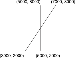
We think of drawing by moving a pen, which can be either on or above a sheet of paper. These two cases are distinguished by the commands PD and PU. The PA command is followed by a coordinate pair x, y, each as a four-digit integer in the range 0000–9999. This coordinate pair indicates a point that the pen will move to. The origin (0000, 0000) lies in the bottom-left corner. For example, the following HP-GL file draws a capital letter X in italic, shown in Figure 6.23:
IN;SP1;
PU;PA5000,2000;PD;PA5000,8000;
PU;PA3000,2000;PD;PA7000,8000;
This file format is easy to understand and it is accepted by many well-known packages, such as Microsoft Word and CorelDraw. The latter enables us to enhance the drawing after importing the HP-GL file, as was done to add text, resulting in Figure 6.23.
We will see how to implement this in the next section.
The program HLines.java is listed in Appendix D. First, HLines.java can generate HP-GL files (Figure 6.24 illustrates a menu item for exporting HP-GL files); second, it can display individual lines, and third, printing and photocopying the resulting images can be done in black and white without loss of quality. On the contrary, these line drawings, obtained via HP-GL files and produced by a printer, look better than those on the screen.
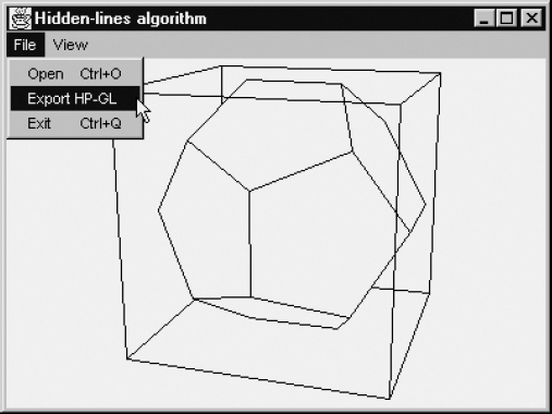
This example also shows the use of individual line segments, as discussed in Section 6.5. The solid inside the wire-frame cube is a dodecahedron, which is discussed in greater detail in Section E.1 of Appendix E.
The statement
cv.setHPGL(new HPGL(obj));
in the class MenuCommands (at the end of the file HLines.java) creates an object of class HPGL, and the variable hpgl of the class CvHLines is made to refer to it. The fact that hpgl is no longer equal to null will be interpreted as an indication that an HP-GL file is to be written. The class HPGL can be found at the end of Appendix D. The write method of this class is used in the drawLine method of the class CvHLines, that is, if the variable hpgl is unequal to null, as discussed above. After we have written an HP-GL file, we set hpgl equal to null again (at the end of the paint method) to avoid that every call to paint should automatically produce HP-GL output. If this is again desired, the user must use the Export HP-GL command of the File menu once again. The class CvHLines is defined in the file HLines.java (see Appendix D).
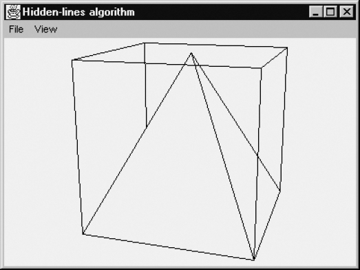
Figure 6.25 shows that our hidden-line algorithm can correctly render the three beams that we will use to demonstrate the Z-buffer algorithm for hidden-face elimination. As we will see in Section 7.3, the painter's algorithm fails in this case.
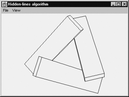
The program HLines.java has much in common with Wireframe.java, discussed at the end of Chapter 5. We will therefore benefit as much as possible from the code that we have already developed in Section 5.5. Unfortunately, since we now have an extra menu item, Export HPGL, in the File menu, we cannot use the existing frame class Fr3D directly, but we will use an extended version, that is, a subclass of it. The name of this subclass, Fr3DH, occurs in the main method of the following file:
// HLines.java: Perspective drawing with hidden-line elimination.
// When you compile this program, the .class or the .java files of the
// following classes should also be in your current directory:
//       CvHLines, Fr3D, Fr3DH, Polygon3D, Obj3D, Input, Canvas3D,
//       Point3D, Point2D, Triangle, Tria, Tools2D, HPGL.
import java.awt.*;
import java.awt.event.*;
import java.util.*;

public class HLines extends Frame
{  public static void main(String[] args)
   {  new Fr3DH(args.length > 0 ? args[0] : null, new CvHLines(),
         "Hidden-lines algorithm");
   }
}
Notice the title Hidden-lines algorithm, which is used here as the third argument of the Fr3DH constructor, and consequently appears in the title bar of the window shown in Figure 6.25. The implementation of the hidden-lines algorithm discussed in this chapter can be found in the class CvHLines, of which an object is created in the second argument of the above constructor call. In view of the extent of this class, it is not listed here but rather as the file CvHLines.java in Appendix D. In this section we will only discuss some other aspects of the program, especially some classes occurring in the above comment lines, as far as these have not been dealt with in Section 5.5.
The subclass Fr3DH, just mentioned, of Fr3D is defined in the following file:
// Fr3DH.java: Frame class for HLines.java.
// This class extends Fr3D to enable writing HP-GL output files.
import java.awt.*;
import java.awt.event.*;
import java.util.*;

class Fr3DH extends Fr3D
{  private MenuItem exportHPGL;
   CvHLines cv;
Fr3DH(String argFileName, CvHLines cv, String textTitle)
{ super(argFileName, cv, textTitle);
exportHPGL = new MenuItem("Export HP-GL");
mF.add(exportHPGL);
exportHPGL.addActionListener(this);
this.cv = cv;
}
public void actionPerformed(ActionEvent ae)
{ if (ae.getSource() instanceof MenuItem)
{ MenuItem mi = (MenuItem)ae.getSource();
if (mi == exportHPGL)
{ Obj3D obj = cv.getObj();
if (obj != null)
{ cv.setHPGL(new HPGL(obj));
cv.repaint();
}
else
Toolkit.getDefaultToolkit().beep();
}
else
super.actionPerformed(ae);
}
}
}At the start of the class, the variable exportHPGL is declared to implement the additional menu item that we need. The method actionPerformed overrides the method with the same name of the super class Fr3D. When any menu command is used, a test is executed to see if this command is Export HPGL. If this is not the case, the method actionPerformed of the super class is called to deal with other menu commands. If it is the case, the statement
cv.setHPGL(new HPGL(obj));
is executed, which makes a variable hpgl of the class CvHlines point to an HPGL object, generated here as an argument of setHPGL. By making this variable hpgl unequal to null, any call of the CvHLines method drawLine will perform the desired HP-GL output, as you can see in the following lines, copied from Appendix D.
private void drawLine(Graphics g, float x1, float y1,
float x2, float y2)
{  if (x1 != x2 || y1 != y2)
   {  g.drawLine(iX(x1), iY(y1), iX(x2), iY(y2));
      if (hpgl != null)
      {  hpgl.write("PU;PA" + hpx(x1) + "," + hpy(y1));
         hpgl.write("PD;PA" + hpx(x2) + "," + hpy(y2) + "
");
      }
   }
}
To clarify both the use of the HPGL constructor in the above call of setHPGL and this method drawLine, we will also have a look at the way the class HPGL is defined:
// HPGL.java: Class for export of HP-GL files.
import java.io.*;

class HPGL
{  FileWriter fw;
   HPGL(Obj3D obj)
   {  String plotFileName = "", fName = obj.getFName();
      for (int i=0; i<fName.length(); i++)
      {  char ch = fName.charAt(i);
         if (ch == stquote.stquote) break;
         plotFileName += ch;
      }
      plotFileName += ".plt";
      try
      {  fw = new FileWriter(plotFileName);
         fw.write("IN;SP1;
");
      }
      catch (IOException ioe){}
   }

   void write(String s)
   {  try {fw.write(s); fw.flush();}catch (IOException ioe){}
   }
}
Apart from the extra code to generate HP-GL output and the obvious greater complexity of the canvas class due to hidden-line elimination, the structure of program HLines.java is very similar to Wireframe.java discussed at the end of the previous chapter.
EXERCISES
6.1 Use a normal editor or text processor to create a data file, to be used with program HLines.java, for the object consisting of both a horizontal square and a vertical line through its center, as shown twice in Figure 6.26. On the left the viewpoint is above the square (as it is by default), while the situation on the right, with the viewpoint below the square, has been obtained by using the Viewpoint Down command of the View menu (or by pressing Ctrl+↓).

6.2 Hidden-line elimination works correctly for the problem in Exercise 6.1 because the vertical line passes through edges of the triangles produced by triangulation of the square. Change the horizontal square to a horizontal triangle and use HLines.java to display the object with the same vertical line through the triangle. The object may not be displayed properly like those in Figure 6.26. Explain why and find a simple solution.
6.3 The same as Exercise 6.1 for Figure 6.27, which shows two very thin square rings. Again, the object is shown twice to demonstrate that there are four potentially visible faces.
6.4 Write a program HLinesDashed.java similar to HLines.java but instead of omitting hidden lines, draw them as dashed lines. For example, when applied to the file letterL.dat of Section 6.3, it produces the result of Figure 6.28 (after changing the viewpoint). An easy way of doing this is by letting the method lineSegment in your class CvHLinesDashed first draw the whole line PQ as a dashed line, so these dashed lines, or parts of them, will later be overwritten by normally drawn lines if the line segments in question happen to be visible. Note that this should happen only for calls to lineSegment from the paint method, not for recursive calls. You can use a method dashedLine similar to the one of Exercise 1.5. This call to dashedLine can be followed by a fragment of the form
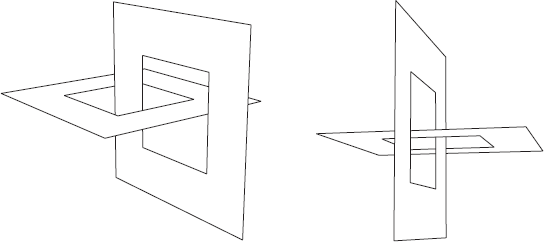
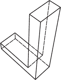
Figure 6.28. Hidden lines represented by dashed lines
if (hpgl != null)
{  hpgl.write("LT4 1;
");
   ...
   hpgl.write("LT;
");
}
where . . . denotes two lines similar to those for HP-GL output in the method drawLine. This will make dashed lines also appear in HP-GL output when the user uses the Export HP-GL command. The two HP-GL commands LT shown here will switch from normally drawn to dashed lines, and back to normal lines.
For each of Exercises 6.5–6.10, you are to write a program that generates a 3D object file in the format discussed in Sections 6.3–6.5. You may refer to Appendix E for more relevant examples. The files generated by your program can be read by not only the program HLines.java, but also the programs Painter.java and ZBuf.java described in Chapter 7.
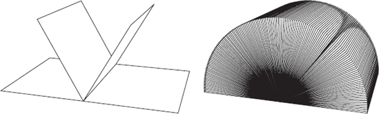
6.5 Write a program BookView.java that can generate a data file for an open book. Enable the user to supply the number of sheets, the page width and height, and the name of the output file as program arguments. For example, the files bookv4.dat and bookv150.dat for the books shown in Figure 6.29 were obtained by executing the following commands:
java BookView 4 15 20 bookv4.dat
java BookView 150 15 20 bookv150.dat
Apply the program HLines.java to it to generate HP-GL files. Import these files into a text processor or drawing program, as was done twice for Figure 6.29.
6.6 Write a program to generate a globe model of a sphere, as shown in Figure E.4 of Appendix E. Enable the user to supply n (see Section E.2) as a program argument.
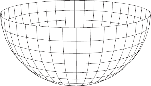
6.7 Write a program to generate a semi-sphere, as shown in Figure 6.30.
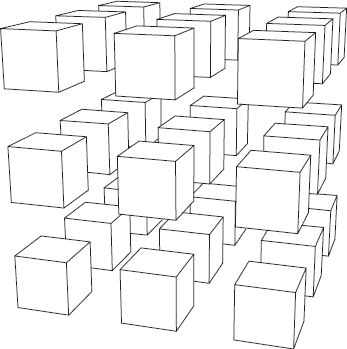
6.8 Generate a great many cubes that are placed beside, behind and above each other (see Figure 6.31).
6.9 Generate a data file for two tori (the plural of torus), as shown in Figure 6.32.

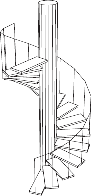
6.10 Write a program to generate a spiral staircase, as shown in Figure 6.33.