5.5 Parametric stereo decoder

The structure of the parametric stereo decoder is shown in Figure 5.3. The mono input signal s₁ is first processed by a hybrid QMF analysis filterbank. Subsequently, the hybrid QMF-domain signal s_1,m is processed by a decorrelator (D) to result in a second signal D(s_1,m). These two input signals are processed by a matrix R_b. Finally, two hybrid QMF synthesis filterbanks generate the two domain–domain output signals ₁ and ₂. These separate stages will be explained in more detail in the following sections.

5.5.1 Analysis filterbank

The applied filterbank is a hybrid complex-modulated quadrature mirror filter bank (QMF) which is an extension to the filterbank as used in spectral band replication (SBR) techniques [68, 172, 279]. The hybrid QMF analysis filterbank consists of a cascade of two filterbanks. The structure is shown in the left panel of Figure 5.4.

The first filterbank (QMF analysis) is compatible with the filterbank as used in SBR. The sub-band signals which are generated by this first filterbank are obtained by convolving the input signal with a set of analysis filter impulse responses G_m0(n) given by

with g₀(n) for n = 0,..., N₀ − 1 the prototype window of the filter, M₀ = 64 the number of output channels, m₀ the sub-band index (m₀ = 0,...,M − 1), and N₀ = 640 the filter length. The filtered outputs are subsequently down sampled by a factor M₀, to result in a set of down-sampled QMF outputs (or sub-band signals) s_1,m0 (the equations given here are purely analytical; in practice the computational efficiency of the filter bank can be increased using decomposition methods).

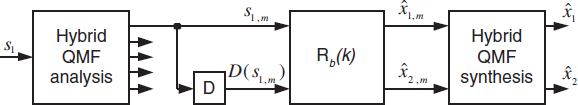
Figure 5.3 Structure of the QMF-based decoder. The signal is first fed through a hybrid QMF analysis filter bank. The filterbank output and a decorrelated version of each filterbank signal is subsequently fed into a matrixing stage R_b(k). Finally, two hybrid QMF synthesis banks generate the two output signals.

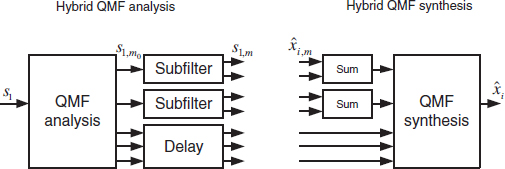
Figure 5.4 Structure of the hybrid QMF analysis (left panel) and synthesis (right panel) filter banks.

The magnitude responses of the first four frequency bands (m₀ = 0..3) of the QMF analysis bank are illustrated in Figure 5.5.

The down-sampled sub-band signals s₁,m₀ of the lowest QMF sub-bands are subsequently fed through a second complex-modulated filter bank (sub-filterbank) of order N₁ to further enhance the frequency resolution; the remaining sub-band signals are delayed by N₁/2 samples to compensate for the delay which is introduced by the sub-filterbank. The output of the hybrid (i.e., combined) filterbank is denoted by s_1,m, with m the index of the hybrid QMF bank. To allow easy identification of the two filterbanks and their outputs, the index m₀ of the first filterbank will be denoted ‘sub-band index’, and the index m₁ of the sub-filterbank is denoted ‘sub-sub-band index’. The sub-filterbank has a filter order of N₁ = 12, and an impulse response G_m1(k) given by

with g₁(k) the prototype window, k the sub-band sample index, and M₁ the number of sub-sub-bands. Table 5.3 gives the number of sub-sub-bands M₁(m₀) as a function of the QMF band m₀, for both the 34 and 20 analysis-band configurations. As an example the magnitude response of the 4-band sub-filterbank (M₁ = 4) is given in Figure 5.6.

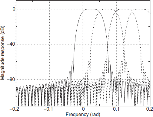
Figure 5.5 Magnitude responses of the first 4 of the 64 bands SBR complex-exponential modulated analysis filterbank. The magnitude for m₀ = 0 is highlighted.

Table 5.3 Specification of M₁ for the first 5 QMF sub-bands.

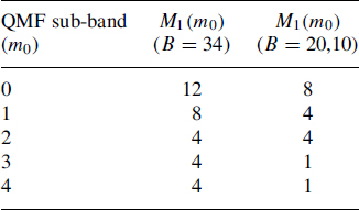
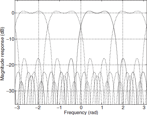
Figure 5.6 Magnitude response of the 4-band sub-filterbank (M₁ = 4). The response for m₁ = 0 is highlighted.

Obviously, due to the limited prototype length (N₁ = 12), the stop-band attenuation is only in the order of 20 dB.

As a result of this hybrid QMF filterbank structure, 91 (for B = 34) or 77 (B = 20 or 10) down-sampled filter outputs s_1,m are available for further processing.

5.5.2 Decorrelation

In order to generate two output signals with a variable (i.e., parameter–dependent) coherence, a second signal is generated which has a similar spectral-temporal envelope as the mono input signal, but is incoherent from a fine-structure waveform point of view. This incoherent (or orthogonal) signal, D(s_1,m) is generated by the decorrelator (D), and is obtained by convolving the mono input signal with an all-pass filter. The decorrelation is performed in the QMF domain as shown in Figure 5.3. A very cost-effective decorrelation all-pass filter is obtained by a simple (frequency-dependent) delay. The combination of a delay and a (fixed) mixing matrix to produce two signals with a certain spatial diffuseness is known as a Lauridsen decorrelator [179]. The structure of a Lauridsen decorrelator is shown in Figure 5.7. The input signal s is delayed (T), attenuated (G) and added (₁) or subtracted (₂) from the input. The decorrelation is produced by complementary combfilter peaks and troughs in the two output signals resulting from different signs in the combination of the direct and delayed signals.

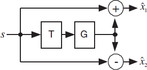
Figure 5.7 Structure of a Lauridsen decorrelator.

The attenuation (G) associated with the delayed signal determines the coherence of the two output signals. A low value for G will result in a high coherence, while a value for G of +1 will result in fully decorrelated signals. The coherence c_x1x2 is given by:

The delay T determines the spectral spacing of the comb filter. A longer delay results in a higher density of peaks and troughs. This can be observed from Figure 5.8. The top panel shows the two output spectra (represented by the solid and dashed lines, respectively) for a delay of T = 5 ms and a gain G = 1. For the lower panel, these parameters are 10 ms and 0.5, respectively. The longer delay clearly results in a more dense harmonic spectra, while the lower value of the gain results in a decrease in the depth of the spectral peaks and troughs.

This Lauridsen decorrelator works reasonably well provided that the delay is sufficiently long to result in multiple comb-filter peaks and troughs in each auditory filter. Due to the fact that the auditory filter bandwidth is larger at higher frequencies, the delay is preferably frequency dependent, being shorter at higher frequencies to prevent audible ‘doubles’ or ‘echos’. A frequency-dependent delay has the additional advantage that it does not result in harmonic comb-filter effects in the output. To further increase the density of the comb-filter peaks and troughs, the parametric stereo decoder features a combination of a frequency-dependent delay, an IIR allpass filter to mimic properties of late reverberation, and a ducking mechanism to remove undesirable reverberation tails if the input signal exhibits a sudden strong decrease in energy. More information on the decorrelation all-pass filter can be found in [79].

One important aspect of the signal combination (or matrixing) that is applied in the Lauridsen decorrelator is that the single gain for mixing the delayed signal into both output channels with equal gain, but reversed phase is that this is only one of an infinite number possible realizations to realize a specific correlation. More specifically, the amount of decorrelation signal can be made smaller by introducing individual mixing control for each of the two output channels individually, resulting in a higher output quality. This will be outlined in the next section.

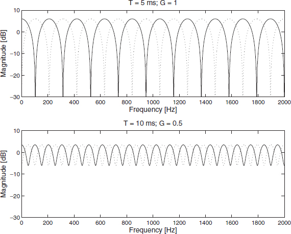
Figure 5.8 Spectra resulting from the Lauridsen decorrelator for T = 5 ms, G = 1 (top panel) and T = 10 ms, G = 0.5 (lower panel). The solid line represents output ₁, the dotted line corresponds to ₂.

5.5.3 Matrixing

The matrixing stage R_b of the QMF-based spatial synthesis process performs a mixing and phase-adjustment process. For each sub-sub-band signal pair s_1,m, D(s_1,m), an output signal pair _1,m, _2,m is generated by:

The mixing matrices R_b are determined by the following constraints:

1. The coherence of the two output signals must obey the transmitted ICC parameter.
2. The power ratio of the two output signals must obey the transmitted ICLD parameter.
3. The average energy of the two output signals must be equal to the energy of the mono input signal.
4. The average phase difference between the output signals must be equal to the transmitted ICPD value.
5. The average phase difference between s_1,m and x_1,m should be equal to the OCPD value.

Rotator ‘A’

The parametric stereo decoder features two methods to re-create signals with the correct spatial properties. The first method, labelled ‘A’, aims at reconstruction of ICLDs and ICCs, without incorporation of phase differences (ICPD and OCPD). Due to the absence of ICPD parameters, the ICC parameter has a range of −1 to +1, and hence the mixing matrix should be designed in such a way that it can cope with this large correlation range in a robust way.

Synthesis of the correct ICC parameter using rotator ‘A’ can be understood by making the following matrix decomposition of the mixing matrix R_b:

with H_b a real-valued matrix to set the correct ICC parameter, and Q_b a diagonal, realvalued matrix that ensures the correct ICLD parameters by real-valued scaling. A suitable representation of the matrix H is given by:

A visual interpretation of this matrix is shown in the left panel of Figure 5.9. The horizontal and vertical axes represent the two input signals s_1,m and D(s_1,m). Each output signal (_1,m and _2,m) is represented by a vector in the two-dimensional signal space. The two vectors have an angular difference of 2α and a mean (or common) rotation angle of β. The orthogonality property of the two input signals guarantees a fixed amount of energy that is represented by the length of the output vectors, independent of the two rotation angles α and β.

There exists a unique relation between the ICC parameter c₁₂ and the rotation angle α which is given by:

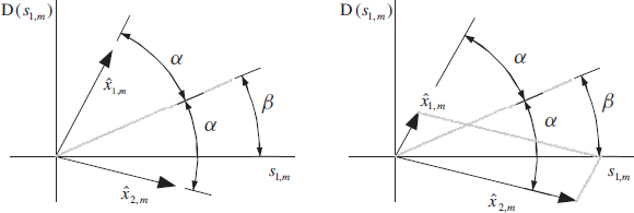
Figure 5.9 Visualization of rotator type ‘A’.

Thus, the ICC value is independent of the overall rotation angle β. In other words, there exists an infinite number of solutions to combine two independent signals to create two output signals with a specified ICC value. In Figure 5.9, this is represented by the free choice of the angle β. The solution for β for rotator ‘A’ was chosen to maximize r₁₁ +r₁₂, which also means minimization of r₂₁ + r₂₂. Said differently, the mean output should predominantly consist of the mono input signal, while the decorrelator output signal should be minimized. This is visualized in the right panel of Figure 5.9. The two output signals are scaled according to the transmitted ICLD parameter. The sum vector of the two scaled output signals is placed exactly horizontally. This leads to the following solution for β_b:

which can be approximated quite accurately by:

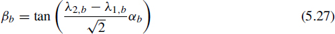
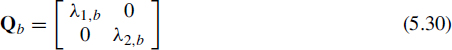
The variables λ_1,b and λ_2,b represent the relative amplitude of the two output signals with respect to the input and are given by:

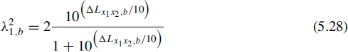
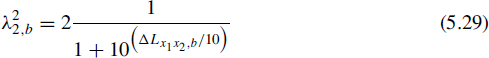
The corresponding ICLD synthesis matrix Q_b is then given by

Rotator ‘B’

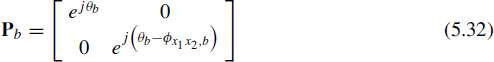
A second rotator type, rotator ‘B’, is based on a different decomposition of the mixing matrix. Rotator ‘B’ is applied when ICPD and OCPD parameters are present in the transmitted bitstream. For this rotator, the mixing matrix can be decomposed into three matrices P_b, A_b, V_b:

The diagonal matrix V_b enables real-valued (relative) scaling of the two orthogonal signals s_1,m and D(s_1,m). The matrix A_b is a real-valued rotation in the two-dimensional signal space, i.e., A⁻¹_b = A^T_b, and the diagonal matrix P_b enables modification of the complex-phase relationships between the output signals, hence |p_ij| = 1 for i = j and 0 otherwise.

The solution for the matrix Pb is given by:

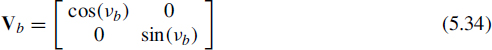
The matrices A_b and V_b can be interpreted as the eigenvector, eigenvalue decomposition of the covariance matrix of the (desired) output signals, assuming (optimum) phase alignment (P_b) prior to correlation. The solution for the eigenvectors and eigenvalues (maximizing the first eigenvalue v₁₁ and hence minimizing the energy of the decorrelated signal) results from a singular value decomposition (SVD) of the covariance matrix. The matrices A_b and V_b are given by (see [134] for more details):

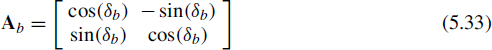
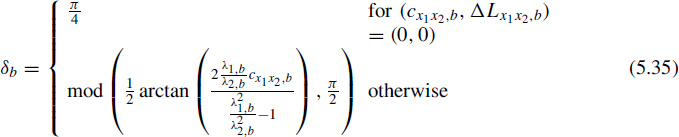
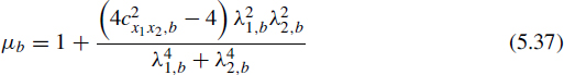
with δ_b being a rotation angle in the two-dimensional signal space defined by s_1,m and D(s_1,m), which is given by:

and ν_b a parameter for relative scaling of s_1,m and D(s_1,m) (i.e., the relation between the eigenvalues of the desired covariance matrix):

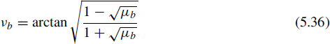
with

A visualization of this rotator is shown in Figure 5.10. The two (desired) output signals are shown along the horizontal and vertical axis. All sample pairs _{m,1 m,2} can be represented as points in the two-dimensional space (plane) shown in Figure 5.10. A large set of points form a oval-like shape. The size (in the vertical and horizontal direction) is determined by the variance (or power) of _m,1 and _m,2, respectively. Its orientation (the angle Δ) is dependent on the coherence between _m,1 and _m,2. The oval shape is decomposed into a dominant signal s_m,1 (the dominant component, having maximum power, which is equal to the square of the largest eigenvalue) and a residual signal D(s_m,1) (the residual component, with a power equal to the square of the smallest eigenvalue).

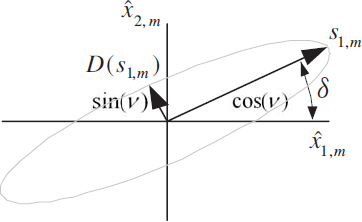
Figure 5.10 Visualization of rotator ‘B’.

It should be noted that a two-dimensional eigenvector problem has in principle four possible solutions: each eigenvector, which is represented as columns in the matrix A, may be multiplied with a factor −1. The modulo operator in Equation (5.35) ensures that the first eigenvector is always positioned in the first quadrant. This is very important to prevent sign changes of signal components across frames (which would lead to signal ‘dropouts’). However, this technique only works under the constraint of c_x1x2,b > 0, which is guaranteed if phase-alignment is applied. If no ICPD/OCPD parameters are transmitted, however, the ICC parameters may become negative, which hence requires rotator type ‘A’ since this rotator provides a stable solution for negative ICCs.

5.5.4 Interpolation

For each transmitted parameter the mixing matrix R_b is determined as described previously. However these matrices correspond in most cases to a single time instance, which depends on the segmentation and windowing procedure of the encoder. The sample index k at which a parameter set is valid is denoted by k_p, which is referred to as the parameter position. The parameter positions are transmitted from encoder to decoder along with the corresponding parameters themselves. For that particular QMF sample index (k = k_p), the mixing matrices R_b are determined as described previously. For QMF sample indices (k) in between parameter positions, the mixing matrices are interpolated linearly (i.e., its real and imaginary parts are interpolated individually). The interpolation of mixing matrices has the advantage that the decoder can process each ‘slot’ of hybrid QMF samples (i.e., one sample from each sub-band) one by one, without the need of storing a whole frame of sub-band samples in memory. This results in a significant memory reduction compared to frame-based synthesis methods.

The decoder-side interpolation is outlined in Figure 5.11. The top panel shows encoderside segmentation and windowing for a signal containing a transient.

The decoder is organized in frames. Each frame may contain one or more parameter sets, including corresponding parameter positions within the frame. By default, parameters are valid at the end of a frame, and for temporal positions for which no parameters are specified, the mixing matrices are interpolated linearly. This is indicated for the first three frames (0...2). For these frames, ‘normal’ analysis windows are applied in the encoder. The corresponding decoder parameter positions (k_p) coincide with the maximum (temporal center) of the analysis window. Frame ‘3’ contains a transient. The encoder applies a stop window that ends just before the transient. The corresponding decoder-side interpolation first ‘holds’ the parameters from frame ‘2’. A new parameter set and corresponding position (k_p(3)) is applied at a position that corresponds to the encoder-side transient window. These parameters are also valid for an extended range of sample indexes, corresponding to the size of the plateau of the encoder-side transient window. Frame ‘4’ again has a specified parameter position because this is the only parameter set transmitted for frame ‘4’, these parameters are valid until the end of the frame (since no interpolation can be performed because the parameters from frame ‘5’ are not known when processing frame ‘4’). Finally, frame ‘5’ is processed with default parameter positions at the end of the frame.

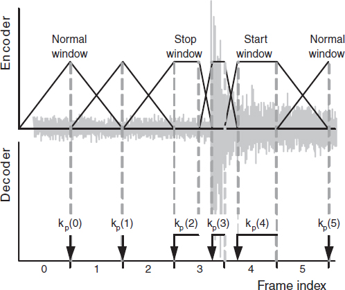
Figure 5.11 Encoder-side segmentation and windowing (top panel) and corresponding decoder– side parameter positions (lower panel).

5.5.5 Synthesis filterbanks

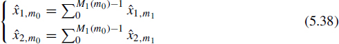
The mixing process is followed by a pair of hybrid QMF synthesis filterbanks (one for each output channel), which also consists of two stages (see Figure 5.4, right panel). The first stage comprises summation of the sub-sub-bands m₁ which stem from the same sub-band m₀:

Finally, up-sampling and convolution with synthesis filters (which are similar to the QMF analysis filters as specified by Equation 5.18) results in the final stereo output signal.

5.5.6 Parametric stereo in enhanced aacPlus

As described in the previous sections, enhanced aacPlus (or aacPlus v2) combines an AAC core codec with SBR and parametric stereo (PS). Since SBR and PS operate in virtually the same QMF domain, these parametric extensions can be combined in a very effective way, resulting in a significant complexity reduction compared to an operation mode where SBR and PS are both used independently. The structure of the enhanced aacPlus decoder is shown in Figure 5.12.

The incoming bitstream is demultiplexed into a (mono) AAC bitstream, SBR parameters and PS parameters. Subsequently, the AAC decoder generates a mono output signal of limited bandwidth. This signal is processed by a QMF analysis filterbank. The number of sub-bands amounts to 32, because of the limited signal bandwidth of the AAC decoder. The SBR process subsequently generates the upper half of the signal bandwidth, resulting in 64 sub-band signals. The delay of the SBR process amounts 6 QMF samples, which is exactly identical to the delay caused by the sub-filterbank of the hybrid QMF filter bank required for PS. In other words, the upper part (QMF band 32 to 63) of the signal (generated by SBR) can serve as direct input to the PS synthesis stage. The lower QMF bands (0 to 31) should only be processed by the sub-filterbank. In fact, the sub-filterbank only requires filtering in the first few QMF bands (see Table 5.3), while the remaining bands of the lower half of the bandwidth are simply delayed.

The resulting full-bandwidth hybrid QMF signal is processed by the parametric stereo decoder to generate two, full-bandwidth, hybrid QMF domain output signals. Finally, two hybrid QMF synthesis filter banks result in the two time-domain output signals.

To verify the compression gain resulting from parametric stereo, listening tests were conduced. The listening tests were carried out in two laboratories (indicated by black and gray in Figure 5.13) with 8 or 10 subjects, respectively. 10 test items from the MPEG4 aacPlus stereo verification test [141] were used as test material. The coded excerpts included aacPlus v1 using normal stereo coding operating at 24 and 32 kbps, as well as aacPlus v2 operating at 24 kbps total. Two lowpass anchors (with cutoff frequencies of 3.5 and 7 kHz) and a hidden reference were also included in the test. Subjects had to rate the perceptual quality of each codec in a MUSHRA test [148]. The tests were performed in a sound-proof listening room using headphones. Figure 5.13 shows subjective listening test results averaged across listeners per test lab. The horizontal axes indicates the audio codec; the vertical axis shows the corresponding MUSHRA score. Error bars denote the 95% confidence intervals.

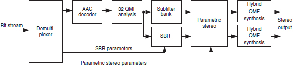
Figure 5.12 Structure of enhanced aacPlus (aacPlus v2).

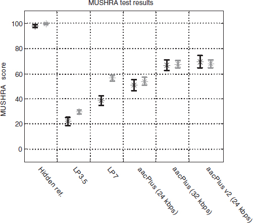
Figure 5.13 Subjective listening test results comparing aacPlus with aacPlus v2.

At both test sites, it was found that aacPlus v2 at 24 kbps achieves an average subjective quality that is equal to aacPlus v1 at 32 kbps, and is significantly better than aacPlus v1 at 24 kbps. In other words, parametric stereo results in an additional compression gain of 33% at bitrates in the range of 24–32 kb/s.