
Chapter 3
Scalability in the Frequency Domain
Tao generates one, one generates two, two generates three, three generates all things.
—Lao Dan (580–500 BC), Tao Te Ching
This chapter studies the problem of the scalability of the stability results for distributed control systems. The problem is closely related to some differential geometric properties of frequency response plots of local dynamics of agents (nodes) in networks, such as clockwise property, modulus monotonicity, slope monotonicity, phase velocity, critical point of clockwise property, etc. The chapter starts from the clockwise property which plays a key role in scalability analysis. Then, detailed geometric analysis of scalability is conducted for first-order and second-order time-delayed systems which are often encountered in coordinated control systems and end-to-end congestion control systems. Finally, based on the notion of convex directions in the space of stable quasi-polynomials, a frequency sweeping method of scalability test is provided for high-order time-delayed systems.
3.1 How the Scalability Condition is Related with Frequency Responses
Denote by γ the gain margin the transfer function
![]()
where W(s) is a rational function of s, and T > 0 is the delay constant. Actually, γ is defined by
(3.1) ![]()
where ωc > 0 is the minimal crossing frequency that satisfies the following equation
(3.2) ![]()
Note that the Nyquist plot of γW(jω)e−jωT crosses the real axis at (− 1, j0) when ω = ωc. We will call γW(s)e−Tsthe normalized transfer function of G(s) and denote it as ![]() .
.
Given n transfer functions ![]() , denote by
, denote by ![]() the normalized function of Gi(s). Consider a symmetric multi-agent system with Gi(s) as the transfer function of the ith agent. We have shown in the last chapter that the scalability condition for the system is
the normalized function of Gi(s). Consider a symmetric multi-agent system with Gi(s) as the transfer function of the ith agent. We have shown in the last chapter that the scalability condition for the system is
(3.3) ![]()
This condition requires us to check if the point (− 1, j0) is contained in the convex hull of ![]() and zero.
and zero.
The frequency response of the z-transfer function of a discrete-time system can also be denoted as ![]() , where the frequency variable ω takes values from the interval [− π, π]. To include the analysis of discrete-time systems in a unified framework, we denote the frequency interval as [ωa, ωb], and rewrite the scalability condition as
, where the frequency variable ω takes values from the interval [− π, π]. To include the analysis of discrete-time systems in a unified framework, we denote the frequency interval as [ωa, ωb], and rewrite the scalability condition as
The following lemma shows that it suffices to check the scalability condition for the boundary of the convex hull involved.
Lemma 3.1 Given normalized transfer functions ![]() , assume that
, assume that
and
Then, the scalability condition (3.4) holds if and only if
for all ![]() .
.
Proof. Note that (3.5) indicates that the condition (3.4) holds for ω = ω0. By continuity of the set ![]() on ω, the point (− 1, j0) enters
on ω, the point (− 1, j0) enters ![]() if and only if the boundary,
if and only if the boundary, ![]() , or κCo(0, Gi(ω)), passes through (− 1, j0). (3.6) has excluded the possibility that κCo(0, Gi(ω)) passes through (− 1, j0). Therefore, (3.4) holds if and only if (3.7) holds.
, or κCo(0, Gi(ω)), passes through (− 1, j0). (3.6) has excluded the possibility that κCo(0, Gi(ω)) passes through (− 1, j0). Therefore, (3.4) holds if and only if (3.7) holds. ![]()
Remark. In most cases condition (3.5) can be easily verified. For continuous-time systems, if Wi(s), ![]() , are proper, then
, are proper, then ![]() . Therefore,
. Therefore, ![]() and hence (3.5) holds. For discrete-time systems, to verify (3.5) we usually choose ω0 = π because
and hence (3.5) holds. For discrete-time systems, to verify (3.5) we usually choose ω0 = π because ![]() 's are real numbers. Condition (3.6) is ensured by the stability of the individual closed-loop system of each agent. When conditions (3.5) and (3.6) are satisfied, the scalability condition holds if and only if (− 1, j0) is not contained by the Nyquist plot of the convex combination of each pair of agents.
's are real numbers. Condition (3.6) is ensured by the stability of the individual closed-loop system of each agent. When conditions (3.5) and (3.6) are satisfied, the scalability condition holds if and only if (− 1, j0) is not contained by the Nyquist plot of the convex combination of each pair of agents.
Now, let us consider the following different cases.
Case 1: Homogeneous agents
In this case, the transfer functions of all the agents are assumed to be the same both in the rational part and in the delay unit, i.e.,
![]()
Obviously, for such a special case we have
![]()
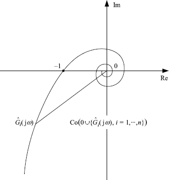
which is a line segment between the origin and any point at ![]() for a given frequency ω (see Figure 3.1). Obviously, in this case, the condition(3.4)holds if and only if the Nyquist plot of
for a given frequency ω (see Figure 3.1). Obviously, in this case, the condition(3.4)holds if and only if the Nyquist plot of![]() does not contain the point (− 1, j0).
does not contain the point (− 1, j0).
Figure 3.1 Homogeneous agents with identical delay.
Case 2: Heterogeneous agents with homogeneous frequency response
Let us consider the agents given by
![]()
If Ti ≠ Tj, for ![]() , the agents generally have different dynamics. However, if there exists a common transfer function
, the agents generally have different dynamics. However, if there exists a common transfer function ![]() such that for any given frequency
such that for any given frequency ![]() the following condition holds:
the following condition holds:
![]()
then all the agents have the same Nyquist plot which is delay-independent. For example, take ![]() . Then, for a given frequency ω0, all
. Then, for a given frequency ω0, all ![]() ,
, ![]() , are distributed at different points on the same plot
, are distributed at different points on the same plot ![]() . In this case, we are interested in the geometric property of
. In this case, we are interested in the geometric property of ![]() with which the following inclusion holds
with which the following inclusion holds
Obviously, if (3.8) holds, then, as shown by Figure 3.2, ![]() does not contain the point (− 1, j0) if
does not contain the point (− 1, j0) if ![]() does not contain (− 1, j0). Intuitively, the inclusion relationship (3.8) implies some “convexity” property of the Nyquist plot
does not contain (− 1, j0). Intuitively, the inclusion relationship (3.8) implies some “convexity” property of the Nyquist plot ![]() . Figure 3.3 gives an illustration that (3.8) may not hold when
. Figure 3.3 gives an illustration that (3.8) may not hold when ![]() does not have such convexity. In the next section we will study this property in detail.
does not have such convexity. In the next section we will study this property in detail.
Figure 3.2 Delay-independent frequency response: convex case.
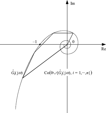
Figure 3.3 Delay-independent frequency response: non-convex case.
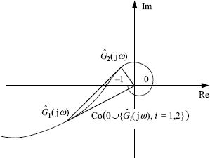
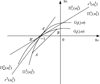
Case 3: Heterogeneous agents with heterogeneous frequency response
In this case, the scalability problem becomes much more complicated. Since all the agents have a different frequency response, we can only expect the following inclusion
Obviously, if (3.9) holds, then ![]() does not contain the point (− 1, j0) if each
does not contain the point (− 1, j0) if each ![]() does not contain (− 1, j0),
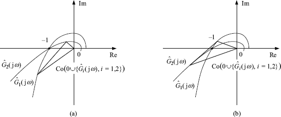
does not contain (− 1, j0), ![]() . However, even if the convexity is satisfied by each frequency response plot, (3.9) may hold as shown by Figure 3.4(a) or may not hold as shown by Figure 3.4(b).
. However, even if the convexity is satisfied by each frequency response plot, (3.9) may hold as shown by Figure 3.4(a) or may not hold as shown by Figure 3.4(b).
Figure 3.4 Heterogeneous frequency response.
3.2 Clockwise Property of Parameterized Curves
In this section we study the convexity of a smooth curve, which will be defined as a clockwise property. Let us first review some preliminary knowledge on the signed curvature of parameterized curves, which can be found in many textbooks of classic differential geometry such as Guggenheimer (1977).
Let Γ(t) be a curve in ![]() defined by two parametric equations:
defined by two parametric equations:
(3.10) ![]()
with X(t), Y(t) ![]() C2, which denotes the space of functions being two-times differentiable. The curvature
C2, which denotes the space of functions being two-times differentiable. The curvature ![]() of Γ at parameter t is defined as
of Γ at parameter t is defined as
where a superscript ' represents that a derivative operation is taken and subscripts denote the argument with respect to which derivatives are taken. Assume that ![]() exists for all t
exists for all t ![]() (tα, tβ), i.e., the denominator of (3.11) never vanishes in that interval.
(tα, tβ), i.e., the denominator of (3.11) never vanishes in that interval.
Let Γ be an image of the following complex function
(3.12) ![]()
in the complex plane. Then, from (3.11) it follows that the curvature of Γ can be also determined by (Gu (1994)
where G ' ω is the derivative of G(jω) with respect to ω, i.e., G ' ω = X ' ω + jY ' ω, G ” ωω is the derivative of G ' ω with respect to ω, ![]() and |G ' ω| are the conjugate and the module of G ' ω, respectively.
and |G ' ω| are the conjugate and the module of G ' ω, respectively.
Exercise 3.2 Derive (3.13) based on (3.11).
Now, let us introduce the notion of the clockwise property of a C2 curve.
Definition 3.3 The curve is said to be clockwise at t0 if ![]() . Conversely, the curve is anticlockwise at t0 if
. Conversely, the curve is anticlockwise at t0 if ![]() . If
. If ![]() holds for all t
holds for all t ![]() (tα, tβ) then Γ is said to be a clockwise curve.
(tα, tβ) then Γ is said to be a clockwise curve.
Geometrically, condition ![]() means that the center of curvature is on the right side of
means that the center of curvature is on the right side of ![]() , the tangent vector to Γ at Γ(t0) = (X(t0), Y(t0)), in other words, the vector
, the tangent vector to Γ at Γ(t0) = (X(t0), Y(t0)), in other words, the vector ![]() rotates clockwise (Figure 3.5).
rotates clockwise (Figure 3.5).
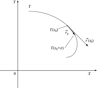
For any ε > 0, denote by ![]() the vector from the point Γ(t0) to the point Γ(t0 + ε) (Figure 3.5). For convenience of statement we define the positive direction of the tangent line at Γ(t0) as follows. The tangent vector
the vector from the point Γ(t0) to the point Γ(t0 + ε) (Figure 3.5). For convenience of statement we define the positive direction of the tangent line at Γ(t0) as follows. The tangent vector ![]() is said to point to the positive direction if the angle between
is said to point to the positive direction if the angle between ![]() and
and ![]() goes to zero when ε → 0. Otherwise,
goes to zero when ε → 0. Otherwise, ![]() is said to point to the negative direction if the angle between
is said to point to the negative direction if the angle between ![]() and
and ![]() goes to π when ε → 0.
goes to π when ε → 0.
Figure 3.5 Clockwise curve.
Then, we can split the tangent line r(t0) at Γ(t0) as follows:
![]()
where r+(t0) (r−(t0)) denotes the half of the tangent line r(t0) starting at Γ(t0) (not including Γ(t0)) in the positive (negative) direction (Figure 3.6).
Figure 3.6 Partition of a clockwise curve.
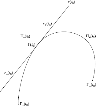
Accordingly, for any given t0 ![]() (tα, tβ), we can also split the curve Γ as follows (Figure 3.6):
(tα, tβ), we can also split the curve Γ as follows (Figure 3.6):
![]()
where Γ+(t0) (Γ−(t0)) denotes the part of the curve parameterized by t ![]() (t0, tβ] (t
(t0, tβ] (t ![]() [tα, t0)). Finally, we split the plane
[tα, t0)). Finally, we split the plane ![]() as follows
as follows
![]()
where Π+(t0) (Π−(t0)) is the open-half plane containing (not containing) the center of curvature of Γ at t0, assuming that ![]() .
.
The following lemma states how a clockwise curve enters and leaves the half plane Π+(t0).
Lemma 3.4 Suppose that the curve Γ is clockwise and does not admit self-intersections. Then, the following statements are true:
Proof. We only give the proof of statement (1). The proof of statement (2) is similar.
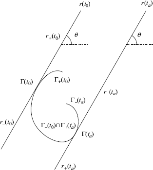
Assume that the phase of the tangent vector of Γ at t0 is Ψ(t0) = θ, and assume by contradiction that Γ(t![]() )
) ![]() r−(t0). Since Γ is clockwise, the phase, Ψ(t), of
r−(t0). Since Γ is clockwise, the phase, Ψ(t), of ![]() is strictly decreasing in t. Therefore, Ψ(t) > θ, ∀t < t0. So, we have
is strictly decreasing in t. Therefore, Ψ(t) > θ, ∀t < t0. So, we have
for some positive integer k![]() . Hence, there exists a ta
. Hence, there exists a ta ![]() (t
(t![]() , t0) such that Ψ(ta) = π + θ, i.e., the tangent line r(ta) is parallel to r(t0) (see Figure 3.7). Γ−(ta) can intersect r−(t0) without crossing r+(t0) and Γ−(t0) ∩ Γ+(ta) only if it crosses r−(ta) for some tb < ta (before crossing r+(ta)). By repeating the argument, it can be shown that Ψ(t
, t0) such that Ψ(ta) = π + θ, i.e., the tangent line r(ta) is parallel to r(t0) (see Figure 3.7). Γ−(ta) can intersect r−(t0) without crossing r+(t0) and Γ−(t0) ∩ Γ+(ta) only if it crosses r−(ta) for some tb < ta (before crossing r+(ta)). By repeating the argument, it can be shown that Ψ(t![]() ) > kπ + θ for any finite positive k which can be arbitrarily large. This contradicts (3.14) and hence, Γ(t
) > kπ + θ for any finite positive k which can be arbitrarily large. This contradicts (3.14) and hence, Γ(t![]() )
) ![]() r+(t0).
r+(t0). ![]()
Figure 3.7 Illustration of the proof of Lemma 3.4.
By Lemma 3.4, a clockwise curve having no self-intersections lies on one side of its tangent line if it neither crosses the half tangent line r+(t0) for t < t0 nor crosses the half tangent line r−(t0) for t > t0. For a curve lying on one side of its tangent line, the following lemma states that the convex hull of the curve together with the origin lies on one side of the tangent line if and only if the origin and the curve lie on the same side of the tangent line. This lemma addresses the concern of the second case given in the last section.
Lemma 3.5 Given t0 ![]() (tα, tβ) and
(tα, tβ) and ![]() , suppose
, suppose
(3.15) ![]()
Then,
(3.16) ![]()
holds for all κ ![]() [0, 1) if and only if 0
[0, 1) if and only if 0 ![]() Π+(t0).
Π+(t0).
Proof. Necessity is obvious. We just show sufficiency. Note that ![]() =
= ![]() . Since 0
. Since 0 ![]() Π+(t0) and Γ(ti)
Π+(t0) and Γ(ti) ![]() Π+(t0) ∪ Γ(t0), we have κΓ(ti)
Π+(t0) ∪ Γ(t0), we have κΓ(ti) ![]() Π+(t0) for all κ
Π+(t0) for all κ ![]() [0, 1). Now, all κΓ(ti)s,
[0, 1). Now, all κΓ(ti)s, ![]() together with the origin are inside Π+(t0), by the separation principle of the convex analysis,
together with the origin are inside Π+(t0), by the separation principle of the convex analysis,
![]()
for all κ ![]() [0, 1).
[0, 1). ![]()
For the convex combination of two curves we have the following lemma.
Lemma 3.6 Consider two curves Γ1(t) and Γ2(t) with t ![]() [tα, tβ]. Suppose Γ1(t) and Γ2(t) intersect with each other at the point (− 1, 0) with parameters
[tα, tβ]. Suppose Γ1(t) and Γ2(t) intersect with each other at the point (− 1, 0) with parameters ![]() and
and ![]() , respectively, i.e.,
, respectively, i.e.,
(3.17) ![]()
Then,
holds for all t ![]() [tα, tβ] if
[tα, tβ] if
![]()
or
![]()
for all t ![]() [tα, tβ].
[tα, tβ].
Proof. For any fixed t ![]() [tα, tβ], Γ1(t) and Γ2(t) simultaneously lie on the right side of the tangent line
[tα, tβ], Γ1(t) and Γ2(t) simultaneously lie on the right side of the tangent line ![]() or on the right side of
or on the right side of ![]() . Therefore, for any t
. Therefore, for any t ![]() [tα, tβ], we have
[tα, tβ], we have
![]()
or
![]()
for 0 ≤ κ < 1, which implies (3.18). ![]()
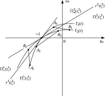
Lemma 3.6 is illustrated by Figure 3.8, where segments AiBi, i = 1, 2, 3, represent possible cases of Co(Γ1(t), Γ2(t)) for different values of parameter t.
Figure 3.8 Illustration of Lemma 3.6
3.3 Scalability of First-Order Systems
In this section we study some global differential geometric properties of the Nyquist plot of the transfer function of the first-order time-delayed system with a single (open-loop) integrator. Many dynamic nodes in distributed control systems, such as the primal or dual algorithm of the congestion control of communication networks, ideal mobile agents (i.e., mobile agents without inertia), can be modeled by this kind of transfer function.
3.3.1 Continuous-Time System
Consider the transfer function
where T > 0 is the delay constant, and k > 0 is the gain. The frequency response of the system is
(3.22) ![]()
Proposition 3.7 The Nyquist plot G(jω) of system (3.19) is clockwise in the parameter interval (0, ∞).
Proof. From (3.20) it is easy to get
It follows that
![]()
Therefore
![]()
By Definition 3.3 this implies that G(jω) is clockwise for all ω ![]() (0, ∞).
(0, ∞). ![]()
Proposition 3.8 The Nyquist plot G(jω) of system (3.19) has no self-intersection in the parameter interval (0, ∞).
Proof. The proposition is obvious from the fact that the modulus of the frequency response (see (3.20)) is strictly decreasing with respect to ω in the interval (0, ∞). ![]()
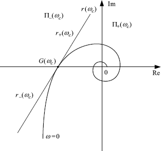
Let ωc be the minimal crossing frequency of G(jω), i.e., the Nyquist plot of G(jω) crosses the real axis for the first time at ω = ωc as ω varies from 0 to ∞. It is easy to get
(3.23) ![]()
for system (3.19). According to (3.21), straightforward calculation shows that the slope of r(ωc), the tangent line to G(jω) at G(jωc), is
(3.24) ![]()
which is independent of the delay constant T. Therefore, the angle Ψc between the line r+(ωc) and the real axis of the complex plane satisfies
Lemma 3.9 For all ω ![]() [0, ∞), the Nyquist plot of system (3.19) lies on the right side of the tangent line to G(jω) at G(jωc), denoted by r(ωc), i.e., G(jω)
[0, ∞), the Nyquist plot of system (3.19) lies on the right side of the tangent line to G(jω) at G(jωc), denoted by r(ωc), i.e., G(jω) ![]() G(jωc) ∪ Π+(ωc), ∀ω
G(jωc) ∪ Π+(ωc), ∀ω ![]() [0, ∞).
[0, ∞).
Proof. Firstly, we prove the lemma for all ω ![]() (0, ∞). By Proposition 3.7 and Proposition 3.8, the Nyquist plot of system (3.19) is clockwise and has no self-intersection in the parameter interval (0, ∞). Therefore, by Lemma 3.4, the only way that the curve G+(jωc) can leave the half plane Π+(ωc) is by crossing the line r−(ωc) and the only way that G−(ωc) can enter the half plane Π+(ωc) is by crossing the line r+(ωc). Inequality (3.25) implies that the modulus of any point on r−(ωc) is greater than |G(jωc)|. However, the modulus of the frequency response,
(0, ∞). By Proposition 3.7 and Proposition 3.8, the Nyquist plot of system (3.19) is clockwise and has no self-intersection in the parameter interval (0, ∞). Therefore, by Lemma 3.4, the only way that the curve G+(jωc) can leave the half plane Π+(ωc) is by crossing the line r−(ωc) and the only way that G−(ωc) can enter the half plane Π+(ωc) is by crossing the line r+(ωc). Inequality (3.25) implies that the modulus of any point on r−(ωc) is greater than |G(jωc)|. However, the modulus of the frequency response, ![]() , is strictly decreasing in the interval (0, ∞) and hence, |G(jω)| < |G(jωc)|, ∀ω
, is strictly decreasing in the interval (0, ∞) and hence, |G(jω)| < |G(jωc)|, ∀ω ![]() (ωc, ∞). Therefore, it is impossible that the curve Γ+(ωc) crosses the line r−(ωc) for all ω
(ωc, ∞). Therefore, it is impossible that the curve Γ+(ωc) crosses the line r−(ωc) for all ω ![]() (ωc, ∞). On the other hand, from (<xreftarget = " c03− mdis − 0033 "/>) we know that for all ω
(ωc, ∞). On the other hand, from (<xreftarget = " c03− mdis − 0033 "/>) we know that for all ω ![]() (0, ωc) the phase of G(jω) is in the interval
(0, ωc) the phase of G(jω) is in the interval ![]() , i.e., the curve G−(jωc) lies inside the third quadrant of the complex plane and hence cannot cross the line r+(ωc) which is above the real axis of the complex plane. Hence, we have proved G(jω)
, i.e., the curve G−(jωc) lies inside the third quadrant of the complex plane and hence cannot cross the line r+(ωc) which is above the real axis of the complex plane. Hence, we have proved G(jω) ![]() G(jωc) ∪ Π+(ωc), for all ω
G(jωc) ∪ Π+(ωc), for all ω ![]() (0, ∞).
(0, ∞).
When ω → 0, we can write G(jω) as
(3.26) ![]()
where ε is an infinitely small positive number and θ ![]() [0, π/2]. When θ varies from 0 to π/2, G(jω) draws a clockwise infinitely large quarter-circle with phase angle in [− π/2, 0]. So it is also in Π+(ωc).
[0, π/2]. When θ varies from 0 to π/2, G(jω) draws a clockwise infinitely large quarter-circle with phase angle in [− π/2, 0]. So it is also in Π+(ωc). ![]()
Now we are ready to prove the following theorem.
Theorem 3.10 For any given natural number n ≥ 2, let
(3.27) ![]()
where
and ![]() , are divers nonnegative delay constants. Then
, are divers nonnegative delay constants. Then ![]() does not contain the point (− 1, j0) for all κ
does not contain the point (− 1, j0) for all κ ![]() [0, 1) and all ω
[0, 1) and all ω ![]() (− ∞, ∞).
(− ∞, ∞).
Proof. By the symmetry property of the frequency response we need only to prove the theorem for all ω ![]() [0, ∞).
[0, ∞).
Let
Obviously, (3.29) forms an onto map from ω ![]() [0, ∞) to xi
[0, ∞) to xi ![]() [0, ∞). We notice that under the given gain condition (3.28),
[0, ∞). We notice that under the given gain condition (3.28), ![]() . Therefore, all of the Nyquist plots of
. Therefore, all of the Nyquist plots of ![]() , share a common curve, i.e.,
, share a common curve, i.e., ![]() , on the complex plane. And the curve crosses the real axis for the first time at the point (− 1, j0). By Lemma 3.9 we have G(jx)
, on the complex plane. And the curve crosses the real axis for the first time at the point (− 1, j0). By Lemma 3.9 we have G(jx) ![]() (− 1, j0) ∪ Π+(− 1, j0), ∀x
(− 1, j0) ∪ Π+(− 1, j0), ∀x ![]() [0, ∞). For any given ω
[0, ∞). For any given ω ![]() [0, ∞) we have xi = Tiω
[0, ∞) we have xi = Tiω ![]() [0, ∞). So it follows that
[0, ∞). So it follows that
(3.30) ![]()
By Lemma 3.5 we know that
(3.31) ![]()
holds for all κ ![]() [0, 1). Therefore
[0, 1). Therefore ![]() does not contain the point (− 1, j0) for all κ
does not contain the point (− 1, j0) for all κ ![]() [0, 1) and all ω
[0, 1) and all ω ![]() [0, ∞) because (− 1, j0) ∉ Π+(− 1, j0).
[0, ∞) because (− 1, j0) ∉ Π+(− 1, j0). ![]()
3.3.2 Discrete-Time System
For a discrete-time system the frequency response is the value of its z-transfer function at the unit circle, namely, G(ejω), ω ![]() (− π, π]. For simplicity of notation we will write G(ejω) as G(ω) for discrete-time systems. Let us study the first-order time-delayed system
(− π, π]. For simplicity of notation we will write G(ejω) as G(ω) for discrete-time systems. Let us study the first-order time-delayed system
where D is a positive integer representing the delay, and k > 0 is the gain. This is a discrete-time analogue of system (3.19). Along the modified unit circle the frequency response of system (3.32) is
(3.33) ![]()
(3.36) ![]()
Since G(z) has a pole z = 1 on the unit circle, we should modify the unit circle by adding a small half-circle around the pole z = 1 (see Figure 2.13). In this way the pole can be considered as inside the unit circle. The Nyquist plot of G(ω) will go to infinity when ω → 0 and draw a half-circle with an infinite radius clockwise.
Proposition 3.11 The Nyquist plot of system G(ω) (3.32) is clockwise in the parameter interval [0, π].
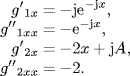
Proof. Without loss of generality we suppose that k = 1 in (3.32). To prove the proposition we need to consider only the sign of the numerator of the curvature. By (3.13) we have
![]()
Straightforward calculating yields
Therefore, we have
![]()
which implies
![]()
So, the clockwise property of the Nyquist plot of (3.32) is proved. ![]()
Proposition 3.12 The Nyquist plot G(ω) of system (3.32) has no self-intersection in the parameter interval (0, π].
Proof. The proposition is obvious from the fact that the modulus of the frequency response (see (3.34)), ![]() , is strictly decreasing in the interval (0, π].
, is strictly decreasing in the interval (0, π]. ![]()
Let ωc be the frequency at which the Nyquist plot Γ(ω) intersects the real axis for the first time as ω varies from 0 to π. It is easy to get
(3.37) ![]()
for system (3.32). From (3.35), straightforward calculation shows that the slope of r(ωc), the tangent line to G(ω) at G(ωc), is
It is always the case that kc > 0 as D is a delay constant which is a nonnegative integer for discrete-time systems. Therefore, the angle Ψc between the line r+(ωc) and the real axis of the complex plane satisfies
Proposition 3.13 For all ω ![]() (0, π], the Nyquist plot G(ω) of system (3.19) lies on the right side of r(ωc), i.e., G(ω)
(0, π], the Nyquist plot G(ω) of system (3.19) lies on the right side of r(ωc), i.e., G(ω) ![]() G(ωc) ∪ Π+(ωc), ∀ω
G(ωc) ∪ Π+(ωc), ∀ω ![]() (0, π].
(0, π].
Proof. By Proposition 3.11 and Proposition 3.12, the Nyquist plot G(ω) of system (3.32) is clockwise and has no self-intersection in the parameter interval [0, π]. Therefore, by Lemma 3.4, the only way that the curve G+(ωc) can leave the half plane Π+(ωc) is by crossing the line r−(ωc) and the only way that G−(ωc) can enter the half plane Π+(ωc) is by crossing the line r+(ωc) (see Figure 3.9). Equation (3.34) shows that the modulus of the frequency response, ![]() , is strictly decreasing in the interval (0, π] and hence, |G(ω)| < |G(ωc)|, ∀ω
, is strictly decreasing in the interval (0, π] and hence, |G(ω)| < |G(ωc)|, ∀ω ![]() (ωc, π]. But inequality (3.39) implies that the modulus of any point on r−(ωc) is greater than |G(ωc)|. Therefore, it is impossible that the curve G+(ωc) crosses the line r−(ωc) for all ω
(ωc, π]. But inequality (3.39) implies that the modulus of any point on r−(ωc) is greater than |G(ωc)|. Therefore, it is impossible that the curve G+(ωc) crosses the line r−(ωc) for all ω ![]() (ωc, π]. On the other hand, from (3.34) we know that for all ω
(ωc, π]. On the other hand, from (3.34) we know that for all ω ![]() (0, ωc) the phase of G(ω) is in the interval
(0, ωc) the phase of G(ω) is in the interval ![]() , i.e., the curve G−(ωc) lies inside the third quadrant of the complex plane and hence cannot cross the line r+(ωc) which is above the real axis of the complex plane.
, i.e., the curve G−(ωc) lies inside the third quadrant of the complex plane and hence cannot cross the line r+(ωc) which is above the real axis of the complex plane. ![]()
Figure 3.9 Proposition 3.13
Now, let us consider the Nyquist plots of two systems of the same form with different delay constants
where
It is not difficult to verify that both of the plots cross the real axis for the first time at the same point (− 1, j0) with the crossing frequencies as
Let ![]() and
and ![]() be slopes of tangent lines to G1(ω) and G2(ω) at the point (− 1, j0) respectively. It is easy to show that kc given by (3.38) is strictly decreasing in the delay constant D. Therefore, we have the following proposition.
be slopes of tangent lines to G1(ω) and G2(ω) at the point (− 1, j0) respectively. It is easy to show that kc given by (3.38) is strictly decreasing in the delay constant D. Therefore, we have the following proposition.
Proposition 3.14 For frequency responses given by (3.40) and (3.41) the following inequality holds:
(3.43) ![]()
Lemma 3.15 Let Gi(ω), i = 1, 2 be given by (3.40) and (3.41). Then,
holds for all ω ![]() [− π, π] and 0 ≤ κ < 1.
[− π, π] and 0 ≤ κ < 1.
Proof. First of all, we note that both G1(ω) and G2(ω) enjoy the symmetry property with respect to the real axis of the complex plane, i.e.,
![]()
Thus, we need only to prove (3.44) for all ω ![]() [0, π]. Without loss of generality, we assume that D2 < D1. Then we have
[0, π]. Without loss of generality, we assume that D2 < D1. Then we have ![]() by (3.42). Now, let us split the frequency interval [0, π] into four parts, namely
by (3.42). Now, let us split the frequency interval [0, π] into four parts, namely ![]() ,
, ![]() and
and ![]() , and consider each case below.
, and consider each case below.
Figure 3.10 Illustration of proof of Lemma 3.15.
In this case we can write G1(ω) and G2(ω) as
where ε is an infinitely small positive number and θ ![]() [0, π/2]. So delays play no role when ω → 0. When θ varies from 0 to π/2 Both G1(ω) and G2(ω) synchronously draw a clockwise infinitely large quarter-circle with phase angle in [− π/2, 0]. Hence,
[0, π/2]. So delays play no role when ω → 0. When θ varies from 0 to π/2 Both G1(ω) and G2(ω) synchronously draw a clockwise infinitely large quarter-circle with phase angle in [− π/2, 0]. Hence, ![]() in this case.
in this case.
Summarizing all the four cases we know
![]()
or
![]()
for any ω ![]() [0, π]. By Lemma 3.6, we conclude that
[0, π]. By Lemma 3.6, we conclude that
![]()
holds for all ω ![]() [0, π] and 0 ≤ κ < 1.
[0, π] and 0 ≤ κ < 1. ![]()
Now, we are ready to prove the following theorem.
Theorem 3.16 Given any natural number n ≥ 2,
(3.45) ![]()
holds for all κ ![]() [0, 1) and all ω
[0, 1) and all ω ![]() (− π, π), where
(− π, π), where
where ![]() , are divers nonnegative integers. Consequently,
, are divers nonnegative integers. Consequently, ![]() does not contain the point (− 1, j0) for all ω
does not contain the point (− 1, j0) for all ω ![]() [− π, π] and all κ
[− π, π] and all κ ![]() [0, 1).
[0, 1).
Proof. By the symmetry property of the frequency response we need only to prove the lemma for all ω ![]() [0, π].
[0, π].
We first note that
holds for all ω ![]() [0, π] since both Gi(ω) and the origin of the complex plane lie in
[0, π] since both Gi(ω) and the origin of the complex plane lie in ![]() . We also note that
. We also note that
![]()
holds for ω = π since Gi(π) = − cos (Diπ)/2 > − 1. Then, by continuity of the set ![]() on ω,
on ω, ![]() goes out of the region
goes out of the region ![]() implies its boundary,
implies its boundary, ![]() , or κCo{0, Gi(ω)}, goes out of the same region. But Lemma 3.15 and (3.46) have excluded this possibility. Therefore, we conclude that
, or κCo{0, Gi(ω)}, goes out of the same region. But Lemma 3.15 and (3.46) have excluded this possibility. Therefore, we conclude that
![]()
for all ω ![]() [− π, π]. Therefore,
[− π, π]. Therefore, ![]() does not contain the point (− 1, j0) for all ω
does not contain the point (− 1, j0) for all ω ![]() [− π, π] because
[− π, π] because ![]() .
. ![]()
3.4 Scalability of Second-Order Systems
In this section we study the second-order time-delayed systems of two types. In accordance with textbooks on classic control theory, it will be called a system of type I if its (open-loop) transfer function contains a single integrator, or a system of type II if its transfer function contains double integrators.
3.4.1 System of Type I
Many dynamic nodes of distributed control systems, such as the primal-dual algorithm of the congestion control of communication networks, and position feedback control of a mobile agent with inertia, can be modeled as a second-order system with a single integrator. The time-delayed form of such a system is given by
where k > 0 is the gain, T > 0 is the delay constant, and −α < 0 is the LHP pole of the system.
The frequency response of system (3.47) is given by
(3.48) ![]()
Denote by ωc > 0 the minimal crossing frequency of G(jω), i.e., G(jω) crosses the real axis of the complex plane for the first time when ω = ωc. Actually, ωc > 0 is the minimal frequency satisfying the following equation:
Denote by γ the gain margin of G(s), which is defined by
(3.50) ![]()
From (3.49) we have
![]()
Using this equality, we get
(3.51) 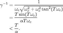
Now, let
(3.52) ![]()
(3.53) ![]()
Then, G(jω) can be rewritten as
(3.54) ![]()
by abusing the notation G(·) just for convenience. Obviously, for a given system G(s), the curve
(3.55) ![]()
is just a linear zoom of the Nyquist plot of G(jω) and hence preserves almost all of the geometric properties of G(jω). For example, the Nyquist plot of G(jω) is clockwise in the frequency interval [ω1, ω2] if and only if the curve of G(jx) is clockwise in the parameter interval [Tω1, Tω2]. Similarly, G(jω) does not admit self-intersection in the interval [ω1, ω2] if and only if G(jx) does not admit self-intersections in the interval [Tω1, Tω2].
Proposition 3.17 The curve G(jx) does not admit self-intersections for all x ≥ 0.
Proof. The assertion is obvious from the fact that the modulus of G(jx), i.e.,
![]()
is strictly decreasing in x in the interval [0, ∞). ![]()
Proposition 3.18 The curve G(jx) is clockwise in the parameter interval [0, ∞).
Proof. To prove the proposition, we only need to check the sign of the numerator of the curvature. By (3.13) we know that the curvature of G(jx) is given by
![]()
Denote
![]()
where
Then, we have
Therefore,
Straightforward calculation yields
(3.59) ![]()
Taking (3.58) into account, we get
(3.60) ![]()
From (3.56) and (3.57), we get
So, we have
![]()
where
(3.61) ![]()
Therefore,
where
Obviously, Im(QP*) < 0, for all x > 0 and all A ≥ 0. This implies
![]()
Thus, the clockwise property of the curve of G(jx) in the interval [0, ∞) is proved. ![]()
Given ωc the minimal crossing frequency of G(jω), it is obvious that G(jx) crosses the real axis of the complex plane for the first time when
(3.65) ![]()
According to (3.49), the minimal crossing parameter xc satisfies
Differentiating both sides of the above equation with respect to A, we get
![]()
which gives
where ![]() . So, we have the following proposition.
. So, we have the following proposition.
Proposition 3.19 The minimal crossing point xc is a strictly monotonically increasing function of parameter A.
Denote by r(xc) the tangent line of G(jx) at the minimal crossing point xc. Then, we can prove the following result.
Proposition 3.20 The slope of r(xc), denoted by Tc, is a strictly monotonically increasing function of parameter A. Moreover, Tc > 0 for all A > 0.
Proof. The slope of the tangent line r(xc) is given by
(3.68) ![]()
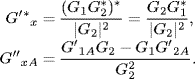
Note that
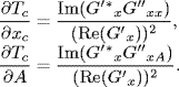
So, we get
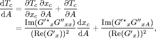
where ![]() has been obtained in the proof of Proposition 3.18 (see (3.63) and (3.64)), and
has been obtained in the proof of Proposition 3.18 (see (3.63) and (3.64)), and ![]() is given by (3.67). Now, we calculate
is given by (3.67). Now, we calculate ![]() . Denote
. Denote
![]()
where g1(x) and g2(x) are given by (3.56) and (3.57), respectively. Then, we have
Therefore,
Straightforward calculation yields
![]()
Taking (3.70) into account, we get
![]()
From (3.56) and (3.57), we get
![]()
So, we have
![]()
where
![]()
and P is given by (3.62). Therefore,
where
Now, substituting (3.67), (3.63), (3.64), (3.72) and (3.73) into (3.69) yields
![]()
where
![]()
Therefore, Tc(A) is a strictly monotonically increasing function of the parameter A. Finally, we note that Tc = 0 when A = 0. This implies that Tc > 0 for all A > 0. The proposition is thus proved. ![]()
Now, using Lemma 3.4, we can prove the following result.
Proposition 3.21 For all x ![]() [0, ∞), the curve G(jx) lies on the right side of r(xc), i.e., G(jx)
[0, ∞), the curve G(jx) lies on the right side of r(xc), i.e., G(jx) ![]() G(jxc) ∪ Π+(xc), ∀x
G(jxc) ∪ Π+(xc), ∀x ![]() [0, ∞).
[0, ∞).
Proof. For simplicity of statement, we denote the curve of G(jx) in the parameter interval [0, ∞) as G[0, ∞). Also, we denote the curve G(jx) in the parameter interval (xc, ∞) as G+(xc) and the curve G(jx) in the parameter interval [0, xc) as G−(xc). By Proposition 3.17 and Proposition 3.18, G[0, ∞) is clockwise and has no self-intersections. Therefore, by Lemma 3.4, the only way that the curve G+(xc) can leave the half plane Π+(xc) is by crossing the line r−(xc) and the only way that G−(xc) can enter the half plane Π+(ωc) is by crossing the line r+(ωc). In the proof of Proposition 3.17, we have mentioned that the modulus |G(jx)| is strictly decreasing in x, and hence, |G(jx)| < |G(jxc)|, ∀x ![]() (xc, ∞). But, from Proposition 3.20, we know that the slope of the tangent line at x = xc is greater than zero. This implies that the modulus of any point on r−(xc) is greater than |G(jxc)|. Therefore, it is impossible that the curve G+(xc) crosses the line r−(xc) for all x
(xc, ∞). But, from Proposition 3.20, we know that the slope of the tangent line at x = xc is greater than zero. This implies that the modulus of any point on r−(xc) is greater than |G(jxc)|. Therefore, it is impossible that the curve G+(xc) crosses the line r−(xc) for all x ![]() (xc, ∞). On the other hand, for any x
(xc, ∞). On the other hand, for any x ![]() [0, xc), the curve G−(xc) lies inside the third quadrant of the complex plane and hence cannot cross the line r+(xc), which is located above the real axis of the complex plane. The proposition is thus proved.
[0, xc), the curve G−(xc) lies inside the third quadrant of the complex plane and hence cannot cross the line r+(xc), which is located above the real axis of the complex plane. The proposition is thus proved. ![]()
Next, let us consider the Nyquist plots of two systems of the same form with different delay constants:
where γi is the gain margin of the transfer function
![]()
Lemma 3.22 If the following condition
holds for the frequency responses of systems given by (3.74), then
(3.76) ![]()
holds for all real numbers κ ![]() [0, 1) and all ω
[0, 1) and all ω ![]() [0, ∞).
[0, ∞).
Proof. First of all, we note that both of the two plots of the functions in the form (3.74) cross the real axis for the first time at the same point (− 1, j0), with minimal crossing frequencies
(3.77) ![]()
where ![]() is given by (3.66). Without loss of generality, assume that A1 < A2, which by (3.75) also implies that
is given by (3.66). Without loss of generality, assume that A1 < A2, which by (3.75) also implies that
![]()
Since when ![]() both G1(jω) and G2(jω) are in the third quadrant, the conclusion of the lemma obviously holds in the frequency interval
both G1(jω) and G2(jω) are in the third quadrant, the conclusion of the lemma obviously holds in the frequency interval ![]() . We need to prove the proposition for the frequency interval
. We need to prove the proposition for the frequency interval ![]() . To do so, let us split this frequency interval into two parts, namely
. To do so, let us split this frequency interval into two parts, namely ![]() and
and ![]() . We consider each case below.
. We consider each case below.
Summarizing the conclusion obtained in the above two cases, we complete the proof of the lemma. ![]()
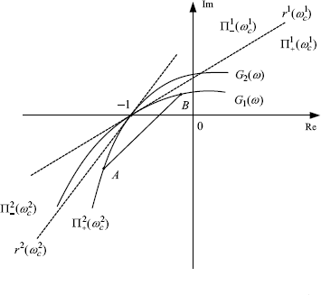
A graphical illustration of Lemma 3.22 is given by Figure 3.11. Note that condition (3.75) is necessary for the conclusion of Lemma 3.22 Otherwise, the less curved G2(jω) may cross the real axis and enter the second quadrant before the more curved G1(jω) does. In this case, Co(G1(jω), G2(jω)) will be out of the region ![]() , as illustrated as A ' B ' in Figure 3.11.
, as illustrated as A ' B ' in Figure 3.11.
Figure 3.11 Illustration of Lemma 3.22
Now, we are ready to prove the following theorem.
Theorem 3.23 Suppose that the following condition
(3.78) ![]()
holds for the frequency response of a family of systems described by
where γi is the gain margin of the transfer function
![]()
Then, ![]() does not contain the point (− 1, j0) for all real numbers κ
does not contain the point (− 1, j0) for all real numbers κ ![]() [0, 1) and all ω
[0, 1) and all ω ![]() [0, ∞).
[0, ∞).
Proof. By Lemma 3.22, we know that
holds for all ![]() . Note that
. Note that
holds for all ω ![]() [0, ∞) since both Gi(jω) and the origin of the complex plane lie in
[0, ∞) since both Gi(jω) and the origin of the complex plane lie in ![]() . Also, note that
. Also, note that
![]()
holds when ω→ ∞ since Gi(j ∞) goes to the origin of the complex plane for all ![]() . Therefore, by continuity of the set
. Therefore, by continuity of the set ![]() on ω, if
on ω, if ![]() goes out of the region
goes out of the region ![]() , then its boundary,
, then its boundary,
![]()
or
![]()
will go out of the same region at some frequency. But (3.80) and (3.81) have excluded this possibility. Therefore, we conclude that
![]()
Since ![]() ,
, ![]() does not contain the point (− 1, j0) for all ω
does not contain the point (− 1, j0) for all ω ![]() [0, ∞). The theorem is thus proved.
[0, ∞). The theorem is thus proved. ![]()
For the family of systems given by (3.79), denote by ![]() the index of the system with minimal value of parameter Ai, i.e.,
the index of the system with minimal value of parameter Ai, i.e.,
(3.82) ![]()
Let ![]() be the slope of the tangent line to the Nyquist plot of
be the slope of the tangent line to the Nyquist plot of ![]() at the intersection point C, as illustrated by Figure 3.12. It is easy to see that
at the intersection point C, as illustrated by Figure 3.12. It is easy to see that ![]() . An analytic formula of
. An analytic formula of ![]() is given by
is given by
(3.83) ![]()
Define
Now, we are ready to give an alternative theorem for checking if (− 1, j0) is contained by ![]() .
.
Figure 3.12 Definition of μi and illustration of the proof of Theorem 3.24.
Theorem 3.24 Let μi be defined by (3.84) and Gi(jω) be defined by (3.79). Then, ![]() does not contain the point (− 1, j0) for all real numbers κ
does not contain the point (− 1, j0) for all real numbers κ ![]() [0, 1) and all ω
[0, 1) and all ω ![]() [0, ∞).
[0, ∞).
Proof. For simplicity, we only show the validity of the theorem for the case of two systems. But the proof can be directly extended to the general case.
Without loss of generality, assume A1 < A2, i.e., ![]() . Then, we have μ1 = 1 and
. Then, we have μ1 = 1 and
![]()
where ![]() is the slope of the tangent line
is the slope of the tangent line ![]() (see Figure 3.12). To prove the theorem, it suffices to show that
(see Figure 3.12). To prove the theorem, it suffices to show that ![]() .
.
Note that G1(jω) intersects the real axis of the complex plane at (− 1, j0) while μ2G2(jω) intersects the real axis at point F with coordinate (μ2, j0). It is easy to see that |OF| = |OE| = μ2, where |OE| is the shortest distance to the origin from the tangent line ![]() . Since the modulus of μ2G2(jω) is strictly monotonically decreasing in ω, we have
. Since the modulus of μ2G2(jω) is strictly monotonically decreasing in ω, we have
![]()
which implies that μ2G2(jω) never touches ![]() for
for ![]() . To show that μ2G2(jω) never touches
. To show that μ2G2(jω) never touches ![]() for
for ![]() , we only need to notice the fact that μ2 < 1 and
, we only need to notice the fact that μ2 < 1 and ![]() (by Proposition 3.20), where
(by Proposition 3.20), where ![]() and
and ![]() are the slopes of the tangent lines
are the slopes of the tangent lines ![]() and
and ![]() , respectively (see Figure 3.12).
, respectively (see Figure 3.12). ![]()
3.4.2 System of Type II
Many dynamic nodes in distributed control systems, such as the second-order active queue management (AQM) algorithm, force-controlled ideal mobile agents with both position and velocity feedback, can be modeled as a second-order system with double integrators, which is referred to as the second-order system of type II in the literature of classic feedback control. In this subsection, we give detailed analysis of the geometric properties of the frequency response of the time-delayed system
where k > 0 is the gain, T > 0 is the delay constant, and −α < 0 is the zero of the system. The frequency response of system (3.85) is
(3.86) ![]()
Let x = Tω. Then, G(jω) can be rewritten as
where
(3.88) ![]()
is a key parameter in the geometric analysis for this system. (3.87) shows that for a given system G(s), the curve
(3.89) ![]()
is just a linear zoom of the Nyquist plot of G(jω). Hence, G(jx) preserves all of the geometric properties of G(jω). For example, the Nyquist plot of G(jω) is clockwise in the frequency interval [ω1, ω2] if and only if the curve of G(jx) is clockwise in the parameter interval [Tω1, Tω2]. Similarly, G(jω) does not admit self-intersection in the interval [ω1, ω2] if and only if G(jx) does not admit self-intersections in the interval [Tω1, Tω2]. Therefore, next we will mainly study the geometric property of G(jx) instead of G(jω).
Proposition 3.25 The curve G(jx) does not admit self-intersections for all x ≥ 0.
Proof. The proposition is obvious from the fact that the modulus of G(jx), i.e.,
![]()
is strictly decreasing in x in the interval [0, ∞). ![]()
Proposition 3.26 If A < 1, then the curve G(jx) is clockwise in the parameter interval [x0, ∞), where
Proof. To prove the proposition we only need to check the sign of the numerator of the curvature
![]()
Straightforward calculating yields
(3.92) ![]()
(3.93) ![]()
Therefore,
Denote
When 0 ≤ A ≤ 1, it is easy to get the largest root of p(x) as
(3.96) ![]()
When x > x0 we have p(x) > 0. This implies
![]()
So, the clockwise property of the curve of G(jx) in the interval [x0, ∞) is proved. ![]()
We call x0 the maximal critical parameter of G(jx), and correspondingly, ω0 = x0/T the maximal critical frequency of G(jω).
Let ωc be the minimal crossing frequency of G(jω), i.e, the Nyquist plot of G(jω) crosses the real axis for the first time at ω = ωc as ω varies from 0 to ∞. It is easy to prove that ωc is the minimal frequency satisfying
Similarly, we have the minimal crossing parameter of G(jx) at
![]()
According to (3.97), the minimal crossing point xc satisfies
Both x0 and xc can be regarded as functions of A, an adjustable parameter. The following proposition gives some important properties of x0(A) and xc(A) of G(jx).
Proposition 3.27 If A ![]() [0, 1), then the following claims are true:
[0, 1), then the following claims are true:
Proof. Denote ![]() . Then from (3.90) we have
. Then from (3.90) we have
![]()
Thus,
(3.99) 
as A ![]() [0, 1), where
[0, 1), where
![]()
Therefore, y is a strictly monotonically increasing function of A. Hence, so is x0(A). Claim (1) of the proposition is proved.
According to the definition of xc we have
![]()
Obviously, the equation has a solution xc ![]() [0, π/2) if A
[0, π/2) if A ![]() (0, 1]. xc = 0 if and only if A = 1. By the formula for derivatives of implicit functions, it is easy to get
(0, 1]. xc = 0 if and only if A = 1. By the formula for derivatives of implicit functions, it is easy to get
![]()
for xc ![]() (0, π/2). So xc(A) is a strictly monotonically decreasing function of A. Claim (2) of the proposition is proved.
(0, π/2). So xc(A) is a strictly monotonically decreasing function of A. Claim (2) of the proposition is proved.
Notice that xc = π/2, x0 = 0 when A = 0 and ![]() when A = 1. According to Claim (1) and Claim (2), this fact directly results in Claim (3) of the proposition.
when A = 1. According to Claim (1) and Claim (2), this fact directly results in Claim (3) of the proposition. ![]()
Letting xc = x0, we can get the value of ![]() . When
. When ![]() , the maximal critical point meets the minimal crossing point. Substituting (3.98) into (3.90), we obtain an equation with respect to the parameter A, the solution of which is
, the maximal critical point meets the minimal crossing point. Substituting (3.98) into (3.90), we obtain an equation with respect to the parameter A, the solution of which is
(3.100) ![]()
So, the following proposition is straightforward from the foregoing discussion.
Proposition 3.28 If ![]() , then the curve G(jx) is inside the third quadrant of the complex plane for the parameter interval [0, x0], and is clockwise for the parameter interval [x0, ∞), where x0 is the maximal critical parameter of G(jx).
, then the curve G(jx) is inside the third quadrant of the complex plane for the parameter interval [0, x0], and is clockwise for the parameter interval [x0, ∞), where x0 is the maximal critical parameter of G(jx).
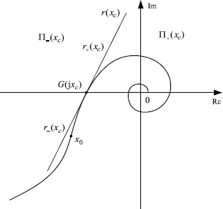
Denote the tangent line of G(jx) at the minimal crossing point xc as r(xc). Then we can prove the following proposition.
Proposition 3.29 The slope, denoted by Tc, of r(xc) is a strictly monotonically decreasing function of the parameter A, and moreover, Tc > 0 for all ![]() .
.
Proof. The slope of the tangent line r(xc) is given by
To show Tc > 0 for all ![]() it suffices to show
it suffices to show
(3.102) ![]()
By Proposition 3.27, we know that for all ![]()
So ![]() , and hence, Tc > 0 for all
, and hence, Tc > 0 for all ![]() .
.
Now we show that Tc is a strictly monotonically decreasing function of A. Note that
![]()
where G ” xA represents ![]() and all the remaining notations are the same as given in the Proof of Proposition 3.26. So from (3.101) it follows that
and all the remaining notations are the same as given in the Proof of Proposition 3.26. So from (3.101) it follows that
Straightforward computing gives
In Proof of Proposition 3.27 we have shown
So, using (3.91)–(3.94) and (3.103), we get
![]()
where the polynomial Π(xc) is defined by (3.95). Substituting (3.95) and (3.104) into the above equation yields
![]()
Therefore, Tc(A) is a strictly monotonically decreasing function of A. The proposition is thus proved. ![]()
Now, using Lemma 3.4, we can prove the following proposition.
Proposition 3.30 For all x ![]() [x0, ∞), the curve G(jx) lies on the right side of r(xc), i.e., G(jx)
[x0, ∞), the curve G(jx) lies on the right side of r(xc), i.e., G(jx) ![]() G(jxc) ∪ Π+(xc), ∀x
G(jxc) ∪ Π+(xc), ∀x ![]() [x0, ∞).
[x0, ∞).
Proof. For simplicity of statement we denote the curve of G(jx) in the parameter interval [x0, ∞) as G[x0, ∞). Also, we denote the curve G(jx) in the parameter interval (xc, ∞) as G+(xc) and the curve G(jx) in the parameter interval [x0, xc) as G−(xc). By Proposition 3.17 and Proposition 3.18, G[x0, ∞) is clockwise and has no self-intersections. Therefore, by Lemma 3.4, the only way that the curve G+(xc) can leave the half plane Π+(xc) is by crossing the line r−(xc) and the only way that G−(xc) can enter the half plane Π+(ωc) is by crossing the line r+(ωc) (see Figure 3.13). In the proof of Proposition 3.25 we have mentioned that the modulus |G(jx)| is strictly decreasing in x, and hence, |G(jx)| < |G(jxc)|, ∀x ![]() (xc, ∞). But, from Proposition 3.29, we know the slope of the tangent line at x = xc is greater than zero. This implies that the modulus of any point on r−(xc) is greater than |G(jxc)|. Therefore, it is impossible that the curve G+(xc) crosses the line r−(xc) for all x
(xc, ∞). But, from Proposition 3.29, we know the slope of the tangent line at x = xc is greater than zero. This implies that the modulus of any point on r−(xc) is greater than |G(jxc)|. Therefore, it is impossible that the curve G+(xc) crosses the line r−(xc) for all x ![]() (xc, ∞). On the other hand, from Proposition 3.28 we know that for all x
(xc, ∞). On the other hand, from Proposition 3.28 we know that for all x ![]() [x0, xc) the curve G−(xc) lies inside the third quadrant of the complex plane and hence cannot cross the line r+(xc) which is above the real axis of the complex plane. The proposition is thus proved.
[x0, xc) the curve G−(xc) lies inside the third quadrant of the complex plane and hence cannot cross the line r+(xc) which is above the real axis of the complex plane. The proposition is thus proved. ![]()
Figure 3.13 Graphic illustration of Proposition 3.30
Now, let us consider the Nyquist plots of two systems of the same form with different delay constants:
where γi is the gain margin of the transfer function
(3.106) ![]()
Lemma 3.31 If the frequency responses of systems (3.105) satisfy the following conditions:
where
(3.107) ![]()
then
![]()
holds for any given real number κ ![]() [0, 1) and any
[0, 1) and any ![]() .
.
Proof. First of all, we note that both of the two plots of the functions in the form (3.105) cross the real axis for the first time at the same point (− 1, j0) with the minimal crossing frequencies as
(3.109) ![]()
where ![]() is given by (3.98). Without loss of generality, we assume that A2 < A1. This also implies T2 < T1. Then, by Proposition 3.27, we have
is given by (3.98). Without loss of generality, we assume that A2 < A1. This also implies T2 < T1. Then, by Proposition 3.27, we have
![]()
which also implies that
![]()
since T2 < T1.
Now, we consider the lemma in the following two cases separately.
Now, we are ready to prove the following theorem.
Theorem 3.32 Suppose that the frequency responses of a family of systems are described by
(3.110) ![]()
where γi is the gain margin of the transfer function
![]()
If the following conditions hold:
where
then, ![]() does not contain the point (− 1, j0) for any given real number κ
does not contain the point (− 1, j0) for any given real number κ ![]() [0, 1) and any ω
[0, 1) and any ω ![]() [0, ∞).
[0, ∞).
Proof. Let ![]() be the minimal crossing frequency of Gi(jω). By Proposition 3.27,
be the minimal crossing frequency of Gi(jω). By Proposition 3.27, ![]() is strictly decreasing in Ai, and hence in Ti. Therefore, we have
is strictly decreasing in Ai, and hence in Ti. Therefore, we have
![]()
where ![]() is given by (3.111). Since
is given by (3.111). Since
![]()
we have
![]()
Now, we split the frequency interval [0, ∞) into two parts: ![]() and
and ![]() , and prove the theorem for the following two cases separately.
, and prove the theorem for the following two cases separately.
![]()
![]()
Therefore, summarizing the above two cases, the theorem is proved. ![]()
3.5 Frequency-Sweeping Condition
Lemma 3.1 shows that the scalability condition for symmetric multi-agent system can be verified by checking if the point (− 1, j0) is touched by the convex combination of Nyquist plots of each pair of agents. In this section we will further convert the latter into the problem of the stability test for a convex combination of two stable quasi-polynomials.
3.5.1 Stable Quasi-Polynomials
First let us recall the concept of stability of a quasi-polynomial.
A quasi-polynomial is an entire function of the form
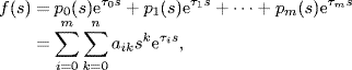
where pi(s), i = 0, 1, ![]() , m, are polynomials with coefficients
, m, are polynomials with coefficients ![]() and τ0 < τ1 <
and τ0 < τ1 < ![]() < τm are real numbers representing delays.
< τm are real numbers representing delays.
For n ≥ 0, m > 0 and any real vector τ = [τ0, τ1, ![]() , τm]T with ordered components τ0 < τ1 <
, τm]T with ordered components τ0 < τ1 < ![]() < τm, let
< τm, let ![]() denote the set of all quasi-polynomials defined by (3.114) with coefficients in
denote the set of all quasi-polynomials defined by (3.114) with coefficients in ![]() .
.
A non-constant quasi-polynomial ![]() is called Hurwitz stable or simply stable if all its roots belong to the open left half plane. The set of all Hurwitz stable quasi-polynomials in
is called Hurwitz stable or simply stable if all its roots belong to the open left half plane. The set of all Hurwitz stable quasi-polynomials in ![]() is denoted by
is denoted by ![]() .
.
Definition 3.33 A quasi-polynomial ![]() is called a global convex direction for the set
is called a global convex direction for the set ![]() if, for all stable quasi-polynomials
if, for all stable quasi-polynomials ![]() , the stability of f(s) + g(s) implies the stability of the whole segment of quasi-polynomials [f, f + g] = {f(s) + μg(s); μ
, the stability of f(s) + g(s) implies the stability of the whole segment of quasi-polynomials [f, f + g] = {f(s) + μg(s); μ ![]() [0, 1]}, i.e., if g(s) satisfies, for all
[0, 1]}, i.e., if g(s) satisfies, for all ![]() ,
,
![]()
The following lemma due to Kharitonov and Zhabko (1994) shows that the global convex direction can be verified through a frequency-sweeping test of the phase velocity.
Lemma 3.34 A quasi-polynomial ![]() is a global convex direction for the set
is a global convex direction for the set ![]() if and only if for all ω
if and only if for all ω ![]() {ω > 0 | g(jω) ≠ 0} the following condition is satisfied:
{ω > 0 | g(jω) ≠ 0} the following condition is satisfied:
(3.115) ![]()
Note that the global convex direction is defined for the set of all Hurwitz stable quasi-polynomials. To check the stability of a convex combination of two specific quasi-polynomials, we need the following definition of local convex direction.
Definition 3.35 A quasi-polynomial ![]() is called a local convex direction for a Hurwitz quasi-polynomial f(s) if the stability of f(s) + g(s) implies the stability of the whole segment of quasi-polynomials [f, f + g] = {f(s) + μg(s); μ
is called a local convex direction for a Hurwitz quasi-polynomial f(s) if the stability of f(s) + g(s) implies the stability of the whole segment of quasi-polynomials [f, f + g] = {f(s) + μg(s); μ ![]() [0, 1]}, i.e., if g(s) satisfies
[0, 1]}, i.e., if g(s) satisfies
![]()
By Definition 3.35, the following proposition is true.
Proposition 3.36 Given ![]() . Then, the following two statements are equivalent:
. Then, the following two statements are equivalent:
The following lemma gives a sufficient condition for the local convex direction.
Lemma 3.37 A quasi-polynomial ![]() is a local convex direction for the quasi-polynomial f(s) if for all ω
is a local convex direction for the quasi-polynomial f(s) if for all ω ![]() {ω > 0 : g(jω) ≠ 0} the following condition is satisfied:
{ω > 0 : g(jω) ≠ 0} the following condition is satisfied:
(3.116) ![]()
Proof. The lemma can be proved based on the fact that the phase of any Hurwitz quasi-polynomial is monotonically increasing when s goes along the imaginary axis from −j∞ to j∞. We leave the completion of the proof to the reader as an exercise. ![]()
The following lemma gives a necessary and sufficient condition of the local convex direction. It is directly from the fact that the instability of one of the polynomials ![]() , implies that there is a quasi-polynomial
, implies that there is a quasi-polynomial ![]() , with at least one zero on the imaginary axis (Gu, Kharitonov and Chen 2003).
, with at least one zero on the imaginary axis (Gu, Kharitonov and Chen 2003).
Lemma 3.38 A quasi-polynomial ![]() is a local convex direction for the quasi-polynomial f(s) if and only if the complex curve
is a local convex direction for the quasi-polynomial f(s) if and only if the complex curve
![]()
does not touch the negative real semi-axis of the complex plane.
3.5.2 Frequency-Sweeping Test
Given the normalized transfer function of time-delayed system ![]() as
as
where η, l, n are non-negative integers satisfying l ≤ n + η; Ni(s) and Di(s) are l-order and n-order real-coefficient polynomials of s, respectively; D1(s) and D2(s) are coprime. Note that Di(s) can be a constant which can be considered as a zero-order polynomial. Without loss of generality, it is assumed that 0 ≤ T1 ≤ T2. Denote
(3.118) ![]()
(3.119) ![]()
(3.120) ![]()
(3.121) ![]()
The following lemma relates the stability of a convex hull of two time-delayed systems to the robust stability of a convex combination of two Hurwitz polynomials.
Theorem 3.39 Suppose normalized transfer functions are given by (3.117), and Di(s), i = 1, 2, are coprime Hurwitz stable polynomials or positive constants. Then, the following conditions are equivalent:
Proof. “(1) ![]() (2)”. Write
(2)”. Write ![]() as
as
where λ ![]() [0, 1]. Since D1(s), D2(s) are Hurwitz stable polynomials or positive constants, by the Nyquist criterion of stability we know that the system with characteristic equation as
[0, 1]. Since D1(s), D2(s) are Hurwitz stable polynomials or positive constants, by the Nyquist criterion of stability we know that the system with characteristic equation as
is robustly stable for all λ ![]() [0, 1] if and only if
[0, 1] if and only if
![]()
From (3.122) it is easy to see that the characteristic quasi-polynomial associated with (3.123) is given by
(3.124) ![]()
Rewrite fλ(s) as
![]()
Then, the equivalence between (1) and (2) is clear.
“(2) ![]() (3)”. It follows directly from Proposition 3.36.
(3)”. It follows directly from Proposition 3.36. ![]()
Note that if we replace statement (1) in Theorem 3.39 by
then, it is not equivalent to statement (2) or (3) in Theorem 3.39. Actually, straightforward calculation will show that (3.125) is equivalent to saying
(3.126) ![]()
is Hurwitz stable. By the Nyquist criterion of stability it is equivalent to say that the system with characteristic equation as
(3.127) ![]()
is robustly stable for all λ ![]() [0, 1]. Rewrite fλ,κ(s) as
[0, 1]. Rewrite fλ,κ(s) as
![]()
Note that the Nyquist plots of normalized transfer-functions ![]() , i = 1, 2, cross the real axis at the point (− 1, j0). Therefore,
, i = 1, 2, cross the real axis at the point (− 1, j0). Therefore, ![]() , i = 1, 2, do not contain the point (− 1, j0) for any ω
, i = 1, 2, do not contain the point (− 1, j0) for any ω ![]() [0, ∞) and any κ
[0, ∞) and any κ ![]() [0, 1). Since Di(s), i = 1, 2, are Hurwitz stable polynomials or positive constants, by the Nyquist criterion of stability again, we know the systems with the following characteristic equations
[0, 1). Since Di(s), i = 1, 2, are Hurwitz stable polynomials or positive constants, by the Nyquist criterion of stability again, we know the systems with the following characteristic equations
![]()
are stable. This implies that quasi-polynomials
![]()
are Hurwitz stable. Therefore, by Definition 3.33 we know that fλ,κ(s) is Hurwitz stable if and only if the quasi-polynomial
![]()
is a local convex direction for f0,κ(s), or simply if it is a convex direction. The following lemma summarizes the above discussion.
Theorem 3.40 Suppose normalized transfer functions are given by (3.117), and Di(s), i = 1, 2, are coprime Hurwitz stable polynomials or positive constants. Then,
![]()
if and only if g(s) = N2(s)D1(s)e−T2s − N1(s)D2(s)e−T1s is a local convex direction for f0,κ(s), or simply if g(s) is convex direction.
Now, we can generalize the result of Theorem 3.40 to a family of n normalized systems.
Theorem 3.41 Consider a family of normalized systems described by
(3.128) ![]()
Suppose that
(3.129) ![]()
Then,
![]()
if for any ![]() , the quasi-polynomial
, the quasi-polynomial
![]()
is a convex direction.
Proof. Suppose Nk(s)Di(s)e−Tks − Ni(s)Dk(s)e−Tis is a convex direction. Then, by Theorem 3.40, we know that
holds for any ![]() . Note that
. Note that
also holds for any ![]() since
since ![]() does not contain (− 1, j0) and the origin is inside the region enclosed by
does not contain (− 1, j0) and the origin is inside the region enclosed by ![]() . Also, note that
. Also, note that
![]()
holds when ω→ ∞ since ![]() . Therefore, by continuity of the set
. Therefore, by continuity of the set ![]() on ω, if
on ω, if ![]() intersects the point (− 1, j0) then its boundary,
intersects the point (− 1, j0) then its boundary, ![]() or
or ![]() will definitely intersects the point (− 1, j0) for some ω*
will definitely intersects the point (− 1, j0) for some ω* ![]() [0, ∞). But (3.130) and (3.131) have excluded the possibility. Therefore, we conclude that
[0, ∞). But (3.130) and (3.131) have excluded the possibility. Therefore, we conclude that
![]()
Theorem is thus proved. ![]()
3.6 Notes and References
The concept and expression of the signed curvature for parametric equation a curve can be found in many textbooks on classical differential geometry such as Guggenheimer (1977).
The clockwise property of the Nyquist plot of transfer functions attracted attention of control researchers as early as the 1980s (Horowitz and Ben-Adam (1989). It was found useful in the study of absolute stability (Tesi et al. 1992). Lemma 3.5 was initially given in Tesi et al. 1992) and extended to the current version in Tian and Yang (2004a).
In 1990s, convexity, a notion very closely related to the clockwise property, was proved for the frequency response arc of stable polynomials as a by-product of the study of robust stability against parametric uncertainties (Gu 1994; Hamann and Barmish 1993). Rantzer (1992) studied the relationship between the phase velocity of the frequency response plot of polynomials and the robust stability of a convex set of stable polynomials, and proposed the notion of convex direction in the space of stable polynomials. Kharitonov and Zhabko (1994) extended the notion of convex direction to the space of stable quasi-polynomials.
The relationship between the scalability of a distributed congestion control algorithm and differential geometric properties of the frequency response of the control system was uncovered in Tian and Yang (2004a). In this chapter it was shown that the clockwise property of the frequency response curve (Nyquist plot) of a congestion control system plays a key role in the scalability of the stability criterion for a network with diverse round-trip delays. Besides, some other differential geometric properties, such as phase monotonicity and/or modulus monotonicity, critical point of clockwise property, phase velocity, etc., are also shown to be very important in the scalability analysis for distributed congestion control systems (Tian 2005a,b; Tian and Chen 2006). In Tian and Liu (2008) and Tian and Liu (2009) it was revealed that the scalability of consensus criteria for multi-agent systems with diverse input delays are also closely related to differential geometric properties of node dynamics of networks.
The material of Section 3.3 is taken from Tian and Yang (2004a,b). Section 3.4 is based on Tian (2005a); Tian and Chen (2006) while Section 3.5 is based on Kharitonov and Zhabko (1994) and Tian (2005b).
Gu K (1994). Comments on “Convexity of frequency response arcs associated with a stable polynomials”. IEEE Transactions on Robotics and Automation, 39, 2262–2265.
Gu K, Kharitonov VL and Chen J (2003). Stability of Time-delayed Systems. Birkhäuser, Boston.
Guggenheimer HW (1977). Differential Geometry. Dover, New York.
Hamann JC and Barmish BR (1993). Convexity of frequency response arcs associated with a stable polynomial. IEEE Transactions on Bobotics and Automation, 38, 904–915.
Horowitz I and Ben-Adam S (1989). Clockwise nature of Nyquist locus of stable transfer functions. International Journal Control, 49, 1433–1436.
Kharitonov VL and Zhabko AP (1994). Robust stability of time-delayed systems. IEEE Transactions on Automatic Control, 39, 2388–2397.
Rantzer A (1992). Stability conditions for polytopes of polynomials. IEEE Transactions on Automatic Control, 37, 79–84.
Tesi A, Vicino A and Zappa G (1992). Clockwise property of the Nyquist plot with implications for absolute stability. Automatica, 28, 71–80.
Tian Y-P and Yang H-Y (2004a). Stability of the Internet congestion control with diverse delays. Automatica, 40, 1533–1541.
Tian Y-P and Yang H-Y (2004b). Stability of distributed congestion control with diverse communication delays. Proceedings of the World Congress on Intelligent Control and Automation 2, 1438–1442.
Tian Y-P (2005a). Stability analysis and design of the second-order congestion control for networks with heterogeneous delays. IEEE/ACM Transactions on Networking, 13, 1082–1093.
Tian Y-P (2005b). A general stability criterion for congestion control with diverse communication delays. Automatica, 41, 1255–1262.
Tian Y-P and Chen G (2006). Stability of the primal-dual algorithm for congestion control. International Journal of Control, 79, 662–676.
Tian Y-P and Liu C-L (2008). Consensus of multi-agent systems with diverse input and communication delays. IEEE Transactions on Automatic Control, 53, 2122–2128.
Tian Y-P and Liu C-L (2009). Robust consensus of multi-agent systems with diverse input delays and asymmetric interconnection perturbations. Automatica, 45, 1347–1353.