
Chapter 4
Congestion Control: Model and Algorithms
To which sources are the sun and the moon linked? In what formation are the stars deployed?
–Qu Yuan (340–278 BC), ‘Heavenly Questions'
Congestion avoidance mechanisms serve as a keystone of a huge communication network like the Internet. This chapter introduces basic notions, algorithms and system models of end-to-end congestion control. The congestion control problem is modeled as an optimization problem of resource allocation in the network under link capacity constraints, and the congestion control algorithms are treated as distributed real-time gradient-descent algorithms of seeking for the optimal solution of the resource allocation problem.
4.1 An Introduction to Congestion Control
Consider a network containing S sources each of which is identified as an origin. Denote by ![]() the set of source nodes. It is supposed that each user uses a fixed route between its origin and destination. Denote by
the set of source nodes. It is supposed that each user uses a fixed route between its origin and destination. Denote by ![]() the set of all the links contained in the network, and by
the set of all the links contained in the network, and by ![]() the set of links used by the user of source i. Note that each link may be used by multiple sources. Denote by
the set of links used by the user of source i. Note that each link may be used by multiple sources. Denote by ![]() the set of sources using link l. From the viewpoint of graph theory, the interconnection topology of such a network is a bipartite graph with vertex classes
the set of sources using link l. From the viewpoint of graph theory, the interconnection topology of such a network is a bipartite graph with vertex classes ![]() and
and ![]() . Li is the neighbor set of source node i, and Sl is the neighbor set of link node l.
. Li is the neighbor set of source node i, and Sl is the neighbor set of link node l.
Each source ![]() transmits data at rate xi (bits/sec or bps) from the origin to its destination. Each link l in the network has a capacity cl bps, which implies that the sum of the transmission rates of all the users sharing link l is less than or equal to cl, i.e.,
transmits data at rate xi (bits/sec or bps) from the origin to its destination. Each link l in the network has a capacity cl bps, which implies that the sum of the transmission rates of all the users sharing link l is less than or equal to cl, i.e.,
4.1.1 Congestion Collapse
Since the capacity of all the links is limited, the network may suffer congestion collapse. Now, we explain the reason of congestion collapse with an example. Firstly, we assume that if the offered traffic on link l exceeds the capacity cl of the link, then all sources sharing link l see their traffic reduced in proportion to their offered traffic. This assumption is approximately true if the queueing is first-in first-out (FIFO) in the network node.
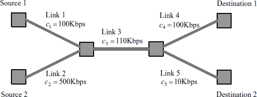
Consider a simple network with two sources as shown in Figure 4.1. There are five links labeled 1 through 5 with capacities shown on the figure. Assume that sources are limited only by their first link, without feedback from the network. Then, source 1 and source 2 may send packets at rate 100 Kbps and 500 Kbps, respectively, according to their first links. But, source 1 can actually only send at 10 Kbps because it is competing with source 2 on link 3, which sends at a higher rate on that link; however, source 2 is limited to 10 Kbps because of link 5. Therefore, the outgoing rates of source 1 and source 2 are both 10 Kbps, and the total throughput is only 20 Kbps! If source would be aware of the global situation, and if it were to cooperate, then it would send at 10 Kbps only initially, which would allow source 1 to send at 100 Kbps, without any penalty for source 2. Then, the total throughput of the network would become 110 Kbps.
Figure 4.1 A simple network exhibiting inefficiency.
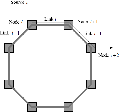
The above example show some inefficiency in network communication. In complex network scenarios, such inefficiency may lead to a form of instability known as congestion collapse. Let us illustrate this by using the network shown in Figure 4.2. This network topology is a ring which is commonly used in network design. Suppose there are n nodes and links numbered 1, ![]() , n. Source i enters node i using links i and [i mod n] + 1, and leaves at node [(i + 1) mod n] + 1. Assume that source i sends as much as xi, without feedback from the network. Denote by x ' i the achieved rate of source i through link i at node [i mod n] + 1, and by x ” i the achieved rate of source i through link [i mod n] + 1 at node [(i + 1) mod n] + 1. In the rest of the example we omit “mod n” when the context is clear. Then, we have
, n. Source i enters node i using links i and [i mod n] + 1, and leaves at node [(i + 1) mod n] + 1. Assume that source i sends as much as xi, without feedback from the network. Denote by x ' i the achieved rate of source i through link i at node [i mod n] + 1, and by x ” i the achieved rate of source i through link [i mod n] + 1 at node [(i + 1) mod n] + 1. In the rest of the example we omit “mod n” when the context is clear. Then, we have
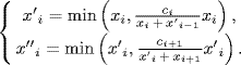
For simplicity we assume that ci = c and xi = x for ![]() . Then, we have obviously x ' i = x ' and x” i = x ” for some values of x ' and x” which are computed below. If x ≤ c/2 then there is no loss and x ' = x ” = x and the throughput of the network is nx. Otherwise, from (4.2) it follows that
. Then, we have obviously x ' i = x ' and x” i = x ” for some values of x ' and x” which are computed below. If x ≤ c/2 then there is no loss and x ' = x ” = x and the throughput of the network is nx. Otherwise, from (4.2) it follows that
![]()
which yields
From (4.2) it also follows that
Combining (4.3) and (4.4) gives
By using the Taylor expansion, from (4.5) it is easy to get
(4.6) ![]()
where ![]() denotes the terms with order equal to or greater than two. When the offered rate x goes to ∞, the outgoing rate approaches zero, and the throughput of the network nx” also approaches zero. This is the so-called congestion collapse. Therefore, to avoid congestion collapse, each source should limit its sending rate by taking into consideration the state of the network.
denotes the terms with order equal to or greater than two. When the offered rate x goes to ∞, the outgoing rate approaches zero, and the throughput of the network nx” also approaches zero. This is the so-called congestion collapse. Therefore, to avoid congestion collapse, each source should limit its sending rate by taking into consideration the state of the network.
Figure 4.2 A ring network illustrating congestion collapse.
4.1.2 Efficiency and Fairness
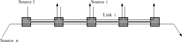
How to allocate the resources of networks? We have shown that the efficiency is a very important issue to be considered. However, we will show that there is another important factor in this design. Let us consider an example network shown by Figure 4.3, where n sources share n − 1 links. All links have a capacity equal to c. We assume that some congestion avoidance strategy has been implemented in the network and there is negligible packet loss. Source i sends data at rate ![]() . To achieve the maximum efficiency, the following equality should hold
. To achieve the maximum efficiency, the following equality should hold
![]()
So, the total throughput of the network is
![]()
Obviously, if we want to maximize the total throughput of the network, we should set xn = 0. This strategy is, of course, unfair to source n. In summary, the objective of congestion control is to provide both efficiency and some form of fairness.
Figure 4.3 A network illustrating efficiency and fairness.
4.1.3 Optimization-Based Resource Allocation
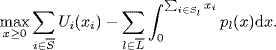
To optimize the resource allocation in the network, we suppose that each user ![]() generates a utilityUi(xi) when a data rate xi is allocated to it. Then, the network resource can be allocated by solving the following optimization problem
generates a utilityUi(xi) when a data rate xi is allocated to it. Then, the network resource can be allocated by solving the following optimization problem
subject to (4.1). From optimization theory (Bertsekas (1995), the above optimization problem has a unique solution if ![]() , are strictly concave functions. It is also reasonable to assume that
, are strictly concave functions. It is also reasonable to assume that ![]() , are non-decreasing because more resources generate higher utility. Therefore, we make the following assumption for the utility function.
, are non-decreasing because more resources generate higher utility. Therefore, we make the following assumption for the utility function.
Assumption 4.1 For each ![]() , Ui(xi) is a continuously differentiable, non-decreasing, strictly concave function.
, Ui(xi) is a continuously differentiable, non-decreasing, strictly concave function.
Denote by ![]() the optimal solution to the resource allocation problem (4.7). From a well-known property of convex functions it follows that
the optimal solution to the resource allocation problem (4.7). From a well-known property of convex functions it follows that
where ![]() is the derivative of Ui(xi) at
is the derivative of Ui(xi) at ![]() ,
, ![]() is any other set of transmission rates satisfying the constraints (4.1). Rewrite (4.8) as
is any other set of transmission rates satisfying the constraints (4.1). Rewrite (4.8) as
As ![]() is the relative change of the source i's rate,
is the relative change of the source i's rate, ![]() can be regarded as a fairness weight for source i. Then, (4.9) implies that the weighted sum of the changes in each user's rate is less than or equal to zero. Next, we show that different choices of the utility function lead to different kind of fairness.
can be regarded as a fairness weight for source i. Then, (4.9) implies that the weighted sum of the changes in each user's rate is less than or equal to zero. Next, we show that different choices of the utility function lead to different kind of fairness.
Proportional fairness
Let us choose, for example,
where ![]() . Then, the inequality (4.8) becomes
. Then, the inequality (4.8) becomes
(4.11) ![]()
The above inequality implies that the weighted sum of the proportional changes in each user's rate is less than or equal to zero. Hence, the resource allocation corresponding to the choice of the utility function ![]() is said to be weighted proportionally fair. In particular, if all
is said to be weighted proportionally fair. In particular, if all ![]() 's are equal to one, then the allocation is simply said to be proportionally fair.
's are equal to one, then the allocation is simply said to be proportionally fair.
Minimum potential delay fairness
Let us choose, for example,
(4.12) ![]()
where ![]() . Then, the inequality (4.8) becomes
. Then, the inequality (4.8) becomes
(4.13) ![]()
Suppose that ![]() represents the size of the file that source i is attempting to transmit, then
represents the size of the file that source i is attempting to transmit, then ![]() is the amount of time that it would take to transfer the file, and
is the amount of time that it would take to transfer the file, and ![]() is the minimum of the sum of the amount of time. Hence, the resulting resource allocation under this choice of utility function is said to be minimum potential delay fair.
is the minimum of the sum of the amount of time. Hence, the resulting resource allocation under this choice of utility function is said to be minimum potential delay fair.
4.2 Distributed Congestion Control Algorithms
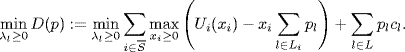
To solve the optimization problem (4.7), one has to know the utility functions and routes of all the sources in the network. In a huge network such as the Internet, this information is not available centrally. Thus, it is important to develop distributed solutions, where each source adapts its transmission rate based only on local information.
4.2.1 Penalty Function Approach and Primal Algorithm
Instead of trying to obtain the optimal solution to problem (4.7), let us consider the following problem where the constraints are added to the objective using penalty function:
The function pl(x) denotes the penalty function corresponding to the capacity cl of link l. It is also referred to as the price at link l. Note that the price at link l is a function of the aggregate arrival source rate ![]() at link l, and can be regarded as a measure of congestion at link l. We make the following assumption on the price function.
at link l, and can be regarded as a measure of congestion at link l. We make the following assumption on the price function.
Assumption 4.2 For each ![]() , pl(·) is a non-decreasing, continuous function such that
, pl(·) is a non-decreasing, continuous function such that
![]()
The first-order necessary condition of the optimization problem (4.14) is given by
![]()
Thus, the optimization problem (4.14) can be solved by using the following continuous-time version of gradient-ascent algorithm:
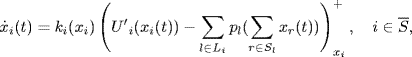
where the step size ki(x) is any non decreasing, continuous function such that ki(x) > 0; ![]() is defined as
is defined as
![]()
which ensures the non-negativeness of variable x.
Obviously, (4.15) is a distributed control algorithm as each source node uses only the price information of the links used by this source, and each link needs only the rate information of the sources sharing this link.
Since the optimization problem (4.14) has unique optimal solution under Assumption 4.1., the equilibrium point of the congestion control equation (4.15) solves (4.14). As shown by Srikant (2004), the objective in (4.14) is a Lyapunov function for the system of equations given by (4.15), and the derivative of the Lyapunov function is negatively definite if the price functions satisfy Assumption 4.2. Hence, the system given by (4.15) is globally asymptotically stable with respect to the optimal solution of (4.14).
In the literature on congestion control, the algorithm (4.15) is referred to as the primal algorithm. If we apply the utility function given by (4.10) for the proportional fairness and take a linear step size function, i.e.,
![]()
where κi > 0, then, the primal algorithm (4.15) becomes
(4.16) 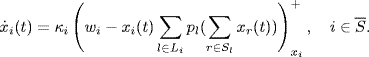
Kelly, Maulloo and Tan (1998) first proposed this primal algorithm and proved the global convergence of the algorithm. So, this algorithm is also referred to as Kelly's primal algorithm.
4.2.2 Dual Approach and Dual Algorithm
Instead of solving the optimization problem (4.7) using a penalty function, one can also solve the problem exactly using Lagrange multipliers. Low and Lapsley (1999) considered the associated dual problem:
Given the Lagrange multipliers pl's which are also referred to as prices, the maximization over xi can be carried out by each source based on the aggregate price of its route as follows:
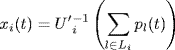
where ![]() denotes the inverse of the derivative of Ui. Note that
denotes the inverse of the derivative of Ui. Note that ![]() is a decreasing function when Ui(·) is convex.
is a decreasing function when Ui(·) is convex.
The continuous-time version of the gradient projection algorithm for the dual problem (4.17) is given by
![]()
where γl > 0 is a step size parameter (also referred to as a control gain) at link l. It is easy to get that
![]()
Thus, one can get an algorithm to compute the price at each link as follows:
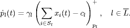
The algorithm (4.19) together with (4.18) is called a dual algorithm in the literature on congestion control. The interpretation of the algorithm is very clear: if the demand ![]() exceeds capacity cl, increase the price; otherwise, decrease it. The algorithm is distributive because each link uses only the total arrival rate into it to compute its price.
exceeds capacity cl, increase the price; otherwise, decrease it. The algorithm is distributive because each link uses only the total arrival rate into it to compute its price.
4.2.3 Primal-Dual Algorithm
The dual solution (or the corresponding dual algorithm) solves the resource allocation problem (4.7) exactly, whereas the penalty function approach (or the corresponding primal algorithm) solves it only approximately. From (4.19) it is clear that at the equilibrium it holds
![]()
This implies that the dual algorithm can achieve very high utilization of link capacity. However, the dual algorithm requires the existence of the inverse of the derivative of the utility function. So, it is restricted to a specific class of utility functions, and hence, does not allow arbitrary fairness in rate allocation. To achieve both high utilization and arbitrary fairness, a so-called primal-dual algorithm was proposed in Alpcan and Ba![]() ar (2003), Wen and Arcak (2003) and generalized in Liu et al.(2003). The main idea of the primal-dual algorithm is to adopt dynamical adaptations both at links and at sources, which can be described as follows:
ar (2003), Wen and Arcak (2003) and generalized in Liu et al.(2003). The main idea of the primal-dual algorithm is to adopt dynamical adaptations both at links and at sources, which can be described as follows:
(4.20) 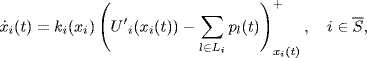
(4.21) 
4.2.4 REM: A Second-Order Dual Algorithm
Generally, the congestion control algorithms for Internet-like networks can be classified into two types: one is the algorithms implemented in its transmission control protocol (TCP), such as TCP Reno and TCP Vegas, which adjust transmission rates of sources based on available feedback congestion marks (Jacobson (1988). The other is the algorithms, such as DropTail and RED, used as the active queue management (AQM) at the link nodes, which decide how to drop arriving packets when the network is overloaded (Floyd and Jacobson (1993). As we have shown in this chapter, the primal algorithm has a dynamical law for adjusting source rate and a static law for generating link price, and such an algorithm properly describes currently used congestion avoidance protocols for TCP rate control at sources. Similarly, the dual algorithm has a dynamical law for adjusting link price and a static law for generating source rate, and such an algorithm can be used for the AQM mechanism at links.
When the dual algorithm is used for AQM, the price pl, the measure of congestion at link l, is usually given some practical meaning. For example, the queue length in the buffer is used as the congestion measure in RED (Floyd and Jacobson (1993). However, when the dual algorithm (4.19) is used for adjusting the queue length, we find that at the equilibrium the queue length may be far away from the target value. To keep the queue length around a desired value, Athuraliya, Low and Yin (2001) proposed a kind of the second-order AQM control algorithm: random exponential marking (REM). The continuous-time version of the REM algorithm is given by
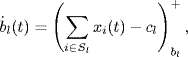
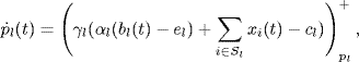
where ![]() , are the control gains. Obviously, REM reduces to the (first-order) dual algorithm if αl = 0.
, are the control gains. Obviously, REM reduces to the (first-order) dual algorithm if αl = 0.
If the queue length is taken as the congestion measure, then bl(t) can be understood as the queue length at link l and el is the desired value of the queue length. Under the algorithm given by (4.22) and (4.23), the equilibrium point guarantees not only the tight utilization of the link capacity, i.e., ![]() , but also the desired value the queue length, i.e., bl = el.
, but also the desired value the queue length, i.e., bl = el.
4.3 A General Model of Congestion Control Systems
4.3.1 Framework of End-to-End Congestion Control under Diverse Round-Trip Delays
Recall that the network under our consideration has S sources which share L links. We have supposed that there is only one fixed route between each user's origin and its destination, and the set of links contained in source i's route is denoted by Li. By the sets Li's we can define an L × S routing matrix R = {Rli}, where
(4.24) ![]()
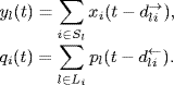
For each link l, we have the following:
- aggregate rate of all sources which use link l, denoted by yl (bps);
- price pl, used to indicate the link congestion.
The vectors ![]() are defined by the above components across the set of links.
are defined by the above components across the set of links.
For each source i, we have the following:
- source rate xi (bps);
- aggregate price of all links used by source i, denoted by qi.
The vectors ![]() are defined by the above components across the set of sources.
are defined by the above components across the set of sources.
The following equations reflect the interconnection between links and sources:
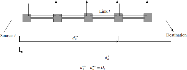
For a given link l and each source i ![]() Sl, let
Sl, let ![]() denote the forward delay of delivering packets from source i to link l, and
denote the forward delay of delivering packets from source i to link l, and ![]() the backward delay of sending the feedback signal from link l to source i. Then, each route is subject to a round-trip delay denoted by Di. We assume that for any
the backward delay of sending the feedback signal from link l to source i. Then, each route is subject to a round-trip delay denoted by Di. We assume that for any ![]() the following relationship is true (Johari and Tan (2001)
the following relationship is true (Johari and Tan (2001)
The assumption (4.27) is quite reasonable for currently used TCP. It implies that the forward delay from source i to any link l in its route plus the backward delay from the link is the same for any l. An illustration of the round-trip delay is given by Figure 4.4.
Figure 4.4 An illustration of round-trip delay.
When propagation delays are considered, the following relationships are immediate from (4.25) and (4.26):
Now, we can summarize the end-to-end congestion control algorithms previously introduced under diverse round-trip delays as follows.
Primal algorithm
At source ![]() :
:
(4.29) ![]()
At link ![]() :
:
(4.30) ![]()
Dual algorithm
At source i:
(4.33) ![]()
At link l:
(4.34) ![]()
Primal dual algorithm
At source i:
(4.36) ![]()
(4.37) ![]()
At link l:
(4.38) ![]()
(4.39) ![]()
Second-order dual algorithm
At source i:
(4.40) ![]()
(4.41) ![]()
At link l:
(4.42) ![]()
(4.43) ![]()
(4.44) ![]()
4.3.2 General Primal-Dual Algorithm
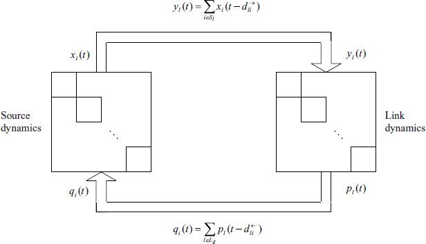
Let ![]() be some internal variable at source i, which is subject to a dynamical adjustment. The source rate xi(t) is adjusted according to a function Fi based on αi(t) and qi(t). So the source dynamics are described as follows:
be some internal variable at source i, which is subject to a dynamical adjustment. The source rate xi(t) is adjusted according to a function Fi based on αi(t) and qi(t). So the source dynamics are described as follows:
(4.46) ![]()
Similarly, let ![]() be some internal variable at link l, which is subject to a dynamical adjustment. The link congestion measure pl(t) is adjusted according to a function El based on βl(t) and yl(t). So the link dynamics are described as follows:
be some internal variable at link l, which is subject to a dynamical adjustment. The link congestion measure pl(t) is adjusted according to a function El based on βl(t) and yl(t). So the link dynamics are described as follows:
(4.47) ![]()
Sources and links are interconnected by the following equations:
(4.49) ![]()
Equations (4.45)–(4.50) constitute a dynamical feedback system with structure shown by Figure 4.5. For the statement convenience, we call the system “system ∑” in the rest of this chapter.
Figure 4.5 Feedback structure of distributed congestion control.
Remark 1. The model (4.45)–(4.48) unifies different congestion control algorithms. For example, one can set xi(t) = Fi(αi(t), qi(t)) = αi(t) in the source dynamics, and Vl(·, ·) ≡ 0, βl(t) ≡ 0 in the link dynamics, then get the primal algorithm. Table 4.1 summarizes the relationship of the unified model with other algorithms.
Table 4.1 Different congestion control algorithms in a unified model.
| first-order | second-order | |
| Primal algorithm | βl(t) ≡ 0, | βl(t) ≡ 0, |
| Vl(·, ·) ≡ 0, | Vl(·, ·) ≡ 0. | |
| Fi(αi(t), qi(t)) = αi(t). | ||
| Dual algorithm | αi(t) ≡ 0, | αi(t) ≡ 0, |
| Hi(·, ·) ≡ 0, | Hi(·, ·) ≡ 0. | |
| El(βl(t), yl(t)) = βl(t). | ||
| Primal-dual algorithm | Fi(αi(t), qi(t)) = αi(t), | |
| El(βl(t), yl(t)) = βl(t). |
Remark 2. For the second-order case, the only algorithm considered in this book is the REM algorithm. In the unified model, by setting βl(t) = [bl(t), pl(t)]T, where bl(t) is a scalar internal variable at link l, and El(·, ·) = [0, I]βl(t), then we get the REM algorithm.
4.3.3 Frequency-Domain Symmetry of Congestion Control Systems
In this section we derive the linearized model of the congestion control system ∑ and show its symmetry property in the frequency domain.
Let θ = (αT, xT, βT, pT)T. Assume that system ∑ has an isolated equilibrium point
![]()
Let ![]() ,
, ![]() ,
, ![]() ,
, ![]() , and
, and
Linearized equations of the dynamics at source i are
(4.53) ![]()
(4.54) ![]()
where ![]() ,
, ![]() ,
, ![]() , and
, and ![]() . In the Laplace domain, the above equations can be written as
. In the Laplace domain, the above equations can be written as
where Xi(s) and Qi(s) are the Laplace transformation of ![]() and
and ![]() , respectively. Denote
, respectively. Denote
(4.56) ![]()
Let κi be the control gain at source i, which is defined as
(4.57) ![]()
where ν is the order of the pole s = 0 contained in ![]() . Define
. Define
(4.58) ![]()
Then, we have
(4.59) ![]()
Similarly, linearized equations of the dynamics at link l are
(4.60) ![]()
(4.61) ![]()
where ![]()
![]()
![]() , and
, and ![]() . The equivalent equation in the Laplace domain is
. The equivalent equation in the Laplace domain is
where Pl(s) and Yl(s) are the Laplace transformation of ![]() and
and ![]() , respectively. Denote
, respectively. Denote
(4.63) ![]()
Let γl be the control gain at link l, which is defined as
(4.64) ![]()
where μ is the order of the pole s = 0 contained in ![]() . Define
. Define
(4.65) ![]()
Then we have
(4.66) ![]()
Assume that the system is semi-homogeneous by links, which implies that all the links used by the same source have the same dynamics with possibly different gains, i.e.,
![]()
Then, we can write
(4.67) ![]()
Denote
(4.68) ![]()
We refer to Wi(s) as the round-trip transfer function of the route associated with source i.
In the Laplace domain, equations (4.51) and (4.52) can be written as
Define the delayed forward routing matrix Rf(s) and the backward routing matrix Rb(s) as
(4.71) 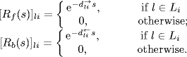
Then, from the assumption on the round-trip delay (4.27) it follows that
Combining (4.55), (4.62), (4.69) and (4.70) we get
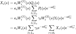
Denote
(4.74) ![]()
(4.75) ![]()
(4.76) ![]()
(4.77) ![]()
Then, by using relationship (4.72), equation (4.73) can be rewritten in the following matrix form:
(4.78) ![]()
Then, we get the open-loop transfer function of system ∑ as
Now, we see that system ∑ is symmetric in the frequency domain by Definition 2.2.
4.4 Notes and References
In 1988, Jacobson (1988) proposed a remarkable congestion avoidance algorithm, which is now regarded as a significant technological breakthrough for the growth of the Internet from a small-scale research network to today's interconnection of tens of millions of users and links. The optimization problem (4.7) was first formulated in Kelly (1997). The dual optimization problem (4.17) was first considered in Low and Lapsley (1999). Related ideas also appeared in Yaiche, Mazumdar and Rosenberg (2000). Kar, Sarkar and Tassiulas (2001) extended these ideas to multicast networks.
The mathematical treatment of congestion control problems and algorithms in this chapter follows the classic literature on congestion control theory, see, for example, Srikant (2004), Kelly (2003), Low, Paganini and Doyle (2002). The formulation of the general model of congestion control algorithms given in Section 4.3.2 and its linearization with symmetry analysis given in Section 4.3.3 are mainly taken from Tian (2005). For the connection of the algorithms with currently used Internet protocols such as TCP Reno and TCP Vegas (Brakmo and Peterson 1995; Jacobson 1988), DropTail and RED (Floyd and Jacobson 1993), etc., the reader is referred to Low, Paganini and Doyle (2002).
Bertsekas D (1995). Nonlinear Programming. Athena Scientific, Belmont, MA.
Srikant R (2004). The Mathematics of Internet Congestion Control. Birkhäuser, Boston.
Alpcan T and Ba![]() ar T (2003). A utility-based congestion control scheme for internet-style networks with delay. Proceedings of IEEE Infocom, San Francisco, California.
ar T (2003). A utility-based congestion control scheme for internet-style networks with delay. Proceedings of IEEE Infocom, San Francisco, California.
Athuraliya S, Low SH and Yin Q (2001). REM: Active Queue Management. IEEE Network, 15, 48–53.
Brakmo LS and Peterson LL (1995). TCP Vegas: end to end congestion avoidance on a global Internet. IEEE Journal on Selected Area in Communications 13, 1465–1480.
Floyd S and Jacobson V (1993). Random early detection gateways for congestion avoidance. IEEE/ACM Transactions on Networking, 1, 397–413.
Jacobson V (1988). Congestion avoidance and control. Proceedings of ACM SIGCOMM ’88, Stanford, CA, 314–329.
Johari R and Tan D (2001). End to end congesion control for the internet: delays and stability. IEEE/ACM Transactions on Networking, 9, 818–832.
Kar K, Sarkar S and Tassiulas L (2001). Optimization based rate control for multirate multicast sessions. Proceedings of IEEE Infocom.
Kelly FP (1997). Charging and rate control for elastic traffic. European transactions on Telecommunication, 8, 33–37.
Kelly FP, Maulloo A and Tan D (1998). Rate control for communication networks: shadow prices proportional fairness and stability. Journal of the Operational Research Society, 49, 237–252.
Kelly FP (2003). Fairness and stability of end-to-end congestion control. European Journal of Control, 9, 149–165.
Liu S, Ba![]() ar T and Srikant R (2003). Controlling the Internet: A survey and some new results. Proceedings of IEEE Conference on Decision and Control, Maui, Hawaii.
ar T and Srikant R (2003). Controlling the Internet: A survey and some new results. Proceedings of IEEE Conference on Decision and Control, Maui, Hawaii.
Low SH and Lapsley DE (1999). Optimization flow control, I: basic algorithm and convergence. IEEE/ACM Transactions on Networking, 7, 861–874.
Low SH, Paganini F and Doyle JC (2002). Internet congestion control. IEEE Control Systems Magazine, 22, 28–43.
Tian Y-P (2005). A general stability criterion for congestion control with diverse communication delays. Automatica, 41, 1255–1262.
Wen JT and Arcak M (2003). A unifying passivity framework for network flow control. Proceedings of IEEE Infocom, San Francisco, California.
Yaiche H, Mazumdar RR and Rosenberg C (2000). A game theoretical framework for bandwidth allocation and pricing in broadband networks. IEEE/ACM Transactions on Networking, 8, 2–14.