
Chapter 5
Congestion Control: Stability and Scalability
The net of Heaven has large meshes but yet it lets nothing through.
—Lao Dan (580–500 BC), Tao Te Ching
A distributed congestion control system with diverse propagation delays enjoys symmetry property in the frequency domain. This chapter applies the stability and scalability results presented in Chapter 2 and Chapter 3 to derive scalable stability criteria for the congestion control algorithms introduced in Chapter 4. The mechanism of time-delayed feedback control in the stabilization of distributed congestion control systems is also investigated.
5.1 Stability of the Primal Algorithm
5.1.1 Johari–Tan Conjecture
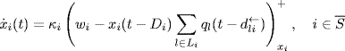
With the choice of utility function ![]() , and the step size function ki(xi) = κixi, the primal algorithm (4.15) has the form (Kelly, Maulloo and Tan (1998)
, and the step size function ki(xi) = κixi, the primal algorithm (4.15) has the form (Kelly, Maulloo and Tan (1998)
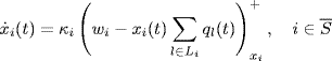
where ![]() is the transmission rate at source i, κi > 0 is the control gain,
is the transmission rate at source i, κi > 0 is the control gain, ![]() is some desired value of the rate of marked packets received back at source i, and the notation
is some desired value of the rate of marked packets received back at source i, and the notation ![]() means
means
![]()
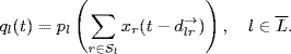
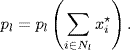
The first equation (5.1) describes the time evolution of the transmission rate xi(t) of source i. The second equation (5.2) describes the generation of congestion signal ql(t) at link l, by means of a congestion indication function pl(y), which is assumed to be increasing, nonnegative, and not identically zero. A candidate of p(y) is p(y) = 1 − ey(1 − y), which is positive and strictly increasing for all y > 0 (Johari and Tan (2001).
It was shown by (Kelly, Maulloo and Tan (1998) the system of equations (5.1) and (5.2) has a unique equilibrium point ![]() given by
given by
and this equilibrium is globally asymptotically stable. Johari and Tan (2001) studied the influence of propagation delays on the stability of congestion control algorithms by considering the following delay difference equations analogous to the equations (5.1) and (5.2):
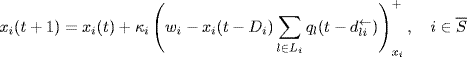
where the forward delay ![]() and the backward delay
and the backward delay ![]() are subject to (4.27). Note that the equilibrium of system (5.4)–(5.5) has the same expression as given by (5.3).
are subject to (4.27). Note that the equilibrium of system (5.4)–(5.5) has the same expression as given by (5.3).
Johari and Tan (2001) proposed the following conjecture on the local stability of the equilibrium point of system (5.4)–(5.5).
Conjecture 5.1 Let![]() , be diverse round-trip delays. System (5.4)–(5.5) is locally stable at the equilibrium point x*, if
, be diverse round-trip delays. System (5.4)–(5.5) is locally stable at the equilibrium point x*, if
(5.6) 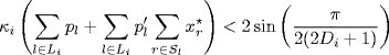
holds for all ![]() , where
, where
(5.7) 
and pl′ is the derivative of pl evaluated at ![]() , i.e.,
, i.e.,
(5.8) 
The significance of this conjecture can be explained as follows. If it is correct, then the network stability under diverse round-trip delays can be guaranteed by implementation of a simple distributed congestion control algorithm called the primal algorithm, and the stability test for such a network uses only local information of each user of the network. Hence, such a control scheme fully satisfies the scalability requirement for huge networks such as the Internet. Moreover, the conjecture looks so elegant because it gives a necessary and sufficient condition of stability for system (5.4)–(5.5) when only one source is contained in the network.
Johari and Tan (2001) proved the correctness of the conjecture for a special case when all sources share the same round-trip delay parameter, i.e., Di = D for all ![]() . They also generated 10 000 “random” networks for the case of diverse round-trip delays and found no counterexamples to Conjecture 5.1. In this section we will prove that the conjecture is correct and the conservatism of its stability condition can be further reduced.
. They also generated 10 000 “random” networks for the case of diverse round-trip delays and found no counterexamples to Conjecture 5.1. In this section we will prove that the conjecture is correct and the conservatism of its stability condition can be further reduced.
5.1.2 Scalable Stability Criterion for Discrete-Time Systems
We will show the correctness of Conjecture 5.1 by proving the following results.
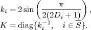
Theorem 5.2 Let ![]() , be diverse delays. System (5.4)–(5.5) is locally stable at the equilibrium point
, be diverse delays. System (5.4)–(5.5) is locally stable at the equilibrium point ![]() , if there exists a diagonal positive real number matrix
, if there exists a diagonal positive real number matrix ![]() such that
such that
(5.9) 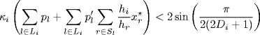
holds for all ![]() .
.
Obviously, Conjecture 5.1 is just a special case of Theorem 5.2 because when H is taken as the identity matrix, i.e. H = I, Theorem 5.2 reduces to Conjecture 5.1. This criterion of stability preserves the elegant property being locally implemented of Conjecture 5.1. Moreover, Theorem 5.2 enlarges the stability region for control gains and admissible delay constants.
Proof of Theorem 5.2. Define
![]()
Then, linearizing system (5.4)–(5.5) about the equilibrium point x* yields
(5.10) 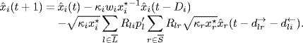
Assume the initial state of the linearized system is zero, ![]() for
for ![]() . Then, taking the z-transform, we obtain
. Then, taking the z-transform, we obtain
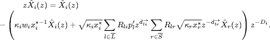
where ![]() is the z-transform of
is the z-transform of ![]() . Define the following matrices:
. Define the following matrices:
(5.13) ![]()
(5.14) ![]()
(5.15) ![]()
(5.16) ![]()
Then, (5.11) can be rewritten as
(5.18) ![]()
The characteristic equation of the above closed-loop system is
(5.19) ![]()
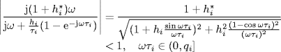
Now, we see that system (5.4)–(5.5) is locally stable at the equilibrium point, if all the roots of the characteristic equation have modulus less than unity. Note that
![]()
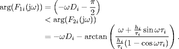
has no poles outside the unit disk in the complex plane (the pole z = 1 can be considered as inside the modified unit disk as shown by Figure 2.13). Therefore, by the generalized Nyquist criterion (Theorem 2.22), system (5.4)–(5.5) is locally stable, if the eigenloci of ![]() , i.e.,
, i.e., ![]() , do not enclose the point (− 1, j0) for all ω
, do not enclose the point (− 1, j0) for all ω ![]() [− π, π].
[− π, π].
Now, let us rewrite ![]() as
as
![]()
where
Obviously,
By the definition of M(z) given by (5.17) we have
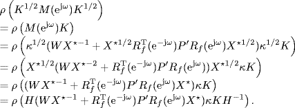
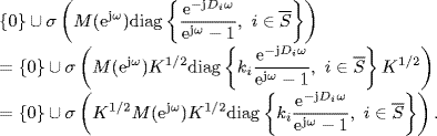
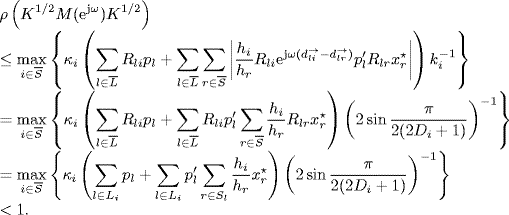
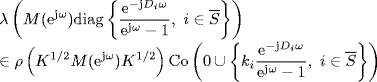
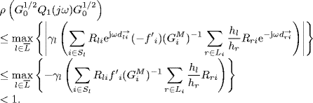
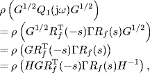
Recall that ![]() . By Corollary 2.31 of Gershgorin's disc lemma, the spectral radius of any matrix is bounded by its maximum absolute row sum. Therefore, by the definitions of all matrices (5.12)–(5.17) and the assumption of Theorem 5.2, we get
. By Corollary 2.31 of Gershgorin's disc lemma, the spectral radius of any matrix is bounded by its maximum absolute row sum. Therefore, by the definitions of all matrices (5.12)–(5.17) and the assumption of Theorem 5.2, we get
Then, by Vinnicombe's lemma (Lemma 2.34) we get
holds for all ω ![]() [− π, π].
[− π, π].
Now, we can see the problem has been converted to the scalability condition for the first-order time-delayed system of the form
![]()
This problem was solved in Chapter 3 (§3.3.2) by Theorem 3.16. Using this theorem we know that
![]()
does not contain the point (− 1, j0) when ![]() . And hence, the eigenloci
. And hence, the eigenloci ![]() cannot enclose the point (− 1, j0) for all ω
cannot enclose the point (− 1, j0) for all ω ![]() [− π, π]. The theorem is thus proved.
[− π, π]. The theorem is thus proved.
Theorem 5.2 preserves the elegant property of Conjecture 5.1 being decentralized and locally implemented: each end system needs knowledge only of its own round-trip delay. Moreover, it enlarges the stability region of control gains and admissible communication delays.
From Theorem 5.2 we know that the stability region of control gain is given by ![]() where
where
![]()
Consider H as a parameter one can draw a curved surface κ(H) in the gain space. The stability region is covered by this curved surface and bounded by κi > 0. However, Conjecture 5.1 suggests that the stability region is a hyper-rectangle given by ![]() , which is inside the region given by Theorem 5.2.
, which is inside the region given by Theorem 5.2.
Since ![]() is strictly monotone when Di ≥ 0, fixing control gains κi, we get from Theorem 5.2 the bounds of the admissible values of delay constants as follows
is strictly monotone when Di ≥ 0, fixing control gains κi, we get from Theorem 5.2 the bounds of the admissible values of delay constants as follows
where Ing(x) represents the function which maps x to the nearest integer towards infinity.
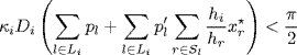
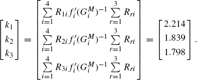
To illustrate the theoretic results we perform simulation as follows. We simulate a network with one link shared by three sources. The routing matrix is R = [1 1 1]. The congestion indication function is chosen as p(y) = 1 − ey(1 − y), where ![]() is the network load. Setting
is the network load. Setting ![]() we get the equilibrium of the transmission rate is x* = [0.0255, 0.0509, 0.0763]T by (5.3). Then we can calculate p and p′ at x*. We first fix the round-trip delay Di(i = 1, 2, 3) as 80(ms), 60(ms), and 70(ms). Then, scaling on the parameter matrix H = diag{h1, h2, h3} (for simplicity of calculation, h1 can always be taken as unity, i.e., h1 = 1), we can obtain a curved surface of the critical gains, κ*(H), shown in Figure 5.1. Setting κ3 = 0.0448, we get a two-dimensional transversal of κ*(H) as shown in Figure 5.2. In the figure, “Area(2)” is the stability region determined by Conjecture 5.1 while the entire area covered by the curve κ*(H) (“Area(1)”∪“Area(2)”∪“Area(3)”) is the stability region of control gains determined by Theorem 5.2.
we get the equilibrium of the transmission rate is x* = [0.0255, 0.0509, 0.0763]T by (5.3). Then we can calculate p and p′ at x*. We first fix the round-trip delay Di(i = 1, 2, 3) as 80(ms), 60(ms), and 70(ms). Then, scaling on the parameter matrix H = diag{h1, h2, h3} (for simplicity of calculation, h1 can always be taken as unity, i.e., h1 = 1), we can obtain a curved surface of the critical gains, κ*(H), shown in Figure 5.1. Setting κ3 = 0.0448, we get a two-dimensional transversal of κ*(H) as shown in Figure 5.2. In the figure, “Area(2)” is the stability region determined by Conjecture 5.1 while the entire area covered by the curve κ*(H) (“Area(1)”∪“Area(2)”∪“Area(3)”) is the stability region of control gains determined by Theorem 5.2.
Figure 5.1 The curved surface of critical gains.
Figure 5.2 Stability region of control gains.
Similarly, for a fixed [κ1, κ2, κ3] = [0.0527, 0.0588, 0.0448] we can also obtain the range of values of the admissible delays. Its two-dimensional transversal at D3 = 70(ms) is shown in Figure 5.3, where “Area(2)” is the range of values of admissible delays determined by Conjecture 5.1, and “Area(1)” ∪ “Area(2)” ∪ “Area(3)” is the range of values of admissible delays determined by Theorem 5.2.
Figure 5.3 Range of admissible delays.
5.1.3 Scalable Stability Criterion for Continuous-Time Systems
The continuous-time version of system (5.4)–(5.5) is given by

Then, an analog of Conjecture 5.1 for the continuous-time system (5.20)–(5.21) can be stated as follows (Vinnicombe (2000).
Conjecture 5.2 Let![]() , be diverse round-trip delays. System (5.20)–(5.21) is locally stable at the equilibrium point x*, if
, be diverse round-trip delays. System (5.20)–(5.21) is locally stable at the equilibrium point x*, if
(5.22) 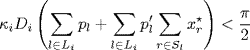
holds for all ![]() , where
, where
(5.23) 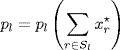
and pl′ is the derivative of pl evaluated at ![]() , i.e.,
, i.e.,
(5.24) 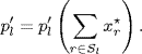
Massoulie (2002) proved a weaker version of Conjecture 5.3, which says that system (5.20)–(5.21) with diverse round-trip delays is locally stable at the equilibrium point, if
(5.25) 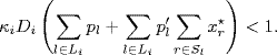
Similar to the derivation for the discrete-time model, we can prove the following theorem which includes Conjecture 5.3 as a special result.
Theorem 5.4 Let ![]() , be diverse round-trip delays. System (5.20)–(5.21) is locally stable at the equilibrium point x*, if there exists a diagonal positive real number matrix
, be diverse round-trip delays. System (5.20)–(5.21) is locally stable at the equilibrium point x*, if there exists a diagonal positive real number matrix ![]() such that
such that
holds for all ![]() .
.
Proof. Similar to the proof of Theorem 5.2 we can show that system (5.21)–(5.21) is locally stable at the equilibrium point if
holds for all ω ![]() (− ∞, ∞). So, the proof of the theorem is converted to the scalability condition for the first-order continuous-time system of the form
(− ∞, ∞). So, the proof of the theorem is converted to the scalability condition for the first-order continuous-time system of the form
![]()
This problem has been solved in Chapter 3 (§3.3.1) by Theorem 3.10. Using this theorem we know that (5.27) holds for all ω ![]() (− ∞, ∞) if
(− ∞, ∞) if ![]() , which is ensured by (5.26). The theorem is thus proved.
, which is ensured by (5.26). The theorem is thus proved.
Exercises 5.5 Consider the system with dual algorithm (4.32)–(4.35). Prove that under diverse round-trip delays ![]() , the system is locally stable about the equilibrium point, if there exists a diagonal positive real matrix
, the system is locally stable about the equilibrium point, if there exists a diagonal positive real matrix ![]() such that
such that
(5.28) ![]()
holds for all ![]() , where fi′ is the derivative of the function Ui′ −1(·) at the equilibrium point.
, where fi′ is the derivative of the function Ui′ −1(·) at the equilibrium point.
Exercises 5.6 Derive the expression of the equilibrium point, linearized the model and scalable local stability condition of the time-delayed primal algorithm given by (4.28)–(4.31).
5.2 Stability of REM
By doing Exercise 5.5, one can see that the scalable stability results of the primal algorithm also exist for the dual algorithm, thanks to the symmetry between the primal algorithm and the dual algorithm. This may give the reader an impression that the Johari–Tan-like results may hold for other distributed congestion control algorithms. To give a more clear insight into this problem we study the stability of the second-order AQM control algorithm: REM. This control scheme was first proposed by Athuraliya, Low and Yin (2001) to overcome the drawback of the first-order dual algorithm that prices are proportional to link backlogs and thus the equilibrium can have large backlogs. Note that this algorithm is globally stable in the absence of communication delays (Paganini (2002). The local stability of the algorithm with one link or identical round-trip delay was studied in Yin and Low (2001), (2002). In this section we use the frequency-domain approach to analyze the stability of the REM algorithm in the presence of diverse round-trip delays.
5.2.1 Scalable Stability Criteria
The continuous-time version of the REM algorithm is given by (Paganini (2002)
where ![]() is the price (congestion measurement) at link l; γl > 0 the control gains;
is the price (congestion measurement) at link l; γl > 0 the control gains; ![]() the aggregate rate at link l; cl the capacity of link l;
the aggregate rate at link l; cl the capacity of link l; ![]() some internal variable for the price control, which often represents the queue length in the buffer of link l; el some desired value for the queue length at link l.
some internal variable for the price control, which often represents the queue length in the buffer of link l; el some desired value for the queue length at link l.
Note that unlike Paganini (2002) in which all the links share a common control gain, i.e., ![]() , here we assume that each link may have its own control gain. However, for the semi-homogeneousness of the system we assume that all the links have the same dynamics, and consequently, the control parameters αl for the links in (4.23) take the same value, i.e.,
, here we assume that each link may have its own control gain. However, for the semi-homogeneousness of the system we assume that all the links have the same dynamics, and consequently, the control parameters αl for the links in (4.23) take the same value, i.e., ![]() .
.
The transmitting rate at each source is generated by the following function:
where Ui′ −1(qi) is the inverse of the derivative of Ui(qi), a utility function which is assumed to be differentiable and strictly concave. Hence, fi(qi) is a strictly monotonically decreasing function of qi.
For a given link ![]() and each source i
and each source i ![]() Sl, there is a forward delay
Sl, there is a forward delay ![]() of delivering packets from source i to link l, and a backward delay
of delivering packets from source i to link l, and a backward delay ![]() of sending the feedback signal from link l to source i. Note that each route is subject to a round-trip delay Di satisfying (4.27). Under propagation delays the following relationships are immediate:
of sending the feedback signal from link l to source i. Note that each route is subject to a round-trip delay Di satisfying (4.27). Under propagation delays the following relationships are immediate:
(5.32) ![]()
Equations (5.29)–(5.33) constitute a dynamical feedback system which has a unique equilibrium (b*, p*) satisfying
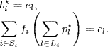
For convenience, in the further development we denote
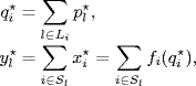
as the aggregate price of all links used by source i and the aggregate rate of all sources which use link l at the equilibrium, respectively. The vectors ![]() are defined by the above components across the set of sources (links).
are defined by the above components across the set of sources (links).
We have assumed that the desired value of the queue length at each link is positive, i.e., ![]() . Therefore, in the neighborhood of (b*, p*), the system (5.29)–(5.30) is differentiable and simply governed by
. Therefore, in the neighborhood of (b*, p*), the system (5.29)–(5.30) is differentiable and simply governed by
(5.34) ![]()
For simplicity of statement, we call the system consisting of equations (5.31)–(5.35) as “system ∑rem”.
Define
where f′ i is the derivative of the function fi(·) at the equilibrium point. Note that f′ i < 0 because fi(·) is a strictly monotonically decreasing function.
Then, we can linearize system ∑rem about the equilibrium point and get
Let ![]() , the Laplace transformation of
, the Laplace transformation of ![]() . The closed-loop system (5.36) can be represented in the Laplace domain as follows:
. The closed-loop system (5.36) can be represented in the Laplace domain as follows:
Denote
(5.38) ![]()
(5.39) ![]()
(5.40) ![]()
(5.41) ![]()
where ![]() is the round-trip delay of the route associated with source i. Then, by using the relationship between the forward routing matrix and the backward routing matrix (4.72), equation (5.37) can be rewritten in the following matrix form:
is the round-trip delay of the route associated with source i. Then, by using the relationship between the forward routing matrix and the backward routing matrix (4.72), equation (5.37) can be rewritten in the following matrix form:
The characteristic equation of the above closed-loop system is
Now, we see that system ∑rem is locally stable, if all the roots of the characteristic equation have negative real parts.
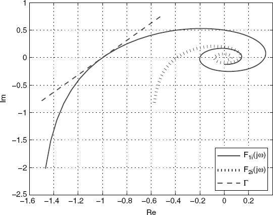
Before presenting our stability result for the general case, let us consider a special case when only one link and one source are involved in the network. In this case, the diagram of the closed-loop system (5.42) is shown in Figure 5.4.
Let D = d→ + d←, and
(5.44) ![]()
Figure 5.4 Closed-loop system of congestion control.
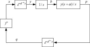
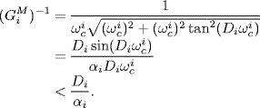
Denote by GM the gain margin of W(s) which is defined by
(5.45) ![]()
where ωc > 0 is the frequency at which the phase of W(jω) is equal to π. ωc is the minimal crossing frequency of W(jω) because the Nyquist plot of W(jω) crosses the real axis of the complex plane for the first time at ω = ωc, i.e., ωc is the minimal frequency satisfying
(5.46) ![]()
According to the Nyquist criterion of stability (Theorem 2.20), we know that the closed-loop system shown in Figure 5.4 is asymptotically stable if and only if
(5.47) ![]()
Now, let us consider the general case when S sources and L links are involved in the network. For each ![]() we denote
we denote
(5.48) ![]()
Let ![]() be the source which has the maximal round-trip delay, i.e.,
be the source which has the maximal round-trip delay, i.e.,
We make the assumption on the control parameter and the delays of the network as follows.
Assumption 5.7
Now, we are in a position to present the following stability result.
Theorem 5.8 Under Assumption 5.7, the system ∑rem is locally stable about the equilibrium point (b*, p*), if there exists a diagonal positive real matrix ![]() such that
such that
holds for all ![]() , where
, where ![]() is the gain margin of the transfer function
is the gain margin of the transfer function
![]()
In particular, when H is taken as the identity matrix, the stability condition reduces to
Proof. To prove the theorem let us return to equation (5.43). According to Theorem 2.20, all the roots of the characteristic equation (4.79) have negative real parts if and only if the eigenloci of ![]() , i.e.,
, i.e.,
![]()
do not enclose the point (− 1, j0) for all ω ![]() [0, ∞), where λ(·) denotes the matrix eigenvalue.
[0, ∞), where λ(·) denotes the matrix eigenvalue.
Let us rewrite matrix
![]()
as ![]() , where
, where
(5.53) ![]()
(5.54) ![]()
(5.55) ![]()
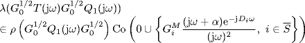
By the definition of Q1(s) we have
Recall that ![]() . By Corollary 2.31 of Gershgorin's disc lemma, the spectral radius of any matrix is bounded by its maximum absolute column sum. Therefore, from (5.51) we get
. By Corollary 2.31 of Gershgorin's disc lemma, the spectral radius of any matrix is bounded by its maximum absolute column sum. Therefore, from (5.51) we get
Note that ![]() . Therefore, it follows from Vinnicombe's lemma (Lemma 2.34) that
. Therefore, it follows from Vinnicombe's lemma (Lemma 2.34) that
holds for all ω ![]() [0, ∞).
[0, ∞).
Now, we see that the proof of the theorem has been converted to the problem of the scalability of the second-order time-delayed system of type II
The problem has been solved in Chapter 3 (§3.4.2) by Theorem 3.32. According to this theorem,
![]()
does not contain the point (− 1, j0) when ![]() . And hence, the eigenloci
. And hence, the eigenloci ![]() do not enclose the point (− 1, j0) for all ω
do not enclose the point (− 1, j0) for all ω ![]() [0, ∞). The theorem is thus proved.
[0, ∞). The theorem is thus proved.
Remark 1. The clockwise property of the frequency response function of a time-delayed congestion control system plays a key role in obtaining scalable stability criteria such as Johari and Tan's conjecture as well as Theorem 5.2. Unfortunately, when a congestion control algorithm has a second-order dynamical law such as the REM algorithm, this clockwise property does not hold in the whole frequency band. Theorem 5.8, together with Theorem 3.32, indicates that if the network parameters satisfies Assumption 5.7, the clockwise property still holds in a certain frequency interval, and a scalable stability criteria can still be established for the REM algorithm.
Remark 2. The introduction of the diagonal matrix H can balance the control gains among link nodes and make the stability condition less conservative.
Remark 3. It can be shown that ![]() increases while Di increases. So, roughly speaking,
increases while Di increases. So, roughly speaking, ![]() represents the size of the round-trip delay constant Di. Therefore, the inequality (5.51) or (5.52) given by Theorem 5.8 can be regarded as a specification of the relationship between the control gain at a link and the weighted sum of the round-trip delay constants of the sources using the link. So the inequality (5.51) or (5.52) is useful for determining the control gain of each link if the round-trip delay constants are known.
represents the size of the round-trip delay constant Di. Therefore, the inequality (5.51) or (5.52) given by Theorem 5.8 can be regarded as a specification of the relationship between the control gain at a link and the weighted sum of the round-trip delay constants of the sources using the link. So the inequality (5.51) or (5.52) is useful for determining the control gain of each link if the round-trip delay constants are known.
The next theorem gives a dual stability condition for REM algorithm. The inequality provided by this theorem can be used for evaluating the maximal admissible round-trip delay constant of each source when all the control gains at links are already fixed.
Theorem 5.9 Under Assumption 5.7, the system ∑rem is locally stable about the equilibrium point (b*, p*), if there exists a diagonal positive real matrix ![]() such that
such that
holds for all ![]() . In particular, when H is taken as the identity matrix, the stability condition reduces to
. In particular, when H is taken as the identity matrix, the stability condition reduces to
![]()
Proof. The spectral radius of any matrix is also bounded by its maximum absolute row sum. So, from (5.57) one can also get ![]() . The rest of the proof is similar to the proof of Theorem 5.8.
. The rest of the proof is similar to the proof of Theorem 5.8.
5.2.2 Dual Algorithm: the First-Order Limit Form of REM
From Theorem 5.8 or Theorem 5.9 it is easy to derive stability conditions for the first-order dual algorithm. If the control parameters ![]() in equation (4.23) are all set to be zero, the second-order dual algorithm reduces to the first-order one. In this case we note that
in equation (4.23) are all set to be zero, the second-order dual algorithm reduces to the first-order one. In this case we note that ![]() and, therefore, Assumption 5.7 is automatically satisfied for any delay constants Di. In this case, the open-loop transfer function for source i becomes
and, therefore, Assumption 5.7 is automatically satisfied for any delay constants Di. In this case, the open-loop transfer function for source i becomes
And it is easy to know that the gain margin for this transfer function is
![]()
Therefore, we get the following results just as corollaries of Theorem 5.8 and Theorem 5.9 for the first-order dual algorithm.
Theorem 5.10 Suppose α = 0. Then the system ∑rem is locally stable about the equilibrium point, if there exists a diagonal positive real matrix ![]() such that
such that
holds for all ![]() . In particular, when H is taken as the identity matrix, the stability condition reduces to
. In particular, when H is taken as the identity matrix, the stability condition reduces to
(5.61) ![]()
Theorem 5.11 Suppose α = 0. Then the system ∑rem is locally stable about the equilibrium point, if there exists a diagonal positive real matrix ![]() such that
such that
holds for all ![]() . In particular, when H is taken as the identity matrix, the stability condition reduces to
. In particular, when H is taken as the identity matrix, the stability condition reduces to
(5.63) ![]()
Remark. In the REM algorithm, there are mainly two kinds of parameters to be designed, namely, control gains γl and parameter α. Note that 1/α can be viewed as the time constant of differentiation in the open-loop transfer function (5.56). While the relationship between the control gains and the round-trip delay constants is basically specified by condition (5.51) or (5.57), as explained in Remark 3 on Theorem 5.8, the relationship between the time constant of differentiation 1/α and the round-trip delay constants is basically described by Assumption 5.7. The assumption implies that when the maximal round-trip delay in the network is large, the time constant of differentiation 1/α should be also large (consequently, α should be small) so that delay effect can be overcome by the prediction effect of the differentiation operator. From (5.59) it is easy to see that when α is very small and approaches zero, the dynamics of REM algorithm is very similar to those of the first-order AQM algorithm, the stability of which is determined only by the scalable gain condition (5.60) or (5.62). However, this does not imply that the steady performance (equilibrium property) of the REM algorithm is also similar to that of the first-order AQM algorithm. Even in the case when α approaches zero (but not equal to zero), the REM algorithm still has the merit that the link backlogs are small at the equilibrium point.
5.2.3 Design of Parameters of REM
Now, we propose a simple scheme for designing the parameters of the REM algorithm with the purpose of guaranteeing the local asymptotic stability.
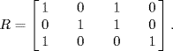
Let us illustrate the design procedure using a network with three links shared by four sources, which is shown in Figure 5.5. The routing matrix of this network is given by
Let the round-trip delays associated with the sources be D1 = 1.1(s), D2 = 1.0(s), D3 = 0.8(s), D4 = 0.7(s). According to (5.50), we know that ![]() in this network. Our purpose is to design the control parameter α and the control gains γl, l = 1, 2, 3, to guarantee the local asymptotic stability of the REM algorithm. Based on Theorem 5.8, the design procedure can be sketched as follows.
in this network. Our purpose is to design the control parameter α and the control gains γl, l = 1, 2, 3, to guarantee the local asymptotic stability of the REM algorithm. Based on Theorem 5.8, the design procedure can be sketched as follows.
![]()
![]()
![]()
![]()
Figure 5.5 A network controlled by REM.
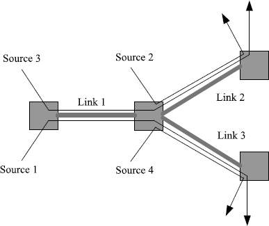
Figure 5.6 Design of parameters by Assumption 5.7 (A1). (Reproduced with permission from Tian Y.-P., “Stability analysis and design of the second-order congestion control for networks with heterogeneous delays,” IEEE/ACM Transactions on Networking, 13, 5, 1082–1093, 2005. © 2005 IEEE.)
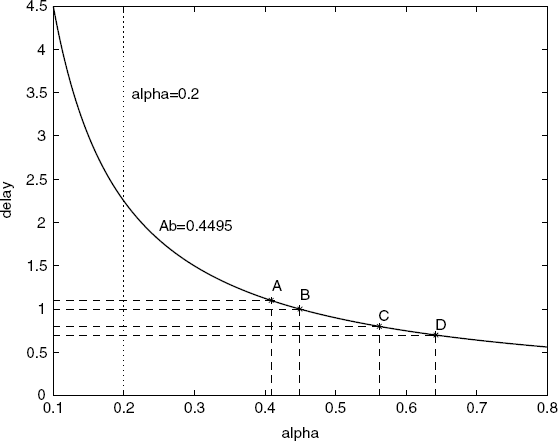
Figure 5.7 Design of parameters by Assumption 5.7 (A2). (Reproduced with permission from Tian Y.-P., “Stability analysis and design of the second-order congestion control for networks with heterogeneous delays,” IEEE/ACM Transactions on Networking, 13, 5, 1082–1093, 2005. © 2005 IEEE.)
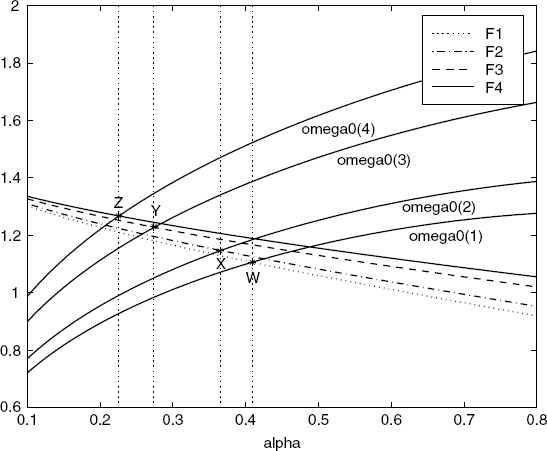
Figure 5.8 The Nyquist plots of round-trip dynamics. (Reproduced with permission from Tian Y.-P., “Stability analysis and design of the second-order congestion control for networks with heterogeneous delays,” IEEE/ACM Transactions on Networking, 13, 5, 1082–1093, 2005. © 2005 IEEE.)
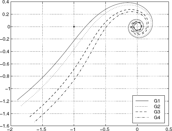
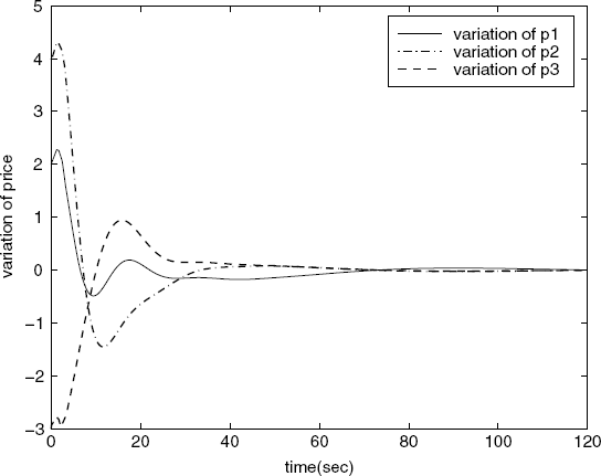
Figure 5.9 Variation of prices around the equilibrium. (Reproduced with permission from Tian Y.-P., “Stability analysis and design of the second-order congestion control for networks with heterogeneous delays,” IEEE/ACM Transactions on Networking, 13, 5, 1082–1093, 2005. © 2005 IEEE.)
It is interesting to point out that, unlike the first-order control algorithm, condition (5.51) or condition (5.52) is not sufficient for the local stability of the second-order control algorithm. This can be shown by the following counter-example. We assume the round-trip delay D4 in the above setting is changed from 0.7(s) to 0.02(s), and the parameters ![]() are now set as
are now set as ![]() ,
, ![]() ,
, ![]() ,
, ![]() . All the other parameters including the control gains are the same as given previously. Then, one can get the source rates and the aggregate prices at the equilibrium as
. All the other parameters including the control gains are the same as given previously. Then, one can get the source rates and the aggregate prices at the equilibrium as ![]() (Mbps),
(Mbps), ![]() (Mbps),
(Mbps), ![]() (Mbps),
(Mbps), ![]() (Mbps),
(Mbps), ![]() ,
, ![]() ,
, ![]() ,
, ![]() . Therefore, the equilibrium values of derivatives of the inverse utility functions of the sources,
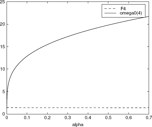
. Therefore, the equilibrium values of derivatives of the inverse utility functions of the sources, ![]() , are f′ 1 = − 0.7, f′ 2 = − 1.03, f′ 3 = − 0.82, f′ 4 = − 115, respectively. It is easy to verify that condition (5.52) still holds for this new setting. But the variation of the price at link 3 goes to infinity as shown in Figure 5.10. The reason for this is perhaps that the condition (A2) of Assumption 5.7 does not hold any more for ω0(4) in this case (see Figure 5.11).
, are f′ 1 = − 0.7, f′ 2 = − 1.03, f′ 3 = − 0.82, f′ 4 = − 115, respectively. It is easy to verify that condition (5.52) still holds for this new setting. But the variation of the price at link 3 goes to infinity as shown in Figure 5.10. The reason for this is perhaps that the condition (A2) of Assumption 5.7 does not hold any more for ω0(4) in this case (see Figure 5.11).
Figure 5.10 Counter-example: Variation of prices around the equilibrium. (Reproduced with permission from Tian Y.-P., “Stability analysis and design of the second-order congestion control for networks with heterogeneous delays,” IEEE/ACM Transactions on Networking, 13, 5, 1082–1093, 2005. © 2005 IEEE.)
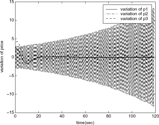
Figure 5.11 Counter-example: Prerequisite 2 does not hold. (Reproduced with permission from Tian Y.-P., “Stability analysis and design of the second-order congestion control for networks with heterogeneous delays,” IEEE/ACM Transactions on Networking, 13, 5, 1082–1093, 2005. © 2005 IEEE.)
5.3 Stability of the Primal-Dual Algorithm
In the last chapter we showed that the primal algorithm allows general utility functions, hence arbitrary fairness in rate allocation, but gives up tight control on utilization, whereas the dual algorithm can achieve very high utilization but is restricted to a specific class of utility functions. The primal-dual algorithm adopts dynamical adaptations both at links and at sources, and can achieve both high utilization and arbitrary fairness. In this section we will establish some stability criteria for the primal-dual algorithm with diverse round-trip delays.
5.3.1 Scalable Stability Criteria
Consider the following primal-dual algorithm which has dynamics at both source end and link end:
where ![]() , ki > 0 are the transmission rate and control gain at source i,
, ki > 0 are the transmission rate and control gain at source i, ![]() , respectively;
, respectively; ![]() , γl > 0 are the price (congestion measurement) and control gain at link l,
, γl > 0 are the price (congestion measurement) and control gain at link l, ![]() , respectively;
, respectively; ![]() is the desired aggregate equilibrium rate on link l; and Ui′ (xi) is the derivative of Ui(xi), a utility function.
is the desired aggregate equilibrium rate on link l; and Ui′ (xi) is the derivative of Ui(xi), a utility function.
Similar to any other congestion control algorithm with propagation delays, we have equations which describe the interconnection of the sources and links:
where the forward delay ![]() and backward
and backward ![]() are subject to the well known assumption (4.27), which says all the links associated with the same route have the same round-trip delay.
are subject to the well known assumption (4.27), which says all the links associated with the same route have the same round-trip delay.
Equations (5.66)–(5.69) constitute a dynamical feedback system with a unique equilibrium (x*, p*) satisfying
For convenience in the following discussions, we denote

as the aggregate price of all links used by source i and the aggregate rate of all sources which use link l at the equilibrium, respectively. The vectors ![]() are defined by the above components across the set of sources or links in an obvious way.
are defined by the above components across the set of sources or links in an obvious way.
Next, we study the local stability of the equilibrium (x*, p*) in the presence of delays. In a neighborhood of (x*, p*), the system (5.66)–(5.67) is differentiable and simply governed by
For simplicity of statement, we call the system consisting of equations (5.68), (5.69), (5.71) and (5.72) “system ∑pd”.
Define
Then, we can linearize system ∑pd about the equilibrium point and get
where ![]() is the derivative of Ui′ (xi) at
is the derivative of Ui′ (xi) at ![]() .
.
Remark. In last chapter, we considered a generalized form of the primal-dual algorithm where the control gains ki in (5.66) a non-decreasing function of the transmission rate ki(xi). In that case the linearized equations about the equilibrium point are
(5.74) 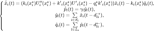
which have the same form as (5.73). So, the results given in this section also apply to the generalized form of the primal-dual algorithm.
Let ![]() , the Laplace transformation of
, the Laplace transformation of ![]() . Then, the closed-loop system (5.73) can be represented in the Laplace domain as follows:
. Then, the closed-loop system (5.73) can be represented in the Laplace domain as follows:
Denote
(5.76) ![]()
(5.77) ![]()
(5.78) ![]()
where
Then, by using the relationship between the time-delayed forward and backward routing matrices (4.72), equation (5.75) can be rewritten in the following matrix form:
(5.80) ![]()
where Rf(s) is the time-delayed forward routing matrix. The characteristic equation of the above system is
Now, we see that system ∑pd is locally stable, if all the roots of the characteristic equation have negative real parts.
Denote by ![]() the gain margin of the transfer function
the gain margin of the transfer function
(5.82) ![]()
which is defined by
(5.83) ![]()
where ![]() is the minimal frequency that satisfies the following equation:
is the minimal frequency that satisfies the following equation:
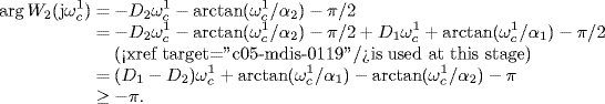
Note that the locus of Wi(jω) crosses the real axis of the complex plane for the first time when ![]() , which is the minimal crossing frequency of Wi(jω).
, which is the minimal crossing frequency of Wi(jω).
From (5.84) we have
![]()
Using this equality, we get
The following theorem gives some sufficient conditions for the asymptotic stability of the primal-dual algorithm.
Theorem 5.12 Suppose that the following precondition holds for the primal-dual algorithm:
Then system ∑pd is locally stable about the equilibrium point (x*, p*), if there exists a diagonal positive real matrix ![]() such that
such that
or, if there exists a diagonal positive real matrix ![]() such that
such that
Remark 1. Inequality (5.87) or (5.88) is a scalable stability condition, which does not require knowledge of the entire network. A precondition for the validity of such a scalable condition is that (5.86) holds. Therefore, equation (5.86) can be regarded as a scalability condition of the primal-dual algorithm.
Remark 2. As we have remarked before, the introduction of the diagonal matrix H (or H′) can balance the control gains among source (or link) nodes and make the stability conditions less conservative. If H is taken as the identity matrix, condition (5.87) reduces to
(5.89) ![]()
Using (5.79) and (5.85), we can further get a more explicit sufficient condition than (5.87) as
Similarly, we can get an explicit sufficient condition, simpler than (5.88), as
A sufficient condition for the scalability condition (5.86), which is checked only by round-trip delays and the algorithm parameter α, is given by the following proposition.
Proposition 5.13 Condition (5.86) holds if
Proof. Suppose (5.92) holds for i, j = 1, 2. Without loss of generality, we assume D1α1 − D2α2 ≤ 0. Then, (5.92) implies that D1 ≥ D2 and α1 ≤ α2. To show that (5.86) holds, we only need to show ![]() , or equivalently,
, or equivalently,
(5.93) ![]()
Indeed,
The last inequality holds because ![]() when α1 ≤ α2.
when α1 ≤ α2.
Now, we give a simple example to illustrate the design of the parameter α and control gains in the primal-dual algorithm with the help of the scalability and stability conditions.
Example 5.14 Design of parameters of the primal-dual algorithm.
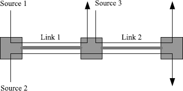
Consider the simple network with two links and three sources, which is illustrated by Figure 5.12. Source 2's route includes link 1 and link 2, source 1's route consists of link 1 and source 3's route consists of link 2. Obviously, the routing matrix of the network is
![]()
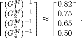
Let the round-trip delays associated with the sources be D1 = 1(s), D2 = 0.7(s), D3 = 0.4(s). Assume that the link capacities are c1 = 3(Mbps), c2 = 2(Mbps), and the desired aggregate rates on links are equal to the link capacities, i.e., ![]() ,
, ![]() . The utility function is
. The utility function is ![]() , where the parameter
, where the parameter ![]() is set to unity for each source. Then, from (5.70) it is easy to get the equilibrium point of the network as
is set to unity for each source. Then, from (5.70) it is easy to get the equilibrium point of the network as
![]()
The control gains of sources and links can be designed as follows.
Figure 5.12 Network with two links and three sources.
![]()
![]()
Figure 5.13 Source rates. (Reprinted from Tian Y.-P. and Chen G., “Stability of the primal-dual algorithm for congestion control,” International Journal of Control, 79, 6, 662–676, © 2006, by permission of Taylor & Francis Ltd, http://www.tandf.co.uk/journals.)
Figure 5.14 Link prices. (Reprinted from Tian Y.-P. and Chen G., “Stability of the primal-dual algorithm for congestion control,” International Journal of Control, 79, 6, 662–676, © 2006, by permission of Taylor & Francis Ltd, http://www.tandf.co.uk/journals.)
The above example shows that the scalability requirement and stability condition can usually be met by adjusting the control gains at the sources. When this is not the case, to maintain the local asymptotic stability we can strengthen condition (5.87) as described in the rest of this section.
Let
(5.94) ![]()
Denote by ![]() the source with minimal value of parameter Ai, i.e.,
the source with minimal value of parameter Ai, i.e.,
(5.95) ![]()
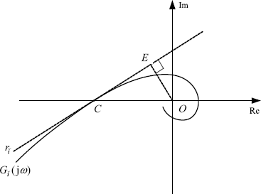
Let ![]() be the slope of the tangent line to the Nyquist plot of
be the slope of the tangent line to the Nyquist plot of ![]() at the intersection point C, as illustrated by Figure 5.15. It is easy to see that
at the intersection point C, as illustrated by Figure 5.15. It is easy to see that ![]() . An analytic formula of
. An analytic formula of ![]() is given by
is given by
(5.96) ![]()
Define
(5.97) 
Now, we are ready to give an alternative theorem for the local asymptotic stability of the primal-dual algorithm.
Figure 5.15 Tangent line of Nyquist plot.
Theorem 5.15 System ∑pd is locally stable about the equilibrium point (x*, p*), if there exists a diagonal positive real matrix ![]() such that
such that
or, if there exists a diagonal positive real matrix ![]() such that
such that
Remark. Using (5.79) and (5.85), we can get some more explicit sufficient conditions from (5.98) and (5.99) as
and
(5.101) ![]()
respectively. Compared to (5.90) or (5.91) given by Theorem 5.12, these conditions are sufficient for the stability of the primal-dual algorithm without preconditions. Condition (5.100) is almost scalable in the following sense: although the stability bound (μi in (5.100)) should be determined globally by considering all the routes in the network, actually the condition can be met by adjusting control parameters surrounding the sources so that the left-hand side of (5.100) is sufficiently small.
5.3.2 Proof of the Stability Criteria
Now, let us outline the procedure of the proofs of Theorems 5.12 and 5.15 As we show below, to close this proof procedure we need to use the geometric property of the frequency response function of the congestion control algorithm, which has been studied Chapter 3 in detail.
Proof of Theorem 5.12.
First, recall (5.81). According to the generalized Nyquist criterion (Theorem 2.20), all the roots of the characteristic equation (4.79) have negative real parts if and only if the eigenloci of
![]()
i.e., ![]() , do not enclose the point (− 1, j0) for all ω
, do not enclose the point (− 1, j0) for all ω ![]() [0, ∞).
[0, ∞).
Rewrite matrix
![]()
as G1/2T(s)G1/2Q1(s), where
(5.104) ![]()
By the definition of Q1(s), we have
where ![]() . It is well known that the spectral radius of a matrix is bounded by the maximum absolute value of its row sum. Therefore, by (5.87) we get
. It is well known that the spectral radius of a matrix is bounded by the maximum absolute value of its row sum. Therefore, by (5.87) we get
Since
![]()
it follows from Lemma 2.34 that
holds for all ω ![]() [0, ∞).
[0, ∞).
Now, by Theorem 3.23, under the condition (5.86),
![]()
does not contain the point (− 1, j0) when ![]() . Hence, the eigenloci
. Hence, the eigenloci
![]()
will not enclose the point (− 1, j0) for all ω ![]() [0, ∞). Thus, we have proved the sufficiency of (5.87) for the asymptotic stability of system ∑pd under precondition (5.86).
[0, ∞). Thus, we have proved the sufficiency of (5.87) for the asymptotic stability of system ∑pd under precondition (5.86).
Note that the spectral radius of a matrix is also bounded by the maximum absolute value of its column sum. So, from (5.88) one also gets ![]() . Therefore, the sufficiency of (5.88) for the asymptotic stability of system ∑pd under precondition (5.86) can be proved in a similar way. Theorem 5.12 is thus proved.
. Therefore, the sufficiency of (5.88) for the asymptotic stability of system ∑pd under precondition (5.86) can be proved in a similar way. Theorem 5.12 is thus proved.
Proof of Theorem 5.15.
To prove Theorem 5.15, we first need to modify (5.102) and (5.103) as follows:
(5.105) ![]()
(5.106) ![]()
Then, in a way similar to the proof of Theorem 5.12, by using Theorem 3.24 instead of Theorem 3.23, we can prove Theorem 5.15.
5.4 Time-Delayed Feedback Control
This section briefly reviews various forms and stability results of time-delayed feedback control (TDFC).
5.4.1 Time-Delayed State as a Reference
We explain the basic idea of the TDFC as it was originally proposed for stabilizing unstable periodic orbits of chaotic systems.
Consider a controlled continuous-time system,
where ![]() is the system state,
is the system state, ![]() is a nonlinear vector-valued function, and
is a nonlinear vector-valued function, and ![]() is the control input to be designed.
is the control input to be designed.
If the uncontrolled system (5.107) with u(t) = 0 is chaotic, then there are an infinite number of unstable periodic orbits (UPOs) in its attractive region (the reader who is interested in chaotic dynamics is referred to the following general introductions: Moon 1987; Peitgen, Juml;rgens and Saupe 1993; Schuster 1984; Wiggins 1988). Let ![]() be an unstable T-periodic solution of the uncontrolled system, which satisfies
be an unstable T-periodic solution of the uncontrolled system, which satisfies
(5.108) ![]()
Since it is difficult to get analytical or even numerical expressions of the target orbit ![]() because of its instability, there is no explicit reference for the stabilization of
because of its instability, there is no explicit reference for the stabilization of ![]() . Pyragas (1992) proposed the following TDFC to solve the problem:
. Pyragas (1992) proposed the following TDFC to solve the problem:
where ![]() is a constant gain matrix to be designed. The initial value of the control system is given as u(t) = 0, x(t) = ϕ(t), ∀ t
is a constant gain matrix to be designed. The initial value of the control system is given as u(t) = 0, x(t) = ϕ(t), ∀ t ![]() [− T, 0]. Obviously, when the system trajectory converges to a T-periodic orbit, the feedback control term in (5.109) vanishes automatically. Therefore, it guarantees that the reached orbit is indeed an inherent solution of the original uncontrolled system. In such a controller the time-delayed state x(t − T) is used as a target reference.
[− T, 0]. Obviously, when the system trajectory converges to a T-periodic orbit, the feedback control term in (5.109) vanishes automatically. Therefore, it guarantees that the reached orbit is indeed an inherent solution of the original uncontrolled system. In such a controller the time-delayed state x(t − T) is used as a target reference.
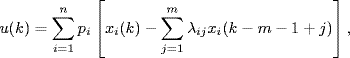
By simulations, Pyragas (1992) showed that by choosing an appropriate control gain K, the target UPO could be stabilized. Many experiments have confirmed this assertion (see, e.g., Ott, Simmendinger and Hess 1996; Parmananda, Madrigal and de Ciencias 1999). However, the theoretic research on TDFC shows that it is quite difficult to analyze the stability property of TDFC and, hence, it is also difficult to give analytic and effective methods for selecting the control gain (Just et al. 1997). Moreover, the domains of the control parameters over which the stabilization can be achieved are usually very small and limited so that the method generally fails to track higher-periodic orbits. To overcome the last problem, the original TDFC was soon being extended to the multiple-delay setting. Listed below are some versions of the extended TDFC (Basso, Genesio and Tesi 1997; Nakajima and Ueda 1998; Socolar et al. 1994):
where ![]() ;
;
where ![]() ;
;
where 0 ≤ ρ < 1. It is easy to verify that (5.110), (5.111) and (5.112) are essentially equivalent to each other. Notice also that ![]() when 0 ≤ ρ < 1. So, when m =∞ and μi = (1 − ρ)ρi−1, (5.111) reduces to (5.113).
when 0 ≤ ρ < 1. So, when m =∞ and μi = (1 − ρ)ρi−1, (5.111) reduces to (5.113).
When the measured signal is the system output ![]() instead of the system state, given by
instead of the system state, given by
(5.114) ![]()
the TDFC based on the output is
(5.115) ![]()
It is well know that an output feedback is not always as powerful as a state feedback in stabilization. The following dynamical output TDFC can be used for overcoming the limitation of the output TDFC:
where ![]() is the state of the observer system, and K1 and K2 are some gain matrices to be designed. A separation principle is proved for the dynamical output TDFC.
is the state of the observer system, and K1 and K2 are some gain matrices to be designed. A separation principle is proved for the dynamical output TDFC.
Theorem 5.16 (Tian and Chen (2001) The closed-loop system consisting of (5.107) and (5.116) is stable at the inherent T-periodic UPO if and only if the following two systems,
(5.117) ![]()
and
(5.118) ![]()
are both stable at the same UPO, where y(t) = h(x(t)) is the measured output of system (5.107).
The TDFC method can be easily extended to discrete-time systems. Suppose that for a nonlinear control system
![]() is a T-periodic UPO of the uncontrolled system, i.e.,
is a T-periodic UPO of the uncontrolled system, i.e.,
(5.120) ![]()
Then, the TDFC and extended TDFC for stabilizing Γ become
and
(5.122) ![]()
respectively.
5.4.2 TDFC for Stabilization of an Unknown Equilibrium
Let x* be an unstable fixed point (UFP) of the discrete-time system (5.119) without control, i.e.,
(5.123) ![]()
Since a UFP can be considered as a period one UPO, it may be stabilized by the one-step TDFC
The extended TDFC for stabilizing UFPs is given
(5.125) ![]()
Compared to conventional stabilization strategies, TDFC has an advantage that it does not need the value of the equilibrium point to be stabilized.
An equilibrium point of a continuous-time system can be considered as a trivial period orbit with arbitrary period. So the TDFC for stabilizing the equilibrium point of system (5.107) can be given as
where τ > 0 is called self-delay. Here, The self-delay τ is usually taken as some small constant in stabilization of equilibrium points (Kokame et al.(2001).
5.4.3 Limitation of TDFC in Stabilization
Ushio (1996) studied the stabilization of UFPs of discrete-time systems, and found that the TDFC is subject to a substantial limitation, which is now referred to as the odd number limitation. Later, the limitation of TDFC for continuous-time systems was also derived (Just et al. 1998; Nakajima 1997). After that, similar results were obtained for some other cases (Hino, Yamamoto and Ushio 2002; Kokame et al. 2001). Assume that the linearized system around the UFP x* is
(5.127) ![]()
where A = (∂/∂ x)f(x*, 0), B = (∂/∂ u)f(x*, 0), ![]() .
.
The odd number limitation for stabilizing UFPs of discrete-time systems is given by the following theorem.
Theorem 5.17 (Ushio (1996) If the Jacobian matrix A of system (5.119), evaluated at the target UFP x*, has an odd number of real eigenvalues that are greater than unity, then system (5.119) cannot be stabilized by the TDFC (5.124) at x* with any choice of the constant feedback gain matrix K.
Actually, if the real matrix A has an odd number of real eigenvalues that are greater than unity, then the following inequality holds:
![]()
It should be noted that the TDFC method also fails to stabilize UFPs in the case of det (I − A) = 0 (Yamamoto and Ushio (2003). So, the odd number limitation can be further modified as follows:
The proof of (5.128) is quite easy. Indeed, if the feedback control is taken as u = K[x(k) − x(k − 1)], then the linearized system of the closed-loop system is
It is obvious that the characteristic polynomial is
Since the controller ![]() should make the closed-loop system (5.129) stable, all the roots of (5.130) lie in the unit circle, which implies d(1) > 0 by the Jury stability criterion. Meanwhile, from (5.130) we can see that d(1) = det (I − A). Therefore, (5.128) is proved.
should make the closed-loop system (5.129) stable, all the roots of (5.130) lie in the unit circle, which implies d(1) > 0 by the Jury stability criterion. Meanwhile, from (5.130) we can see that d(1) = det (I − A). Therefore, (5.128) is proved.
Now, we consider the stabilization of a UPO. Assume that for nonlinear system (5.119) the linearized periodic time-varying system around the UPO Γ is
(5.131) ![]()
where ![]() ,
, ![]() ,
, ![]() . Write the state transition matrix for A(k) as
. Write the state transition matrix for A(k) as
(5.132) ![]()
The odd number limitation for stabilizing UPOs of discrete-time systems is then given by the following theorem.
Theorem 5.18 (Hino, Yamamoto and Ushio (2002) If the state transition matrix ΦA(T, 0) has an odd number of real eigenvalues that are greater than unity, then system (5.119) cannot be stabilized by the TDFC (5.121) at Γ with any choice of the constant feedback gain matrix K.
Actually, this limitation can also be generalized to the following form:
(5.133) ![]()
For the continuous-time system (5.107), assume that the linearized system around the equilibrium point x* is
(5.134) ![]()
where A = (∂/∂ x)f(x*, 0), B = (∂/∂ u)f(x*, 0), ![]() .
.
The odd number limitation for stabilizing equilibrium points of continuous-time systems is stated as follows.
Theorem 5.19 (Kokame et al. (2001) If the Jacobian matrix A of system (5.107), evaluated at the target equilibrium x*, has an odd number of real eigenvalues that are greater than zero, then the system (5.107) cannot be stabilized by the TDFC (5.126) at x* with any choices of the constant feedback gain matrix K and positive number τ.
Similarly, the generalized form of this limitation is
The assertion (5.135) can be easily proved as follows. If the feedback control is taken as u = K[x(t) − x(t − τ)], then the linearized system of the closed-loop system is
It is obvious that the characteristic polynomial is
Since the controller ![]() should make the closed-loop system (5.136) stable, all the roots of (5.137) lie in the open left-half plane, which implies d(0) > 0. Moreover, from (5.137) we can see d(0) = det (− A). Therefore, (5.135) is proved.
should make the closed-loop system (5.136) stable, all the roots of (5.137) lie in the open left-half plane, which implies d(0) > 0. Moreover, from (5.137) we can see d(0) = det (− A). Therefore, (5.135) is proved.
In the case of stabilizing a T-periodic UPO, the linearized system around the target UPO ![]() is
is
where ![]() ,
, ![]() are both T-periodic, and
are both T-periodic, and ![]() .
.
Using the Floquet theory for periodic systems, Nakajima (1997) proved the odd number limitation for stabilizing UPOs of continuous-time systems.
Theorem 5.20 (Nakajima (1997) If the linear variational equation (5.138) about the target hyperbolic UPO has an odd number of real characteristic multipliers greater than unity, then the UPO can not be stabilized by the TDFC with any choice of the constant feedback gain matrix K.
It follows from Theorem 5.16 that such a limitation also holds for the observer-based dynamic output TDFC method.
The odd number limitation discussed above describes a necessary condition for the stabilizability via TDFC or extended TDFC. In the discrete-time case, Ushio (1996) obtained a necessary and sufficient condition for the first-order and second-order controllable systems by using Jury's stability test. Up to now, necessary and sufficient conditions of stabilizability of TDFC are obtained only for single-input systems.
Consider an n-order nonlinear discrete-time system described by (5.119), where u(k) ![]() R is the control input,
R is the control input, ![]() is the state, and
is the state, and ![]() is a smooth mapping. Assume that x* is an unstable fixed point of the open-loop system, i.e., x* = f(x*, 0). Write A = (∂/∂ x)f(x*, 0) and b = (∂/∂ u)f(x*, 0). Then, TDFC of (5.124) reduces to a scalar form
is a smooth mapping. Assume that x* is an unstable fixed point of the open-loop system, i.e., x* = f(x*, 0). Write A = (∂/∂ x)f(x*, 0) and b = (∂/∂ u)f(x*, 0). Then, TDFC of (5.124) reduces to a scalar form
where ![]() .
.
A necessary and sufficient condition for the stabilizability via TDFC is given as follows.
Theorem 5.21 (Zhu and Tian (2005) Assume that (A, b) is controllable. There exists a TDFC in the form of (5.139) such that the closed-loop system of (5.119) is stable if and only if
Note that for n = 1 and n = 2, condition (5.140) is exactly the same as the results obtained by Ushio (1996).
Suppose that (A, b) is not controllable. Without loss of generality, let (A, b) be in the form of the following controllability decomposition:
![]()
Then, an extension of Theorem 5.21 can be given as follows.
Theorem 5.22 (Zhu and Tian (2005) The following statements are equivalent:
(5.141) ![]()
(5.142) ![]()
where n1 is the dimension of the controllable subspace of system (A, b), and θi (i = 1, 2, . . . , n − n1) are the uncontrollable poles of system (A, b).
Consider the extended TDFC
where λij ![]() R, satisfying
R, satisfying
(5.144) ![]()
and pi, i = 1, . . . , n, are control gains to be designed.
Then, a full characterization of the limitation of the extended TDFC is given as follows.
Theorem 5.23 (Tian and Zhu (2004) Assume that (A, b) is controllable. There exists an extended TDFC in the form of (5.143) such that the closed-loop system of (5.119) is stable if and only if
(5.145) ![]()
This result shows that the upper bound in the above-described condition can be enlarged by increasing the number of delays in the feedback. In other words, a system which cannot be stabilized by the conventional TDFC may still be stabilized by the extended TDFC, in contrast to the early claim that extended TDFC has no advantage over the conventional TDFC in overcoming the odd number limitation (Nakajima and Ueda (1998).
Kokame et al. (2001) considered the stabilization of equilibrium points for single-input continuous-time systems by applying TDFC, and showed that if the odd number limitation is excluded, then the UFP can be stabilized by TDFC.
Theorem 5.24 (Kokame et al. (2001) Assume that the linearized system of (5.107) about the target UFP, denoted (A, b), is controllable and det (− A) > 0. Then, there exists a pair of K and τ such the closed loop of (5.107) with TDFC (5.126) is locally asymptotically stable.
5.5 Stabilization of Congestion Control Systems by Time-Delayed Feedback Control
5.5.1 Introduction of TDFC into Distributed Congestion Control Systems
The basic idea of the congestion control is to adjust the sending rate of the source or decide the length of the queue in the buffer according to a certain algorithm in order to avoid congestion. Therefore, congestion control algorithms are usually classified into two types. One is implemented in TCP, which adjusts the data transmission windows at source nodes based on the congestion signal. The other is the AQM control strategy, which calculates the packet loss probability to adjust the queue length by detecting the queue in the buffer and judging the congestion circumstance in the network communication.
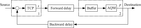
A network with congestion control algorithms (TCP and AQM) can be viewed as a closed-loop control system as shown in Figure 5.16. The feedback signal to the source is the congestion information from the link. The dashed frame 1 and the dashed frame 2 in the diagram correspond to the TCP algorithm at the source and the AQM strategy at the link, respectively, where x denotes the packets sending rate of the user and p denotes the congestion indication.
Figure 5.16 TCP-AQM as a closed loop control system.
Such a time-delayed feedback system may involve very complicated dynamics such as Hopf bifurcation (Li et al. 2004; Yang and Tian 2005) and chaos (Chen, Wang and Han 2004; Jiang, Wang and Xi 2004) when the stability conditions of a equilibrium point are destroyed. Moreover, the equilibrium point of a huge network varies with the change of the number of users and is not available for individual sources or links. Therefore, it is a natural idea to apply the TDFC method to the congestion control for enhancing the stability of the control algorithms.
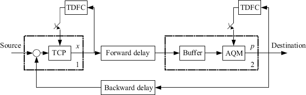
Figure 5.17 gives a kind of combination of the TDFC with currently used congestion control algorithms. In this framework the TDFC becomes active only if oscillations are detected in the network. The application of TDFC to the congestion control algorithm has the following advantages: (1) it does not need the steady state of the congestion algorithm; (2) it does not change the original algorithm and its steady state; (3) it can obtain various types of dynamical performance by adjusting the gain and the delay time of the TDFC.
Figure 5.17 Introduction of TDFC into congestion control.
5.5.2 Stabilizability under TDFC
Since a congestion control system is usually a time-delayed system, we first consider the following linear time-delayed system
where ![]() and
and ![]() are system matrices,
are system matrices, ![]() is the state,
is the state, ![]() is the control input,
is the control input, ![]() are delay constants. The following lemma shows the limitation of TDFC in the stabilization of such systems.
are delay constants. The following lemma shows the limitation of TDFC in the stabilization of such systems.
Lemma 5.25 Time-delayed system (5.146) can not be stabilized by the TDFC (5.126) if
![]()
Proof. The closed-loop form of system (5.146) with TDFC (5.126) is given by
(5.147) ![]()
where ![]() and τ > 0. The characteristic function is
and τ > 0. The characteristic function is
![]()
By assumption, ![]() . On the other hand, for the real positive s, f(s) tends to infinity as s increases. From continuity, f(s) has to vanish for some non-negative real number s. Thus, the system (5.146) can not be stabilized by the TDFC.
. On the other hand, for the real positive s, f(s) tends to infinity as s increases. From continuity, f(s) has to vanish for some non-negative real number s. Thus, the system (5.146) can not be stabilized by the TDFC.
From Lemma 5.25, we know that applying TDFC in congestion control algorithms with delays may also encounter some limitation similar to the odd number limitation.
Now, let us consider application of TDFC of the form
to Kelly's primal algorithm in continuous-time form, i.e.,
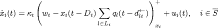
where hi > 0, τi > 0 are some parameters of the TDFC to be designed.
Define
![]()
where ![]() is the unique equilibrium point of the system. Linearizing the system (5.149)–(5.150) with (5.148) about the equilibrium yields
is the unique equilibrium point of the system. Linearizing the system (5.149)–(5.150) with (5.148) about the equilibrium yields
where p′ l is the derivative of pl evaluated at ![]() , i.e.,
, i.e., ![]() . Assuming the initial state is zero, we take the Laplace transform and obtain
. Assuming the initial state is zero, we take the Laplace transform and obtain
where ![]() is the Laplace transform of
is the Laplace transform of ![]() . Define the following matrices:
. Define the following matrices:
(5.153) ![]()
(5.154) ![]()
(5.155) ![]()
(5.156) ![]()
(5.157) ![]()
Then, (5.152) can be written in the matrix form as
where ![]() .
.
For s = 0, we have
![]()
where R = Rf(0) is the routing matrix. Because ![]() are all positive in the primal algorithm, −M(0)diag{e−0×Di} is a negatively definite matrix. By Lemma 5.25, we find that system (5.151) does not have the odd number limitation. This encourages us to apply the TDFC to the primal algorithm.
are all positive in the primal algorithm, −M(0)diag{e−0×Di} is a negatively definite matrix. By Lemma 5.25, we find that system (5.151) does not have the odd number limitation. This encourages us to apply the TDFC to the primal algorithm.
Theorem 5.26. There exist hi and τi for ![]() such that the primal algorithm (5.149)–(5.150) with TDFC given by (5.148) is locally stable at the equilibrium point.
such that the primal algorithm (5.149)–(5.150) with TDFC given by (5.148) is locally stable at the equilibrium point.
This theorem suggests that when the TDFC method is combined with the primal algorithm proposed by Kelly, Maulloo and Tan (1998), for any round-trip delays the network can be stabilized at the prescribed equilibrium point which is unknown for each source node, and thus the stability is much enhanced. In Chapter 1 we have shown some numerical examples of applying TDFC to eliminating oscillations in congestion control system.
Before giving a complete proof of Theorem 5.26, we need to make some preparation. First, let us prove the following lemma.
Lemma 5.27. The quasi-polynomial
![]()
has no RHP roots for any h > 0 and τ > 0.
Proof. Let
![]()
Then, f(s) has no RHP roots if and only if F(s) has no RHP zeros. By Nyquist the stability criterion, F(s) has no RHP zeros if and only if the Nyquist plot of
![]()
does not enclose the point (− 1, j0) in the complex plane. So,
It is easy to get
![]()
Now, let
![]()
then we have τω = 2kπ(k ≠ 0) which implies
![]()
Therefore, for any h > 0 the Nyquist plot of G(jω) intersects the real axis of the complex plane only at the origin.
Now, let us investigate the role of TDFC for stabilization of a first-order time-delayed system. The following lemma shows that an analog of the odd number limitation holds for the first-order time-delayed system.
Lemma 5.28. The first-order time-delayed system
with any delay constant D > 0 can be asymptotically stabilized by TDFC (5.148) if and only if a > 0.
Proof. (Necessity) Since system (5.160) is a special case of system (5.146) with n = 1 and nd = 1, the necessity part is provided by Lemma 5.25.
(Sufficiency) The closed-loop form of system (5.160) with TDFC (5.148) is given by
(5.161) ![]()
where a > 0, D > 0. The characteristic equation of the above system is
We will prove that there exists h and τ such that all the roots of this equation lie inside the LHP.
Let
![]()
Then, the characteristic equation can be written as 1 + F1(s) = 0, s ≠ 0. We adopt the Nyquist stability criterion to continue the proof. Consider the frequency property function of F1(s) given by
(5.163) 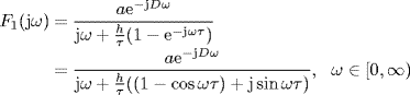
As shown by Lemma 5.27, F1(s) has no RPH poles. So, by the Nyquist stability criterion, all the roots of (5.162) lie inside the LHP if and only if the Nyquist plot of F1(jω) does not enclose the point (− 1, j0) in the complex plane. Let ωc1 denote the frequency at which F1(jω) crosses the real axis for the first time. It suffices to prove that |F1(jω)| < 1 for ω ![]() [ωc1, ∞).
[ωc1, ∞).
We choose τ < D. Thus,
![]()
for ![]() , where arg (·) denotes the phase. By noticing that
, where arg (·) denotes the phase. By noticing that
![]()
and
![]()
we know that
![]()
from the continuous property of arg (F1(jω)). So we have
![]()
where
Therefore,
(5.165) 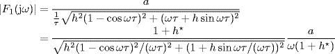
(5.166) ![]()
![]()
Choose h such that ![]() . There exists a positive constant q1 < π/2 such that
. There exists a positive constant q1 < π/2 such that ![]() for q
for q ![]() (0, q1]. Thus, F2(ωτ) < 1 for ωτ
(0, q1]. Thus, F2(ωτ) < 1 for ωτ ![]() (0, q1], i.e. ω
(0, q1], i.e. ω ![]() (0, q1/τ]. Obviously, there exists a positive constant ξ < D such that ωc1 < q1/τ, and hence,
(0, q1/τ]. Obviously, there exists a positive constant ξ < D such that ωc1 < q1/τ, and hence, ![]() with τ
with τ ![]() (0, ξ).
(0, ξ).
In the following, we prove that by choosing τ we can ensure |F1(jω)| < 1 for ω ![]() (q1/τ, ∞) with h > |h*|. It is equivalent to ensure that G(ω) > a2 for ω
(q1/τ, ∞) with h > |h*|. It is equivalent to ensure that G(ω) > a2 for ω ![]() (q1/τ, ∞) with
(q1/τ, ∞) with
For h > |h*|, where h* is given by (5.164), we consider the following two cases with different values of h.
Case 1: h ≤ 1.5π.
From (5.167) it is easy to see
![]()
for ωτ ![]() [q1, 2π − q1], and hence, there exists a positive constant ξ11 such that
[q1, 2π − q1], and hence, there exists a positive constant ξ11 such that
![]()
for τ ![]() (0, ξ11) and
(0, ξ11) and
![]()
for ωτ ![]() (2π − q1, ∞). Thus, there also exists a positive constant ξ12 such that
(2π − q1, ∞). Thus, there also exists a positive constant ξ12 such that
![]()
for τ ![]() (0, ξ12). Therefore, by choosing
(0, ξ12). Therefore, by choosing
![]()
we can ensure G(ω) > a2, i.e.,
![]()
for ω ![]() (q1/τ, ∞).
(q1/τ, ∞).
Case 2: h > 1.5π.
Define
![]()
Obviously, for g > 0, the equation χ(g) = 0 has solutions when h > 1.5π. Take these solutions of χ(g) = 0 as a sequence {g(n), n = 1, . . . } with certain length. Rank the elements of {g(n), n = 1, . . . } increasingly. Then, we get
![]()
To consider the minimums of G(ω), we compute the derivative of G(ω) with respect to ω as follows
(5.168) 
Obviously,
![]()
and
![]()
Thus, G(ω) may have a minimum at ![]() , and
, and
![]()
Therefore, we can choose a positive constant ξ21 to make ![]() with τ
with τ ![]() (0, ξ21). Then, f(ωτ) > 0 for
(0, ξ21). Then, f(ωτ) > 0 for ![]() . Hence, G(ω) has a minimum at
. Hence, G(ω) has a minimum at ![]() , and
, and
![]()
Therefore, there also exists a positive constant ξ22 such that ![]() with τ
with τ ![]() (0, ξ22). Similarly, when ωτ > 2π, we can also ensure that G(ω) > a2 at the minimum of G(ω) by choosing τ. Therefore, we can choose a positive constant ξ2 finally to make G(ω) > a2, i.e. |F1(jω)| < 1 for ω
(0, ξ22). Similarly, when ωτ > 2π, we can also ensure that G(ω) > a2 at the minimum of G(ω) by choosing τ. Therefore, we can choose a positive constant ξ2 finally to make G(ω) > a2, i.e. |F1(jω)| < 1 for ω ![]() (q1/τ, ∞) with τ
(q1/τ, ∞) with τ ![]() (0, ξ2).
(0, ξ2).
As discussed above, there exist K = h/τ with h > |h*|, and τ ![]() (0, min (ξ, ξ1)) for case 1 or τ
(0, min (ξ, ξ1)) for case 1 or τ ![]() (0, min (ξ, ξ2)) for case 2 such that system (5.160) is stable. Lemma 5.28 is thus proved.
(0, min (ξ, ξ2)) for case 2 such that system (5.160) is stable. Lemma 5.28 is thus proved.
Now, we provide the proof of Theorem 5.26 as follows.
Proof of Theorem 5.26
From (5.159) we get the characteristic equation of the closed-loop system with TDFC as follows:
![]()
Since the equation
![]()
has no RHP roots for any ![]() according to Lemma 5.27, from the general Nyquist stability criterion (Theorem 2.20) we know that the system (5.159) is asymptotically stable, if and only if the eigenloci of
according to Lemma 5.27, from the general Nyquist stability criterion (Theorem 2.20) we know that the system (5.159) is asymptotically stable, if and only if the eigenloci of ![]() , i.e.
, i.e.
![]()
do not enclose the point (− 1, j0) for ω ![]() [0, ∞). Denote
[0, ∞). Denote
where
and
Then, we have
Hence, from Lemma 2.34 it follows that
Using Corollary 2.31 of Gershgorin's disc lemma and (5.169)–(5.171) as well, we have
Define
![]()
and
![]()
Then, we just need to prove that there exist hi and τi such that
![]()
for all ω ![]() (0, ∞).
(0, ∞).
Choose hi such that ![]() . There always exists a positive constant qi < π/2 such that
. There always exists a positive constant qi < π/2 such that ![]() for q
for q ![]() (0, qi], and
(0, qi], and
From the proof of Lemma 5.28 we know that F2i(jω) crosses the real axis at ![]() for the first time with 0 < τi < Di. Thus, there always exist
for the first time with 0 < τi < Di. Thus, there always exist ![]() such that
such that ![]() with τi
with τi ![]() (0, ςi1).
(0, ςi1).
When ![]() , we have
, we have
from (5.172) and the fact that
According to the proof of Theorem 3.10, all the Nyquist plots of ![]() have the same shape, and cross the real axis for the first time at (− 1, j0). Let r(− 1, j0) denote the tangent line to
have the same shape, and cross the real axis for the first time at (− 1, j0). Let r(− 1, j0) denote the tangent line to ![]() at (− 1, j0). Then, by Lemma 3.9, the complex plane is divided into two parts by r(− 1, j0), and the Nyquist plot of F1i(jω) is in one side of r(− 1, j0) (see Figure 5.18). Because of (5.173) and (5.174) as well as the fact that
at (− 1, j0). Then, by Lemma 3.9, the complex plane is divided into two parts by r(− 1, j0), and the Nyquist plot of F1i(jω) is in one side of r(− 1, j0) (see Figure 5.18). Because of (5.173) and (5.174) as well as the fact that ![]() decreases as the phase arg (F1i(jω)) decreases, |F2i(jω)| is less than |F1i(jω)| at the same phase. Therefore, for
decreases as the phase arg (F1i(jω)) decreases, |F2i(jω)| is less than |F1i(jω)| at the same phase. Therefore, for ![]() , the Nyquist plot of F2i(jω) is on the same side of r(− 1, j0) as that of F1i(jω), and it doesn't have any intersection with r(− 1, j0) (Figure 5.18). Therefore,
, the Nyquist plot of F2i(jω) is on the same side of r(− 1, j0) as that of F1i(jω), and it doesn't have any intersection with r(− 1, j0) (Figure 5.18). Therefore,
![]()
for all ![]() , 0 < κ ≤ 1. By Lemma 2.34, we come to the conclusion that
, 0 < κ ≤ 1. By Lemma 2.34, we come to the conclusion that
![]()
for all ![]() with τi
with τi ![]() (0, ςi1).
(0, ςi1).
Figure 5.18 Nyquist plots.
When ![]() , analogous to the proof of Lemma 5.28, there always exist
, analogous to the proof of Lemma 5.28, there always exist ![]() to make |F2i(jω)| < 1 for
to make |F2i(jω)| < 1 for ![]() with τi
with τi ![]() (0, ςi2). (For illustration we show the general shape of the Nyquist plot of F2i(jω), i = 1, 2, 3 for
(0, ςi2). (For illustration we show the general shape of the Nyquist plot of F2i(jω), i = 1, 2, 3 for ![]() in Figure 5.19.) Hence,
in Figure 5.19.) Hence,
![]()
for all ![]() , 0 < κ ≤ 1. By Lemma 2.34, we come to the conclusion that
, 0 < κ ≤ 1. By Lemma 2.34, we come to the conclusion that
![]()
for all ![]() with τi
with τi ![]() (0, ςi2).
(0, ςi2).
Figure 5.19 High frequency property of Nyquist plots.
From the above discussion, there exist Hi = hi/τi with
![]()
and
![]()
such that
![]()
for ω ![]() (− ∞, ∞). Therefore, the system (5.159) is stable. Theorem 5.26 is proved.
(− ∞, ∞). Therefore, the system (5.159) is stable. Theorem 5.26 is proved.
5.5.3 Design of TDFC with Commensurate Self-Delays
Theorem 5.26 proves the existence of TDFC that stabilizes Kelly's primal algorithm with any round-trip delays. However, it does not provide an explicit procedure for the design of the control parameters (self-delays τi and gains hi) of TDFC. In this subsection we present a design scheme by considering the case when self-delays and round-trip delays are commensurate. Note that delays τ1, . . . , τm are said to be commensurate if τi/τj is rational for all ![]() (Gu, Kharitonov and Chen (2003). In this case we can always find a τ such that τi = kiτ for all
(Gu, Kharitonov and Chen (2003). In this case we can always find a τ such that τi = kiτ for all ![]() , where ki are integers.
, where ki are integers.
Let us first introduce some preliminary lemmas.
Lemma 5.29 For any positive integer k, the following equalities hold:
Proof. The lemma can be easily proved by making induction on k. The details are left to the reader as an exercise.
Exercises 5.30 Prove Lemma 5.29.
By Lemma 5.29 we can always expand cos kx as a polynomial of cos x, i.e.,
Lemma 5.31 For any positive integer k and ![]() such that sin x ≠ 0, the following inequality holds
such that sin x ≠ 0, the following inequality holds
![]()
moreover, the equality holds if and only if k = 1.
Proof. Obviously, the equality holds if k = 1. Therefore, the rest task of the proof is to prove that
![]()
for any integer k > 1.
Since the function ![]() is π-periodic and symmetric about x = − π/2, i.e.,
is π-periodic and symmetric about x = − π/2, i.e.,
![]()
we just need to show the equality is true for x ![]() (0, π/2].
(0, π/2].
When ![]() , we have sin x > 0, sin kx > 0. Let f(x) = sin kx − k sin x. Then, in the given interval we have f′ (x) = k(cos kx − cos x) < 0 for k > 1. Therefore, f(x) < f(0) = 0.
, we have sin x > 0, sin kx > 0. Let f(x) = sin kx − k sin x. Then, in the given interval we have f′ (x) = k(cos kx − cos x) < 0 for k > 1. Therefore, f(x) < f(0) = 0.
When ![]() , we have
, we have
![]()
At the last step of the above derivation we used the well-known inequality ![]() for any x
for any x ![]() (0, 1].
(0, 1].
Lemma 5.32 Suppose that ![]() , where n is any positive integer. Then,
, where n is any positive integer. Then,
holds for all ω ≠ 0, if
where e1, . . . , en are coefficients of ![]() defined by (5.175).
defined by (5.175).
Proof. For convenience we denote ξ = 1/n and
![]()
Due to the symmetry of g(jω) we just need to prove (5.176) for ω > 0. Since
![]()
Re(g(jω)) > − 1 if and only if
Denote x = Dω. Then, (5.178) holds for all ω ≠ 0 and ![]() if and only if
if and only if
(5.179) ![]()
for x ≠ 0 and ![]() .
.
We first consider the case when
Straightforward calculation yields
(5.181) 
where k = 2n − 1. By Lemma 5.31 and (5.177), we know that
So, (5.180) holds if and only if
![]()
This implies that sin ξx = sin x = 0, and 2x ![]() sin ξx − ax sin x = 0, which further implies that f(x, D) = x2 in this case. Thus, f(x, D) > 0 for all x ≠ 0 and
sin ξx − ax sin x = 0, which further implies that f(x, D) = x2 in this case. Thus, f(x, D) > 0 for all x ≠ 0 and ![]() .
.
Now, we consider the case when
(5.184) ![]()
By (5.182) and (5.183), we have ![]() and
and
![]()
So, in this case f(x, D) can be considered as a quadratic polynomial of D with a positive coefficient of the second order term. Then, f(x, D) < 0 if and only if the discriminant
where α, β, ζ are the coefficients of the quadratic polynomial f(x, D). Straightforward calculation shows that
![]()
So, (5.185) holds if
![]()
By using Lemma 5.29 we have
where ![]() . Obviously, −1 ≤ z < 1 because
. Obviously, −1 ≤ z < 1 because ![]() . It follows from (5.177) that
. It follows from (5.177) that
which implies that
![]()
When ![]() , we have cos x = 1, and thus, u(1) = 2
, we have cos x = 1, and thus, u(1) = 2 ![]() − a. So, u(z) < u(1) = 2
− a. So, u(z) < u(1) = 2 ![]() − a for all −1 ≤ z < 1. Therefore, (5.185) is indeed true. The proof of the lemma is thus completed.
− a for all −1 ≤ z < 1. Therefore, (5.185) is indeed true. The proof of the lemma is thus completed.
Now, we can present the following result which provides an explicit procedure for the design of the parameters of the TDFC.
Theorem 5.33 Consider the primal algorithm (5.149)–(5.150) with TDFC given by
(5.187) ![]()
Take
(5.188) ![]()
where ![]() are any positive integers. Then, the closed-loop system is locally stable at the equilibrium point, if
are any positive integers. Then, the closed-loop system is locally stable at the equilibrium point, if
![]()
where
and ![]() are coefficients of
are coefficients of ![]() defined by (5.175).
defined by (5.175).
Proof. Similar to the proof of Theorem 5.26, we get the characteristic equation of the linearized closed-loop system as
![]()
Since the equation
![]()
has no RHP roots for any ![]() according to Lemma 5.27, from the general Nyquist stability criterion (Theorem 2.20) we know that the system (5.159) is asymptotically stable, if and only if the eigenloci of
according to Lemma 5.27, from the general Nyquist stability criterion (Theorem 2.20) we know that the system (5.159) is asymptotically stable, if and only if the eigenloci of ![]() , i.e.
, i.e.
![]()
do not enclose the point (− 1, j0) for ω ![]() [0, ∞), where M(s) is defined by (5.158).
[0, ∞), where M(s) is defined by (5.158).
Denote
Then, we have
Hence, from Lemma 2.34 it follows that
Using Corollary 2.31 of Gershgorin's disc lemma, (5.190) and (5.189), we have ![]() . By Lemma 5.32 we know
. By Lemma 5.32 we know
![]()
and hence,
![]()
Theorem 5.33 is thus proved.
Example 5.34 Design of TDFC for stabilizing the primal algorithm with diverse round-trip delays.
Consider a network with three links shared by four sources, which is illustrated by Figure 5.20. Obviously, the routing matrix of this network is
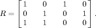
The congestion control algorithm is given by
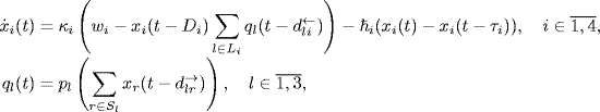
where pl(y) = 1 − (1 − y)ey, ![]() . Let
. Let ![]() and
and ![]() . Then, we get the equilibrium as
. Then, we get the equilibrium as ![]() (Mbps),
(Mbps), ![]()
Figure 5.20 A network controlled by TDFC.
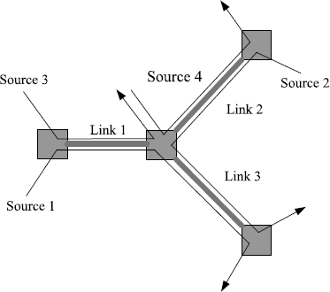
Take D1 = D4 = 500s, D2 = D3 = 100s; and κ1 = 0.0611, κ2 = 0.3053, κ3 = 0.6107, κ4 = 0.1221. Then, oscillation is observed in the network. Now, we take two sets of parameters of TDFC as τi = Di, ![]() i = ai and τi = Di/2,
i = ai and τi = Di/2, ![]() i = 3ai, respectively, where ai is determined by (5.189). The TDFC is put on after t ≥ 104s. The simulation results for the two case are shown in Figure 5.21 and Figure 5.22, respectively. We see that in both cases the network is stabilized by TDFC. Now, we take τ = kDi, where k is set as 0.1, 0.2, 0.3, . . . , 1.4, respectively; and
i = 3ai, respectively, where ai is determined by (5.189). The TDFC is put on after t ≥ 104s. The simulation results for the two case are shown in Figure 5.21 and Figure 5.22, respectively. We see that in both cases the network is stabilized by TDFC. Now, we take τ = kDi, where k is set as 0.1, 0.2, 0.3, . . . , 1.4, respectively; and ![]() i = ai. Then, we have found the network is also stabilized. The experiments tell us that the TDFC designed by Theorem 5.33 is robust against non-commensurate self-delays.
i = ai. Then, we have found the network is also stabilized. The experiments tell us that the TDFC designed by Theorem 5.33 is robust against non-commensurate self-delays.
Figure 5.21 Source rates under TDFC.
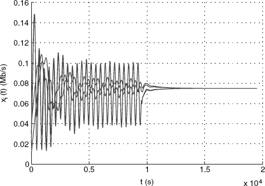
Figure 5.22 Sources rate under TDFC.
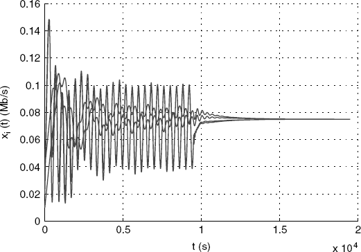
5.6 Notes and References
5.6.1 Stability of Congestion Control with Propagation Delays
As one of most important topics in congestion control, the stability issue has drawn much attention (Kelly 2003; Liu et al. 2003). The primal algorithm and the dual algorithm have been proved globally asymptotically stable in the absence of delay (Kelly, Maulloo and Tan 1998; Low and Lapsley 1999; Paganini 2002). Johari and Tan (2001) investigated the primal algorithm with propagation delays. They gave a nice decomposition of the transfer function matrix of the feedback congestion control system into a product of a diagonal and a Hermitian matrix, and used this to derive some sufficient conditions for the local stability of networks with the same round-trip delays for different TCP connections. For a more general case of networks with diverse round-trip delays, they proposed a conjecture (Conjecture 5.1) on the local stability of the algorithm. A weaker version of the continuous-time analogue of the conjecture (Conjecture 5.3) was proved by Massoulie (2002). To prove Conjecture 5.3 Vinnicombe (2000) proposed an elegant lemma (Lemma 2.34) which relates the eigenloci of the product of a Hermitian matrix and a diagonal matrix to the product of the spectral radius of the Hermitian matrix and the convex hull of the entries of the diagonal matrix. Using this lemma and the generalized Nyquist criterion (Desoer and Wang (1980), Vinnicombe illustrated the correctness of Conjecture 5.3. Tian and Yang (2004b) proved a more general stability criterion (Theorem 5.4) which includes Conjecture 5.3 as a special case. However, the scheme of Vinnicombe (2000) does not show the correctness of the original conjecture of Johari and Tan (Conjecture 5.1). Using the clockwise property of Nyquist plot of the time-delayed Tian and Yang (2004a (2004a) gave a rigorous proof of the Conjecture 5.1 via proving a more general stability criterion (Theorem 5.2). Theorem 5.2 preserves the elegance of Conjecture 5.1 being decentralized and locally implemented and enlarges the stability region of control gains and admissible communication delays. Tian (2005) and Tian and Chen (2006) analyzed the REM algorithm and the primal-dual algorithm respectively, and found that the clockwise property plus some other nice geometric properties of the dynamics of congestion control algorithms in a certain frequency interval determines the the scalability of these congestion control algorithms.
5.6.2 Time-Delayed Feedback Control
The original TDFC proposed by Pyragas (1992) was extended to multiple-delay systems (Socolar et al. (1994), observer-based version (Tian and Chen 2001) and a predictor-based version (Nakajima 2002). Ushio (1996) first studied the stability of the TDFC for discrete-time systems. The multiple-delay TDFC (Konishi, Ishii and Kokame 1999), observer-based TDFC (Konishi and Kokame 1998) and the predictor-based TDFC (Ushio and Yamamoto 1999) for discrete-time systems were also proposed in parallel with continuous-time systems. Finally, the TDFC was even extended to systems described by partial differential equations (Bleich and Socolar 1996; Harrington and Socolar 2001) and hybrid systems (Tian, Yu and Chua 2004).
In stability analysis for discrete-time systems under TDFC, Ushio (1996) proved that the TDFC has an inherent limitation, known as “odd number limitation”. Ushio and Yamamoto (1998) gave a linear matrix inequality condition for designing the gain matrix of TDFC for a discrete-time system. Ushio and Yamamoto (1998) also showed that the odd number limitation can be overcome by using a nonlinear time-delayed feedback control method. Konishi and Kokame (1998), Ushio and Yamamoto (1999), and Yamamoto, Hino and Ushio (2001) then showed that the odd number limitation for discrete-time systems can also be overcome by other methods such as observer-based TDFC, predictor-based TDFC and dynamical TDFC.
For continuous-time systems, Nakajima (1997) proved that the odd number limitation holds for general higher-dimensional continuous-time systems under TDFC. Nakajima and Ueda (1998) further showed that the odd number limitation also holds for TDFC with multiple-delays. Tian and Chen (2001) proved that the odd number limitation exists in the case of observer-based dynamical output TDFC. Lemma 5.25 which was first given by Liu and Tian (2008) shows that the odd number limitation exists in systems with multiple delays.
However, the odd number limitation just gives a necessary condition of the stabilizability under TDFC. Kokame et al. (2001) proved that for a continuous-time system with single input, this condition is also sufficient for the existence of a stabilizing TDFC. Lemma 5.28 extends this result to scalar time-delayed systems. But this conclusion does not apply to discrete-time systems. Zhu and Tian (2005) found a new upper bound and gives a necessary and sufficient condition of the existence of a stabilizing TDFC for discrete-time systems with single input. Tian and Zhu (2004) gives a full characterization on stabilizability single input discrete-time systems under extended TDFC.
Chen, Wang and Han (2004) and Jiang, Wang and Xi (2004) used TDFC to adjust some parameters of the RED algorithm, an AQM algorithm in the Internet congestion control (Floyd and Jacobson 1993). Liu and Tian (2008) introduced the TDFC as a stabilizer in distributed congestion control systems. Theorem 5.26 which is due to Liu and Tian (2008) shows that the primal algorithm with any diverse round-trip delays can always be stabilized by distributed TDFC. Theorem 5.33 is a new result which provides an explicit design procedure of TDFC for distributed time-delayed systems.
Athuraliya S, Low SH and Yin Q (2001). REM: Active Queue Management. IEEE Network, 15, 48–53.
Basso M, Genesio R, and Tesi A (1997). Stabilizing periodic orbits of forced systems via generalized Pyragas controllers. IEEE Transactions on Circuits and Systems–I, 44(10), 1023–1027.
Bleich ME and Socolar JES (1996). Controlling spatiotemporal dynamics with time-delay feedback. Physics Review E, 54, R17–R20.
Chen L, Wang X and Han Z (2004). Control chaos in internet congestion control model. Chaos, Solitons & Fractals, 21, 81–91.
Desoer CA and Wang Y-T (1980). On the generalized Nyquist Stability Criterion. IEEE Transactions on Automatic Control, 25(2), 187–196.
Floyd S and Jacobson V (1993). Random early detection gateways for congestion avoidance. IEEE/ACM Transactions on Networking, 1, 397–413.
Gu K, Kharitonov VL and Chen J (2003). Stability of Time-delayed Systems. Birkhäuser, Boston.
Harrington I and Socolar JES (2001). Limitation on stabilizing plane waves via time-delayed feedback. Physics Review E, 64(5), 056206(6).
Hino T, Yamamoto S and Ushio T (2002). Stabilization of unstable periodic orbits of chaotic discrete-time systems using prediction-based feedback control. International Journal Bifurcation and Chaos, 12(2), 439–446.
Jiang K, Wang X and Xi Y (2004). A robust RED algorithm based on time-delayed feedback control. Proceeding of the 5th Asian Control Conference 2, 708–713.
Johari R and Tan D (2001). End to end congestion control for the internet: delays and stability. IEEE/ACM Transactions on Networking, 9, 818–832.
Just W, Bernard T, Ostheimer M, Reibold E and Benner H (1997). Mechanism of time-delayed feedback control. Physics Review Letters, 78(2), 203–206.
Just W, Reckwerth D, Mockel J, Reibold E and Benner H (1998). Delayed feedback control of periodic orbits in autonomous systems. Physics Review Letters, 81(3), 562–565.
Kelly FP, Maulloo A and Tan D (1998). Rate control for communication networks: shadow prices proportional fairness and stability. Journal of the Operational Research Society, 49, 237–252.
Kelly FP (2003). Fairness and stability of end-to-end congestion control. European Journal of Control, 9, 149–165.
Kokame H, Hirata K, Konishi K and Mori T (2001). Difference feedback can stabilize uncertain steady states. IEEE Transactions on Automatic Control, 46, 1908–1913.
Konishi K and Kokame H (1998). Obsever-based delayed-feedback control for discrete-time chaotic systems. Physics Letters A, 248(5-6), 359–368.
Konishi K, Ishii M and Kokame H (1999). Stability of extended delayed-feedback control for discrete-time chaotic system. IEEE Transactions on Circuits and Systems–I, 46(10), 1285–1288.
Li C, Chen G, Liao X and Yu J (2004). Hopf bifurcation in an Internet congestion control model. Chaos, Solitons & Fractals 6, 853–62.
Liu C-L and Tian Y-P (2008). Eliminating oscillations in the Internet by time-delayed feedback control. Chaos, Solitons and Fractals, 35, 878–887
Liu S, Ba![]() ar T and Srikant R (2003). Controlling the Internet: A survey and some new results. Proceedings of IEEE Conference on Decision and Control, Maui, Hawaii.
ar T and Srikant R (2003). Controlling the Internet: A survey and some new results. Proceedings of IEEE Conference on Decision and Control, Maui, Hawaii.
Low SH and Lapsley DE (1999). Optimization flow control–I: basic algorithm and convergence. IEEE/ACM Transactions on Networking, 7, 861–874.
Massoulie L (2002). Stability of distributed congestion control with heterogeneous feedback delays. IEEE Transactions on Automatic Control, 47, 895–902.
Moon FC (1987). Chaotic vibrations. John Wiley, New York.
Nakajima H (1997). On analytical properties of delayed feedback control of chaos. Physics Letters A, 232, 207–210.
Nakajima H and Ueda Y (1998). Limitation of generalized delayed feedback control. Physica D, 111, 143–150.
Nakajima H (2002). Delayed feedback control with state predictor for continuous-time chaotic system. International Journal of Bifurcation and Chaos, 12(5), 1067–1077.
Ott E, Simmendinger C and Hess O (1996). Controlling delayed-induced chaotic behavior of a semiconductor laser with optical feedback. Physics Letters A, 216, 97–105.
Paganini F (2002). A global stability result in network flow control. Systems & Control Letters, 40, 165–172.
Parmananda P, Madrigal R and de Ciencias MRF (1999). Stabilization of unstable steady states and periodic orbits in an electrochemical system using delayed-feedback control. Physics Review E, 59(5), 5266–5271.
Peitgen H-O, Jürgens H and Saupe D (1993). Chaos and Fractal, new frontiers of science. Springer-Verlag.
Pyragas K (1992). Continuous control of chaos by self-controlling feedback. Physics Letters A, 170, 421–428.
Schuster H (1984). Deterministic Chaos. Physik Verlag, Weinheim.
Socolar JES, Sukow DW and Gauthier DJ (1994). Stabilizing unstable periodic orbits in fast dynamics, Physics Review E, 50(5), 3245–3248.
Tian Y-P and Chen G (2001). A separation principle for dynamical delayed output feedback control of chaos. Physics Letters A 284, 31–42.
Tian Y-P, Yu X and Chua LO (2004). Time-delayed impulsive control of hybrid chaotic systems. International Journal of Bifurcation and Chaos, 14(3), 1091–1104.
Tian Y-P and Yang H-Y (2004a). Stability of the Internet congestion control with diverse delays. Automatica, 40, 1533–1541.
Tian Y-P and Yang H-Y (2004b). Stability of distributed congestion control with diverse communication delays. Proceedings of the World Congress on Intelligent Control and Automation 2, 1438–1442.
Tian Y-P and Zhu J (2004). Full characterization on limitation of generalized delayed feedback control for discrete-time systems. Physica D 198, 248–257.
Tian Y-P (2005). Stability analysis and design of the second-order congestion control for networks with heterogeneous delays. IEEE/ACM Transactions on Networking, 13, 1082–1093.
Tian Y-P and Chen G (2006). Stability of the primal-dual algorithm for congestion control. International Journal of Control, 79, 662–676.
Ushio T (1996). Limitation of delayed feedback control in nonlinear discrete-time systems. IEEE Transactions on Circuits and Systems–I, 43, 815–816.
Ushio T and Yamamoto S (1998). Delayed feedback with nonlinear estimation in chaotic discrete-time system. Physics Letters A, 247, 112–118.
Ushio T and Yamamoto S (1999). Prediction-based control of chaos. Physics Letters A, 264, 30–35.
Vinnicombe G (2000). On the stability of end-to-end congestion control for the Internet. Technical report CUED/F-INFENG/TR., No.398, 2000.
Wiggins S (1988). Global Bifurcations and Chaos. Analytical Methods, Springer-Verlag.
Yamamoto S, Hino T and Ushio T (2001). Dynamical delayed feedback controllers for chaotic discrete-time systems. IEEE Transactions on Circuits and Systems–I, 48(6), 785–789.
Yamamoto S and Ushio T (2003). Odd number limitation in delayed feedback control. Chaos Control: Theory and Application, edited by G. Chen and X. Yu, Lecture Notes in Control and Information Sciences, 292, 71–87, Springer, Berlin.
Yang H-Y and Tian Y-P (2005). Hopf bifurcation in REM algorithm with communication delay. Chaos, Solitons & Fractals, 25, 1093–1105.
Yin Q and Low SH (2001). Convergence of REM flow control at a single link. IEEE Communication Letters, 5, 119–121.
Yin Q and Low SH (2002). On stability of REM algorithm with uniform delay. GLOBECOM ’02, IEEE, 3, 2649–2653.
Zhu J and Tian Y-P (2005). Necessary and sufficient conditions for stabilizability of discrete-time systems via delayed feedback control. Physics Letters A 343, 95–107.