
Chapter 6
Consensus in Homogeneous Multi-Agent Systems
Like seeks to like, and (birds) of the same note respond to one another –this is a rule of Heaven.
—Zhuang Zi (368–286 BC), ‘The Old Fisherman'
Cooperation is a central topic in the design of a distributed control system. One of the most convenient and efficient approaches to undertaking a cooperative task for the agents of a distributed control system is to achieve some agreement (consensus). This chapter introduces basic notions in consensus problems, such as consensus protocol, the existence of consensus solutions and consentability. A unified approach to treating the consensus problem as a stability problem is presented. The consensus problem for systems with homogeneous agents of the first order, second order and nth order is investigated.
6.1 Introduction to Consensus Problem
In this section we introduction some basic notions in consensus problems by considering a simple multi-agent system: a system with integrator agents over an ideal network, i.e., a network without communication delays.
6.1.1 Integrator Agent System
Consider a multi-agent system with a fixed topology digraph G = (V, E, A). Each agent can be considered as a node in the digraph, and an information flow between two agents can be regarded as a directed path between two nodes. Each dynamic agent is described by
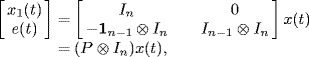
where ![]() and
and ![]() , and
, and ![]() . The control ui adopts the following consensus protocol
. The control ui adopts the following consensus protocol
where γ > 0 is the control gain.
We say a consensus solution (or consensus in short) is asymptotically achieved in the system if
(6.3) ![]()
6.1.2 Existence of Consensus Solution
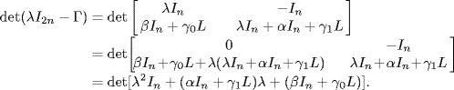
Let x = [x1, x2, . . . , xn]T. With the control protocol (6.2), the closed-loop system can be written in the matrix form as
where L = {lij} is the Laplacian matrix of digraph G.
By Theorem 1.9, LC = 0 for any C ![]() span(1n). This implies that the system (6.1) with protocol (6.2) (namely, system (6.4)) indeed contains a consensus solution x1(t) = x2(t) =
span(1n). This implies that the system (6.1) with protocol (6.2) (namely, system (6.4)) indeed contains a consensus solution x1(t) = x2(t) = ![]() = xn(t) = c, where
= xn(t) = c, where ![]() is a constant determined by the initial condition of the system. Actually, all the consensus solutions
is a constant determined by the initial condition of the system. Actually, all the consensus solutions ![]() form a continuum of equilibria of the system, denoted by Xe.
form a continuum of equilibria of the system, denoted by Xe.
6.1.3 Consensus as a Stability Problem
To check if the system asymptotically achieves a consensus solution in Xe, let us introduce the error variables
(6.5) ![]()
Denote e = [e1, . . . , en−1]T. Then, we get
where
Obviously, system (6.4) reaches the consensus asymptotically if and only if system (6.6) is asymptotically stable.
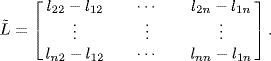
Proposition 6.1. Let the eigenvalues of L be denoted as 0, μ2, . . . , μn. Then, the eigenvalues of ![]() defined by (6.7) are μ2, . . . , μn.
defined by (6.7) are μ2, . . . , μn.
Proof. By choosing a nonsingular transformation matrix
we have ![]() , where ϕ = [l12, l13, . . . , l1n]. This implies that the eigenvalues of
, where ϕ = [l12, l13, . . . , l1n]. This implies that the eigenvalues of ![]() are exactly the remaining n − 1 eigenvalues of L excluding zero.
are exactly the remaining n − 1 eigenvalues of L excluding zero. ![]()
Therefore, by Theorem 1.9, all the eigenvalues of ![]() have positive real parts if and only if the digraph G contains a globally reachable node. Thus, the following theorem is obtained.
have positive real parts if and only if the digraph G contains a globally reachable node. Thus, the following theorem is obtained.
Theorem 6.2 System (6.1) with protocol (6.2) reaches a consensus solution asymptotically if and only if the interconnection topology digraph G contains a globally reachable node.
6.1.4 Discrete-Time Systems
Consider the discrete-time system
with consensus protocol
In a similar way to that shown in Section 6.1.3, the consensus problem for the discrete-time system can be converted to the stability problem for the following system
![]()
Then, one can easily obtain the consensus condition for the system which is summarized in the following theorem.
Theorem 6.3 System (6.9) with protocol (6.10) reaches a consensus solution asymptotically if and only if the interconnection topology digraph G(V, E, A) has a globally reachable node and the following condition holds:
where μi's are the eigenvalues of the Laplacian matrix L(G) except for zero.
Remark. By Corollary 2.31 of Gershgorin's disc lemma, it is easy to get a sufficient but scalable condition for (6.11) as
(6.12) ![]()
6.1.5 Consentability
For a multi-agent system, if there exists a consensus protocol such that a consensus can be reached asymptotically, then we say the system is consentable. Theorem 6.2 (Theorem 6.3) tells us that there always exists a control gain γ such that system (6.1) with protocol (6.4) (system (6.9) with protocol (6.10)) can reach a consensus solution provided the interconnection topology digraph G contains a globally reachable node. So, for the system with integrator agents over ideal networks the connectivity of the graph serves as the sole condition of consentability.
Exercises 6.4 Prove that Theorem 6.2 and Theorem 6.3 are true for the case when the states in (6.1) and (6.9) are p-dimensional vectors, i.e., ![]() .
.
(Hint: Reformulate the consensus problem as a stability problem, i.e.,
![]()
for the continuous-time system, and
![]()
for the discrete-time system, where ⊗ denotes the Kronecker product, ![]() , and
, and ![]() .)
.)
6.2 Second-Order Agent System
6.2.1 Consensus and Stability
Now, we consider dynamic agents with second-order dynamics
where ![]() and
and ![]() are the states (for many physical systems they represent the position and velocity);
are the states (for many physical systems they represent the position and velocity); ![]() is the control input;
is the control input; ![]() and
and ![]() are some constant. Obviously, when α = β = 0, the agent (6.13) reduces to the so-called double-integrator which has been widely studied in references. Through such a general second-order agent different consensus dynamics including periodic dynamics and positive exponential dynamics can be realized by choosing different consensus gains. The control ui adopts the following consensus protocol
are some constant. Obviously, when α = β = 0, the agent (6.13) reduces to the so-called double-integrator which has been widely studied in references. Through such a general second-order agent different consensus dynamics including periodic dynamics and positive exponential dynamics can be realized by choosing different consensus gains. The control ui adopts the following consensus protocol
where Ni is the set of neighbors of agent i.
Remark. For simplicity of symbolization and statement we let ![]() and
and ![]() in (6.13). However, by using the Kronecker product technique all the discussion in this section can be easily extended to the case when
in (6.13). However, by using the Kronecker product technique all the discussion in this section can be easily extended to the case when ![]() and
and ![]() , and the results still hold.
, and the results still hold.
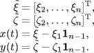
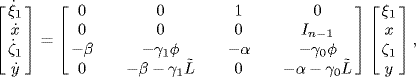
Let ξ = [ξ1, ξ2, . . . , ξn]T and ζ = [ζ1, ζ2, . . . , ζn]T. With the control protocol (6.14), the closed-loop system of can be written in the matrix form as
where
(6.16) ![]()
It is said that a consensus is asymptotically achieved in system (6.15) if |ξi − ξj| → 0 and |ζi − ζj| → 0 as t→ ∞.
To analyze the stability property of system (6.15), we first research the eigenvalues of Γ. Denote the eigenvalues of L by μ1 = 0, μ2, . . . , μn. Simple computation shows that
Writing L in upper triangular Jordan blocks with ![]() as diagonal elements, from (6.17) we get
as diagonal elements, from (6.17) we get
Thus for each μi, there exist two eigenvalues of Γ, denoted by λi1 and λi2 respectively. Since μ1 = 0, we obtain two eigenvalues λ11 and λ12 of Γ:
which are determined only by parameters of the agent. Obviously, λ11,12 = 0 if and only if α = 0, β = 0. Now, we show that the eigenvalues of Γ excluding λ11,12 determine if the consensus is achieved in system (6.15), and λ11,12 determine the dynamics of the achieved consensus solution.
Theorem 6.5 System (6.15) reaches a consensus asymptotically if and only if
(6.20) ![]()
And the dynamics of the consensus solution are determined by the equation
Proof. Let
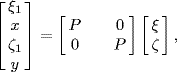
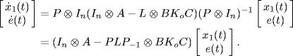
Then, the consensus is achieved asymptotically if and only if x(t) → 0 and y(t) → 0 as t→ ∞. Let the nonsingular transformation matrix P be given by (6.8). Then, we have
and
(6.23) ![]()
where ![]() was given by (6.7).
was given by (6.7).
With the linear transformation (6.22), the closed-loop system (6.15) is transformed to
or equivalently,
Hence, the consensus is achieved if and only if all the eigenvalues of
(6.25) ![]()
lie in the left-half complex plane. Since we have shown that the eigenvalues of ![]() are the remaining n − 1 eigenvalues of L excluding zero, i.e., μ2, . . . , μn (Proposition 6.1), it follows from (6.18) that the eigenvalues of
are the remaining n − 1 eigenvalues of L excluding zero, i.e., μ2, . . . , μn (Proposition 6.1), it follows from (6.18) that the eigenvalues of ![]() are exactly the remaining 2(n − 1) eigenvalues of Γ excluding λ11,12 = 0. Hence, system (6.15) reaches a consensus asymptotically if and only if Re(λij) < 0, i = 2, 3, . . . , n; j = 1, 2.
are exactly the remaining 2(n − 1) eigenvalues of Γ excluding λ11,12 = 0. Hence, system (6.15) reaches a consensus asymptotically if and only if Re(λij) < 0, i = 2, 3, . . . , n; j = 1, 2.
When x(t) → 0, y(t) → 0, from (6.24) it is clear that the dynamics of the consensus solution is determined by equation (6.21), whose eigenvalues are given by (6.19). The theorem is thus proved. ![]()
Obviously, if α > 0 and β > 0, then the consensus solution is asymptotically stable. An asymptotically stable solution is called trivial consensus solution in this book. For a trivial consensus solution, cooperation of agents is not necessary because it can be easily achieved by taking zero consensus gains, i.e., γ0 = γ1 = 0. Therefore, to achieve a non-trivial consensus we make the following assumption for system (6.13).
Assumption 6.6 In system (6.13) α ≤ 0 or β ≤ 0.
6.2.2 Consensus and Consentability Condition
Now, we study how agent parameters, protocol parameters and the Laplacian matrix determine the eigenvalues of system (6.15). According to (6.18), we need to analyze the stability of a class of quadratic polynomials with complex coefficients.
Lemma 6.7 Let ![]() . The two roots of the polynomial
. The two roots of the polynomial
lie in the open left-half complex plane if and only if
where p = Re(− μ) and q = Im(− μ).
Proof. Denote
![]()
where μ* is the conjugate of μ. It is easy to see that ![]() for any complex number λ0, which implies that
for any complex number λ0, which implies that ![]() is a root of fμ(λ) if and only if λ0 is a root of
is a root of fμ(λ) if and only if λ0 is a root of ![]() . Therefore, the complex coefficient polynomial f(λ) has no RHP roots if and only if the real coefficient polynomial
. Therefore, the complex coefficient polynomial f(λ) has no RHP roots if and only if the real coefficient polynomial ![]() has no RHP roots.
has no RHP roots.
Let a = α − pγ1, b = β − pγ0, c = qγ1 and d = qγ0. With simple calculations, we have
(6.29) ![]()
where
![]()
![]()
By Hurwitz stability criterion, all the roots have negative real parts if and only if
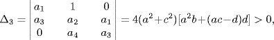
Obviously, (6.30)–(6.33) are equivalent to
In the following, we will show that (6.35) and (6.37) can be removed. With simple computation, one has
![]()
which means that (6.35) is implied by (6.36). Moreover, if b2 + d2 = 0, then b = d = 0, which is contradictory to (6.36). Therefore, each root of (6.26) has a negative real part if and only if both (6.34) and (6.36), or equivalently (6.27) and (6.28), hold. ![]()
Lemma 6.8 Assume p = Re(− μ) < 0, q = Im(− μ), γ0 ≥ 0 and α ≥ 0. Then, (6.27) and (6.28) hold if and only if
where β![]() = (β − pγ0)p − γ0q2 = βp − γ0(p2 + q2).
= (β − pγ0)p − γ0q2 = βp − γ0(p2 + q2).
Proof. If q = 0 or γ0 = 0, the lemma is obvious. We assume q ≠ 0 and γ0 ≠ 0 in the following. Since p < 0, inequality (6.27) can be rewritten as γ1 > α/p. Moreover, if (6.27) holds, then (6.28) can be rewritten as
![]()
namely,
(Necessity) Let
![]()
With simple calculations, we obtain
![]()
for all ![]() , which implies h(γ) is a decreasing function. By (6.28) we have
, which implies h(γ) is a decreasing function. By (6.28) we have
![]()
Thus, (6.38) holds and β![]() < 0. Denote by g(γ1) the left side of (6.40), which is a quadratic polynomial with respect to γ1 with coefficient β
< 0. Denote by g(γ1) the left side of (6.40), which is a quadratic polynomial with respect to γ1 with coefficient β![]() p > 0 and the discriminant
p > 0 and the discriminant
![]()
Solving (6.40) yields γ1 > ρ1 or γ1 < ρ2, where
are the two roots of polynomial g(γ1). From (6.41), we can see that ρ2 < α/p < ρ1. Thus, from γ1 > α/p, we obtain γ1 > ρ1, that is (6.39).
(Sufficiency) It is easy to see that (6.39) implies γ1 > α/p, that is, (6.27) holds. From (6.38), we have β![]() < 0, which implies β
< 0, which implies β![]() p > 0. Thus, (6.40) is obtained from γ1 > ρ1. Hence (6.28) holds.
p > 0. Thus, (6.40) is obtained from γ1 > ρ1. Hence (6.28) holds. ![]()
Remark. For the case of α ≥ 0, β = 0 and γ1 > 0, the necessary and sufficient condition of Lemma 6.8 reduces to the form:
In particular, if q = 0, then (6.42) holds for any γ1 > 0, which implies Lemma 4.2 of Ren and Atkins (2007). Let α = β = 0, γ1 > 0 and γ0 > 0. Then, (6.42) further reduces to the form:
(6.43) ![]()
which includes the sufficient condition obtained by Ren and Atkins (2007) as a special case. Let α = β = 0, p < 0 and γ1 = 1. Then, by Lemma 6.7, polynomial (6.26) is stable if and only if
(6.4) ![]()
which is just the Lemma 2 of Lin et al.(2007).
By Theorem 6.5 and Lemma 6.7, we obtain the following theorem:
Theorem 6.9 Let pi = Re(− μi) and qi = Im(− μi). Then the consensus is achieved asymptotically in system (6.13) with protocol (6.14) if and only if
Remark 1. Inequalities (6.45) and (6.46) describe all admissible parameters of system (6.13) and control gains of protocol (6.14) for consensus. If α > 0 and β > 0, conditions (6.45) and (6.46) imply that all the eigenvalues of Γ have negative real parts. In this case, the multi-agent system is asymptotically stable, in other words, it achieves the so-called trivial consensus.
Remark 2. When α ≤ 0 or β ≤ 0, then the non-trivial consensus is achieved if and only if conditions (6.45) and (6.46) hold. One may wonder why it is not assumed that the digraph G contains a globally reachable node (or equivalently say, G has a spanning tree) as stated in Ren and Beard (2005). As a matter of fact, this condition is implied by (6.45) and (6.46) as α ≤ 0 or β ≤ 0. This is shown in the necessity part of the proof of next theorem.
Theorem 6.10 Suppose that α ≤ 0 or β ≤ 0. Then, the system (6.13) is consentable under protocol (6.14) if and only if the topology graph has a globally reachable node.
Proof. (Necessity) Suppose the system (6.13) is consentable under protocol (6.14), but G has no globally reachable node. Then, by Theorem 1.9, there is a μi = 0 (i ≥ 2), i.e., pi = qi = 0. Thus (6.45) and (6.46) imply α > 0 and β > 0, which is a contradiction.
(Sufficiency) Suppose that G contains a globally reachable node. Then max 2≤i≤npi < 0. Thus, (6.45) is equivalent to
as γ1 > 0. Therefore, for any given α and γ0, there always exist sufficiently large numbers γ1 and β such that (6.47) and (6.46) hold, that is, the consensus is achieved. ![]()
When the condition that graph G contains a globally reachable node is assumed, the next theorem provides a necessary and sufficient condition for the design of control gains of the consensus protocol.
Theorem 6.11 Let pi = Re(− μi) and qi = Im(− μi). Assume γ0 ≥ 0, α ≥ 0 and graph G contains a globally reachable node. Then the consensus is achieved in system (6.13) with protocol (6.14) if and only if
where ![]() .
.
Proof. Since G contains a globally reachable node, by Theorem 1.9, we have pi < 0 for all i = 2, 3, . . . , n. Hence, by Theorem 6.5, Lemma 6.7 and Lemma 6.8, the theorem is proved. ![]()
Corollary 6.12 Assume γ0 > 0, α ≥ 0, β = 0 and graph G contains a globally reachable node. Then the consensus is achieved in system (6.13) with protocol (6.14) if and only if
(6.50) 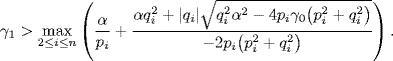
In particular, for α = β = 0, the consensus is achieved by the protocol (6.14) if and only if
Remark 1. Corollary 6.12 includes Theorem 4.2 and 4.3 of Ren and Beard (2005) as special cases. For the case of α = β = 0, Corollary 6.12 is equivalent to Theorem 1 of Lin et al. (2007).
Remark 2. From (6.19), we know that α and β determine the consensus dynamics poles. If β < 0, then one consensus pole is positive. In this case, the positive exponential consensus is also achieved. As γ0, α and β are given, γ1 determines the error dynamics poles and the convergence speed. For the problem how to choose γ1 in ![]() such that the maximum convergence speed of the error dynamics is achieved, readers are referred to Zhu, Tian and Kuang (2009).
such that the maximum convergence speed of the error dynamics is achieved, readers are referred to Zhu, Tian and Kuang (2009).
6.2.3 Periodic Consensus Solutions
By Theorem 6.5, the dynamics of the consensus solution is determined by each agent itself. Suppose that 4β − α2 > 0. Then, from (6.19) it follows that two eigenvalues of the consensus dynamics are conjugate complex numbers with real part as Reλ11 = Reλ12 = − α/2. Obviously, if α < 0, then the positive exponential consensus is achieved. If α = 0, then the periodic consensus is achieved. In particular, we let γ0 = 0, then (6.47) and (6.46) are reduced to γ1 > 0 and β > 0. For this special case, we have following theorem.
Theorem 6.13 Suppose α = γ0 = 0. Then, periodic consensus is achieved in system (6.13) with protocol (6.14) if and only if γ1 > 0, β > 0 and G has a spanning tree. Moreover, the vibration frequency of the periodic consensus dynamics is ![]() and γ1 determines the error dynamics poles.
and γ1 determines the error dynamics poles.
Proof. Substituting α = γ0 = 0 into (6.19), we obtain the consensus poles ![]() . By Theorem 6.5 and the proof of Theorem 6.10, we know that the periodic consensus is achieved if and only if γ1 > 0, β > 0 and G contains a globally reachable node. Thus the vibration frequency of the periodic consensus dynamics is
. By Theorem 6.5 and the proof of Theorem 6.10, we know that the periodic consensus is achieved if and only if γ1 > 0, β > 0 and G contains a globally reachable node. Thus the vibration frequency of the periodic consensus dynamics is ![]() . From (6.18), we know that λi1 and λi2 are the roots of λ2 + γ1μiλ + β
. From (6.18), we know that λi1 and λi2 are the roots of λ2 + γ1μiλ + β ![]() . Thus, as the vibration frequency is given, the positions of the other eigenvalues except λ11 and λ12 are determined by γ1. Therefore, the error dynamics poles are determined by γ1.
. Thus, as the vibration frequency is given, the positions of the other eigenvalues except λ11 and λ12 are determined by γ1. Therefore, the error dynamics poles are determined by γ1.![]()
6.2.4 Simulation Study
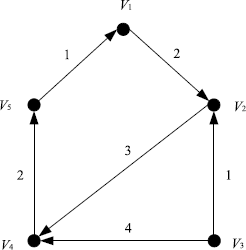
Consider the multi-agent systems with second-order agents given by (6.13) with α = 0 and digraph shown in Figure 6.1. Obviously, the Laplacian matrix of the digraph is
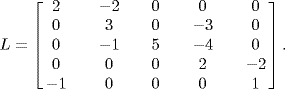
Figure 6.1 The directed graph of the multi-agent system.
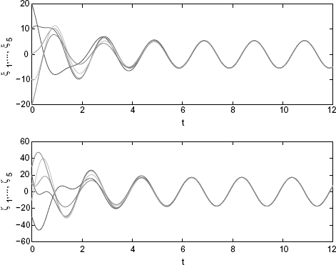
Let γ0 = 0, γ1 = 1 in the consensus protocol (6.14). Then, periodic consensus should be achieved according to Theorem 6.13 Suppose the desired period of consensus dynamics is T = 2. Then, β = (2π/T)2 by Theorem 6.13. Set the initial value vector as [ξT(0) ζT(0)]T = [20 10 0 − 10 − 20 − 30 20 10 − 10 30]T. Figure 6.2 shows the achieved periodic consensus of ξi and ζi.
Figure 6.2 The periodic consensus with desired period 2. (Reprinted from Linear Algebra and its Applications, 431, Zhu J., Tian Y.-P. and Kuang J., “On the general consensus protocol of multi-agent systems with double-integrator dynamics,” 701–715, 2009, with permission from Elsevier.)
If we regard the graph shown in Figure 6.1 as an undirected graph. Then the Laplacian matrix of G is
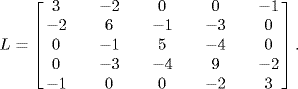
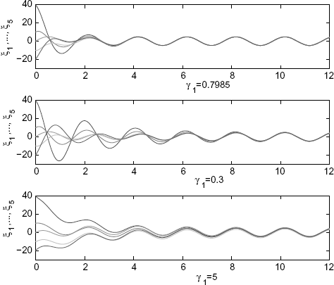
With simple calculations, we obtain μ2 = 2.7639 μ5 = 12.5826. Hence, according to Zhu, Tian and Kuang (2009), the maximum convergence speed is achieved as γ1 = 0.7985. The simulation can be seen in Figure 6.3 for different values of γ1 with the same initial value vector as [ξT(0) ζT(0)]T = [40 10 0 − 10 − 20 − 30 20 20 − 10 40]T.
Figure 6.3 The maximum convergence speed is achieved as γ1 = 0.7985. (Reprinted from Linear Algebra and its Applications, 431, Zhu J., Tian Y.-P. and Kuang J., “On the general consensus protocol of multi-agent systems with double-integrator dynamics,” 701–715, 2009, with permission from Elsevier.)
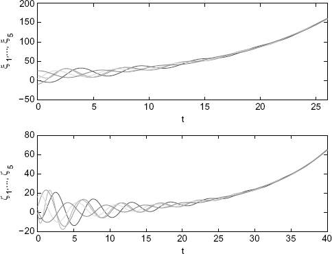
Let the directed graph be still given by Figure 6.1. Assume the desired poles of the consensus dynamics are 0.1 and −2. Then α = 1.9 > 0, β = − 0.2. With simple calculation, the right side of (6.48) is equal to 0.0571. Now, we let γ0 = 1 > 0.0571. Then the right side of (6.49) equals −0.2107. Hence, by Theorem 6.11, the positive exponential consensus is achieved for any γ1 > − 0.2107. Figure 6.4 shows the simulation for γ1 = − 0.1 and the initial value vector as [0 − 10 12 4 25 − 4 6 0 16 3]T.
Figure 6.4 The positive exponential consensus. (Reprinted from Linear Algebra and its Applications, 431, Zhu J., Tian Y.-P. and Kuang J., “On the general consensus protocol of multi-agent systems with double-integrator dynamics,” 701–715, 2009, with permission from Elsevier.)
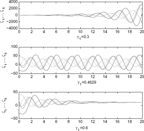
Let α = β = 0 and γ1 = 1. Then, the right side of (6.51) equals 0.4629. Hence, by Corollary 6.12, the consensus is achieved if and only if γ1 > 0.4629. Using (11) in Theorem 4.2 of Ren and Atkins (2007), one obtains γ1 > 1, which is only a sufficient condition. Figure 6.5 and Figure 6.6 show the phenomena from disagreement to the agreement.
Figure 6.5 From the disagreement to the agreement of ξi. (Reprinted from Linear Algebra and its Applications, 431, Zhu J., Tian Y.-P. and Kuang J., “On the general consensus protocol of multi-agent systems with double-integrator dynamics,” 701–715, 2009, with permission from Elsevier.)
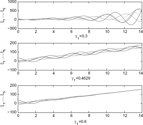
Figure 6.6 From the disagreement to the agreement of ζi. (Reprinted from Linear Algebra and its Applications, 431, Zhu J., Tian Y.-P. and Kuang J., “On the general consensus protocol of multi-agent systems with double-integrator dynamics,” 701–715, 2009, with permission from Elsevier.)
6.3 High-Order Agent System
6.3.1 System Model
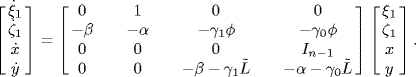
Consider a multi-agent system with n identical agents. The ith agent is a linear time-invariant (LTI) dynamic system given by
where ![]() and
and ![]() are the state, input and output of the ith agent, respectively;
are the state, input and output of the ith agent, respectively; ![]() and
and ![]() are constant matrices.
are constant matrices.
The output-based consensus protocol has the following form:
where ![]() is a gain matrix for output feedback.
is a gain matrix for output feedback.
If C = I, (6.53) becomes the following state-based consensus protocol:
where ![]() is a gain matrix for state feedback.
is a gain matrix for state feedback.
Definition 6.14 It is said that the system (6.52) with the consensus protocol (6.53) (or (6.53)) achieves a consensus asymptotically if
holds for any initial value ![]() . The system (6.52) is said to be consentable under the consensus protocol (6.53) (or (6.54)) if there is a gain matrix
. The system (6.52) is said to be consentable under the consensus protocol (6.53) (or (6.54)) if there is a gain matrix ![]() (or
(or ![]() ) such that the closed-loop system of (6.52) with (6.53) (or (6.54)) achieves a consensus asymptotically.
) such that the closed-loop system of (6.52) with (6.53) (or (6.54)) achieves a consensus asymptotically.
6.3.2 Consensus Condition
Denote
where ⊗ denotes the Kronecker product, which satisfies the following properties: (1) (A ⊗ B)(C ⊗ D) = AC ⊗ BD; (2) (A ⊗ B)T = AT ⊗ BT (Horn and Johnson (1985).
By definition (6.58) it is easy to see that (6.55) is equivalent to
![]()
In other words, the consensus is achieved asymptotically if and only if the error system with state e(t) is asymptotically stabilized. Now, let us derive the state space equation of the error system.
First, we can write the closed-loop system (6.52) with consensus protocol (6.53) as follows
where L is the Laplacian matrix of the topology graph of the system. From (6.56), (6.57) and (6.58) we have
where P was given by (6.8). With the linear transformation (6.60), the closed-loop system (6.59) is transformed into
As shown in the proof of Proposition 6.1,
![]()
where ![]() was given by (6.7). So, (6.61) can also be written as
was given by (6.7). So, (6.61) can also be written as
(6.62) ![]()
Hence, based on the upper-triangular structure of the system matrix we conclude that consensus is achieved in the system (6.52) with protocol (6.53) if and only if all the eigenvalues of the matrix
lie inside the LHP; and moreover, the dynamics of the consensus solution are determined by the equation of the open-loop system of (6.52).
In Proposition 6.1 we have shown that the eigenvalues of ![]() are the remaining n − 1 eigenvalues of L excluding zero, denoted by μ2, . . . , μn. Let us write
are the remaining n − 1 eigenvalues of L excluding zero, denoted by μ2, . . . , μn. Let us write ![]() in upper triangular Jordan blocks, T−1JT, with μ2, . . . , μn as diagonal elements of J. Then, we get the characteristic equation of matrix Γ defined by (6.63) as
in upper triangular Jordan blocks, T−1JT, with μ2, . . . , μn as diagonal elements of J. Then, we get the characteristic equation of matrix Γ defined by (6.63) as
(6.64) ![]()
Considering the upper triangular structure of J we have arrived at the following theorem.
Theorem 6.15 Consensus is achieved in system (6.52) with protocol (6.53) if and only if all the eigenvalues of ![]() lie inside the LHP. And moreover, the dynamics of the consensus solution are determined by the equation of the open-loop system of (6.52), i.e.,
lie inside the LHP. And moreover, the dynamics of the consensus solution are determined by the equation of the open-loop system of (6.52), i.e.,
![]()
where ![]() .
.
To avoid the so-called trial consensus solution we make the following assumption for system (6.52).
Assumption 6.16 In system (6.52) A is not a Hurwitz matrix.
6.3.3 Consentability
Theorem 6.15 also implies that system (6.52) is consentable under protocol (6.53) if and only if n − 1 systems (A, μiB, C) (or (A, B, μiC)), ![]() , can be simultaneously stabilized by an output feedback controller.
, can be simultaneously stabilized by an output feedback controller.
Since we have assumed that A is not a Hurwitz matrix, the consentability implies that each system (A, μiB, C) or (A, B, μiC) is stabilizable by output feedback, which further implies that (A, μiB) is stabilizable and (C, A) is detectable (or, (A, B) is stabilizable and (A, μiC) is detectable). Obviously, in any case μi ≠ 0 is a necessary condition. By Theorem 1.9 we know that μi ≠ 0, ![]() , only if the topology graph of the system contains at least one globally reachable node. So, the following proposition is obviously true.
, only if the topology graph of the system contains at least one globally reachable node. So, the following proposition is obviously true.
Proposition 6.17 If system (6.52) is consentable under protocol (6.53), then the topology graph G contains a globally reachable node.
Noticing that for any non-zero ![]() , the stabilizability of (A, μiB) is equivalent to the stabilizability of (A, B), and the detectability of (A, μiC) is equivalent to the detectability of (A, C). So, considering Proposition 6.17 the following proposition is also obviously true.
, the stabilizability of (A, μiB) is equivalent to the stabilizability of (A, B), and the detectability of (A, μiC) is equivalent to the detectability of (A, C). So, considering Proposition 6.17 the following proposition is also obviously true.
Proposition 6.18 If system (6.52) is consentable under protocol (6.53), then (A, B) is stabilizable and (A, C) is detectable.
Propositions 6.17 and 6.18 provide necessary conditions of the consentability of system (6.52) under protocol (6.53). Now, let us further try to find some necessary and sufficient conditions.
The open-loop transfer function matrix of each agent is
where ![]() , are the n − 1 eigenvalues of the Laplacian matrix L except the first zero eigenvalue corresponding to the eigenvector 1n. Then, an equivalent formulation of the consentability problem is given as follows.
, are the n − 1 eigenvalues of the Laplacian matrix L except the first zero eigenvalue corresponding to the eigenvector 1n. Then, an equivalent formulation of the consentability problem is given as follows.
Simultaneous stabilization problem:
Does there exist a ![]() such that all the systems given by (6.65) can be simultaneously stabilized by a common output feedback controller
such that all the systems given by (6.65) can be simultaneously stabilized by a common output feedback controller
(6.66) ![]()
Now, we first study this problem for the case when the topology graph is undirected. In this case, by Theorem 1.9, all the eigenvalues of Laplacian matrix L are non-negative real numbers, which in an ascending order are written as 0 = μ1 ≤ μ2 ≤ ![]() ≤ μn.
≤ μn.
Suppose G(s) = C(sI − A)−1B is output stabilizable and U(s) = − K0Y(s) is such an output feedback stabilizer. By the continuity of the system poles on entries of K0, there exists an interval (κ1, κ2) such that G(s) is stabilized by U(s) = − γK0Y(s) for all γ ![]() (κ1, κ2), i.e., the equation
(κ1, κ2), i.e., the equation
![]()
has no RHP zero. Let ![]() and
and ![]() be the extreme values of κ1 and κ2 respectively, i.e., for all
be the extreme values of κ1 and κ2 respectively, i.e., for all ![]() , γK0 stabilizes G(s), but both
, γK0 stabilizes G(s), but both ![]() and
and ![]() marginally stabilize G(s). Denote
marginally stabilize G(s). Denote
(6.67) ![]()
Then, we have the following theorem.
Theorem 6.19 Suppose that
Then system (6.52) is consentable under protocol (6.53) if and only if the undirected topology graph G is connected.
Proof. Necessity is already ensured by Proposition 6.17 We need to just prove the sufficiency. Since G is connected, ![]() . By (6.68) we can find an
. By (6.68) we can find an ![]() > 0 such that
> 0 such that ![]() . Take
. Take ![]() . Then,
. Then, ![]() ,
, ![]() . Hence, the equation
. Hence, the equation
![]()
has no RHP zeros for all ![]() .
. ![]()
When ![]() can be arbitrarily large (high-gain stabilizable) or
can be arbitrarily large (high-gain stabilizable) or ![]() can be arbitrarily small (low-gain stabilizable), rop→ ∞ and hence, (6.68) always holds. So, the following corollary of Theorem 6.19 is obvious.
can be arbitrarily small (low-gain stabilizable), rop→ ∞ and hence, (6.68) always holds. So, the following corollary of Theorem 6.19 is obvious.
Corollary 6.20 Suppose that system (A, B, C) is high-gain output stabilizable or low-gain output stabilizable. Then, system (6.52) is consentable under protocol (6.53) if and only if its undirected topology graph is connected.
The following lemma given in Dragan and Hahalany (1999) shows that a square minimum phase system is high-gain stabilizable.
Lemma 6.21 Suppose system (A, B, C) satisfies
(6.69) ![]()
Let H be a matrix whose eigenvalues satisfies Re[λ] ≤ − 2α1 < 0. Then, there exists ε0 > 0 such that for arbitrary ε ![]() (0, ε0) and some c > 0 independent of ε, the state and the output of the closed-loop system (A, B, C) with output feedback
(0, ε0) and some c > 0 independent of ε, the state and the output of the closed-loop system (A, B, C) with output feedback ![]() satisfy
satisfy
![]()
By Definition 2.11, condition (1) in Lemma 6.21 implies that the system (A, B, C) ia square and has relative degree as one, and condition (2) implies that the system (A, B, C) is minimum phase. From the above lemma and Corollary 6.20 we directly obtain the following theorem on consentability.
Theorem 6.22 Suppose square system (A, B, C) is minimum phase and CB is invertible. Then, system (6.52) is consentable under protocol (6.53) if and only if the topology graph G is connected.
Next, we will extend the conclusion given by Corollary 6.20 to the case when the interconnection topology graph is directed. In this case, by Theorem 1.9, all the eigenvalues of Laplacian matrix L have non-negative real parts, i.e., ![]() , and 0 = μ1 ≤ Re(μ2) ≤
, and 0 = μ1 ≤ Re(μ2) ≤ ![]() ≤ Re(μn).
≤ Re(μn).
Suppose ![]() , where
, where ![]() . Denote
. Denote
(6.70) ![]()
(6.71) ![]()
(6.72) 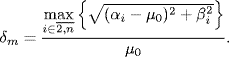
Then, we have
(6.73) ![]()
(6.74) ![]()
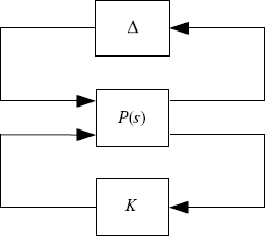
Then, the simultaneous stabilization problem is solvable if the following robust stabilization problem is solvable.
Robust stabilization problem:
For any Δ satisfying ||Δ||∞ ≤ δm, does there exist a ![]() such that the uncertain system σ(I + Δ)G(s) can be robustly stabilized by the output feedback controller U(s) = − KY(s)?
such that the uncertain system σ(I + Δ)G(s) can be robustly stabilized by the output feedback controller U(s) = − KY(s)?
This robust stabilization problem is sketched in Figure 6.7, where
![]()
By the robust control theory (Feng, Tian and Xin (1996); Zhou, Doyle and Glover (1996), the problem is solvable if there exists a ![]() such that
such that
Suppose that the topology digraph G contains a globally reachable node. Then, |μi| ≠ 0 for all ![]() , which implies that δm< ∞. If G(s) is low-gain output stabilizable, then there exists an
, which implies that δm< ∞. If G(s) is low-gain output stabilizable, then there exists an ![]() such that G(s) can be stabilized by U(s) = − κK0Y(s), where
such that G(s) can be stabilized by U(s) = − κK0Y(s), where ![]() can be arbitrarily close to zero. So, in this case we can always find a K = κK0 such that (6.75) holds, because
can be arbitrarily close to zero. So, in this case we can always find a K = κK0 such that (6.75) holds, because
![]()
when κ → 0. Therefore, we have proved the following theorem.
Figure 6.7 Robust stabilization problem.
Theorem 6.23 Suppose that system (A, B, C) is low-gain output stabilizable. Then, system (6.52) is consentable under protocol (6.53) if and only if its topology digraph contains a globally reachable node.
The system (A, B) is low-gain stabilizable by state feedback if the system is stabilizable and all the eigenvalues of A are in the closed LHP (Lin (1998). Based on this fact we have the following theorem on consentability.
Theorem 6.24 Suppose all the eigenvalues of A are in the closed LHP. Then, system (6.52) is consentable under protocol (6.54) if and only if its topology digraph G contains a globally reachable node and (A, B) is stabilizable.
Now, we study high-gain output stabilizable systems for the case when the interconnection topology is directed.
If (A, B) is stabilizable, then by linear system theory (Cheng and Ma (2006), the Riccati equation
has a unique semi-positively definite solution P. If the following rank condition holds
then the matrix equation XC = BTP has at least a solution denoted by K0, i.e.,
Then, the system (A, B, C) can be stabilized by output feedback u = − γK0y for arbitrary γ ![]() [1, ∞), i.e., the system is high-gain stabilizable (Ma (2009). This can be proved by taking a Lyapunov function V(x) = xTPx for that closed-loop system. The derivative of the Lyapunov function is
[1, ∞), i.e., the system is high-gain stabilizable (Ma (2009). This can be proved by taking a Lyapunov function V(x) = xTPx for that closed-loop system. The derivative of the Lyapunov function is
It can be further shown that under the condition (6.77), the system (A, μB, C) or (A, B, μC) with ![]() is also high-gain stabilizable. In this case, since the system contains a complex parameter, the state of the system is a vector in
is also high-gain stabilizable. In this case, since the system contains a complex parameter, the state of the system is a vector in ![]() . So, we can take a Lyapunov function as V = x*Px, where x* is the conjugate transpose of x. Then, under the output feedback u = − γK0y, where K0 satisfies (6.78), the derivative of the Lyapunov function along the system solution is
. So, we can take a Lyapunov function as V = x*Px, where x* is the conjugate transpose of x. Then, under the output feedback u = − γK0y, where K0 satisfies (6.78), the derivative of the Lyapunov function along the system solution is
![]()
Obviously, ![]() as long as
as long as ![]() .
.
Therefore, we have the following theorem on consentability, which was first obtained in Ma and Zhang (2010).
Theorem 6.25 Suppose Riccati equation (6.76) has a positively semi-definite solution P such that (6.77) holds. Then, system (6.52) is consentable under protocol (6.53) if and only if the topology digraph G contains a globally reachable node and (A, B) is stabilizable.
By doing the following exercise the reader will understand that under the condition (6.77) the system (A, B, C) is minimum phase.
Exercises 6.26 Suppose (A, B) is stabilizable and P is the solution of the Reccati equation (6.76). Show (A, B, C) is minimum phase if the rank condition (6.77) holds.
Note that when state feedback consensus protocol is used, i.e., C = I, then the rank condition (6.77) automatically holds. We have the following corollary of Theorem 6.25.
Theorem 6.27 System (6.52) is consentable under protocol (6.54) if and only if the topology digraph G contains a globally reachable node and (A, B) is stabilizable.
6.4 Notes and References
Consensus problems have a long history in statistics (DeGroot 1974), distributed computation (Bertsekas, and Tsitsiklis 1989; Cybenko 1989; Lynch 1997) and distributed estimation (Borkar and Varaiya 1982). Consensus is also one of fundamental principles in the design of sensor networks (Kar and Moura 2008, (2009) and multi-robot coordination control systems (Cortijés et al. 2004; Fax and Murray 2004; Olfati-Saber, Fax and Murray 2007). Vicsek et al. (1995) proposed a discrete-time model of multi-autonomous agents, and demonstrated that without any central control, all the agents move in the same direction when the density is large and the noise is small. Jadbabaie, Lin and Morse (2003) studied the linearized Vicsek's model and proved that all the agents converge to a common steady state provided that the interconnection graph is jointly connected. Based on algebraic graph theory, Olfati-Saber and Murray (2003), (2004) analyzed the consensus problem for networks of first-order integrator agents with fixed and switching topologies, and showed that the consensus can be achieved under the assumption of strong connection of digraphs. Moreau (2005), Ren and Beard (2005) generalized the results of Jadbabaie, Lin and Morse (2003), Olfati-Saber and Murray (2004), and in particular, Ren and Beard (2005), presented a more relaxed condition of the solvability of the consensus problem, i.e., the existence of a spanning tree in the topology digraph. Similar results were obtained by Lin, Francis and Maggiore (2005). Some special second-order consensus protocols were proposed and some sufficient consensus conditions were obtained by (Lin et al. 2007; Ren and Atkins 2007). In particular, Ren and Atkins (2007) proposed two kinds of second-order consensus protocols, under which the state of each agent converges to a constant or a linear function with respect to the time.
Section 6.3 tries to unify most results on consensus seeking ability (or consentabilty in this book) in the framework of high-gain and low-gain stabilization.
The consensus seeking ability problem of multi-agent systems (MASs) with continuous-time high-order LTI dynamic agents was investigated by Wang, Cheng and Hu (2008), Xiao and Wang (2007) and Seo et al. (2009), which showed that for the system with semi-stable agents the problem is solvable if the interconnection topology has a globally reachable node. This result basically relies on the low-gain stabilizability of semi-stable systems (Lin (1998), (2009). Zhang and Tian (2010), (2012) extended such results to stochastic MASs.
The word “consentability” appeared for the first time in the work Zhang and Tian (2009). It introduced the concept of consentability under two kinds of second-order consensus protocols. For discrete MASs with double-integrator dynamics, Zhang and Tian (2009) obtained necessary and sufficient conditions of the consentability for fixed and stochastic switching topologies. The results of Zhang and Tian (2009) much benefit from the technique shown by Proposition 6.1 and Theorem 6.2, which successfully converts the consensus problem of the original MAS into an ordinary stability problem of a reduced-order system, and hence the consentability problem to a stabilizability problem. Using this technique and the Routh-Hurwitz stability criterion, Zhu, Tian and Kuang (2009) obtained a necessary and sufficient condition for the consensus of general second-order continuous-time MASs, which forms the main body of Section 6.2. Ma and Zhang (2010) used the same technique to handle the consentability problem of MASs with high-order LTI dynamic agents. (By the way, the manuscript of Zhang and Tian (2009) was sent to one of the authors of Ma and Zhang (2010) before its publication for academic exchange.) The main contribution of Ma and Zhang (2010) includes uncovering the link of the high-gain stabilization technique to the consentability problem and gives a constructive condition of the high-gain stabilization of continuous-time LTI systems based on the Riccati equation. Compared with the high-gain stabilization condition of Dragan and Hahalany (1999), this condition is less conservative because it does not require that the open system be square and has the relative degree as one; moreover, it is applicable to systems with a complex-number parameter. Ma and Zhang (2010) also pointed out that such a high-gain technique is not applicable to discrete-time systems. Generally, discrete-time LTI systems is neither low-gain stabilizable nor high-gain stabilizable even under state feedback. You and Xie (2010) noticed the work of Ma and Zhang (2010) and gave a necessary and sufficient condition of the consentability of discrete-time MASs with high-order SISO agents with the help of a crucial tool developed in Fu and Xie (2005). For discrete-time MASs with MIMO agents Zhang and Tian (2012) gave a sufficient condition of consentability and extended the result to stochastic MASs.
MASs with identical agents and uniform communication delays (see, e.g., Cao, Morse and Anderson 2006; Olfati-Saber and Murray 2004) are also homogeneous systems. But, just as in many other control problems, the compromise between delays and gains rather than the consentability problem occupies the central place in the analysis and design of such systems. So, they are not included in this chapter, but left to the next chapter as special cases of heterogeneous systems with diverse delays.
Bertsekas DP and Tsitsiklis JN (1989). Parallel and Distributed Computation: Numerical Methods. Prentice-Hall, Upper Saddle River, NJ. 1989
Borkar V and Varaiya P (1982). Asymptotic agreement in distributed estimation. IEEE Transactions on Automatic Control, AC-27(3), 650–655.
Cheng Z and Ma S (2006). Linear System Theory. Science Press, Beijing.
Cao M, Morse AS and Anderson BDO (2006). Reaching an agreement using delayed information. IEEE Conference on Decision and Control, San Diego, CA, USA, 3375–3380.
Cortés J, Martinez S, Karatas T, and Bullo F (2004). Coverage control for mobile sensing networks. IEEE Transactions on Robotics and Automation, 20(2), 243–255.
Cybenko G (1989). Load balancing for distributed memory multiprocessors. Journal of Parallel and Distributed Computing, 7(2), 279–301.
DeGroot MH (1974). Reaching a consensus. Journal of American Statistical Association, 69(345), 118–121.
Dragan V and Halanay A (1999). Stabilization of Linear Systems. Birkhäuser, Boston.
Fax JA and Murray RM (2004). Information flow and cooperative control of vehicle formations. IEEE Transactions on Automatic Control, 49, 1465–1476.
Feng C-B, Tian Y-P and Xin X (1996). Robust Control System Design (in Chinese). Southeast University Press, Nanjing.
Fu M and Xie L (2005). The sector bound approach to quantized feedback control. IEEE Transactions on Automatic Control, 50(11), 1698–1711.
Horn RA and Johnson CR (1985). Matrix analysis, 1st edn. Cambridge University Press, New York.
Jadbabaie A, Lin J and Morse AS (2003). Coordination of groups of mobile autonomous agents using nearest neighbor rules. IEEE Transactions on Automatic Control, 48, 988–1001.
Kar S and Moura J (2008). Sensor networks with random links: Topology design for distributed consensus. IEEE Transactions on Signal Processing, 56(7), 3315–3326.
Kar S and Moura J (2009). Distributed consensus algorithms in sensor networks with imperfect communication: Link failures and channel noise. IEEE Transactions on Signal Processing, 57(1), 355–369.
Lin P, Jia Y, Du J and Yuan S (2007). Distributed consensus control for second-order agents with fixed topology and time-delay. Proceeding of the 26th Chinese Control Conference, Zhangjiajie, Hunan, China, 577–581.
Lin Z, Francis B and Maggiore M (2005). Necessary and sufficient graphical conditions for formation control of unicycles. IEEE Transactions on Automatic Control, 50, 121–127.
Lin Z (1998). Low Gain Feedback. Lecture Notes in Control and Information Sciences, 240, Springer, London.
Lin Z (2009). Low gain and low-and-high gain feedback: a review and some recent results. Proceedings of 2009 Chinese Control and Decision Conference, lii–lxi, Guilin, China.
Lynch NA (1997). Distributed Algorithms. Morgan Kaufmann, San Francisco.
Ma C (2009). System analysis and control synthesis of linear multi-agent systems. Ph.D. dissertation, Academy of Mathematics and System Sciences, Chinese Academy of Sciences, Beijing.
Ma C and Zhang J (2010). Necessary and sufficient condition for consensusability of linear multi-agent systems. IEEE Transactions on Automatic Control, 55, 1263–1268.
Moreau L (2005). Stability of multiagent systems with time-dependent communication links. IEEE Transactions on Automatic Control, 50, 169–182.
Olfati-Saber R and Murray RM (2003). Consensus protocols for networks of dynamic agents. Proceedings of American Control Conference, 951–956.
Olfati-Saber R and Murray RM (2004). Consensus problems in networks of agents with switching topology and time-delays. IEEE Transactions on Automatic Control, 49, 1520–1533.
Olfati-Saber R and Murray RM (2006). Flocking for multi-agent dynamic systems: algorithms and theory. IEEE Transactions on Automatic Control, 51, 401–420.
Olfati-Saber R, Fax JA and Murray RM (2007). Consensus and cooperation in networked multi-agent systems. Proceedings of the IEEE, 95(1), 215–223.
Ren W and Beard RW (2005). Consensus seeking in multiagent systems under dynamically changing interaction topologies. IEEE Transactions on Automatic Control, 50, 655–661.
Ren W and Atkins E (2007). Distributed multi-vehicle coordinated control via local information exchange. International Journal of Robust and Nonlinear Control, 17, 1002–1033.
Seo JH, Shim H and Back J (2009). Consensus of high-order linear systems using dynamic output feedback compensator: low gain approach. Automatica, 45, 2659–2664.
Vicsek T, Czirok A, Ben Jacob E, et al. (1995). Novel type of phase transitions in a system of self-driven particles. Physical Review Letters, 75, 1226–1229.
Wang J, Cheng D and Hu X (2008). Consensus of multi-agent linear dynamic systems. Asian Journal of Control, 10, 144–155.
Xiao F and Wang L (2007). Consensus problems for high-dimensional multi-agent systems. IET Control Theory and Applications, 1, 830–837.
You K and Xie L (2010). Consensusability of discrete-time multi-agent systems via relative output feedback. Proceedings of the 11th International Conference on Control, Automation, Robotics and Vision, Singapore, 1239–1244.
Zhang Y and Tian Y-P (2009). Consentability and protocol design of multi-agent systems with stochastic switching topology. Automatica, 45, 1195–1201.
Zhang Y and Tian Y-P (2010). Consensus of data-sampled multi-agent systems with random communication delay and packet loss. IEEE Transactions on Automatic Control, 55(4), 939–943.
Zhang Y and Tian Y-P (2012). Maximum allowable loss probability for consensus of multi-agent systems over random weighted lossy networks. IEEE Transactions on Automatic Control, in press.
Zhou K, Doyle JC and Glover K (1996). Robust and Optimal Control. Prentice-Hall, Upper Saddle River, NJ.
Zhu J, Tian Y-P and Kuang J (2009). On the general consensus protocol of multi-agent systems with double-integrator dynamics. Linear Algebra and its Applications, 431, 701–715.