


Fabric administration
This chapter covers zoning, Fibre Channel Routing (FCR), the use of syslog, and Network Time Protocol (NTP) servers. The chapter also covers some typical SAN administration practices and techniques.
This chapter includes the following sections:
10.1 Administration practices
Many sources of documentation are available to assist with administration of a fabric for IBM b-type switches and fabrics. A defined management strategy within your organization will improve usability, speed time to implementation of new resources and changes, and reduce time to resolution of unplanned events.
The best resources for the creation and investigation of administration policies, tasks, and problem determination are this publication and others on the IBM Redbooks web site, the Fabric OS administration guides, and various topic-specific guides offered at the following websites:
A simple way to create a SAN diagram and inventory of your organization’s storage area network is to use the b-type SAN Health Assessment tool. For more information, see 12.6, “SAN health” on page 311.
Setting up items such as audit log capture (see 10.3, “Audit and syslog configuration” on page 255), network time protocol server connections (see 10.4, “Network Time Protocol” on page 259), and user IDs (see Chapter 4, “IBM Network Advisor” on page 49) are a few of the techniques that will maximize the SAN resources and provide valuable information. These techniques illustrate a few of the good administration policies that are contained in the Fabric OS administration guides and IBM Redbooks publications.
For more IBM Network Advisor topics such as installation, configuration of backups, and user management, see Chapter 4, “IBM Network Advisor” on page 49.
10.2 Initial setup
Zoning enables you to partition a storage area network (SAN) into logical groups of devices that can access each other.
Before you configure any IBM SAN switch, it must be physically assembled, racked, and connected to the appropriate electrical outlet and network. The hardware requirements and specifications can be found in the specific b-type hardware installation guide that comes with the product.
After the SAN switch is physically installed and powered on, some initial configuration parameters must be set. All of the b-type switches require the same initial setup. The fundamental steps have not changed from the earlier switch models.
For information about initial installation and configuration, see the installation, service, and user guides for your switch at the IBM product support portal:
|
Note: EZSwitchSetup is an easy-to-use graphical user interface application for setting up and managing single switch fabrics.
For full compatibility, see the EZSwitchSetup Administrator’s Guide, which you can download at the following website:
|
10.3 Audit and syslog configuration
The b-type audit log and syslog provide valuable information about what has occurred on a switch and in the fabric.
The last 1024 messages are persistently saved in the audit log, but all audit events are sent to the system message log, which (assuming there are no bottlenecks) will be forwarded to your syslog server.
Audit logging assumes that your syslog is operational and running. Before configuring an audit log, ensure that the host syslog is operational and configured to preserve audit log entries past the 1024 message limit. See 10.3.2, “Syslog” on page 256 for more information.
10.3.1 Audit log
The audit log is a collection of information that is created when specific events are identified on an IBM b-type platform. The log can be dumped by running auditdump command-line interface (CLI) command, and audit data can also be forwarded to a syslog server for centralized collection.
Information is collected about many different events that are associated with zoning, security, trunking, Fibre Channel over IP (FCIP), FICON, and so on. Each release of the Fabric Operating System (FOS) provides more audit information.
By default, all event classes are configured for audit. To create an audit event log for specific events, you must explicitly set a filter. See the Fabric OS administration and the Fabric OS command guides for specific commands to set filters at. These guides are available at the following website:
Information is related to event classes tracked and made available. For example, you can track changes from an external source by the user name, IP address, or type of management interface that is used to access the switch.
To view the audit log in IBM Network Advisor, select Monitor → Logs → Audit to display the Audit log window.
Figure 10-1 shows the menu selection to open the Audit log and the opened Audit log.
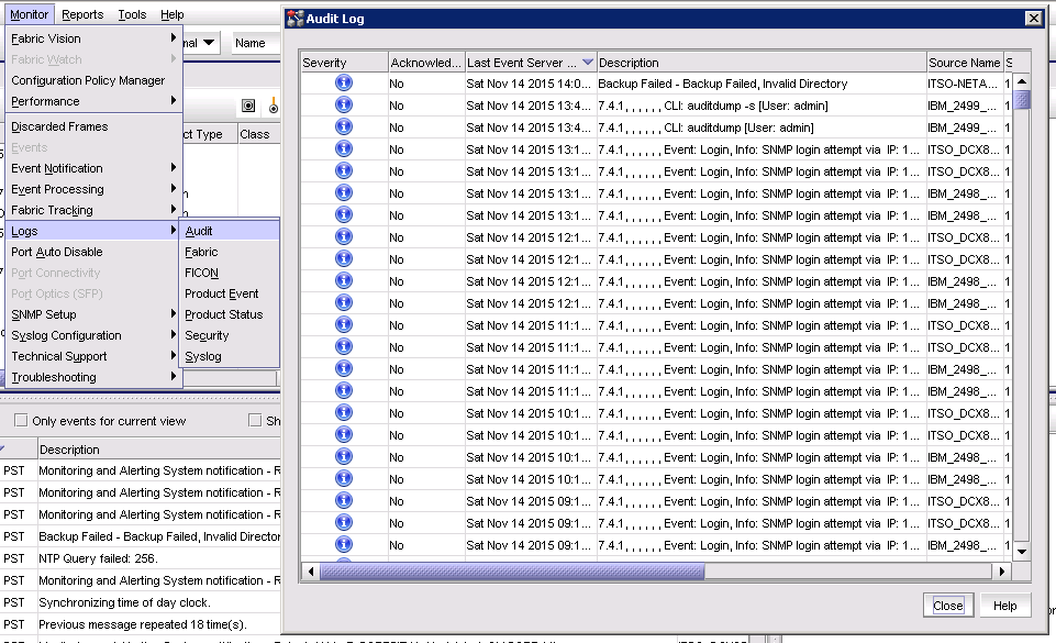
Figure 10-1 Menu section to open Audit log and open audit log pane
10.3.2 Syslog
Fabric OS 7.4.0 supports these functions:
•Configuring a switch to forward all error log entries to a remote syslog server
•Setting the syslog facility to a specified log file
•Removing a syslog server,
•Displaying the list of configured syslog servers
Brocade switches use the syslog daemon. Up to six servers are supported.
By default, the switch uses the User Datagram Protocol (UDP) to send the error log messages to the syslog server. The default UDP port is 514. However, you can configure the switch to send the error log messages securely by using the Transport Layer Security (TLS) protocol.
For more information, see Chapter 4, “IBM Network Advisor” on page 49.
Setting the syslog recipient
To automatically register the IBM Network Advisor Management application server as the syslog recipient on all managed SAN products, complete the following steps:
1. Start IBM Network Advisor.
1. Select Server → Options.
2. In the Options window, select Syslog Registration from the Category pane.
3. Select Auto register server as syslog recipient.
Figure 10-2 shows the Options window with the Syslog Registration category selected.
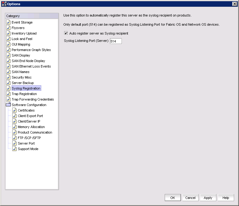
Figure 10-2 Syslog Registration panel
|
Note: The syslog listening port number is 514 in the default settings. If you change the port number to something else, auto-registration is disabled.
|
Syslog forwarding
This section describes the process of configuring the syslog server connection by using IBM Network Advisor Management server. The procedure can also be completed by using the CLI. For CLI instructions and examples, see the Fabric OS Administrators Guide and Fabric OS Command Reference at the following website:
Complete the following steps in IBM Network Advisor to perform syslog forwarding:
1. Select Monitor → Syslog Configuration → Syslog Forwarding. The Syslog Forwarding window is displayed.
4. In the Add Syslog Destination window, enter a name and the IP for the syslog server.
5. Select Syslog Repeater if you want to forward all syslogs, whether the source is managed or unmanaged. If the Syslog Repeater check box is not selected, syslogs from the managed products are sent to the server. If no filter is selected, then syslogs from all products are sent.
Figure 10-3 shows the Add Syslog Destination window.
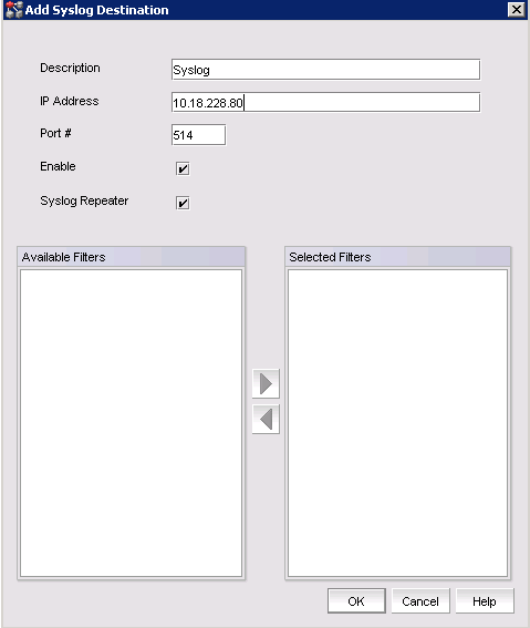
Figure 10-3 Add Syslog Destination window
6. Click OK to add the syslog destination.
While enabling secure syslog mode, you must specify a port that is configured to receive the log messages from the switch.
You are retuned to the Syslog Forwarding window.
7. Choose not to select a filter (zero) or you can select up to five filters from the Available Filters window. Click the right arrow button to move them to the Selected Filters list. This selection is enabled only when Syslog Repeater is not selected.
|
Note: When configuring filters, define them before you add the syslog server to make them available during configuration. For information about defining filters, see the Network Advisor SAN User Manual at the following website:
|
8. Select OK to close and apply the settings.
Figure 10-4 shows the Syslog Forwarding window with the syslog server added.
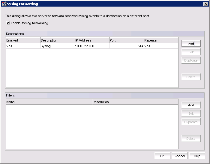
Figure 10-4 Syslog Forwarding window
10.4 Network Time Protocol
Switches maintain the current date and time internally and receive the time from the fabric’s principal switch.
Switches with incorrect date and time values work. However, because the date and time are used for logging, error detection, and troubleshooting, synchronizing the local time of the principal or primary FCS switch with at least one external Network Time Protocol (NTP) server is preferred.
If the Virtual Fabrics feature is enabled, the switch behavior has these characteristics:
•All switches in a chassis must be configured for the same set of NTP servers. This configuration ensures that time does not go out of sync in the chassis. It is not recommended to configure the local server (LOCL) in the NTP server list.
•Default switches in the fabric can query the NTP server. If Virtual Fabrics is not enabled, only the principal or primary FCS switch can query the NTP server.
•Logical switches in a chassis receive clock information from the default logical switch, and not from the principal or primary Fabric Configuration Server (FCS) switch.
Complete the following steps to synchronize the local time with NTP:
1. Log in to the switch by using the CLI.
2. Enter the tsClockServer command:
switch:admin> tsclockserver "<ntp1;ntp2>"
In the syntax, ntp1 is the IP address or DNS name of the first NTP server, which the switch must be able to access. The value ntp2 is the name of the second NTP server and is optional. The entire operand “<ntp1;ntp2>” is optional. By default, this value is LOCL, which uses the local clock of the principal or primary switch as the clock server.
switch:admin> tsclockserver
LOCL
switch:admin> tsclockserver "132.163.135.131"
switch:admin>
switch:admin> tsclockserver
132.163.135.131
switch:admin>
|
Note: NTP configuration is also available in IBM Network Advisor by using Configuration and Operational Monitoring Policy Automation Services Suite (COMPASS), which is supported in Professional Plus and Enterprise editions only. For more information about COMPASS, see the Brocade Network Advisor SAN User Manual at:
|
10.5 Zoning
Zoning enables you to partition a SAN into logical groups of devices that can access each other.
A device in a zone can communicate only with other devices that are connected to the fabric within the same zone. A device that is not included in the zone is not available to members of that zone. When zoning is enabled, devices that are not included in any zone configuration are inaccessible to all other devices in the fabric.
Using no fabric zoning is the least desirable zoning option because it allows devices to have unrestricted access on the fabric. Additionally, any device that is attached to the fabric, intentionally or maliciously, likewise has unrestricted access to the fabric. This form of zoning should be utilized only in a small and tightly controlled environment.
When using a mixed fabric (that is, a fabric that contains two or more switches running different fabric operating systems), use the switch with the highest FOS level to perform zoning tasks.
When zone or Fabric Assist (FA) zone members are specified by fabric location only (domain or area), or by device name only (node name or port worldwide name (WWN)), zone boundaries are enforced at the hardware level. In these cases, the zone is referred to as a hard zone. When zone members are specified by fabric location (domain or area) and other members of the same zone are specified by device name (node name or port WWN), zone enforcement depends on Name Server lookups. This type of zone is referred to as a soft zone.
10.5.1 Zoning preferred practices
Consider the following preferred practices when you use zoning:
•Zone using the core switch in preference to using an edge switch.
•Zone using a backbone instead of a switch. A backbone has more resources to handle zoning changes and implementations.
•Zone by single host bus adapter (HBA) where practical (see Figure 10-5) unless Peer zoning is in use (see 10.5.2, “Peer Zoning” on page 262). Each zone that is created has only one HBA (initiator) in the zone, and each target device is added to the zone. Typically, a zone is created for the HBA and the disk storage ports are added. In this manner, zone changes affect the smallest possible number of devices, minimizing the impact of an incorrect zone change.
– If the HBA also accesses tape devices, a second zone is created with the HBA and associated tape devices in it.
– For clustered systems, it might be appropriate to have an HBA from each of the cluster members included in the zone.
•When you add a switch to an existing fabric, before joining the fabric, set the default zone (defzone) policy of the switch being added as follows:
– If the joining switch has locally attached devices that are online, the defzone policy of the switch being added should be set to No Access.
– If the joining switch has no online locally attached devices, the defzone policy of the switch being added can be set to All Access.
|
Important: This setting is required to prevent a transitional state where the All Access policy might allow excessive registered state change notification (RSCN) activity. Extreme cases might create the potential for more adverse effects. This setting is for fabrics that have a very high device count.
|
Figure 10-5 shows examples of preferred zoning practices.
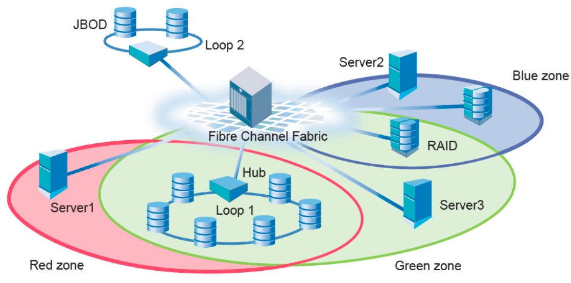
Figure 10-5 Preferred zoning practices
10.5.2 Peer Zoning
Peer Zoning allows a “principal” device to communicate with the rest of the devices in the zone. The principal device manages a Peer Zone. Other “non-principal” devices in the zone can communicate with the principal device only. They cannot communicate with each other.
Before the introduction of Peer Zoning, Single-Initiator Zoning was considered a more efficient zoning method in terms of hardware resources and RSCN volume. However, the added storage requirements of defining a unique zone for each host and target rapidly exceeds zone database size limits. As the number of zones increase, it becomes more difficult to configure and maintain the zones.
In a Peer Zone setup, principal to non-principal device communication is allowed, but non-principal to non-principal device and principal to principal device communication are not allowed. This approach establishes zoning connections that provide the efficiency of Single-Initiator Zoning with the simplicity and lower memory characteristics of One-to-Many Zoning. Figure 10-6 shows a comparison of traditional and peer zoning.
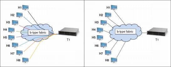
Figure 10-6 Comparison of traditional zoning (left) and peer zoning (right)
Peer Zone connectivity rules
Peer Zoning adheres to the following connectivity rules:
•Non-principal devices can communicate only with the principal device.
•Non-principal devices cannot communicate with other non-principal devices, unless allowed by some other zone in the active zone set.
•Principal devices cannot communicate with other principal devices, unless allowed by some other zone in the active zone set.
•The maximum number of Peer Zones is determined by the zone database size. The supported maximum zone database size is 2 MB for systems that are running only IBM System Storage SAN768B-2 and SAN384B-2 platforms, and their predecessors. The presence of any other platform reduces the maximum zone database size to 1 MB.
Peer Zone configuration
In the Peer Zone, devices must be identified as either WWN or D,I devices. Mixing WWN and D,I device identification within a single Peer Zone is not allowed. Aliases are not supported as devices for a Peer Zone.
|
Note: To create a peer zoning by using the CLI see the Fabric OS Administrators Guide for version 7.4 and later at the following website:
|
To create a Peer Zone by using IBM Network Advisor, complete the following steps:
1. In the IBM Network Advisor window, select Configure → Zoning → Fabric to display the Zoning window.
2. Select the correct zoning scope from Zoning Scope menu. (For more information about selecting the most appropriate scope, see “Zoning preferred practices” on page 261.
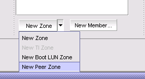
Figure 10-7 New Peer Zone pull-down option
4. Provide a meaningful name for the new Peer zone in the Peer Zone Name field.
5. Select a principal device or devices from the Potential Members pane and click the upper right facing arrow (see Figure 10-8 on page 264) to add it to the Principal Members pane.
6. Select an additional device or devices in the Potential Members pane and click the lower right facing arrow to add them to the Peer Members pane (see Figure 10-8 on page 264).
7. Click OK to create the peer zone and return to the Zoning panel.
The peer zone now appears in the list of available zones that can be added to a zoning configuration and activated in the Zoning panel.
Figure 10-8 shows the Add Peer Zone window.
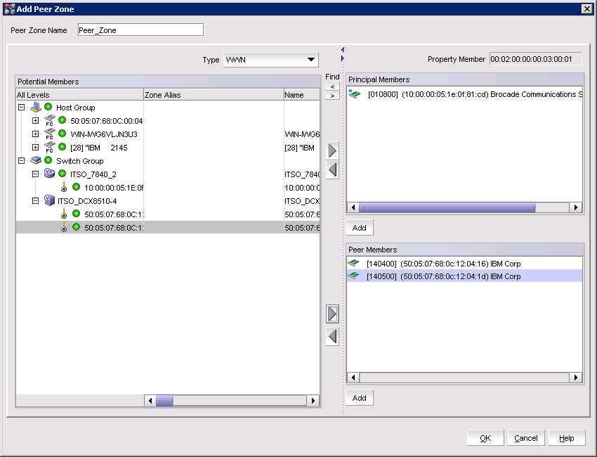
Figure 10-8 Add Peer Zone window
10.6 Trunking
Trunking optimizes the use of bandwidth by allowing a group of links to merge into a single logical link, called a trunk group. Traffic is distributed dynamically and in order over this trunk group, achieving greater performance with fewer links. Within the trunk group, multiple physical ports appear as a single port, thus simplifying management. Trunking also improves system reliability by maintaining in-order delivery of data and avoiding I/O retries if one link within the trunk group fails.
Trunking is frame-based instead of exchange-based. Because a frame is much smaller than an exchange, frame-based trunks are more granular and better balanced than exchange-based trunks and provide maximum utilization of links.
For information about trunking and trunking requirements, see Chapter 4, “IBM Network Advisor” on page 49.
10.6.1 Configuring trunk groups
After the Trunking license is installed, the ports that are to be used in trunk groups must be reinitialized (cycle the port through the offline state). This procedure needs to be performed only once, and is required for all types of trunking. Alternatively, the switch can be disabled and enabled.
Displaying trunking
Ports that are involved in trunking configurations can be displayed by using both IBM Network Advisor and the CLI.
To view trunk ports in CLI, complete the following steps:
1. Connect to the switch and log in using an account that is assigned to the admin role.
Example 10-1 shows trunking groups 1, 2, and 3; ports 4, 13, and 14 are masters.
switch:admin> trunkshow
1: 6-> 4 10:00:00:60:69:51:43:04 99 deskew 15 MASTER
2: 15-> 13 10:00:00:60:69:51:43:04 99 deskew 16 MASTER
12-> 12 10:00:00:60:69:51:43:04 99 deskew 15
14-> 14 10:00:00:60:69:51:43:04 99 deskew 17
13-> 15 10:00:00:60:69:51:43:04 99 deskew 16
3: 24-> 14 10:00:00:60:69:51:42:dd 2 deskew 15 MASTER
Ports that are involved in trunking configurations show in a number of areas of IBM Network Advisor. The easiest place to view trunking configurations is in the product view of the main IBM Network Advisor window.
To view the ports that are used in a trunk configuration, complete the following steps:
1. Open IBM Network Advisor and log in using an account assigned to the admin role.
2. Click the SAN tab to display the product list pane.
3. In the product pane list, click the + symbol to expand the port view for the selected switch.
4. Ports that are part of a trunk group will display as a trunk port, as shown in Figure 10-9.
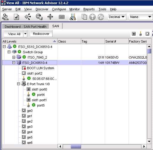
Figure 10-9 Product list pane
10.6.2 Enabling Trunking
Trunking can be enabled for a single port or for an entire switch. Trunking is automatically enabled when you install the Trunking license. The procedure is only required if trunking has been disabled on a port or switch. Enabling trunking disables and reenables the affected ports. As a result, traffic through these ports might be temporarily disrupted.
Complete the following steps to enable trunking with the CLI:
1. Connect to the switch and log in using an account assigned to the admin role.
2. Enter the portCfgTrunkPort command to enable trunking on a port. Enter the switchCfgTrunk command to enable trunking on all ports on the switch.
portcfgtrunkport[slot/]port mode
switchcfgtrunk mode
Mode 1 enables trunking. Example 10-2 shows trunking being enabled.
Example 10-2 Trunking is being enabled on slot 1, port 3.
switch:admin> portcfgtrunkport 1/3 1
To enable port trunking with IBM Network Advisor, complete the following steps:
1. Open IBM Network Advisor and log in using an account that is assigned to the admin role.
2. Select the SAN tab to display the Product list pane.
3. Right-click the switch that you want to enable trunking for, and select Element Manger → Ports. The Web Tools window is displayed with the FC Ports tab selected as shown in Figure 10-10 on page 267.
4. Change the window view to Advanced by selecting View and then Advanced to enable the required menu options for the following steps.
5. Highlight the port for which trunking is to be enabled in the FC Ports Explorer pane.
6. Click Actions and select Trunking → Enable. Ensure that trunking is enabled for that port.
Figure 10-10 shows the enable trunking option for a port.
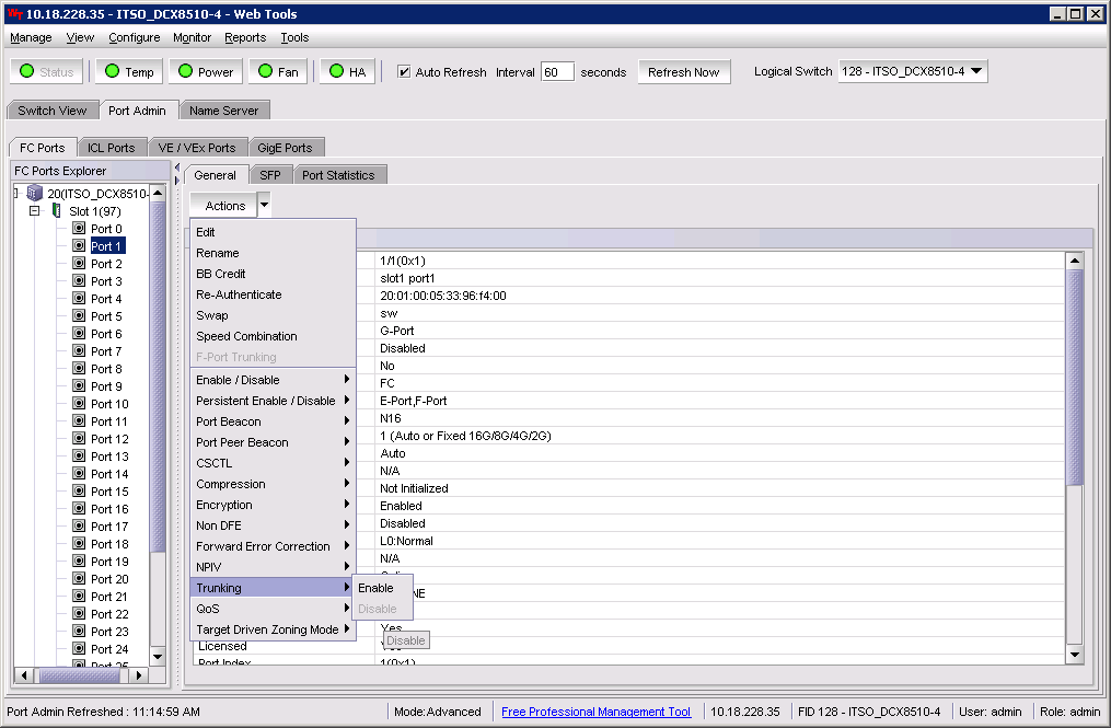
Figure 10-10 Enable the trunking option in Web Tools
10.6.3 Types of trunking
Trunking can be between two switches, between a switch and an Access Gateway module, or between a switch and a compatible adapter. The following configurations are possible:
•ISL trunking, or E_Port trunking, is configured on an inter-switch link (ISL) between two Fabric OS switches and is applicable only to E_Ports.
•ICL trunking is configured on an inter-chassis link (ICL) between two IBM System Networking SAN384B-2 (2499-416) and IBM System Networking SAN768B-2 (2499-816) and is applicable only to ports on the core blades.
•EX_Port trunking is configured on an inter-fabric link (IFL) between an FC router (EX_Port) and an edge fabric (E_Port). The trunk ports are EX_Ports connected to E_Ports.
•F_Port trunking is configured on a link between a switch and either an Access Gateway module or a Brocade adapter. The trunk ports are F_Ports (on the switch) connected to N_Ports (on the Access Gateway or adapter).
•N_Port trunking is configured on a link between a switch and either an Access Gateway module or a compatible adapter. It is similar to F_Port trunking. The trunk ports are N_Ports (on the Access Gateway or adapter) connected to F_Ports (on the switch).
ISL trunking is the typical use case. Detailed information is available in the Fabric OS Administrators Guide, which is available at the following website:
10.7 Fibre Channel over distance
When you need fabric connectivity over longer distances, SANs are typically connected over metro or long-distance networks. In both cases, path latency is critical for mirroring and replication solutions. For native Fibre Channel links, the amount of time that a frame spends on the cable between two ports is negligible because that aspect of the connection speed is limited only by the speed of light. The speed of light in optics amounts to approximately 5 microseconds per kilometer, which is negligible compared to the typical disk latency of 5 - 10 milliseconds. The Extended Fabrics feature enables full-bandwidth performance across distances spanning up to hundreds of kilometers. It extends the distance ISLs can reach over an extended fiber by providing enough buffer credits on each side of the link to compensate for latency that is introduced by the extended distance.
10.7.1 Buffer credits
Buffer credits are a measure of frame counts, and are not dependent on the data size (a 64-byte and a 2-KB frame both consume a single buffer). Consider the following parameters when allocating buffers for long-distance links that are connected through dark fiber or through a D/CWDM in a pass-through mode:
•Round Trip Time (RTT) (that is, the distance)
•Frame processing time
•Frame transmission time
Below are some suggested guidelines for calculating the number of required buffer credits:
•Number of credits = 6 + ((link speed Gbps * Distance in KM) / frame size in KB).
Example: 100 KM @2k frame size = 6 + ((8 Gbps * 100) / 2) = 406
•A buffer model should be based on the average frame size.
•If compression is used, the number of buffer credits that is needed is 2x the number of credits without compression.
On the IBM b-type 16 Gbps backbones platform, 4 K buffers are available per ASIC to drive the 16 Gbps line rate to 500 KM at a 2 KB frame size. Additional control is available when LD or LS links are configured. Using these links allows the number of required buffer credits to be specified based on the anticipated or real average frame size for a long-distance port. Using the frame size option, the number of buffer credits that are required for a port is automatically calculated. These options give extra flexibility to optimize performance on long-distance links.
In addition, FOS 7.1 and later provides commands to gain better insight into long-distance link traffic patterns by displaying the average buffer usage and average frame size through the CLI.
The portBufferCalc command can automatically calculate the number of buffers that are required per port given the distance, speed, and frame size. The number of buffers that is calculated by this command can be used when configuring long-distance ports.
|
Note: If no options are specified, then the current port’s configuration is used to calculate the number of buffers that are required.
|
10.7.2 Fabric interconnectivity over Fibre Channel at longer distances
SANs spanning data centers in different physical locations can be connected through dark fiber connections by using Extended Fabrics with wave division multiplexing, such as dense wavelength division multiplexing (DWDM), coarse division multiplexing (CWDM), and time-division multiplexing (TDM). Extended Fabrics is a FOS optionally licensed feature This situation is similar to connecting switches in the data center with one exception: Additional buffers are allocated to E_Ports connecting over distance. The Extended Fabrics feature extends the distance that the ISLs can reach over an extended fiber. This task is accomplished by providing enough buffer credits on each side of the link to compensate for the latency that is introduced by the extended distance.
Any of the first eight ports on the 16 Gbps port blade can be set to 10 Gbps FC for connecting to a 10 Gbps line card D/CWDM without needing a specialty line card. If you connect to DWDMs in a pass-through mode where the switch is providing all the buffering, a 16 Gbps line rate can be used for higher performance.
Extended Fabrics device limitations
It is suggested that FC8-64 and FC16-64 port blades not be used for long distance because of their limited buffers. These blades do not support long-wavelength (LWL) fiber optics and therefore only support limited distance. However, the ports can still be configured to reserve frame buffers for the ports that are intended to be used in long-distance mode through DWDM.
|
Note: A limited number of reserved buffers can be used for long distance for each blade. If some ports are configured in long-distance mode and have buffers reserved for them, insufficient buffers might remain for the other ports. In this case, some of the remaining ports might come up in degraded mode.
|
10.8 Fibre Channel over IP
FCIP enables you to use the existing IP wide area network (WAN) infrastructure to connect Fibre Channel SANs.
The TCP connections ensure in-order delivery of Fibre Channel (FC) frames and lossless transmission. The Fibre Channel fabric and all Fibre Channel targets and initiators are unaware of the presence of the IP WAN.
The advantage of this configuration is that the existing, less expensive IP WAN network can be used to encapsulate and transmit the Fibre Channel frame over long distances while still ensuring the high integrity required for storage I/O.
Figure 10-11 shows the Fibre Channel frame being encapsulated and decapsulated for transport across the WAN.
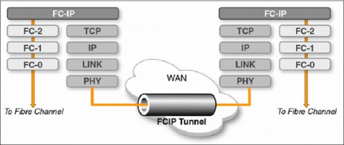
Figure 10-11 FCIP encapsulation
The extension switch or blade accomplishes the FCIP connection by establishing a tunnel that emulates FC ports on each end of the tunnel.
When the tunnel is configured and the connection is established between the devices, a circuit is formed. Either an ISL or an IFL can be created depending on the configuration that you want.
When the circuit is formed and functioning, the virtual FC that is created can be configured as a Virtual E port (VE-Port) or an FCR connection, a Virtual Extended port (VEX-port) to link the two ends.
Figure 10-12 shows the tunnel and circuit concept.

Figure 10-12 Tunnel and circuits concept
10.8.1 Configuring an FCIP tunnel
The detailed steps for FCIP tunnel configuration are provided in the Fabric OS FCIP Administrator’s Guide that you can download at the following website:
The following is the general outline of those steps:
1. Persistently disable VE_Ports.
2. If required, configure VEX_Ports. For more information, see 10.10, “FCIP and FCR” on page 274.
3. Set the media type or operating mode.
4. Create an IP interface (IPIF) for each circuit that you want on a port by assigning an IP address, netmask, and an IP maximum transfer unit (MTU) size to an Ethernet port.
5. Create one or more IP routes to a port.
6. Test the IP connection.
7. Create the FCIP tunnel or tunnels.
|
Note: Configuring a tunnel automatically configures circuit 0 for the tunnel.
|
8. Persistently enable the VE_Ports.
10.9 FC-FC routing overview
Fibre Channel routing allows two or more FC devices to communicate across fabrics without requiring them to merge.
For routing to take place, there must be either a router or routing blade, or the switch must have the capability to perform integrated routing.
The integrated routing license allows ports in supported switches to be configured as EX_Ports or VEX_Ports supporting Fibre Channel Routing. This configuration eliminates the need to add a routing blade or the need for an external router for Fibre Channel Routing (FCR) purposes.
Routing is accomplished by creating virtual domains in the remote switch to facilitate traffic flow into and out of the individual fabrics. The virtual domains are known as translate (XD) or front (FD) domains, depending on where they are:
•The XD domain is in the switch or blade that is responsible for routing between fabrics.
•The FD domain is projected into the remote fabric.
See Figure 10-13 for an example.
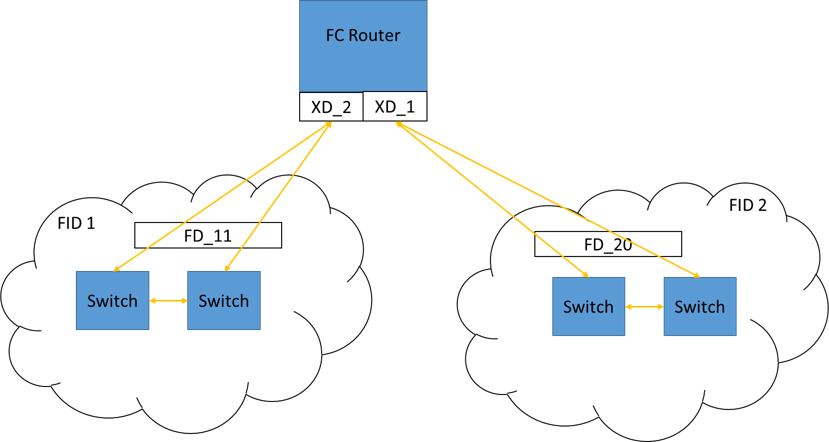
Figure 10-13 Routing concept
Using FC-FC routing, you can share resources across multiple fabrics without the administrative problems, such as change management, network management, scalability, reliability, availability, and serviceability, that might result from merging the fabrics.
A Fibre Channel router (FC router) is a switch that is running the FC-FC routing service. The FC-FC routing service can be simultaneously used as an FC router and as a SAN extension over WANs by using FCIP.
10.9.1 Setting up FC to FC routing
Complete the following tasks to set up and configure FC to FC routing:
1. Verify that you have the proper setup for FC to FC routing.
2. Assign backbone fabric IDs.
3. Configure FCIP tunnels if you are connecting Fibre Channel SANs over IP-based networks.
4. Configure IFLs for edge and backbone fabric connection.
5. Modify port cost for EX_Ports, if you want to change from the default settings.
6. Enable shortest IFL mode if you want to choose a lowest cost IFL path in the backbone fabric.
7. Configure trunking on EX_Ports that are connected to the same edge fabric.
8. Configure Logical SAN (LSAN) zones to enable communication between devices in different fabrics.
The detailed commands for each step are documented in the Fabric OS Administrator’s Guide at the following link:
10.9.2 Logical SAN Zones
An LSAN consists of zones in two or more edge or backbone fabrics that contain the same devices. LSANs essentially provide selective device connectivity between fabrics without requiring the fabrics to merge.
|
Note: A backbone fabric consists of one or more FC switches with configured EX_Ports. These EX_Ports in the backbone connect to edge fabric switches through E_Ports. This type of EX_Port-to-E_Port connectivity is called an IFL.
|
To enable device sharing across multiple fabrics, LSAN zones must be created on the edge fabrics. and optionally on the backbone fabric as well. Use normal zoning operations to create zones (see 10.5, “Zoning” on page 260) with names that begin with the special prefix “LSAN_”, and adding host and target port WWNs from both local and remote fabrics to each local zone as wanted. Zones on the backbone and on multiple edge fabrics that share a common set of devices will be recognized as constituting a single multi-fabric LSAN zone. The devices that they have in common will then be able to communicate with each other across fabric boundaries.
SAN zone members in all fabrics must be identified by their WWN. You cannot use the port IDs that are supported only in Fabric OS fabrics.
|
Note: The name of an LSAN zone begins with the prefix “LSAN_”. The LSAN name is case-insensitive, so lsan_ is equivalent to LSAN_, Lsan_, and so on.
|
Peer LSAN zone support
Starting with Fabric OS 7.4.0, the FC router supports the peer LSAN zones if configured in the edge fabric. Peer zoning rules are applied by the edge fabric switch. The FC router treats peer LSAN zones as normal LSAN zones and imports the devices in the edge fabric as per a pair-matching algorithm. For more information, see 10.5.2, “Peer Zoning” on page 262.
10.9.3 Fibre Channel routing and virtual fabrics
If the Virtual Fabrics feature is enabled (see Chapter 8, “Virtual Fabrics” on page 213), then in the FC-FC routing context, a base switch is like a backbone switch and a base fabric is like a backbone fabric.
If Virtual Fabrics is enabled, the following rules apply:
•EX_Ports and VEX_Ports can be configured only on the base switch.
•When Virtual Fabrics are enabled, the chassis is automatically rebooted. When the switch comes up, only one default logical switch is present, with the default fabric ID (FID) of 128. All previously configured EX_Ports and VEX_Ports are persistently disabled with the reason that ExPort is a non-base switch. A base switch must be explicitly created and the EX_Ports and VEX_Ports moved to that base switch, before you can enable the ports.
•If EX_Ports or VEX_Ports are moved to any logical switch other than the base switch, these ports are automatically disabled.
•EX_Ports can connect to a logical switch that is in the same chassis or in a different chassis. However, the following configuration rules apply:
– If the logical switch is on the same chassis, the EX_Port FID must be set to a different value than the FID of the logical switch to which it is connecting.
– If the logical switch is on a different chassis, no FID for any logical switch in the FC router backbone fabric can be the same as the FID of the logical switch to which the EX_Port is connecting.
•If an EX_Port or VEX_Port is connected to an edge fabric, ensure that there are no logical switches with extended ISL (XISL) use enabled in that edge fabric. If any logical switch in the edge fabric allows XISL use, then the EX_Port or VEX_Port is disabled.
•Backbone-to-edge routing is not supported in the base switch.
•All FC router commands can be executed only in the base switch context.
•The fcrConfigure command is not allowed when Virtual Fabrics is enabled. Instead, use the lsCfg command to configure the FID.
•Although the IBM System Networking SAN48B-5 and IBM System Networking SAN96B-5 support up to four logical switches, if you are using FC-FC routing, they can have a maximum of only three logical switches.
10.10 FCIP and FCR
The FCIP tunnel traditionally traverses a WAN or IP cloud, which can have characteristics that adversely impact a Fibre Channel network. The FCIP link across a WAN is essentially an FC ISL over an IP link. In any design, it should be considered an FC ISL.
Repeated flapping of a WAN connection can cause disruption in directly connected fabrics. This disruption might come about from many fabric services trying to reconverge repeatedly. This situation causes the processor on the switch or director to go to full capacity.
If the processor can no longer process the various tasks that are required to operate a fabric, an outage might occur. If you limit the fabric services to within the local fabric itself and do not allow them to span across the WAN, you can prevent this situation from occurring.
FCR provides a termination point for fabric services, referred to as a demarcation point. EX_Ports and VEX_Ports are demarcation points in which fabric services are terminated, forming the “edge” of the fabric. A fabric that is isolated in such a way is referred to as an edge fabric. There is a special case in which the edge fabric includes the WAN link because a VEX_Port was used. This type of edge fabric is referred to as a remote edge fabric.
FCR does not need to be used unless a production fabric must be isolated from WAN outages. When connecting to array ports directly for Remote Data Replication (RDR), FCR provides no benefit. Mainframe environments are precluded from using FCR, as it is not supported by FICON.
When a mainframe host writes to a volume on the direct access storage device (DASD), and that DASD performs RDR to another DASD, then DASD to DASD traffic is not using FICON. It is using an open systems RDR application such as IBM Metro Mirror or Global Mirror. These open-system RDR applications can use FCR, even though the volumes they are replicating are written by the FICON host.
The following are some basic FCR architectures:
•No FCR or one large fabric: This type of architecture is used with mainframes and when the channel extenders are directly connected to the storage arrays.
•Edge-backbone-edge: Edge fabrics bookend a transit backbone between them.
•VEX_Port: When a VEX_Port is used, the resulting architecture can be either backbone-remote edge or edge-backbone-remote edge, depending on whether devices are connected directly to the backbone or an edge fabric hangs from the backbone. Both are possible.
10.10.1 Using EX_Ports and VEX_Ports
If an FCR architecture is indicated, an “X” port is needed. An “X” port is a generic reference for an EX_Port or a VEX_Port. The only difference between an EX_Port and a VEX_Port is that the “V” indicates that it is FCIP-facing. The same holds true for E_Ports and VE_Ports; VE_Ports are E_Ports that are FCIP-facing.
The preferred practice in an FC routed environment is to build an edge fabric to backbone to edge fabric (EBE) topology. This topology provides isolation of fabric services in both edge fabrics. This topology requires an EX_Port from the backbone to connect to an E_Port in the edge fabric, as shown in Figure 10-14. The backbone fabric continues to be exposed to faults in the WAN connections. However, because its scope is limited by the VE_Ports in each edge fabric, and because edge fabric services are not exposed to the backbone, it does not pose any risk of disruption to the edge fabrics in terms of overrunning the processors or causing a fabric service to become unavailable. The edge fabric services do not span the backbone. See Figure 10-14.
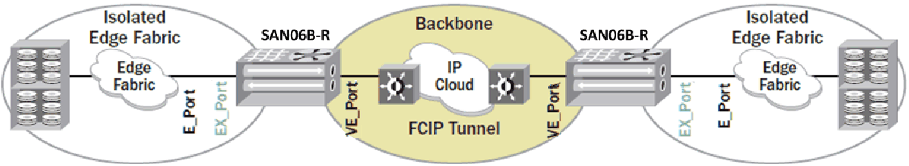
Figure 10-14 Edge-backbone-edge FCR architecture
There might be cases in which an EBE topology cannot be accommodated. Alternatively, the main production fabric can be isolated from aberrant WAN behavior while allowing the backup site to remain exposed. This topology provides a greater degree of availability and less risk compared to not using FCR at all. This topology uses VEX_Ports that connect to a remote edge fabric. The point is that the remote edge fabric continues to be connected to the WAN, and the fabric services span the WAN all the way to the EX_Port demarcation point. The fabric services that span the WAN are subject to disruption and repeated reconvergence, which can result in an outage within the remote edge fabric. This situation might not be of great concern if the remote edge fabric is not being used for production (merely for backup) because such WAN fluctuations are not ongoing.
You can build two topologies from remote edge fabrics. In the first, shown in Figure 10-15, production devices are attached directly to the backbone. In the second, shown in Figure 10-16 on page 276, the backbone connects to a local edge fabric. In both cases, the other side is connected to a remote edge fabric through a VEX_Port. Also in both cases, the production fabrics are isolated from the WAN. Between the two architectures, the second architecture with the edge fabric is preferred for higher scalability. The scalability of connecting devices directly to the backbone is relatively limited.
Figure 10-15 shows an example of Backbone-remote edge architecture
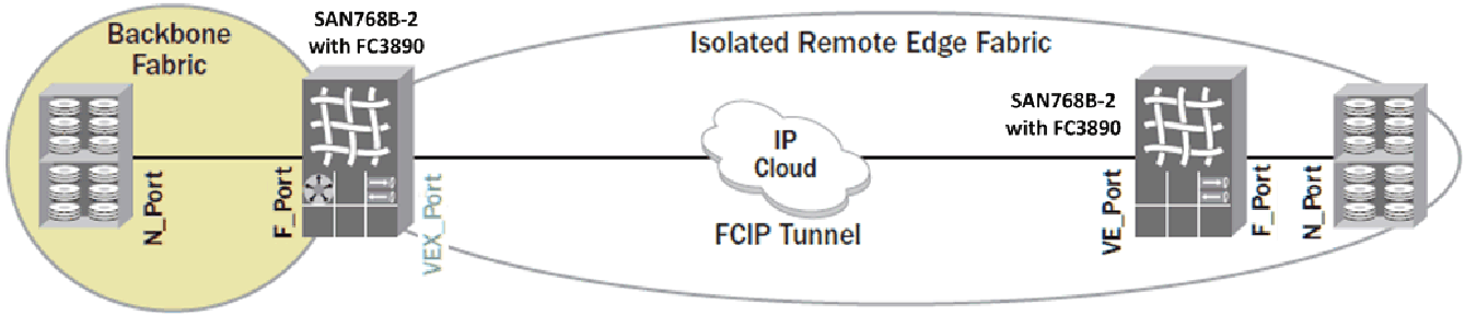
Figure 10-15 Backbone-remote edge architecture
Figure 10-16 shows an example of Edge-remote edge architecture.
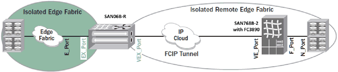
Figure 10-16 Edge-remote edge architecture
There are more considerations with “X” ports. When FC routing is configured, the path from initiator to target might pass through only one “X” port. Paths with more than one “X” port are not supported.
Figure 10-17 shows supported and unsupported paths through FC routing configurations.
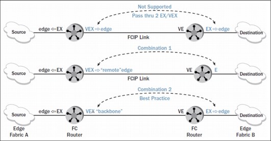
Figure 10-17 Supported and unsupported paths through FC routing configurations
The Integrated Routing (IR) license, which enables FCR on IBM b-type switches and directors, is needed only on the switches or directors that implement the “X” ports. Any switches or directors that connect to “X” ports and have no “X” ports of their own do not need the IR license. The IR license is not needed on the E_Port/VE_Port side to connect to the EX_Port/VEX_Port side.
|
Tip: VEX ports are not supported on the SAN42B-R. An alternative approach is to use VE to VE FCIP connections.
|
10.11 Access Gateway and N_Port ID Virtualization
One of the main limits to Fibre Channel scalability is the maximum number of domains (individual physical or virtual switches) in a fabric. Keeping the number of domains low reduces much of the impact that is typically attributed to SAN fabrics. Small-domain-count fabrics are more reliable, perform better, and are easier to manage. When configuring the edge switches in Access Gateway (NPV for Cisco or Transparent for Qlogic) mode, the mode eliminates the usage of a domain ID.
In an environment with multivendor edge switches, the N_Port ID Virtualization (NPIV) feature allows those switches to be presented in a transparent mode to the fabric, which reduces interoperability issues.
Figure 10-18 illustrates the difference between traditional E port connectivity and a switch that is configured to function as an access gateway.
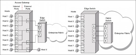
Figure 10-18 Differences between E port connectivity (right) and Access Gateway connectivity (left)
NPIV enables a single Fibre Channel protocol port to appear as multiple, distinct ports, providing separate port identification within the fabric for each operating system image behind the port. This configuration appears as though each operating system image had its own unique physical port. NPIV assigns a different virtual port ID to each Fibre Channel protocol device. NPIV enables you to allocate virtual addresses without affecting your existing hardware implementation. The virtual port has the same properties as an N_Port, and can register with all services of the fabric.
Each NPIV device has a unique device port ID (PID), Port WWN, and Node WWN, and behaves the same as all other physical devices in the fabric. Multiple virtual devices that are emulated by NPIV appear no different from regular devices that are connected to a non-NPIV port.
The same zoning rules apply to NPIV devices as non-NPIV devices. Zones can be defined by domain, port notation, by WWN zoning, or a combination of these. However, to perform zoning to the granularity of the virtual N_Port IDs, you must use WWN-based zoning.
If you are using domain port zoning for an NPIV port, and all the virtual PIDs that are associated with the port are included in the zone, then a port login (PLOGI) to a non-existent virtual PID is not blocked by the switch. Rather, it is delivered to the device that is attached to the NPIV port. In cases where the device cannot handle such unexpected PLOGIs, use WWN-based zoning.
|
Note: For more information, see the Fabric OS Administrator’s Guide or the Access Gateway Administrator's Guide, which you can find at the following website:
|
10.12 Inter-chassis links
ICLs are high-performance ports for interconnecting multiple backbones, enabling industry-leading scalability while preserving ports for server and storage connections. Optical UltraScale ICLs, based on Quad Small Form Factor Pluggable (QSFP) technology, connect the core routing blades of two backbone chassis. Each QSFP-based ICL port combines four 16 Gbps links, providing up to 64 Gbps of throughput within a single cable. It offers up to 32 QSFP ports in a Brocade DCX 8510-8 chassis or 16 QSFP ports in a Brocade DCX 8510-4 chassis, with up to 2 Tbps ICL bandwidth and support for up to 100 meters on universal optical cables. The optical form factor of the QSFP-based ICL technology offers several advantages over the copper-based ICL design in the original platforms.
The second generation increased the supported ICL cable distance from 2 meters to
50 meters. The 100-meter ICL is supported beginning in Fabric OS 7.1.0, when using 100-meter-capable QSFPs over OM4 cable only, providing greater architectural design flexibility.
50 meters. The 100-meter ICL is supported beginning in Fabric OS 7.1.0, when using 100-meter-capable QSFPs over OM4 cable only, providing greater architectural design flexibility.
|
Note: Before Fabric OS 7.3.0, all the FE ports and ICL ports used the same buffer credit model. In Fabric OS 7.3.0 and later, ICL ports support a 2 km distance. To support this distance, you must use specific QSFPs and allocate a greater number of buffer credits per port.
|
The combination of four cables into a single QSFP provides incredible flexibility for deploying various different topologies, including a 9-chassis full-mesh design with only a single hop between any two points within the fabric.
In addition to these significant advances in ICL technology, the ICL capability still provides dramatic reduction in the number of ISL cables that are required, a four to one reduction compared to traditional ISLs with the same amount of interconnect bandwidth. Because the QSFP-based ICL connections are on the core routing blades instead of consuming traditional ports on the port blades, up to 33% more FC ports are available for server and storage connectivity.
ICL Ports on Demand are licensed in increments of 16 ICL ports. Connecting five or more chassis through ICLs requires an Enterprise ICL license.
10.12.1 Supported topologies
Two network topologies are supported by SAN768B-2 and SAN384B-2 platforms and UltraScale ICLs: Core/edge and mesh. Both topologies deliver unprecedented scalability while reducing ISL cables.
10.12.2 QSFP-based ICL connection requirements
To connect multiple b-type chassis through ICLs, a minimum of four ICL ports (two on each core blade) must be connected between each chassis pair. With 32 ICL ports available on the SAN768B-2 (with both ICL POD licenses installed), this configuration supports ICL connectivity with up to eight other chassis and at least 256 Gbps of bandwidth to each connected 16 Gbps b-type backbones.
Figure 10-19 shows a diagram of the minimum connectivity between a pair of SAN768B-2 chassis. The physical location of ICL connections might be different from what is shown here, but there should be at least two connections per core blade.
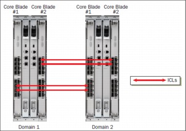
Figure 10-19 Minimum connections that are needed between a pair of SAN768B-2 chassis
The dual connections on each core blade must be within the same ICL trunk boundary on the core blades. ICL trunk boundaries are described in detail in 10.12.3, “ICL trunking and trunk groups” on page 280. If more than four ICL connections are required between a pair of SAN768B-2/SAN384B-2 chassis, add ICL connections in pairs (one on each core blade).
|
ICL connection preferred practice: Each core blade in a chassis must be connected to each of the two core blades in the destination chassis to achieve full redundancy. (For redundancy, use at least one pair of links between two core blades.)
|
A maximum of 16 ICL connections or ICL trunk groups between any pair of SAN768B-2/SAN384B-2 chassis is supported, unless they are deployed by using Virtual Fabrics, where a maximum of 16 ICL connections or trunks can be assigned to a single Logical Switch. This limitation is because of the maximum supported number of connections for FSPF routing. Effectively, there should never be more than 16 ICL connections or trunks between a pair of SAN768B-2/SAN384B-2 chassis, unless Virtual Fabrics is enabled and the ICLs are assigned to two or more Logical Switches. The exception to this rule is if eight port trunks are created between a pair of SAN768B-2/SAN384B-2 chassis, as described in 10.12.3, “ICL trunking and trunk groups”.
QSFP-based ICLs and traditional ISLs are not concurrently supported between a single pair of SAN768B-2/SAN384B-2 chassis. All inter-chassis connectivity between any pair of SAN768B-2/SAN384B-2 chassis must be done by using either ISLs or ICLs. The final layout and design of ICL interconnectivity is determined by the customer’s unique requirements and needs, which dictate the ideal number and placement of ICL connections between SAN768B-2/SAN384B-2 chassis.
10.12.3 ICL trunking and trunk groups
Trunking involves taking multiple physical connections between a chassis or switch pair and forming a single “virtual” connection, aggregating the bandwidth for traffic to traverse across. This section describes the trunking capability that is used with the QSFP-based ICL ports on the IBM b-type 16 Gbps chassis platforms. Trunking is enabled automatically for ICL ports, and cannot be disabled by the user.
Each QSFP-based ICL port has four independent 16 Gbps links, each of which terminates on one of four ASICs on each SAN768B-2 core blade, or two ASICs on each SAN384B-2 core blade. Trunk groups can be formed by using any of the ports that make up contiguous groups of eight links on each ASIC.
Figure 10-20 shows that each core blade has groups of eight ICL ports (indicated by the blue box around the groups of ports) that connect to common ASICs in such a way that their four links can participate in common trunk groups with links from the other ports in the group.
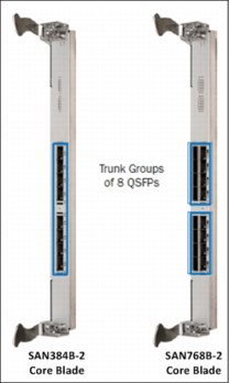
Figure 10-20 Core blade trunk groups
Each SAN384B-2 core blade has one group of eight ICL ports, and each SAN768B-2 core blade has two groups of eight ICL ports.
Because there are four separate links for each QSFP-based ICL connection, each of these ICL port groups can create up to four trunks, with up to eight links in each trunk.
A trunk can never be formed by links within the same QSFP ICL port because each of the four links within the ICL port terminates on a different ASIC for the SAN768B-2 core blade, or on either different ASICs or different trunk groups within the same ASIC for the SAN384B-2 core blade. Thus, each of the four links from an individual ICL is always part of independent trunk groups.
When connecting ICLs between a SAN768B-2 and a SAN384B-2, the maximum number of links in a single trunk group is four. This limitation is because the different number of ASICs on each product’s core blades, and the mapping of the ICL links to the ASIC trunk groups. To form trunks with up to eight links, ICL ports must be deployed within the trunk group boundaries that are shown in Figure 10-20. They can be created only when deploying ICLs between a pair of SAN768B-2 chassis or SAN384B-2 chassis. It is not possible to create trunks with more than four links when connecting ICLs between a SAN768B-2 and SAN384B-2 chassis.
As a preferred practice, deploy trunk groups in groups of up to four links by ensuring that the ICL ports that are intended to form trunks all are within the groups that are indicated by the red boxes in Figure 10-21.
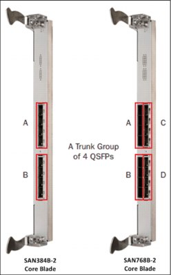
Figure 10-21 Core blade suggested trunk groups
Following this preferred practice, trunks can be easily formed by using ICL ports, whether two SAN768B-2 chassis are being connected, two SAN384B-2 chassis, or a SAN768B-2 and a SAN384B-2.
Any time that more ICL connections are added to a chassis, they should be added in pairs by including at least one additional ICL on each core blade. It is also a preferred practice that trunks on a core blade are always composed of equal numbers of links, and that connections be deployed in an identical fashion on both core blades within a chassis. As an example, if two ICLs are deployed within the group of four ICL ports in trunk group A in Figure 10-21, a single additional ICL can be added to trunk group A, or a pair of ICLs to any of the other trunk groups on the core blade. This configuration ensures that no trunks are formed that have a different total bandwidth from other trunks on the same blade. Deploying a single additional ICL to trunk group B might result in four trunks with 32 Gbps of capacity (those created from the ICLs in trunk group A) and four trunks with only 16 Gbps (those from the single ICL in group B).
The port mapping information that is shown in Figure 10-22 on page 282 and Figure 10-23 on page 283 also indicates the preferred ICL trunk groups by showing ports in the same preferred trunk group with the same color.
Core blade (CR16-8) port numbering layout
Figure 10-22 shows the layout of ports 0 - 15 on the SAN768B-2 CR16-8 line card. You can also see what the switchshow output would be if you ran a switchshow command within FOS by using the CLI.
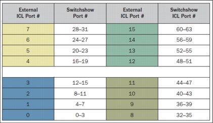
Figure 10-22 SAN768B-2 CR16-8 core blade - external ICL port numbering to “switchshow” (internal) port numbering
The colored groups of external ICL ports indicate those ports that belong to common preferred trunk groups. For example, ports 0 - 3 (shown in blue in Figure 10-22) form four trunk groups, with one link being added to each trunk group from each of the four external ICL ports. For the SAN768B-2, you can create up to 16 trunk groups on each of the two core blades.
The first ICL POD license enables ICL ports 0 - 7. Adding a second ICL POD license enables the remaining eight ICL ports, ports 8 - 15. This change applies to ports on both core blades.
|
Note: To disable ICL port 0, you must run portdisable on all four “internal” ports that are associated with that ICL port.
|
Core blade (CR16-4) port numbering layout
Figure 10-23 shows the layout of ports 0 - 7 on the SAN384B-2 CR16-4 line card. You can also see what the switchshow output would be if you ran switchshow within FOS by using the CLI.
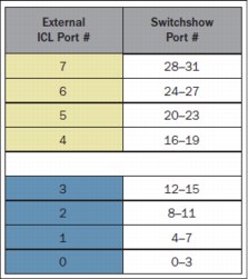
Figure 10-23 SAN384B-2 core blade - external ICL port numbering to “switchshow” (internal) port numbering
The colored groups of external ICL ports indicate those ports that belong to a common preferred trunk group. For example, ports 0 - 3 (shown in blue in Figure 10-23) form four trunk groups, with one link being added to each trunk group from each of the four external ICL ports. For the SAN384B-2, you can create up to eight trunk groups on each of the two core blades.
A single ICL POD license enables all eight ICL ports on the SAN384B-2 core blades. This change applies to ports on both core blades.
|
Note: To disable ICL port 0, you must run portdisable on all four “internal” ports that are associated with that ICL port.
|
10.12.4 ICL diagnostic tests
FOS V7.4.1 provides Diagnostic Port (D_Port) support for ICLs, helping administrators quickly identify and isolate ICL optics and cable problems. The D_Port on ICLs measures link distance and performs link traffic tests. It skips the electrical loopback and optical loopback tests because the QSFP does not support those functions. In addition, FOS V7.1 offers D_Port test CLI enhancements for increased flexibility and control.
10.12.5 Summary
The QSFP-based optical ICLs enable simpler, flatter, low-latency chassis topologies, spanning up to a 100-meter distance with standard cables. These ICLs reduce inter-switch cabling requirements and provide up to 33% more front-end ports for servers and storage, providing more usable ports in a smaller footprint with no loss in connectivity.
10.13 Fabric OS management
Fabric OS can be downloaded to a Backbone, which is a chassis, and to a non-chassis-based system, also referred to as a fixed-port switch. The difference in the download process is that Backbones have two Control Processors (CPs) and fixed-port switches have one CP. Both IBM Network Advisor and THE CLI can be used to upgrade or downgrade Fabric OS from either an FTP or SSH server by using FTP, SFTP, or SCP to the switch. Or, you can use a Brocade-branded USB device. IBM Network Advisor also offers a built-in FTP server.
|
Note: For detailed Firmware Management options including CLI-based instructions, see the Fabric OS Administers Guide available at the following website:
|
Not every release of FOS is certified for use on IBM branded switches. It is important to ensure that the level is listed in the IBM Support Portal for the switch platform.
All upgrades require, at minimum, that the release notes for the Fabric OS level be reviewed. However, you might also need to the Fabric OS Administrator Guide and the IBM Hardware Installation, Service and User Guide for the platform that is being upgraded or rolled back depending on your familiarity with the hardware. All these items are available through the IBM support portal link.
All code is obtained by using the IBM support portal. However, this portal redirects to the Brocade IBM assist website to download the code.
The IBM support portal is available at the following link:
New firmware consists of multiple files in the form of RPM packages listed in a .plist file. The .plist file contains specific firmware information (time stamp, platform code, version, and so on) and the names of packages of the firmware to be downloaded. These packages are made available periodically to add features or to remedy defects. Contact your switch support provider to obtain information about available firmware versions.
All systems maintain two partitions (a primary and a secondary) of nonvolatile storage areas to store firmware images. The firmware download process always loads the new image into the secondary partition. It then swaps the secondary partition to be the primary and high availability (HA) reboots the system (which is nondisruptive). After the system boots up, the new firmware is activated. The firmware download process then copies the new image from the primary partition to the secondary partition.
In dual-CP systems, the firmware download process, by default, sequentially upgrades the firmware image on both CPs using HA failover to prevent disruption to traffic flowing through the Backbone. This operation depends on the HA status on the Backbone.
For an IBM System Storage SAN384B-2 and SAN768B-2 Backbone family product, with one or more AP blades, Fabric OS automatically detects mismatches between the active CP firmware and the blade’s firmware, and triggers the auto leveling process. This auto-leveling process automatically updates the blade firmware to match the active CP. At the end of the auto-leveling process, the active CP and the blade run the same version of the firmware.
Since version 6.0.0, a one level nondisruptive upgrade is supported. Therefore, to go from 7.0.x to 7.4.x, the path would require multiple updates, if the intent is to do so non-disruptively. The suggested practice is to use the last release in each major release level. The example above would require an update path consisting of 7.1.x → 7.2.x → 7.3.x → 7.4.x where “x” is a sub release within the major release of that level.
10.13.1 Firmware download enhancements
FOS v7.4 introduces the following enhancements for firmware download:
•Staged Firmware Download
FOS v7.4 supports staged firmware download so that users can download firmware package to a switch first and choose to install and activate the downloaded firmware later.
•Firmware Clean Installation
FOS v7.4 supports firmware clean installation, which installs a firmware package without retaining the existing configuration or maintaining HA. With this feature, customers receiving a new switch from the factory can install firmware in a single step to the wanted version that their networks are running, without going through multiple steps of nondisruptive firmware download.
•Firmware Auto Sync Enhancement
FOS v7.4 enhances the firmware auto sync feature to support automatic synchronization of firmware versions on a standby CP with a version different from the active CP. If an active CP runs FOS v7.4 or higher, automatic upgrades and downgrades can be done in these circumstances:
– A standby CP with firmware version as early as FOS v6.4 can be upgraded automatically.
– A standby CP with firmware version later than FOS v7.4 can be downgraded automatically.
|
Note: For each switch in the fabric to be updated, complete all firmware download changes on the current switch before starting the upgrade or downgrade on the next switch. This process avoids disruption of traffic between switches in your fabric.
|
10.14 Upgrading firmware or rolling back to an earlier version
In most cases, firmware will be upgraded, which is installing a newer firmware version than the one currently running. However, some circumstances might require installing an older version, which is rolling back the firmware. The procedures in this section assume that firmware is being upgraded, but they also work for rolling back to an earlier version when the old and new firmware versions are compatible. Always reference the latest release notes for updates that might exist regarding rollbacks under particular circumstances.
|
Considerations for FICON Control Unit Port (CUP) environments: To prevent channel errors during nondisruptive firmware installation, the switch CUP port must be taken offline from all host systems.
|
10.14.1 Preparing for upgrades
Before you run a firmware upgrade, complete the tasks in this section. In the unlikely event of a failure or timeout, these preparatory tasks enable you to provide your switch support provider the information that is required to troubleshoot the firmware download.
1. Download the wanted Fabric OS package and the corresponding md5 sum file from the support portal at the following website:
2. Read the release notes for the new firmware to find out whether there are any updates related to the firmware download process.
3. Connect to the switch and log in using an account with admin permissions and verify the current version of Fabric OS and HA status. To confirm Fabric OS level and confirm HA status in IBM Network Advisor, complete the following steps:
a. In IBM Network Advisor, right-click the switch in the product or topology panes of the SAN tab and select Element Manager → Hardware to display the Hardware window in Web Tools (see Figure 10-24).
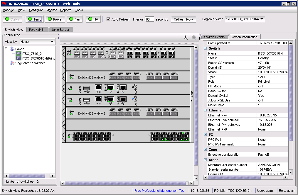
Figure 10-24 Web Tools Hardware window
b. Select the Switch information tab in the right pane to display the switch hardware information, including the Fabric OS version.
c. Click the HA button at the top of the panel to display the High Availability status window. If the status is not HA enabled, Heartbeat Up, HA State synchronized, you will need to troubleshoot the problem before the firmware upgrade can proceed.
Figure 10-25 shows the High Availability window.
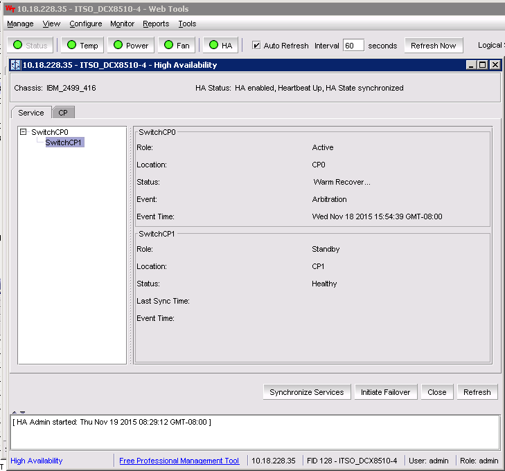
Figure 10-25 Web Tools High Availability window
4. Collect and save a switch configuration file on your FTP or SSH server, or USB memory device on supported platforms.
For information about collecting the switch configuration, see 4.12, “Scheduling daily or weekly backups for the fabric configuration” on page 101.
5. Connect to the switch and log in using an account with admin permissions. Collect and save a current supportsave before you run the Fabric OS upgrade. This information helps to troubleshoot the firmware download process if a problem is encountered.
For instructions for collecting a supportsave, see 12.7, “Collecting support data” on page 314.
10.14.2 Staging the Fabric OS package for download to the switch
After the Fabric OS version package has been downloaded locally to the Host running the IBM Network Advisor server, it must be added to the Firmware repository.
The firmware repository is used by the internal FTP, SCP, or SFTP server that is delivered with the Management application software. It can be used by an external FTP server if it is installed on the same platform as the Management application software. The repository is not available to FTP servers on external platforms.
To add a Fabric OS package to the firmware repository, complete the following steps:
1. Log in to IBM Network Advisor using an ID with admin privileges.
2. Select Configure → Firmware Management and the Firmware Management window will be displayed. Figure 10-26 shows the Firmware Management window with the Repository tab selected.
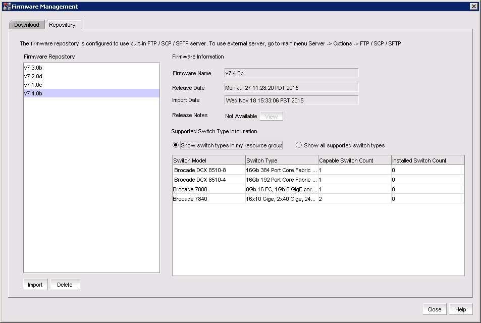
Figure 10-26 Firmware Management panel with the Repository tab selected
3. Select the Repository tab.
The right pane displays the current Fabric OS packages that are available in the repository. The left pane displays supported switches.
|
Note: In the Supported Switches pane, the show supported switches in my resource group or show supported switches radio buttons can be selected. The show supported switches in my resource group button shows only switches in the inventory that is currently discovered that support the fabric OS package that is selected in the Firmware Repository pane. The show supported switches option will show all supported products that are available from IBM.
|
4. To import a downloaded Fabric OS package into the repository, click Import to display the Import Firmware File window.
Packages can also be deleted by selecting a package in the repository pane and clicking Delete (see Figure 10-27).
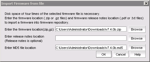
Figure 10-27 Import Firmware from File panel
5. Click Browse to browse to the downloaded Fabric OS package location on the local server and repeat the step for the md5 sum file.
6. Click OK to add the package to the repository. IBM Network Advisor confirms the file’s integrity by using the md5 file, and then extract and stage the file in the repository.
An Import completed successfully window will be displayed when complete.
7. Click OK to close the notification and the Firmware Repository window is displayed.
8. Click Close to close the Firmware Management window.
10.14.3 Upgrading firmware
To complete a Fabric OS upgrade with IBM Network Advisor, complete the following steps:
1. Log in to IBM Network Advisor using an ID with Admin privileges.
2. Select Configure → Firmware Management to display the Firmware Management window.
3. Select the Download tab.
The left pane displays switches that are available for firmware update, the right pane displays selected switches, and the lower right pane displays firmware update status details when a firmware update is underway (see Figure 10-28).
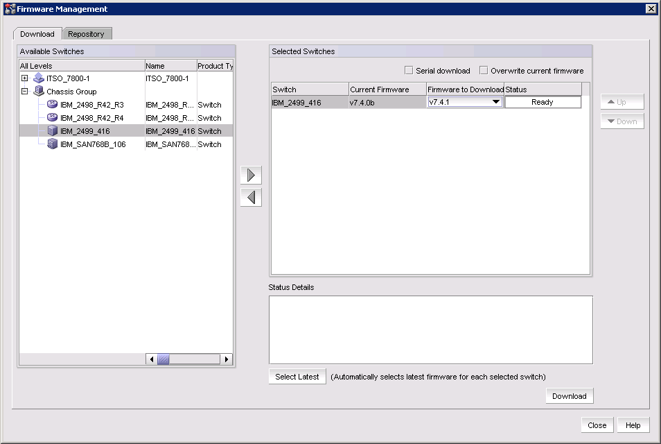
Figure 10-28 Firmware Download window with the Download tab selected
4. Select one or more switches from the Available Switches pane.
5. Click the right arrow to move the switches to the Selected Switches pane.
6. Select a specific version from the Firmware to Download column, or use Select Latest to automatically select the latest version.
7. To download the firmware to the selected switches one at a time, select Serial download.
– Use the Up and Down buttons to determine the order in which the firmware is downloaded to the switches. If firmware download fails on one switch, all other switches in the queue will be skipped.
– If the Serial download check box is cleared, the download occurs in parallel on the switches (up to 20 at a time).
8. To overwrite the current firmware, even if the selected version is the same as the version currently running on the switch, select Overwrite current firmware.
– While the firmware is downloaded to the device, the Status column displays the current download status. After the firmware download is complete, the Message column displays whether the download was a success or failure.
..................Content has been hidden....................
You can't read the all page of ebook, please click here login for view all page.