Transfer function
3.1.1 Instrumentation
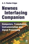
Instrumentation is concerned with producing a measurable output from the signal provided by a transducer. This is usually done through a series of steps or processes, starting with the transducer signal or input, Qi.
It is desirable to have linear relationships between the inputs and outputs of the various processes so that Q3 = K1 K2 K3 Qi.
In practice, errors and noise are transmitted at each step along with the signal of interest. The process of instrumentation is to maximise the transmission of signal and to minimise the errors and noise. The process is concerned with:
• the electrical nature of signals and methods of measurement
• signal processing by the application of a transfer function to provide amplification and filtering
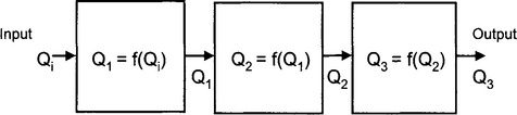
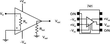
An important issue in connecting a transducer to a preamplifier is to ensure that maximum signal is transferred by a process called impedance matching.
Ideally, Rin ![]() Rs because otherwise, negligible ΔVin appears at the amplifier. That is, if RS
Rs because otherwise, negligible ΔVin appears at the amplifier. That is, if RS ![]() Rin, then most of the voltage variations ΔVS appear across Rs and not at the amplifier input. Amplifiers should have a high input impedance Rin compared to Rs, the output resistance of the source.
Rin, then most of the voltage variations ΔVS appear across Rs and not at the amplifier input. Amplifiers should have a high input impedance Rin compared to Rs, the output resistance of the source.
3.1.2 Transfer function
There is a definite relationship between the input signal S(t) and output response R(t) of an electronic circuit. The relationship is called the transfer function.
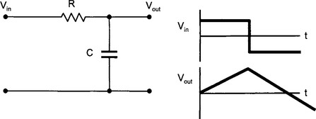
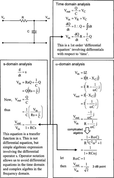
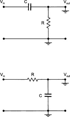
The transfer function is the ratio of the output voltage over the input voltage. This is a general definition and includes any phase effects that might be present in the circuit. For example, for the simple RC low pass filter shown below, the transfer function is:
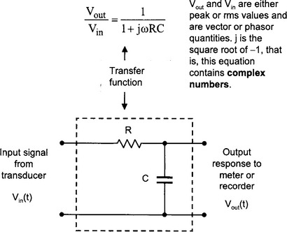
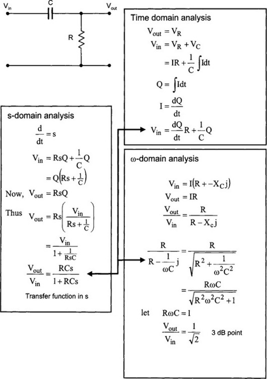
Later, we shall see how the transfer function for a wide variety of circuits (mainly filter circuits) can be obtained easily using operator notation. The transfer function for a particular filter circuit can be used to modify the signal being measured so as to eliminate noise (i.e. unwanted information). The mathematical representation of the transfer function allows the effect of various filter and amplifier circuits to be analysed and designed before any actual circuit is constructed.
3.1.3 Transforms
Many physical phenomena can be described by differential equations, that is, equations which involve derivatives. A short-hand way of writing ‘the derivative with respect to’ is to use the differential operator. For example:
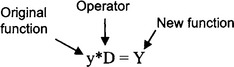
Here, D is a differential operator which, when applied to a function y(x), yields a new function in x. The differential operator may be quite complex, involving derivatives of higher orders. For example:
are constants thus
After the operator has been applied to the original function, a new function is formed. That is, the original function has been transformed into another function.
The differential operator is very useful for the treatment of many types of differential equations. Another type of transform is the integral transform operator T which has the form:
Here, f is a function of t which is transformed by the operator T. K is a function of the variables s and t. The integration produces a new function of s only and is the integral transform of the original function f(t). The function K(s, t) can take many forms, and an especially interesting one is that defined by:
The resulting integral transform is called the Laplace transform L[f(t)] of the function f(t).
3.1.4 Laplace transform
If the function f is a function of t, then the Laplace transform is defined as:
The resulting integral, that is, L[f(t)], is a function of s only: L[f(t)] = F(s). F(s) is the Laplace transform of f(t). The symbol ‘L’ is the Laplace operator which acts on f(t) to give the transformed function F(s).
A particularly interesting case is when f(t) is a periodic function, say f(t) =sinωt:
The results are shown here without showing the working.
Why are Laplace transforms important to us? Because they allow differential equations to be solved using algebraic expressions involving operators. We’ll see how this works in a moment. For now, consider yet another interesting Laplace transform, that of L[1].
Well, the question now is, “What is s”? Answer: It depends on the problem being analysed. For sinusoidal signals, it is appropriate to let s = jω.
Why bother with transforms? A particular input signal in the time domain may be transformed into another signal, or function, in the frequency domain. The transformed signal may then be operated upon by a filter and then transformed back into the time domain for display. The transform of a signal gives information about the composition of the signal.
3.1.5 Operator notation
Consider an integrator circuit:
It can be shown that the output voltage is the time integral of the input voltage:
when RC is large.
If the input signal is a sine wave, then the output signal is a cosine wave (whose amplitude decreases with increasing frequency of the input signal). It can be shown (see page 218) that the amplitude and phase relationship between Vin and Vout has the form (in complex number notation):
When RC is large, then:![]()
Let
and
‘s’ is an operator. In this case, a “differential” operator since the application of s to a function takes the time derivative of that function.
Thus,It appears therefore that in this application, s = jω.
Similarly for a differentiator,
and it can be shown:
when RC is small.

3.1.6 Differential operator
Now, if s = jω, and s also is a differential operator, then exactly what is ‘s’ ?

That is, ‘s’ is a differential operator for this function. Thus:
That is, in the Laplace transform, where K(s, t) = e−st, s can be considered a differential operator and not just an ordinary everyday variable.
For sinusoidal periodic functions, we can let s = jω and still have s act like a differential operator. Thus, the s-domain analysis allows us to carry frequency and phase information (for frequency domain analysis) or differential time information (for time domain analysis) in our calculations.
To analyse a circuit, the circuit is transformed into the s-domain, and the necessary algebra performed (which is usually more manageable) and the results transformed back into the frequency or time domain as required.
On the previous page, we saw how this dual nature of s was consistent with the response of a passive integrator. Let us now apply the technique again to the passive integrator and also the passive differentiator.
3.1.8 Differentiator – passive
It appears that s = jω is consistent with an ordinary complex number analysis of the two circuits. Next we will see the ‘s’ notation used in the analysis of active filter circuits.
3.1.9 Transfer impedance
The transfer impedance of a network is defined as the ratio of the voltage applied to the input terminals to the current which flows at the output terminals when the output is grounded.
3.1.10 Review questions
3.1.11 Activities
1. Connect a 741 op-amp to an appropriate power supply and connect the non-inverting input to ground and the inverting input to a variable DC voltage source. Describe what happens at the output when the input voltage is swept from −1 V to +1 V.
2. Sweep the voltage again slowly and determine the input voltage (to within a millivolt) when the output voltage is zero – you may have to modify the circuit slightly to obtain the best estimation of this crossover voltage.
3. With the non-inverting input still grounded, apply a small AC signal to the inverting input and measure the open-loop gain as a function of frequency. Record your readings in a table, and then plot gain in dB against log of frequency.
4. Determine the open-loop bandwidth of the op-amp.
5. Construct a simple inverting amplifier with a gain of 100. Check the input offset voltage and connect a nulling circuit to eliminate any offset.
6. Check the voltage at the inverting input and comment on its value.
7. Measure the frequency response of the amplifier. Determine the bandwidth.
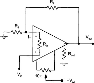
8. Measure the input resistance of the 741 IC by altering the circuit to a non-inverting amplifier configuration with a gain of 50.
9. Measure the output resistance by connecting a 100 Ω resistor to the output and to ground and determining the change from open circuit output voltage.
10. Alter the circuit to have a gain of 10 and measure the frequency response and input and output resistances. Compare with previously measured quantities and comment.
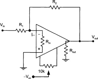
Offset null adjustment:Ground the input Vin. Turn the adjustment pot while observing Vout on an oscilloscope. A range of several volts each side of zero should be obtainable. Adjust the pot for zero on the output. 1μF capacitors may be connected between each power supply pin on the 741 to reduce RF pickup.
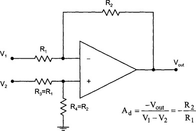
11. Construct a difference amplifier with a gain of 40.
12. Measure the frequency response and bandwidth of the amplifier.
13. Having measured the difference gain, devise a method to measure the common mode gain of the amplifier and then determine the common mode rejection ratio.
14. Measure the input resistance at each input and comment.