
13
Transact-SQL Programming Objects
SQL Server 2000 is an enormously capable relational data store. SQL Server 2005 is even more powerful. Both versions do a good job of storing large volumes of data. SQL Server in general manages transactions and enforces checks and rules to protect the integrity of related records and values. You've seen how the query optimizer makes intelligent decisions and uses indexes to make queries run fast and efficiently. Now we're going to take SQL Server to the next level. Most data is accessed through business applications. SQL Server can be more than just an idle medium for storing this data. A well-designed business solution uses the capabilities of an active database server, programming objects, and other components to distribute the workload and minimize unnecessary network traffic.
I want to take you on a brief tour of history so that you can appreciate the impact of the features we're about to discuss. In the 1980s and early 1990s, PC-based applications ran only on the desktop. If data could be shared across networks, it was simply stored in files managed by the file system. Applications supported a small number of users and quickly choked low-bandwidth networks as they moved all of their data to each desktop for processing. Desktop database applications sprang up like weeds in a new garden as inexpensive business applications became available—but the industry quickly hit the technology wall. In the past decade, the PC platform came of age with the advent of client/server database systems. In a nutshell, the enabling technology behind client/server applications was the cutting-edge concept of running application code on a database server. Products like SQL Server enabled this capability using database programming objects such as views and stored procedures.
I could stop there and keep things quite simple, but the current state of the industry has moved forward in recent years. Most enterprise database solutions have progressed beyond simple client/server technology. Now it's easier than ever before to distribute program components across two, three, or more different computers. These may include desktop computers, web servers, application servers, and database servers.
Sophisticated database applications use complicated queries. For this reason, it is important that queries and other SQL logic are protected and run as efficiently as possible. If SQL statements are managed in server-side database objects rather than in applications, this reduces the overall complexity of a solution. This separation of client-side applications and databases enables programmers and database professionals to each do what they do best, rather than having to write both program code and complex SQL, not to mention the fact that application programmers, unless they have a background in database technologies, have traditionally written very bad SQL.
The very first rule of developing database applications is to avoid the ad-hoc query at all costs. Ad-hoc queries create great efficiency issues, and when it comes to web applications, great security issues as well. The best practice when creating database-centric applications is to use database programming objects. In SQL Server, these objects include views, stored procedures, functions, and triggers. This chapter covers each of these objects in turn.
Views
This is one of the simplest database objects (at least views can be simple). On the surface, a view is nothing more than a SELECT query that is saved with a name in a database. Ask any modern-day programmer what they believe to be the most important and fundamental concept of programming. They will likely tell you that it is code reuse. Writing every line of code, every object, every script, and every query represents a cost or risk. One risk is that there could be a mistake (a bug) in the code. The cost of a bug is that it must be fixed (debugged) and tested. Buggy applications must be redeployed, shipped, installed, and supported. Undiscovered bugs pose a risk to productivity, business viability, and perhaps even legal exposure. One of the few constants in the software universe is change. Business rules will change, program logic will change, and the structure of your databases will also change. For all of these and other reasons, it just makes sense to reduce the number of objects that you create and use in your solutions. If you can create one object and reuse it in several places rather than duplicating the same effort, this limits your exposure to risk. Views promote this concept of code reuse by allowing you to save common queries into a uniform object. Rather than rewriting queries, complex queries can be created and tested and then reused without the added risk of starting over the next time you need to add functionality to an application.
Virtual Tables
One of the great challenges facing users is dealing with the complexity of large business databases. Many tools are available for use by casual database consumers for browsing data and building reports. Applications such as Microsoft Excel and Access are often used by information workers, rather than programmers, to obtain critical business management and operational information. A typical mid-scale database can contain scores of tables that contain supporting or special-purpose data. To reassemble the information stored in a large database, several tables must be joined in queries that take even skilled database professionals time and effort to create effectively. As you've seen in many examples, this is often not a trivial task. From the user's perspective, views are tables. They show up in most applications connecting to a SQL Server, along with the tables. A view is addressed in a SELECT statement and exposed columns, just like a table.
From the developer or database designer's perspective, a view can be a complex query that is exposed as if it were a simple table. This gives you an enormous amount of flexibility and the ability to hide all of the query logic, exposing a simple object. Users simply see a table-like object from which they can select data.
Creating a View
Defining a view is quite simple. First of all, a database user must be granted permission to create database objects. This is a task that you may want to have performed only by a database administrator or a select number of trusted users. Because creating most views isn't particularly complicated, you may want certain users to be granted this ability.
Several simplified tools are available that you can use to create views. Microsoft Access, Enterprise Manager, and Visual Studio all leverage the Transact-SQL Query Designer interface to create and manage views. The process is just about the same in all of these tools because they all actually expose the same components. The following section steps through creating a view using Microsoft Access. I will not demonstrate each tool because the process is nearly identical.
Creating a View in Microsoft Access
Microsoft Access is a popular tool that can be used to manage and query a SQL Server database. I don't intend for this example to serve as a full-blown Access tutorial so it's just going to demonstrate some of the basics. The following example is an Access Data Project (ADP) connected to the AdventureWorks2000 database.
In the database window shown in Figure 13-1, you can see that the database contains a stored procedure and two views, all listed on the Queries tab.
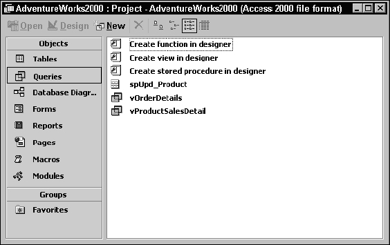
Figure 13-1
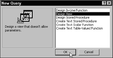
Click the New button on the toolbar to create a new query. The New Query window opens, allowing you to create a few different types of objects. Choose Design View, as shown in Figure 13-2, to create a new view and then click OK.
The next window should look familiar. Access uses a version of the Transact-SQL query designer window. In the default view, the table diagramming pane and the columns grid are displayed. The Access product designers made this tool appear as much as they could like the original Access SQL query designer by hiding the actual SQL script. The Add Table window, shown in Figure 13-3, is automatically opened. Use this to select and add three tables: Product, ProductCategory, and ProductSubCategory. Because of the relationships that exist between these tables, inner joins are automatically defined in the query.
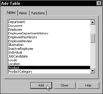
Figure 13-3
Select the Name column from the ProductCategory table (using the checkboxes in the table windows), the Name column from the ProductSubCategory table, and the columns you see in Figure 13-4, from the Product table. Using the Alias column in the columns grid, define aliases for the following three columns:
| Table.Column | Alias |
| ProductCategory.Name | CategoryName |
| ProductSubCategory.Name | SubCategoryName |
| Product.Name | ProductName |
Also, designate these three columns for sorting in the order listed by dropping down and selecting the word Ascending in the Sort Type column. Check your results against Figure 13-4 and make any adjustments necessary.
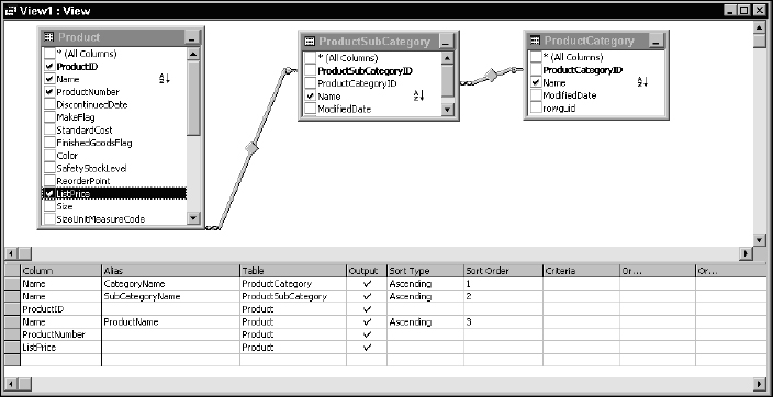
Figure 13-4
If you close the window, using the Close button in the top-right corner, Access will prompt you to save the view. Enter a name for the new view in the Save As dialog, as demonstrated in Figure 13-5. I've always made it a point to prefix view names with v, vw, or vw_ and to use Pascal-case (no spaces, with the first letter of each word capitalized).
Naming standards are discussed in more detail in Chapter 11. Just ensure that whatever you name your views is consistent and agreeable to those who will use it within your organization.
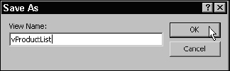
Figure 13-5
After saving the view, it appears in the list of objects on the Queries list. If you double-click the new item, it will open and display data just like a table, as you can see in Figure 13-6.
Creating Views in Visual Studio
All database objects are managed in the Server Explorer window. To create a view, it is first necessary to establish a connection to a SQL Server data source. After that, expand the connection and then right-click the node labeled Views. Select the New View menu item to launch the Transact-SQL Query Builder, as demonstrated in Figure 13-7.

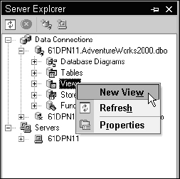
Figure 13-7
After the query is completed, close the Query Builder window. When prompted, provide a name for the new view.
When naming tables and other database objects it is important to consider the long-term implications. Keep in mind that individual views can be created to support a variety of application or reporting features. With so many views on the same entities, it becomes important to use unique, descriptive names.
Creating a View Using SQL Script
Regardless of the tool or product used to create a view, SQL script runs in the background and the result will be the same as handwriting without the use of an automated tool. The syntax for creating a new view is quite simple. The pattern is the same whether the query is very simple or extremely complex. I'll start with a simple view on a single table:
To continue working with this same view and extend its capabilities, I can either use the ALTER command to make modifications to the existing view or drop and create it. Using the ALTER statement rather than dropping and re-creating a view has the advantage of keeping any existing properties and security permissions intact.
Here are examples of these two statements. The ALTER statement is issued with the revised view definition:
ALTER VIEW vProductCosts
AS
SELECT ProductID, Name, ProductNumber, StandardCost
FROM Product
Using the DROP statement will wipe the slate clean, so to speak, reinitializing properties and security permissions:
DROP VIEW vProductCosts
What happens if there are dependencies on a view? I'll conduct a simple experiment by creating another view that selects data from the view previously created:
CREATE VIEW vProductCosts2
AS
Select Name, StandardCost From vProductCosts
For this view to work the first view has to exist and it must support the columns it references. Now, what happens if I try to drop the first view? I'll execute the previous DROP command. Here's what SQL Server returns:
Command(s) completed successfully.
My view is gone? What happens if I execute a query using the second view?
SELECT * FROM vProductCosts2
SQL Server returns this information:
Msg 208, Level 16, State 1, Procedure vProductCosts2, Line 1
Invalid object name ‘vProductCosts’.
Msg 4413, Level 16, State 1, Line 1
Could not use view or function ‘vProductCosts2’ because of binding errors.
Why would SQL Server allow me to do something so silly? I may not be able to answer this question to your satisfaction because I can't address the question to my own satisfaction. This ability to drop an object and break something else is actually documented as a feature call delayed resolution. It's actually a holdover from the early days of SQL Server. To a degree it makes some sense. The perk of this feature is that if you needed to write script to drop all of the objects in the database and then create them again, this would be difficult to pull off with a lot of complex dependencies. If you're uncomfortable with this explanation, there is good news. An optional directive on the CREATE VIEW statement called SCHEMA BINDING tells SQL Server to check for dependencies and disallow any modifications that would violate them. To demonstrate, the first thing I'll do is drop both of these views and then re-create them:
CREATE VIEW vProductCosts WITH SCHEMABINDING
AS
SELECT ProductID, Name, ProductNumber, StandardCost
FROM Product
GO

CREATE VIEW vProductCosts2 WITH SCHEMABINDING
AS
SELECT Name, StandardCost
FROM dbo.vProductCosts
Some unique requirements are apparent in the example script. First of all, for a view to be schema-bound, any objects it depends on must also be schema-bound. Tables inherently support schema binding, but views must be explicitly schema-bound.
Any dependent objects must exist in the database before they can be referenced. For this reason, it's necessary to use batch delineation statements between dependent CREATE object statements. This example used the GO statement to finalize creating the first view.
When referring to a dependent view, you must use a two-part name. This means that in SQL Server 2000, use the owner and object name (dbo, by default), and in SQL Server 2005, use the schema name (which, as you can see in this example, is also dbo). A schema-bound view also cannot use the SELECT * syntax. All columns must be explicitly referenced.
Ordering Rows
Back when the original ANSI SQL specification was written, the authors wanted to make sure that database designers wouldn't do dumb things in their SQL queries that would waste server resources. Keep in mind that this was at a time when production servers had 32MB of memory. One memory-intensive operation is reordering a large result set. So, in their infinite wisdom, the authors imposed a rule that views cannot support the ORDER BY clause unless the results are restricted using a Top Values statement.
I run into this restriction all of the time. I'll spend some time creating some big, multi-table join or sub-query with ordered results. After it's working, I think, “Hey, I ought to make this into a view.” So I slap a CREATE VIEW vMyBigGnarlyQuery AS statement on the front of the script and execute the script with this result:
The ORDER BY clause is invalid in views, inline functions, derived tables,
subqueries, and common table expressions, unless TOP or FOR XML is also specified.
Then I remember I have to use a TOP statement. This is a no-brainer and is easily rectified using the following workaround:
CREATE VIEW vProductCosts
AS
SELECT TOP 100 PERCENT ProductID, Name, ProductNumber, StandardCost
FROM Product
ORDER BY Name
Now that most database servers have 50 times the horsepower and 10 times the memory of those 10 to 15 years ago, ordering a large result set is of little concern.
Partitioned Views
Every system has its limits. Performance-tuning and capacity planning is the science of identifying these gaps and formulating appropriate plans to alleviate them. To partition data is to place tables or other objects in different files and on different disk drives to improve performance and organize data storage on a server. One of the most common methods to increase the performance and fault-tolerance of a database server is to implement RAID storage devices. I know this isn't a book on server configuration, but I bring this up for a good reason. In teaching classes on database design and talking about partitioning data across multiple hard disks, I've often heard experienced students ask, “Why don't you just use a RAID device? Doesn't this accomplish the same thing?” Yes, to a point, disk arrays using RAID 5 or RAID 10 simply spread data across an array of physical disks, improving performance and providing fault-tolerance. However, data partitioning techniques and using RAID are not necessarily mutually exclusive. Categorically, there may be three scenarios for server size and scale:
- Small-scale servers
- Medium-scale servers
- Large-scale servers
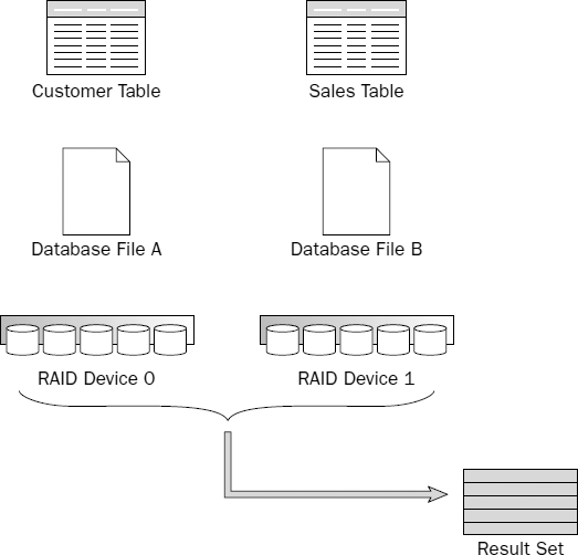
Small-scale servers will have system files and data on physical disks. You can implement data partitioning by placing objects in different database files residing on different disks, as depicted in Figure 13-8.
Moderate-scale servers may implement a RAID device where an array of identical physical disk drives is treated by the operating system as a single, logical volume. From the database designer's standpoint, the server has one disk, as illustrated in Figure 13-9. The fact that what we perceive to be a single hard disk drive is actually a bank of parallel disks is completely transparent and may have little impact on how we design our database. One could argue that there is no need to be concerned with partitioning because the RAID device does this for us — as long as we have ample disk space.
In a large-scale server environment, we generally take RAID technology for granted and may have several RAID devices, each acting as if it were an individual disk drive. This brings us back to the same scenario as the first example given where the server has a number of physical disks. In this case, we can partition our data across multiple disks, only each “disk” is actually a RAID device, as shown in Figure 13-10.
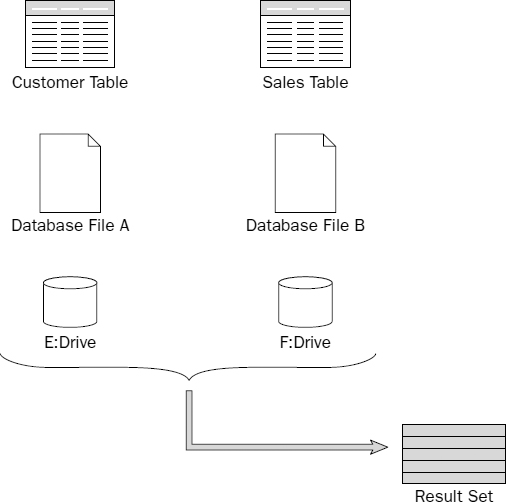
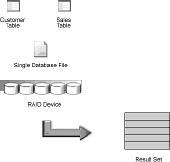
Figure 13-9
For this discussion, I'd like to put the RAID option aside and treat disks as if they are all physical disks, when in fact, each may be a RAID device.
So what does all of this have to do with views? You'll remember that one of the main reasons for views is to treat complex data as if it were a simple table. Partitioning takes this concept to the next level. Here's an example: Suppose that your product marketing business has been gathering sales order data for five years. Business has been good and, on average, you're storing 500,000 sales detail rows each year. At the end of each month your sales managers and executives would like to run comparative sales reports on all of this data but you certainly don't want to keep nearly three million rows of data in your active table. When database performance began to slow down a couple of years ago, you decided to archive older records by moving them to a different table. This improved transactional performance because the active sales detail table stored less data. As long as you only accessed the most current records for reporting, performance was fine. However, when you combined the archive tables with the current detail, you were back to where you started and, once again, the server ground to a snail's pace. This is because all of these tables resided on the same physical disk.
Here's a quick computer trivia question: What's the slowest component of almost any computer system? The user? OK, besides that. The memory? How about the CPU? Typically not. It's the hard disk. Aside from the cooling fans, the hard disk is the only critical component that is still mechanical. The industry hasn't yet found a cost-effective replacement without moving parts. The platter can only spin so fast and the read/write heads can only move back and forth so fast. In earlier chapters you learned that the greatest cost-affecting query performance is disk I/O—the time it takes for the system to position the heads and read data from a physical disk. If the system has one disk, it must find a page of data, reposition the heads, read the next page, and so on until it reads all of the data to return a complete result set. Because one disk has one set of heads, this happens in a linear fashion, one page at a time. If you were able to able to spread data across multiple disks, SQL Server could retrieve data from each disk simultaneously. The query execution plan makes this possible as it maps out those operations that are dependent and those that can be performed in parallel. This is depicted in Figure 13-11.
The view that makes all of this possible is actually quite simple. Using your successful marketing business as an example, the view definition might look like this:
SELECT * FROM SalesDetail_1999
UNION ALL
SELECT * FROM SalesDetail_2000
UNION ALL
SELECT * FROM SalesDetail_2001
UNION ALL
SELECT * FROM SalesDetail_2002
UNION ALL
SELECT * FROM SalesDetail_2004
UNION ALL
SELECT * FROM SalesDetail_Current
Because these tables are all addressable within the database, they can be referenced in joins, subqueries, or any type of SQL expression. It may not make sense to put every table on its own disk, but if you did, each of these SELECT statements could be processed in parallel. Assuming that each drive had its own independent controller, the data on each of these disks could be read simultaneously.
As you can see, many factors can contribute to the effectiveness of a partitioned view. You would likely choose this route when system performance became an issue. The best indicator that an approach solves a performance or resource problem would be to use performance-tuning tools such as analyzing query execution plans, using the Windows system monitor and SQL Server Profiler.
Federated Views
Federated views are close cousins of partitioned views. The term federated means working together, so a federated server solution consists of more than one independent database server working together to solve a business problem. This is not to be confused with a server cluster, where multiple servers appear as a single server on the network. Federated servers may be in close proximity or could be a great distance apart. In fact, one of the significant advantages to a federated server solution is that the database servers are geographically located in close proximity to the users and applications that will use them. With database servers in regional or satellite business locations, the majority of the region's supporting data is typically stored on the local server. Federated views may be used to access data stored on remote servers and in exceptional cases, connecting over the Internet or corporate wide-area network (see Figure 13-12).
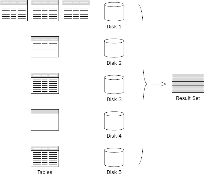
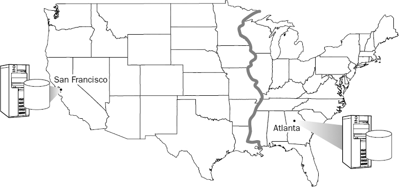
Figure 13-12
You could take a few different approaches to make data accessible from one server to another. One of the most common choices is to configure a linked server connection. A linked server maintains a connection to a database on another server as if the remote database were local. Once a linked server connection is established, tables are referenced using a four-part name, as follows:
LinkedServer.SalesDatabase.dbo.SalesDetail
What does this accomplish? Suppose I have designed the database infrastructure for a banking system. Let's say that credit card transactions may be processed in one of two data centers: one in Atlanta for east coast accounts, and one in San Francisco for west coast accounts. All U.S. customers have their account records managed in one of these two data centers. If I live in Seattle and make a purchase anywhere in the western United States, the merchant system sends my transaction to the San Francisco data center where it locates my account record and processes the transaction. However, the system must also be prepared to locate east coast account records stored in the Atlanta data center. The view used to locate all accounts (from the west coast server) may be defined like this:
CREATE VIEW vAllAccounts
AS
SELECT * FROM Accounts  -- (local West coast)
UNION ALL
SELECT * FROM EastCoastServer.SalesDatabase.dbo.Accounts -- (remote East coast)
The query issued from the client would look like this:
SELECT TOP 1 * FROM vAllAccounts WHERE CardNumber = @CardNumber
The TOP 1 statement tells the query-processing engine to stop looking after it finds one record. If the record is located in the first table (on the local server), no request is made on the remote server. Otherwise, the connection is used to pass the request to the other server, which processes the query until it locates the account record. Figure 13-13 demonstrates this scenario.
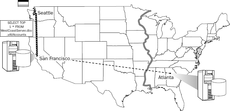
Figure 13-13
Now suppose that I travel to New York and buy a stuffed animal for my daughter's birthday. I find a great deal on a Teddy bear wearing a Yankees baseball cap and pay with my credit card, which sends a request to the Atlanta data center to Select Top 1 from a view defined as follows:
CREATE VIEW vAllAccounts
AS
SELECT * FROM Accounts  -- (local East coast)
UNION ALL
SELECT * FROM WestCoastServer.SalesDatabase.dbo.Accounts -- (remote West coast)
In this example, the east coast server doesn't find my account record in the local Accounts table so it moves to the remote server, which begins searching in its Accounts table. This part of the query is actually processed on the west coast server so data isn't unnecessarily transferred across the network connection. After finding one record (my account), it stops looking and terminates the query execution. This scenario is depicted in Figure 13-14.
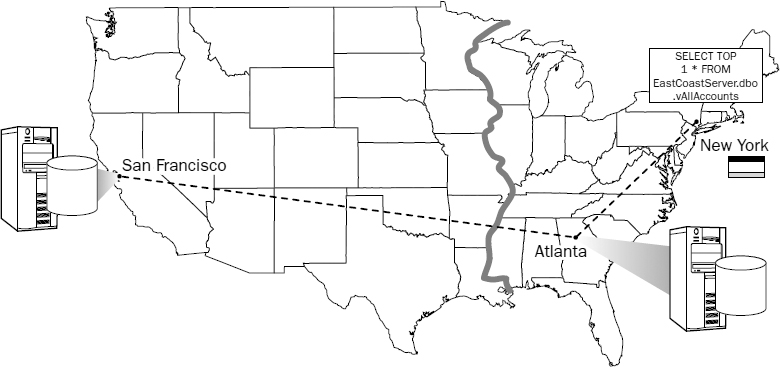
Figure 13-14
Securing Data
Another useful offering of views is to provide a layer for user data access without giving users access to sensitive data or other database objects. A common security practice is for the database administrator to lock down all of the tables, denying access to all regular users. Views are then created to explicitly expose selected tables, columns, and/or rows for all or selected users. When the select permission is granted on a view, users gain access to the view's underlying data even if the same user is explicitly denied the select permission on the underlying table(s).
Hiding Complexity
One of the most common, and arguably one of the most important reasons to use views is to simplify data access. In a normalized database, even the most basic queries can involve many different tables. Views make it possible for programmers, report writers, and users to gain access to data at a reasonably low level without having to contend with the complexities of relationships and database schema. A practical transactional database is broken down into many tables and related information is spread out across these tables to maintain data integrity and to reduce unnecessary redundancy. Reassembling all of these elements can be a headache for someone who doesn't fully understand the data or who may not be versed in relational database design. Even for the experienced developer or DBA, using a view can save time and minimize errors. The following is an example to demonstrate this point. To do something as fundamental as return employee contact information can be a relatively complex proposition.
In this example, I want to return the name, address, city, state or province, country, shift, and department information for all my employees. Because this information could be common to more than one employee, the address, state or province, country, shift, and department details are all stored in their own tables. For security reasons, I also don't want users to have access to an employee's pay rate or other private information. Using a view, users are not even aware that the columns containing this restricted information exist.
CREATE VIEW vEmployeeContactDetail
AS
SELECT Employee.EmployeeID
     , Employee.FirstName
     , Employee.LastName
     , Employee.Title
     , Employee.EmailAddress
     , Employee.BirthDate
     , Employee.Gender
     , Address.AddressLine1
     , Address.AddressLine2
     , Address.City
     , StateProvince.Name AS StateProvinceName
     , CountryRegion.Name AS CountryName
     , Address.PostalCode
     , Department.Name AS DepartmentName
     , Employee.FirstName + ‘ ’ + Employee.LastName AS ManagerName
     , Shift.Name AS ShiftName
     , Employee.HireDate
FROM   Employee
       INNER JOIN Shift
         ON Employee.ShiftID = Shift.ShiftID
       INNER JOIN Address
         ON Employee.AddressID = Address.AddressID
       INNER JOIN Department
         ON Employee.DepartmentID = Department.DepartmentID
       INNER JOIN Employee AS Manager_Employee
          ON Employee.ManagerID = Manager_Employee.EmployeeID
       INNER JOIN StateProvince
          ON Address.StateProvinceID = StateProvince.StateProvinceID
       INNER JOIN CountryRegion
          ON StateProvince.CountryRegionCode = CountryRegion.CountryRegionCode
Here's one more example of a very lengthy view. This view will be used a little later in the discussion on processing business logic in stored procedures. What I like about this view is that it contains several columns that could easily be used for reporting purposes, to sort, group, or filter the resulting data.
CREATE VIEW vProductSalesDetail
AS
SELECT TOP 100 Percent
      ProductCategory.Name AS CategoryName
    , ProductSubCategory.Name AS SubCategoryName
    , Product.Name AS ProductName
    , SalesOrderDetail.OrderQty
    , SalesOrderDetail.UnitPrice
    , SalesOrderHeader.OrderDate
    , SalesOrderHeader.TaxAmt
    , SalesOrderHeader.SubTotal
    , Customer.AccountNumber
    , Address.AddressLine1
    , Address.City
    , Address.PostalCode
    , StateProvince.StateProvinceCode
    , StateProvince.Name AS StateProvinceName
    , CountryRegion.Name AS CountryRegionName
FROM  CountryRegion
      RIGHT OUTER JOIN StateProvince
        ON CountryRegion.CountryRegionCode = StateProvince.CountryRegionCode
      RIGHT OUTER JOIN Address
        ON StateProvince.StateProvinceID = Address.StateProvinceID
      INNER JOIN CustomerAddress
        ON Address.AddressID = CustomerAddress.AddressID
      RIGHT OUTER JOIN Customer
        ON CustomerAddress.CustomerID = Customer.CustomerID
      LEFT OUTER JOIN Individual
        ON Individual.CustomerID = Customer.CustomerID
      INNER JOIN SalesOrderHeader
        ON SalesOrderHeader.CustomerID = Customer.CustomerID
      INNER JOIN SalesOrderDetail
        ON SalesOrderHeader.SalesOrderID = SalesOrderDetail.SalesOrderID
      INNER JOIN Product
         ON Product.ProductID = SalesOrderDetail.ProductID
      INNER JOIN ProductSubCategory
         ON Product.ProductSubCategoryID = ProductSubCategory.ProductSubCategoryID
      INNER JOIN ProductCategory
         ON ProductSubCategory.ProductCategoryID = ProductCategory.ProductCategoryID
Modifying Data through Views
Can data be modified through a view? Perhaps a better question is should data be modified through a view? The definitive answer is maybe. Yes, you can modify some data through views. Because a view can expose the results of a variety of query techniques, some results may be updatable, some may not, and others may allow some columns to be updated. This all depends on various join types, record-locking conditions, and permissions on the underlying tables.
As a rule, I don't think views are for updating records — that's my opinion. After all, doesn't the word view suggest that its purpose is to provide a read-only view of data? I think so, but I've also worked on enough corporate production databases where this was the only option. The fact of the matter is that over time, databases evolve. Over the years, people come and go, policies are implemented with little evidence of their purpose, and political culture dictates the methods we use. If I were king of the world, no one would have access to data directly through tables; views would provide read-only data access and support all related application features, and stored procedures would be used to perform all transactional operations and filtered data retrieval. These are the guidelines I follow when designing a system from the ground up. However, I acknowledge that this is not always possible in the typical circumstance where one database designer isn't given free license.
In simple terms, these are the most common rules governing the conditions for updating data through views:
- In an inner join, columns from one table at a time may be modified. This is due to the record-locking restrictions on related tables. Updates generally cannot be performed on two related tables within the same transaction.
- In an outer join, generally columns only for the inner table are updatable.
- Updates can't be performed through a view containing a UNION query.
Stored Procedures
If views raise the bar of database functionality, then stored procedures take it to the next level. Unlike views, stored procedures can be used for much more than reading data. They provide a wide range of programming functionality. Categorically, stored procedures can be used to do the following:
- Implement parameterized views
- Return scalar values
- Maintain records
- Process business logic
In the following examples, I've prefixed the names with the letters sp for stored procedure. If you use the Object Browser to view system stored procedure names, you'll see that most of these existing procedures are prefixed with sp_. It's not a good idea to use the same prefix as the system procedures because this is an indicator to the database engine to try to locate this procedure in the system catalog before it looks in your database. Although there are no specific compatibility issues with this prefix, this can degrade performance and cause potential confusion.
Stored Procedures as Parameterized Views
Like views, stored procedures can be used to return a result set based on a SELECT statement. However, I want to clarify an important point about the difference between views and stored procedures. A view is used in a SELECT statement as if it were a table. A stored procedure is executed, rather than selected from. For most programming APIs, this makes little difference. If a programmer needs to return a set of rows to an application or report, ActiveX Data Objects (ADO) or ADO.NET can be used to obtain results from a table, a view, or a stored procedure.
A stored procedure can be used in place of a view to return a set of rows from one or more tables. Earlier in this chapter, I used a simple view to return selected columns from the Product table. Again, the script looks like this:
CREATE VIEW vProductCosts
AS
SELECT ProductID, ProductSubcategoryID, Name, ProductNumber, StandardCost
FROM Product
Contrast this with the script to create a similar stored procedure:
CREATE PROCEDURE spProductCosts
AS
SELECT ProductID, ProductSubcategoryID, Name, ProductNumber, StandardCost
FROM Product
To execute the new stored procedure, the name is preceded by the EXECUTE statement:
EXECUTE spProductCosts
Although this is considered the most proper syntax, the following are also examples of acceptable syntax.
The shorthand version of EXECUTE:
EXEC spProductCosts
No EXECUTE statement:
spProductCosts
Using Parameters
A parameter is a special type of variable used to pass values into an expression. Named parameters are used for passing values into and out of stored procedures and user-defined-functions. Parameters are most typically used to input, or pass values into, a procedure, but can also be used to return values.
Parameters are declared immediately after the procedure definition and before the term AS. Parameters are declared with a specific data type and are used as variables in the body of a SQL statement. I will modify this procedure with an input parameter to pass the value of the ProductSubCategoryID. This will be used to filter the results of the query. This example shows the script for creating the procedure. If the procedure already exists, the CREATE statement may be replaced with the ALTER statement:
ALTER PROCEDURE spProductCosts
@SubCategoryID Int
AS
SELECT ProductID, Name, ProductNumber, StandardCost
FROM Product
WHERE ProductSubCategoryID = @SubCategoryID
To execute the procedure and pass the parameter value in SQL Query Analyzer or the Query Editor, simply append the parameter value to the end of the statement, like this:
EXECUTE spProductCosts 1
Alternatively the stored procedure can be executed with the parameter and assigned value like this:
EXECUTE spProductCosts @SubCategory = 1
Stored procedures can accept multiple parameters and the parameters can be passed in either by position or by value similar to the previous example. Suppose I want a stored procedure that filters products by subcategory and price. It would look something like this:
CREATE PROCEDURE spProductsByCost
@SubCategoryID Int, @Cost Money
AS
SELECT ProductID, Name, ProductNumber, StandardCost
FROM Product
WHERE ProductSubCategoryID = @SubCategoryID
AND StandardCost > @Cost
Using SQL, the multiple parameters can be passed in a comma-delimited list in the order they were declared:
EXECUTE spProductsByCost 1, $1000.00
Or the parameters can be passed explicitly by value. If the parameters are supplied by value it doesn't matter in what order they are supplied:
EXECUTE spProductsByCost @Cost = $1000.00, @SubCategoryID = 1
If a programmer is using a common data access API such as ADO or ADO.NET, separate parameter objects are often used to encapsulate these values and execute the procedure in the most efficient manner.
Although views and stored procedures do provide some overlap in functionality, they each have a unique purpose. The view used in the previous example can be used in a variety of settings where it may not be feasible to use a stored procedure. However, if I need to filter records using parameterized values, a stored procedure will allow me to do this where a view will not. So, if the programmer building the product browse screen needs an unfiltered result set and the report designer needs a filtered list of products based on a subcategory parameter, do I create a view or a stored procedure? That's easy, both. Use views as the foundation upon which to build stored procedures. Using the previous example, I select from the view rather than the table:
ALTER PROCEDURE spProductCosts
@SubCategoryID Int
As
SELECT ProductID, Name, ProductNumber, StandardCost
FROM vProductCosts
WHERE ProductSubCategoryID = @SubCategoryID
The benefit may not be so obvious in this simple, one-table example. However, if a procedure were based on the seven-table vEmployeeContactDetail view, the procedure call might benefit from optimizations in the view design and the lower maintenance cost of storing this complex statement in only one object.
Returning Values
The parameter examples shown thus far demonstrate how to use parameters for passing values into a stored procedure. One method to return a value from a procedure is to return a single-column, single-row result set. Although there is probably nothing grossly wrong with this technique, it's not the most effective way to handle simple values. A result set is wrapped in a cursor, which defines the rows and columns, and may be prepared to deal with record navigation and locking. This kind of overkill reminds me of a digital camera memory card I recently ordered from a discount electronics supplier. A few days later, a relatively large box arrived and at first appeared to be filled with nothing more than foam packing peanuts. I had to look carefully to find the postage-size memory card inside.
In addition to passing values into a procedure, parameters can also be used to return values for output. Stored procedure parameters with an OUTPUT direction modifier are set to store both input and output values by default. Additionally, the procedure itself is equipped to return a single integer value without needing to define a specific parameter. The return value is also called the return code and defaults to the integer value of 0. Some programming APIs such as ADO and ADO.NET actually create a special output parameter object to handle this return value. Suppose I want to know how many product records there are for a specified subcategory. I'll pass the SubCategoryID using an input parameter and return the record count using an output parameter:
CREATE PROCEDURE spProductCountBySubCategory
  @SubCategoryID Int,
  @ProdCount Int OUTPUT
AS
  SELECT @ProdCount = COUNT(*)
  FROM Product
  WHERE ProductSubCategoryID = @SubCategoryID
To test a stored procedure with output parameters in the Management Studio or Query Analyzer environments, it is necessary to explicitly use these parameters by name. Treat them as if they were variables but you don't need to declare them. When executing a stored procedure using SQL, the behavior of output parameters can be a bit puzzling because they also have to be passed in. In this example, using the same stored procedure, a variable is used to capture the output parameter value. The curious thing about this syntax is that the assignment seems backwards. Remember that the OUTPUT modifier affects the direction of the value assignment—in this case, from right to left:
DECLARE @Out Int

EXECUTE spProductCountBySubCategory
@SubCategoryID = 2,
@ProdCount = @Out OUTPUT

SELECT @Out AS ProductCountBySubCategory
ProductCountBySubCategory
------------------------
184
It is critical that the OUTPUT modifier also be added to the output parameter when it is passed in to the stored procedure. If you don't, the stored procedure will still execute, but it will not return any data.
DECLARE @Out Int

EXECUTE spProductCountBySubCategory
@SubCategoryID = 2,
@ProdCount = @Out --Missing the OUTPUT directional modifier

SELECT @Out AS ProductCountBySubCategory
ProductCountBySubCategory
-------------------------
NULL
There is no practical limit to the number of values that may be returned from a stored procedure. The stated limit is 2,100, including input and output parameters.
If you need to return only one value from the procedure, this can be done without the use of an output parameter using the return code of the procedure as long as the value being returned is an integer. Here is the same stored procedure showing this technique:
CREATE PROCEDURE spProductCountBySubCategory
   @SubCategoryID Int
AS
   DECLARE @Out Int
   SELECT @Out = Count(*)
   FROM Product
   WHERE ProductSubCategoryID = @SubCategoryID
RETURN @Out
The RETURN statement does two things: it modifies the return value for the procedure from the default value, 0, and it terminates execution so that any statements following this line do not execute. This is significant in cases where there may be conditional branching logic. Typically the capture of the return value must be done with a programming API. Executing this stored procedure in Query Analyzer or Management Studio will not return any results because these interfaces don't display the procedure's return value by default.
Record Maintenance
Using stored procedures to manage the insert, update, and delete operations for each major database entity can drastically reduce the cost of data maintenance tasks down the road. Any program code written to perform record operations should do so using stored procedures and not ad-hoc SQL expressions. As a rule of thumb, when I design a business application, every table that will have records managed through the application interface gets a corresponding stored procedure to perform each of these operations. These procedures are by far the most straightforward in terms of syntax patterns. Although simple, writing this script can be cumbersome due to the level of detail necessary to deal with all of the columns. Fortunately, the SQL Server 2000 Query Analyzer and the SQL Server 2005 Management Studio include scripting tools that will generate the bulk of the script for you. Beyond creating the fundamental Insert, Update, Delete, and Select statements, you need to define and place parameters into your script.
Insert Procedure
The basic pattern for creating an Insert stored procedure is to define parameters for all non-default or auto-populated columns. In the case of the Product table, the ProductID primary key column will automatically be incremented because it's defined as an identity column; the rowguid and ModifiedDate columns have default values assigned in the table definition. The MakeFlag and FinishedGoodsFlag columns also have default values assigned in the table definition, but it may be appropriate to set these values differently for some records. For this reason, these parameters are set to the same default values in the procedure. Several columns are nullable and the corresponding parameters are set to a default value of null. If a parameter with a default assignment isn't provided when the procedure is executed, the default value is used. Otherwise, all parameters without default values must be supplied:
CREATE PROCEDURE spProduct_Insert
        @Name                   nVarChar(50)
     ,  @ProductNumber          nVarChar(25)
     ,  @MakeFlag               Bit         = 1
     ,  @FinishedGoodsFlag      Bit         = 1
     ,  @Color                  nVarChar(15)  = Null
     ,  @SafetyStockLevel       SmallInt
     ,  @ReorderPoint           SmallInt
     ,  @StandardCost           Money
     ,  @@ListPrice             Money
     ,  @Size                   nVarChar(5)   = Null
     ,  @SizeUnitMeasureCode        nChar(3)      = Null
     ,  @WeightUnitMeasureCode  nChar(3)      = Null
     ,  @Weight             Decimal       = Null
     ,  @DaysToManufacture      Int
     ,  @ProductLine            nChar(2)      = Null
     ,  @Class                  nChar(2)      = Null
     ,  @Style                  nChar(2)      = Null
     ,  @ProductSubcategoryID       SmallInt      = Null
     ,  @ProductModelID         Int           = Null
     ,  @SellStartDate          DateTime
     ,  @SellEndDate            DateTime      = Null
     ,  @DiscontinuedDate       DateTime      = Null
AS
INSERT INTO Product
   (   Name
     , ProductNumber
     , MakeFlag
     , FinishedGoodsFlag
     , Color
     , SafetyStockLevel
     , ReorderPoint
     , StandardCost
     , ListPrice
     , Size
     , SizeUnitMeasureCode
     , WeightUnitMeasureCode
     , Weight
     , DaysToManufacture
     , ProductLine
     , Class
     , Style
     , ProductSubcategoryID
     , ProductModelID
     , SellStartDate
     , SellEndDate
     , DiscontinuedDate )
SELECT
       @Name
     , @ProductNumber
     , @MakeFlag
     , @FinishedGoodsFlag
     , @Color
     , @SafetyStockLevel
     , @ReorderPoint
     , @StandardCost
     , @ListPrice
     , @Size
     , @SizeUnitMeasureCode
     , @WeightUnitMeasureCode
     , @Weight
     , @DaysToManufacture
     , @ProductLine
     , @Class
     , @Style
     , @ProductSubcategoryID
     , @ProductModelID
     , @SellStartDate
     , @SellEndDate
     , @DiscontinuedDate
It's a lot of script but it's not complicated. Executing this procedure in SQL is quite easy. This can be done in comma-delimited fashion or by using explicit parameter names. Because the majority of the fields and corresponding parameters are optional, they can be ommitted. Only the required parameters need to be passed; the optional parameters are simply ignored:
EXECUTE spProduct_Insert
    @Name               = ‘Widget’
  , @ProductNumber      = ‘987654321’
  , @SafetyStockLevel   = 10
  , @ReorderPoint       = 15
  , @StandardCost       = 23.50
  , @ListPrice          = 49.95
  , @DaysToManufacture  = 30
  , @SellStartDate      = ‘10/1/04’
The procedure can also be executed with parameter values passed in a comma-delimited list. Although he script isn't nearly as easy to read, it is less verbose. Even though this may save you some typing, it often becomes an exercise in counting commas and rechecking the table's field list in the Object Browser until the script runs without error.
EXECUTE spProduct_Insert ‘Widget’, ‘987654321’, 1, 1, Null, 10, 15, 23.50, 49.95,
Null, Null, Null, Null, 30, Null, Null, Null, Null, Null, ‘10/1/04’
When using this technique, parameter values must be passed in the order they are declared. Values must be provided for every parameter up to the point of the last required value. After that, the remaining parameters in the list can be ignored.
A useful variation of this procedure may be to return the newly generated primary key value. The last identity value generated in a session is held by the global variable, @@Identity. To add this feature, simply add this line to the end of the procedure. This would cause the Insert procedure to return the ProductID value for the inserted record.
RETURN @@Identity
Of course, if you have already created this procedure, change the CREATE keyword to ALTER, make changes to the script, and then re-execute it.
Update Procedure
The Update procedure is similar. Usually when I create these data maintenance stored procedures, I write the script for the Insert procedure and then make the modifications necessary to transform the same script into an Update procedure. As you can see, it's very similar:
CREATE PROCEDURE spProduct_Update
        @ProductID              Int
      , @Name               nVarChar(50)
      , @ProductNumber          nVarChar(25)
      , @MakeFlag               Bit           = 1
      , @FinishedGoodsFlag      Bit           = 1
      , @Color              nVarChar(15)  = Null
      , @SafetyStockLevel       SmallInt
      , @ReorderPoint             SmallInt
      , @StandardCost             Money
      , @ListPrice          Money
      , @Size               nVarChar(5)   = Null
      , @SizeUnitMeasureCode    nChar(3)      = Null
      , @WeightUnitMeasureCode   nChar(3)       = Null
      , @Weight                Decimal      = Null
      , @DaysToManufacture      Int
      , @ProductLine              nChar(2)      = Null
      , @Class                 nChar(2)     = Null
      , @Style                 nChar(2)     = Null
      , @ProductSubcategoryID   SmallInt        = Null
      , @ProductModelID      Int            = Null
      , @SellStartDate            DateTime
      , @SellEndDate              DateTime      = Null
      , @DiscontinuedDate        DateTime      = Null
AS
UPDATE  Product
SET      Name                   = @Name
     ,  ProductNumber           = @ProductNumber
     ,  MakeFlag                = @MakeFlag
     ,  FinishedGoodsFlag       = @FinishedGoodsFlag
     ,  Color               = @Color
     ,  SafetyStockLevel        = @SafetyStockLevel
     ,  ReorderPoint            = @ReorderPoint
     , StandardCost            = @StandardCost
     ,  ListPrice               = @ListPrice
     ,  Size                    = @Size
     ,  SizeUnitMeasureCode     = @SizeUnitMeasureCode
     ,  WeightUnitMeasureCode   = @WeightUnitMeasureCode
     ,  Weight              = @Weight
     ,  DaysToManufacture       = @DaysToManufacture
     ,  ProductLine         = @ProductLine
     ,  Class               = @Class
     ,  Style               = @Style
     ,  ProductSubcategoryID    = @ProductSubcategoryID
     ,  ProductModelID          = @ProductModelID
     ,  SellStartDate           = @SellStartDate
     ,  SellEndDate         = @SellEndDate
     ,  DiscontinuedDate        = @DiscontinuedDate
WHERE ProductID             = @ProductID
The parameter list is the same as the Insert procedure with the addition of the primary key, in this case, the ProductID column.
Delete Procedure
In its basic form, the Delete procedure is very simple. The only necessary parameter is for the ProductID column value:
CREATE PROCEDURE spProduct_Delete
     @ProductID    Int
AS
     DELETE FROM Product
     WHERE ProductID = @ProductID
Handling and Raising Errors
A common choice you may need to make in many data maintenance procedures is how you will handle errors. Attempting to insert, update, or delete a record that violates constraints or rules will cause the database engine to raise an error. If this is acceptable behavior, you don't need to do anything special in your procedure code. When the procedure is executed, an error is raised and the transaction is aborted. You simply need to handle the error condition in the client program code. Another, often more desirable, approach would be to proactively investigate the potential condition and then raise a custom error. This may have the advantage of offering the user or client application more useful error information or a more graceful method to handle the condition. In the case of the Delete procedure, I could check for existing dependent records and then raise a custom error without attempting to perform the delete operation. This also has the advantage of not locking records while the delete operation is attempted.
Error Handling in SQL Server 2000
For many years, the ability to handle errors in Transact-SQL script has been limited to the same type of pattern used in other scripting languages. The query-processing engine is not equipped to respond to error conditions in the same way that an event-driven run-time engine would. What this boils down to is that if you suspect that an error might be raised after a specific line of script, you can check for an error condition and respond to it. The downside to this approach is that you have to be able to guess where an error might occur and be prepared to respond to it.
There are two general approaches to raising errors. One is to raise the error on-the-fly. This is done using a single statement. The other approach is to add custom error codes and message text to the system catalog. These messages can then be raised from script in any database on the server. Custom errors are added to the system catalog using the sp_AddMessage system stored procedure. Here's an example:
sp_AddMessage @msgnum=50010
            , @severity=16
            , @msgtext=‘Cannot delete a product with existing sales order(s).’
            , @with_log=‘True’
            , @replace=‘Replace’
Three parameters are required: the message number, message severity, and message text. There are also three additional optional parameters: one to specify logging the error in the server's application log, one for replacing a current error with the same message number, and one to specify the language of the error if multiple languages are installed on the server. Custom error numbers begin at 50,001. This is user-assigned and has no special meaning. It's just a unique value. The system recognizes severity values within specified numeric ranges and may respond by automatically logging the error or sending alerts. Alerts are configurable within the SQL Server Agent. Messages and errors are distinguished by the Severity Level flag. Those with a severity level from 0 to 10 are considered to be informational messages and will not raise a system exception. Those with a severity level from 11 to 18 are non-fatal errors, and those 19 or above are considered to be most severe. This scale was devised for Windows service error logging. The following table shows the system-defined error severity levels.
| Severity Level | Description |
| 1 | Misc. System Information |
| 2-6 | Reserved |
| 7 | Notification: Status Information |
| 8 | Notification: User Intervention Required |
| 9 | User Defined |
| 10 | Information |
| 11 | Specified Database Object Not Found |
| 12 | Unused |
| 13 | User Transaction Syntax Error |
| 14 | Insufficient Permission |
| 15 | Syntax Error in SQL Statements |
| 16 | Misc. User Error |
| 17 | Insufficient Resources |
| 18 | Fatal Error in Resource |
| 19* | Fatal Error in Resource |
| 20* | Fatal Error in Current Process |
| 21* | Fatal Error in Database Processes |
| 22* | Fatal Error: Table Integrity Suspect |
| 23* | Fatal Error: Database Integrity Suspect |
| 24* | Fatal Error: Hardware Error |
| 25* | Fatal Error |
* Messages with a severity level 19 or above will automatically be logged in the server's application log. When an error is raised in the procedure, you also have the option to explicitly log the message regardless of the severity level.
When logging an error in the application log, errors with a severity level less than 14 will be recorded as informational. Level 15 is recorded as a warning, and levels greater than 15 are issued the error status.
This example demonstrates raising a previously declared error:
RAISERROR (50010, 16, 1)
The output from this expression returns the message defined earlier:
Msg 50010, Level 16, State 1, Line 1
Cannot delete a product with existing sales orders.
The severity level is actually repeated in the call. I know, this seems like a strange requirement, but that's the way it works. It also does not have to be the same as the defined severity level. If I want to raise the error as a severity level 11 instead of the 16 I created it with, I can. The last parameter is the state. This value is user-defined and has no inherent meaning to the system, but it is a required argument. State can be a signed integer between -255 and +255. State can be used for internal tracking, for example, to track all “State 3” errors.
Here is an example of an ad-hoc message that has not been previously defined:
RAISERROR (‘The sky is falling’, 16, 1)
The resulting output is as follows:
Msg 50000, Level 16, State 1, Line 1
The sky is falling
Note that ad-hoc messages use the reserved message id of 50000. Raising an ad-hoc message with a severity level of 19 or higher requires elevated privileges and must be performed with explicit logging. If you need to raise an error of this type, it's advisable to define these messages ahead of time.
When an error occurs, the global variable, @@ERROR, changes from its default value of 0 to an integer type standard error number. SQL Server 2000 can return more than 3800 standard errors and SQL Server 2005 includes more than 6800 unique errors. All of these error numbers and messages are stored in the Master database.
This example is a simple stored procedure using a generic approach to error handling:
CREATE PROCEDURE spRunSQL
 @Statement VarChar(2000)
AS
DECLARE @StartTime DateTime
      , @EndTime DateTime
      , @ExecutionTime Int
 SET @StartTime = GetDate()
 EXECUTE (@Statement)
 IF @@Error = 0
      BEGIN
       SET @EndTime = GetDate()
       SET @ExecutionTime = DateDiff(MilliSecond, @StartTime, @EndTime)
       RETURN @ExecutionTime
    END
Without the error-checking script, the remaining statements would be executed after the erroneous EXCUTE… line. The following example uses a more specific approach. This assumes that I want to replace the default error message and numbers with my own:
CREATE PROCEDURE spRunSQL
  @Statement VarChar(2000) -- Input param. accepts any SQL statement.
AS
  DECLARE @StartTime DateTime
        , @EndTime DateTime
       , @ExecutionTime Int
       , @ErrNum Int
  SET @StartTime = GetDate()
  EXECUTE (@Statement)
  SET @ErrNum = @@Error
    IF @ErrNum = 207         -- Bad column
      RAISERROR (‘Bad column name’, 16, 1)
    ELSE IF @ErrNum = 208    -- Bad object
      RAISERROR (‘Bad object name’, 16, 1)
    ELSE IF @ErrNum = 0       -- No error. Resume.
     BEGIN
      SET @EndTime = GetDate()
      SET @ExecutionTime = DateDiff(MilliSecond, @StartTime, @EndTime)
       RETURN @ExecutionTime -- Return execution time in milliseconds
     END
Just a note about this example: I chose to use this scenario because it was easy to demonstrate. Under the right conditions, and with appropriate security constraints, this can be a very useful procedure. However, you should be very cautious about enabling a stored procedure that allows users to execute any SQL statements they choose. Otherwise, users who are otherwise restricted from executing certain statements could work around these restrictions.
Error Handling in SQL Server 2005
One of the most significant enhancements to Transact-SQL is its new error-handling capability. In the previous discussion, you saw how it was necessary to check for errors after each statement. In SQL Server 2005, error handling is much like some modern programming languages (such as C#, Java, and VB.NET). The new pattern is quite easy to implement and will be familiar to you if you have worked with newer programming languages. Any statements that could possibly cause an error to be raised are wrapped within a TRY block. The error-handling script is located in a separate CATCH block. When an error condition occurs in the TRY block, execution is moved to the first line within the CATCH block. The limitation of SQL Server 2005 error handling is that it can only be used to retrieve error information and to significantly reduce the amount of error code required, but it cannot in a true sense of the word “handle” errors. Once an error occurs inside a transaction the transaction enters a Doomed state. The error can only be recorded and maybe some other event code executed, but the transaction will have to be reissued.
BEGIN TRY
   … Transaction
END TRY
BEGIN CATCH
   … error-handing script
  END CATCH
This is an example using this form of error handling:
CREATE PROCEDURE spDeleteProduct @Productid int
AS
BEGIN TRY
 BEGIN TRANSACTION
 DELETE Product WHERE ProductID = @ProductID
 COMMIT TRANSACTION
END TRY
BEGIN CATCH
 DECLARE @Err AS int
 DECLARE @Msg AS varchar(max)
 SET @Err = @@Error
 SET @Msg = Error_Message()
 ROLLBACK TRANSACTION
 INSERT ErrorTable
 VALUES (@err, @msg)
END CATCH
Processing Business Logic
Handling business rules is all about making decisions. The decision structures in Transact-SQL are uncomplicated. When I need to write a decision statement, the first thing I typically do is state the logic using natural language. Transact-SQL's roots are in the English language. You'll recall from Chapter 1 that IBM's predecessor to SQL was actually called SEQUEL, which stood for Structured English Query Language. You should be able to break down any process into a decision tree. Even complex logic, once distilled into fundamental components, is just a series of simple logical combinations. This concept is what I call compounded simplicity—each individual piece is simple, there just may be a lot of pieces.
Using logical operators within SQL statements, you should be able to handle quite a lot of relatively complex business logic. I find that my first attempt to address a complex problem is usually a bit convoluted. After taking some time to approach the problem from different angles, I'm usually more successful in using a simpler technique. It takes a little patience and a few iterations to get to the optimal solution.
In the previous section on views, I created a complex view called vProductSalesDetail. This view is an excellent example of the kind of data my sales manager may want to see in a report. Suppose I plan to use SQL Server Reporting Services to design a sales detail report. Users have asked for the ability to provide a variety of parameter values to be used for filtering. As a rule, if a parameter is provided, the report data is filtered accordingly. If the parameter value is not provided, the parameter is ignored and no related filtering takes place. The report parameters are listed in the following table.
| Parameters | Logic |
| Sales Order From Date and Sales Order To Date | The user is prompted to type a date value for each of these parameters. If both parameters contain a value, the sales order data is filtered within the given range of order dates. If either of the parameters is not provided, this criterion is ignored. |
| Account Number | The user is prompted to type a customer's account number. If this value is not provided, this criterion is ignored. |
| Product Category | The product category is selected from a drop-down list. The first item of the list displays the word “All.” If this value is selected, records are not filtered by the product category. |
Combining logical operators may seem to be very complicated but it's actually quite simple when broken down into core components. Each branch of logic must be isolated from others that it shouldn't affect. Using parentheses, group these statements together. For example, if the account number parameter is not provided (the value is Null), you need not consider the value of the corresponding column. In SQL, this logic would look like this:
The inner parentheses, surrounding each individual statement, just make this statement easier to read and could be omitted. The outer parentheses isolate this logic from any other statements. If the value of the parameter @ProductCategory is NULL, then it doesn't matter whether the CategoryName column value matched the parameter value or not. One side of the OR expression has already been satisfied so the expression on other side need not be true as well.
Because I want to filter the entire result set based on combinations of multiple parameters, each group of parameters-related statements are combined using the AND operator. This is because one of the two statements on the OR statement must be true to return any records for that part of the WHERE clause. Combining the logic for two parameters looks like this:
((@ProductCategory IS NULL) OR (CategoryName = @ProductCategory))
AND
((@ProductCategory = ‘All’) OR (CategoryName = @ProductCategory))
I changed the logic for the product category to check for the word “All” just to mix this up a little. It would be convenient if all parameters were compared in the same way, but this is a very realistic scenario. Putting it all together, the stored procedure might look like the following. Notice how the actual selection and column referencing is very simple. This is because I've already handled the complexity of the query in the view. The procedure simply leverages this investment.
CREATE PROCEDURE spProductSalesDetail
   @SalesOrderDateFrom DateTime = Null,
   @SalesOrderDateTo   DateTime = Null,
   @ProductCategory    nVarChar(50) = ‘All’,
   @AccountNumber      VarChar(10) = Null
AS
SELECT * FROM vProductSalesDetail
WHERE
  ((@SalesOrderDateFrom Is Null) OR (@SalesOrderDateTo Is Null))
  OR
  (OrderDate BETWEEN @SalesOrderDateFrom AND @SalesOrderDateTo)
  AND
  ((@ProductCategory = ‘All’) OR (CategoryName = @ProductCategory))
  AND
  ((@AccountNumber Is Null) OR (AccountNumber = @AccountNumber))
Try It Out
Test this procedure by supplying some parameters and not others. You should be able to use any combination of parameters. You can even leave off the product category because this parameter defaults to the value All. For example:
EXECUTE spProductSalesDetail
@SalesOrderDateFrom = ‘12-1-03’,
@SalesOrderDateTo   = ‘12-31-03’,
@ProductCategory    = ‘Bike’
Conditional Logic
At the very core of all logic is the simple word “If” in the English language. All other decision structures are variations or extensions of the same basic if concept. Before I show you the specific SQL syntax, take a look at some simple phrases that are examples of conditional logic:
If a product record exists, update it.
If a product record doesn't exist, create one.
If a backorder record exists and sufficient inventory exists, delete the backorder and ship the product.
What happens if this condition is not met? That's easy. This is done using an Else statement:
If an account balance is current, calculate the new total.
…or else if the account balance is past due, add a late fee and calculate the new total.
…or else if the account is seriously past due, add a late fee, close the account, and calculate the new total.
Most programming languages include some other forms of logical branching statements that extend the If statement paradigm. For example, the Visual Basic Select Case command just consolidates what would otherwise be several if… else statements. Transact-SQL contains a Select Case structure that is quite different, which will be introduced shortly.
IF
In SQL, the IF statement is not followed by the word Then. If a condition is met (if the outcome is True), script beginning on the next line is simply executed. This stored procedure checks for the named table in the database catalog:
CREATE PROCEDURE spTableExists
  @TableName VarChar(128)
AS
  IF EXISTS(SELECT * FROM sysobjects WHERE name = @TableName)
    PRINT @TableName + ‘ exists’
The ELSE statement, in this case, simply allows me to execute another line of script when the condition is not met:
CREATE PROCEDURE spTableExists
   @TableName VarChar(128)
AS
  IF EXISTS(SELECT * FROM sysobjects WHERE name = @TableName)
    PRINT @TableName + ‘ exists’
  ELSE
    PRINT @TableName + ‘ doesn't exist’
When multiple lines of code follow an IF statement it is best to wrap the lines in a BEGIN… END block. Although this is not strictly required, it makes the code much simpler to read and debug.
Try It Out
Using the AdventureWorks database, create a stored procedure to return product information. An optional parameter will be used to determine when records will be filtered. The query uses the Product and ProductSubCategory tables so you can pass the subcategory name for filtering. This is a lot of script to type so you might consider using the Query Builder to create the basic SELECT statement. The input parameter, @Category, is set to Null so it becomes optional.
CREATE PROCEDURE spGetProductByCategory
 @Category nVarChar(50) = NULL
AS
IF @Category IS NULL
 BEGIN
   SELECT PC.Name AS ProductCategory
        , P.ProductID
        , P.Name AS ProductName
   FROM Product AS P
   INNER JOIN ProductSubCategory AS PSC
   ON P.ProductSubCategoryID = PSC.ProductSubCategoryID
   INNER JOIN ProductCategory AS PC
   ON PSC.ProductCategoryID = PC.ProductCategoryID
END
ELSE
 BEGIN
    SELECT PC.Name AS ProductCategory
         , P.ProductID
         , P.Name AS ProductName
    FROM Product AS P
    INNER JOIN ProductSubCategory AS PSC
    ON P.ProductSubCategoryID = PSC.ProductSubCategoryID
    INNER JOIN ProductCategory AS PC
    ON PSC.ProductCategoryID = PC.ProductCategoryID
    WHERE PC.Name = @Category
END
If the procedure is executed without a category name value, all product records are returned. Otherwise, the results are filtered. Now, try this out. Execute the procedure with and without a category parameter value:
EXECUTE spProductGetByCategory ‘Bikes’
By passing the category ‘Bikes’, only 97 product records are returned because the results are filtered by this category, as shown in Figure 13-15.
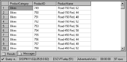
Figure 13-15
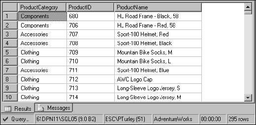
Now execute the procedure without a category value:
EXECUTE spProductGetByCategory
This time, 295 rows (give or take a few depending on other sample queries you may have run) are returned because the products are unfiltered, as shown in Figure 13-16.
CASE
The purpose of the CASE statement is to return a specified value based on a set of business logic. A variety of useful applications for the CASE statement include translating abbreviations into descriptive values and simulating look-up table joins.
The syntax pattern looks like this:
SELECT CASE value to evaluate
WHEN literal value 1 THEN return value
WHEN literal value 2 THEN return value
…
END
Here's a simple example that could be applied to a status indicator value:
DECLARE @Status Int
SET @Status = 1

SELECT CASE @Status
  WHEN 1 THEN ‘Active’
  WHEN 2 THEN ‘Inactive’
  WHEN 3 THEN ‘Pending’
END
Now, I'll plug the same logic into a query, replacing what would otherwise be an outer join to a related table, with a CASE expression:
SELECT ProductID
  , Name
  , ListPrice
  , CASE ProductSubCategoryID
      WHEN 1 THEN ‘Mountain Bike’
      WHEN 2 THEN ‘Road Bike’
      WHEN 3 THEN ‘Touring Bike’
      WHEN Null THEN ‘Something Else’
      ELSE ‘(No Subcategory)’
    END As SubCategory
FROM Product
This script effectively creates an alias column called SubCategory. You can use it with a different aliasing technique, in this case, using the column = … syntax:
SELECT ProductID
   , Name
   , ListPrice
   , SubCategory = CASE ProductSubCategoryID
       WHEN 1 THEN ‘Mountain Bike’
       WHEN 2 THEN ‘Road Bike’
       WHEN 3 THEN ‘Touring Bike’
       WHEN Null THEN ‘Something Else’
       ELSE ‘(No Subcategory)’
    END
FROM Product
Either way, the results are the same. Note that I've filtered these results to show a variety of values by adding WHERE ListPrice > 2000. You don't need to do the same because you can scroll through the results as shown in Figure 13-17.
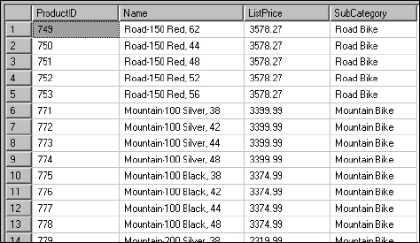
Figure 13-17
Looping
Statements can be repeated in a conditional looping structure. Looping is performed with the WHILE statement and an expression returning a Boolean result. In the following example, a separate WHERE statement is executed for each iteration of the loop, filtering on the corresponding product subcategory ID.
Try It Out
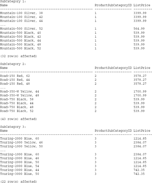
Switch the query results from grid to text and execute the following:
DECLARE @Counter Int
SET @Counter = 1
WHILE @Counter < 4
  BEGIN
      PRINT ‘’
      PRINT ‘SubCategory ’
           + CONVERT(VarChar(10), @Counter) + ‘:’
   SELECT Name, ProductSubCategoryID, ListPrice
      FROM Product
      WHERE ProductSubCategoryID = @Counter

    SET @Counter = @Counter + 1
  END
The results show three separate lists for each of the subcategories:
During the loop, you may need to modify the logic of some operations. The BREAK statement exits the WHILE structure, resuming execution after the END statement. The CONTINUE statement doesn't exit the loop but sends execution back up to the WHILE statement to repeat the loop:
/* If the avg price for all products is below $1200,
   raise all prices by 25% until avg is $1200 or higher
   or highest price is over $4000.
*/
WHILE (SELECT AVG(ListPrice) FROM Product) < $1200
BEGIN
   UPDATE Product SET ListPrice = ListPrice * 1.25
   SELECT MAX(ListPrice) FROM Product
   IF (SELECT MAX(ListPrice) FROM Product) > $4000
      -- Greatest price is too high, quit.
      BREAK
   ELSE
      -- Prices are within range, continue to loop.
      CONTINUE
END
PRINT ‘Done.’
User-Defined Functions
When user-defined functions were introduced in SQL Server 2000, this opened the door to a whole new level of functionality. Until then, nearly all business logic had to be in compound expressions with little opportunity to reuse code. In traditional programming languages, functions typically accept any number of values and then return a scalar (single) value. Functions are typically used to perform calculations, to compare, parse, and manipulate values. This describes one of the capabilities of user-defined functions (UDFs), but they can also be used to return sets of data.
Set-based functions can be parameterized like a stored procedure but are used in a SELECT expression like a view. In some ways this makes UDFs the best of both worlds. Three different categories of user-defined functions exist, two of which return result sets. These categories include the following:
- Scalar functions
- Multi-statement table-valued functions
- Inline table-valued functions
One important thing to keep in mind when designing user-defined functions is that other functions called within the script must be deterministic. In other words, the value returned must be dependent only on the value(s) passed to it, and not based on external resources. For example, a UDF cannot call a nondeterministic GetDate() function. Instead, to deal with this limitation, you would pass the date value into the function as a parameter.
Scalar Functions
A scalar function accepts any number of parameters and returns one value. The term scalar differentiates a single, “flat” value from more complex structured values, such as arrays or result sets. This pattern is much like that of traditional functions written in common programming languages.
The script syntax is quite simple. Input parameters are declared within parentheses followed by the return value declaration. All statements must be enclosed in a BEGIN… END block. In this simple example, I calculate the age by getting the number of days between the birth date and today's date. Because my function can't call the nondeterministic GETDATE() function, this value must be passed into the function using the @Today parameter. The number of days is divided by the average number of days in a year to determine the result:
CREATE FUNCTION fnGetAge (@BirthDate DateTime, @Today DateTime)
 RETURNS Int
AS
 BEGIN
     RETURN DateDiff(day, @BirthDate, @Today) / 365.25
 END
When a scalar function is called without specifying the owner or schema, SQL Server assumes it to be a built-in function in the system catalog. For this reason, user-defined scalar functions are always called using multi-part names, prefixed at least with the owner or schema name:
SELECT dbo.fnGetAge(‘1/4/1962’, GetDate())
Before writing the next sample function, I'd like to create a set of data to use. Assume that you are in charge of preparing invitations to your annual company picnic. The HR department manager has exported a list of employees from the personnel system to a text file. You have used DTS to import this data into SQL Server and now you need to format the data for the invitations. Names are in a single column in the form: LastName, FirstName. You need to separate the first name and last name values into two columns.
The business logic for parsing the last name and first name values is very similar. The logic for extracting the last name is as follows:
- Find the position of the delimiting comma.
- Identify the last name value from the first character through the character one position before the comma.
- Return this value from the function.
Translating this logic into SQL, the function definition looks like this:
CREATE FUNCTION fnLastName (@FullName VarChar(100))
RETURNS VarChar(100)
AS
 BEGIN
    DECLARE @CommaPosition Int
    DECLARE @LastName VarChar(100)
    SET @CommaPosition = CHARINDEX(‘,’, @FullName)
    SET @LastName = SUBSTRING(@FullName, 1, @CommaPosition - 1)
    RETURN @LastName
 END
Two built-in functions are used. The CHARINDEX() function returns the position of a character string within another character string, in this case, the position of the comma within the full name. The SUB-STRING() function returns part of a character string from one character position to another. This will be used to carve the last name value from the full name. Because the last name ends one position before the comma, you subtract one from the value returned by the CHARINDEX() function.
If you execute this script, only the last name is returned, as shown in Figure 13-18.
SELECT dbo.fnLastName(‘Washington, George’)
Figure 13-18
Try It Out
Create two functions, one to parse the last name and another to parse the first name. Start by executing the script in the previous example. Next, create a new table and populate it with employee records:
CREATE TABLE EmployeeList
  (EmployeeName VarChar(100))
GO
INSERT INTO EmployeeList (EmployeeName) SELECT ‘Flintstone, Fred’
INSERT INTO EmployeeList (EmployeeName) SELECT ‘Flintstone, Wilma’
INSERT INTO EmployeeList (EmployeeName) SELECT ‘Flintstone, Pebbles’
INSERT INTO EmployeeList (EmployeeName) SELECT ‘Rubble, Barney’
INSERT INTO EmployeeList (EmployeeName) SELECT ‘Rubble, Betty’
INSERT INTO EmployeeList (EmployeeName) SELECT ‘Rubble, BamBam’
The easiest way to create the first name function is to copy and paste the script and make a few modifications. The logic is similar to the first function but you want to start two characters after the comma to omit the space character. The SUBSTRING() function returns characters up to the end of the text. This means that if you provide a value greater than the remaining length of text, all characters to the right of the start position will be returned. The LEN() function ensures that this value always exceeds the number of available characters:
CREATE FUNCTION fnFirstName (@FullName VarChar(100))
 RETURNS VarChar(100)
AS
  BEGIN
     DECLARE @CommaPosition Int
     DECLARE @FirstName VarChar(100)
     SET @CommaPosition = CHARINDEX(‘,’, @FullName)
     SET @FirstName = SUBSTRING(@FullName, @CommaPosition + 2, LEN(@FullName))
     RETURN @FirstName
  END
Test the new function like before:
SELECT dbo.fnFirstName(‘Washington, George’)
The result is shown in Figure 13-19.
Finally, use both of these functions in a SQL statement, selecting rows from the table you already created. Remember that the table has only one column. Using each function, you will define two alias columns:
SELECT dbo.fnLastName(EmployeeName) As LastName
  , dbo.fnFirstName(EmployeeName) As FirstName
FROM EmployeeList
In the result set shown in Figure 13-20, the last and first names are separate and may be used in a form letter.
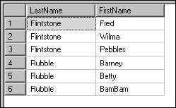
Figure 13-20
Taking this example just one step further, these two functions can be combined into one by passing in a second parameter to indicate the name to extract:
CREATE FUNCTION fnGetName (@FullName VarChar(100)
                         , @FirstOrLast VarChar(5))
RETURNS VarChar(100)
AS
 BEGIN
    DECLARE @CommaPosition Int
    DECLARE @TheName VarChar(100)
    IF @FirstOrLast = ‘First’
       BEGIN
          SET @CommaPosition = CHARINDEX(‘,’, @FullName)
        SET @TheName = SUBSTRING(@FullName, @CommaPosition + 2, LEN(@FullName))
     END
    ELSE IF @FirstOrLast = ‘Last’
       BEGIN
          SET @CommaPosition = CHARINDEX(‘,’, @FullName)
        SET @TheName = SUBSTRING(@FullName, 1, @CommaPosition - 1)
     END
     RETURN @TheName
 END
The new function is called just like before but with the addition of a second parameter, like this:
SELECT dbo.fnFirstName(‘Washington, George’, ‘First’)
Inline Table-Valued Functions
This type of function returns a result set, much like a view. However, unlike a view, functions can accept parameters. The inline function's syntax is quite simple. In the function definition, the return type is set to a Table. A RETURN statement is used with a SELECT query in parentheses:
CREATE FUNCTION fnProductListBySubCategory (@SubCategoryID Int)
 RETURNS Table
AS
 RETURN
 (
    SELECT ProductID, Name, ListPrice FROM Product
    WHERE ProductSubCategoryID = @SubCategoryID
)
The function is treated almost like a table using the syntax Select … From (function name):
SELECT * FROM fnProductListBySubCategory(1)
An added benefit is the ability to process business logic, as you would if using a stored procedure. This example shows the same function as before with an optional parameter and related conditional logic. If a subcategory ID value is provided, products are filtered by this value; otherwise, all products are returned.
CREATE FUNCTION fnProductListBySubCategory (@SubCategoryID Int = Null)
 RETURNS Table
AS
BEGIN
 IF @SubCategoryID Is Null
    BEGIN
      RETURN
        (
        SELECT ProductID, Name, ListPrice
        FROM Product
        )
    END
 ELSE
    BEGIN
      RETURN
        (
        SELECT ProductID, Name, ListPrice
        FROM Product
        WHERE ProductSubCategoryID = @SubCategoryID
        )
    END
  END
For returning a result set from a function, the inline table-valued function is likely the best choice. It's the most elegant blend of SELECT-compatible syntax with stored procedure style input parameters. Aside from these powerful capabilities, the syntax is simple and easy to manage.
Multi-Statement Table-Valued Functions
Multi-statement functions can be used to do some very unique things outside the context of a standard SELECT statement. Like the preceding inline function, this type of function also returns a table-type result set, but the table is explicitly constructed in script. This can be used to accomplish one of two things: either to process some very unique business logic by assembling a virtual table on-the-fly, or to duplicate the functionality of an inline function in a more verbose and complicated way. In short, if you need to select records from an existing table to return a result set, use an inline table-valued function.
The following is an example of the same function demonstrated in the previous section, as a multi-statement function. In the declaration, a table-type variable is used to define the return structure. In this case, the variable @ProdList defines a virtual table with three columns. The fact that these columns are the same as the corresponding columns in the Product table is purely a matter of choice. You can see that in the body of the function, I've inserted rows into the variable as if it were a physical table. Finally, the RETURN statement terminates execution and returns the result set:
CREATE FUNCTION fnProductListBySubCategory (@SubCategoryID Int)
 RETURNS @ProdList Table
    (  ProductID Int
     , Name nVarChar(50)
     , ListPrice Money
    )
AS
 BEGIN
    IF @SubCategoryID IS NULL
      BEGIN
        INSERT INTO @ProdList (ProductID, Name, ListPrice)
       SELECT ProductID, Name, ListPrice
       FROM Product
      END
    ELSE
      BEGIN
        INSERT INTO @ProdList (ProductID, Name, ListPrice)
       SELECT ProductID, Name, ListPrice
       FROM Product
        WHERE ProductSubCategoryID = @SubCategoryID
      END
    RETURN
 END
Now, I'll step out of the mainstream and show you a more unique application for this type of function. This function doesn't select data from a table. The records returned by this function are entirely manufactured within the script contained by the function. The filtering logic, implemented by the @Category parameter, accepts three relevant values: Mainframe, Micro, or All. If the value All is passed, rows for both of the previous categories are returned.
CREATE FUNCTION fnComputerTypes(@Category VarChar(15))
 Returns @CompType Table
    (  Year Int
     , BrandName VarChar(50)
     , ModelName VarChar(50)
     , Category VarChar(25)
    )
 AS
  BEGIN
     IF @Category IN (‘MainFrame’, ‘All’)
       BEGIN
          INSERT INTO @CompType (Year, BrandName, ModelName, Category)
        SELECT 1945, ‘US Ordinance Dept.’, ‘ENIAC’, ‘Mainframe’

          INSERT INTO @CompType (Year, BrandName, ModelName, Category)
         SELECT 1951, ‘Remington Rand’, ‘Univac’, ‘Mainframe’

          INSERT    INTO @CompType (Year, BrandName, ModelName, Category)
          SELECT    1952, ‘IBM’, ‘701’, ‘Mainframe’

          INSERT    INTO @CompType (Year, BrandName, ModelName, Category)
          SELECT    1964, ‘IBM’, ‘System/3 60’, ‘Mainframe’

          INSERT    INTO @CompType (Year, BrandName, ModelName, Category)
          SELECT    1988, ‘IBM’, ‘AS/400’, ‘Mainframe’
       END

    IF @Category    IN (‘Micro’, ‘All’)
       BEGIN
          INSERT    INTO @CompType (Year, BrandName, ModelName, Category)
        SELECT  1977, ‘Tandy Radio Shack’, ‘TSR-80’, ‘Micro’

        INSERT INTO @CompType (Year, BrandName, ModelName, Category)
        SELECT 1981, ‘Commodore ’, ‘VIC-20’, ‘Micro’

        INSERT INTO @CompType (Year, BrandName, ModelName, Category)
        SELECT 1982, ‘Commodore’, ‘Commodore 64’, ‘Micro’

        INSERT INTO @CompType (Year, BrandName, ModelName, Category)
        SELECT 1981, ‘IBM’, ‘PC’, ‘Micro’

        INSERT INTO @CompType (Year, BrandName, ModelName, Category)
        SELECT 2004, ‘Dell’, ‘PowerEdge 1855’, ‘Micro’
        END
    RETURN
  END
I'll test the function using the value All:
SELECT * FROM dbo.fnComputerTypes(‘All’)
The result is shown in Figure 13-21.

As far as the consumer of this data is concerned, it behaves like, and appears to have been selected from, a table in the database.
Transaction Management
You'll recall that in Chapter 9, you learned how to explicitly control transactions. I'll briefly review this topic as it applies to database programming objects. Transaction statements (BEGIN, ROLLBACK, and COMMIT TRANSACTION) are used to queue up a set of statements and control the sequence and dependency of a group of operations. For example, if a stored procedure or user-defined function were to update several sales records and then delete sales records based on some criteria that may have been modified in the UPDATE statement, it would be important to let the update operation finish before deleting any records. In its ever-zealous quest to be efficient, SQL Server may perform operations in parallel, thus working against important business logic. In such cases, it would be important to serialize these dependent operations into separate transactions.
Another important purpose for transactions is to manage the atomicity of a group of operations. If multiple operations are grouped into a single transaction, they are executed as a unit. The outcome of the entire transaction is dependent upon the success of all statements. If they all succeed, the transaction is rolled forward from the transaction log and succeeds. If any operations are unsuccessful, or an error is otherwise raised; the transaction is rolled back, and none of the operations result in committed (inserted, updated, or deleted) records.
Stored procedures are the ideal environment for transactional management. Using the techniques demonstrated in Chapter 9, it's a simple matter to wrap groups of statements into a transactional batch. You can also use error-handling script with transaction management to make your procedures even more bulletproof.
Locking Options
One of the database engine's important jobs is to balance the task of record locking (to protect data as it's modified) and to present consistent result sets of data to queries. This behavior is performed automatically and usually requires no intervention. SQL Server implements locking at various levels based on requested operations and concurrent users sharing the same or adjacent data. On rare occasions, it may be necessary to override the default locking behavior within a transaction. This is done using the SET TRANSACTION ISOLATION LEVEL statement. The locking options described in the following table are supported in SQL Server 2000.
| Locking Option | Description |
| READ UNCOMMITTED | Records are read from the transaction log if they have been modified. This includes “dirty” records that have yet to be rolled forward into table data pages. |
| READ COMMITTED | This is the default behavior. Records are read only from data pages after newly committed rows have been rolled forward into the database. This option prevents inaccurate dirty reads of data within the context of the current transaction. However, concurrent statements could modify records between operations creating an anomaly known as a phantom read. This typically only happens in cases where multiple users are frequently modifying multiple records. |
| REPEATABLE READ | This option locks the transaction unconditionally so that no other operations can modify records. This is an extreme measure that can cause increased locking contention, and is recommended only in rare cases. |
| SERIALIZABLE | This option serializes transactions so that no concurrent operations can be performed that would affect the state of records within the current transaction. This is done by locking records within a range of key values or other search criteria. This has the advantage of simplifying locking contention problems; however, it can impair functionality and performance. |
SQL Server 2005 introduces a new isolation level called SNAPSHOT. Snapshot isolation allows users to access the last committed version of data even if that data is undergoing modification. With Snapshot isolation, when data is modified a copy of the data is written to TempDB. Any other transaction that attempts to read the data being modified will be redirected automatically to the copy stored in TempDB.
The behavior of these options may appear to be easily predictable. However, the actual locking behavior of individual rows, tables, and other objects is a result of the locking options specified by the combined transactions as multiple operations are performed on the same data. The following example serializes these other users' operations on the same data. This way, no modifications would be allowed to these records between the two UPDATE statements:
SET TRANSACTION ISOLATION LEVEL SERIALIZABLE
GO
BEGIN TRANSACTION
GO
    UPDATE Product SET StandardCost = StandardCost * 1.15
    WHERE ProductSubCategoryID = 1
GO
    UPDATE Product SET ListPrice = ListPrice * 1.15
    WHERE ProductSubCategoryID = 1
    AND StandardCost < 1000
GO
COMMIT TRANSACTION
Summary
When designing a database solution, it is important to see the bigger picture. Ideally, queries and other database operations should be contained in manageable database objects. In the long run, views, stored procedures, and user-defined functions provide improved security, performance, and simplicity. In most databases, this is a significant investment and may take time and considerable effort.
Views are SELECT statements that can be treated as a table. By organizing complex queries into views, users and programmers don't have to contend with the complexities of a database design and can focus on their pertinent data and business problems. Federated and partitioned views allow data to be stored on different physical media and in different locations, all of which may be transparent to the consumer.
Stored procedures can simplify common operations, providing a standard approach for managing records and high-level data entities. Complex business logic can be processed in a stored procedure, complete with decision branching and error handling. Stored procedures are reusable objects that run efficiently because the SQL script is compiled and optimized.
User-defined functions can provide the same functionality as views and have a lot of the same capabilities as stored procedures. In some ways, UDFs are the best of both approaches because they support the more common SELECT statement rather than having to be executed like a stored procedure.
Each of these three objects still has its place in SQL programming. Views are far more common than UDFs and under certain conditions may be more efficient. Stored procedures can use nondeterministic functions, which are not allowed in UDFs. The one thing that functions provide that views and procedures do not is the ability to encapsulate the logic to return scalar values. Use UDFs to simplify parsing, calculations, and value manipulation.
Exercises
Exercise 1
Define a new view called vwSalesEmployees. It should return the EmployeeID, FirstName, LastName, and Title columns from the Employee table for all employees who are sales persons. Results should be sorted by last name and then by first name.
Exercise 2
Create a stored procedure called spEmployeeAddUpdate. This procedure accepts three parameters: FirstName, LastName, and LoginID. The data types are nVarChar(50), nVarChar(50), and nVarChar(256), respectively. Define logic in this procedure to check for an existing employee record with the same first and last name values. If the employee record exists, update the LoginID. Otherwise, insert a new employee record.
Exercise 3
Add a comment header block and error handling logic to the procedure you created in exercise 2. The block should contain a description of the procedure, parameters, your contact information, the date created, and revision information.
Add error-handling logic to catch the errors that would occur if a parameter were omitted or if a null value were passed into a parameter. If an error is caught, raise a custom error message.
Exercise 4
If you have completed all previous exercises, use the following script to produce a message. Analyze each statement so you understand how each value is produced.
USE AdventureWorks2000
GO
--
ALTER FUNCTION dbo.fnProperCase (@In VarChar(255))
   RETURNS VarChar(255)
AS
BEGIN
   RETURN UPPER(SUBSTRING(@In, 1, 1)) + LOWER(SUBSTRING(@In, 2, 254))
END
GO
-- Execute query from here if function has already been created --
-- Assemble message from string fragments:
DECLARE @Message VarChar(255)
SELECT @Message = dbo.fnProperCase(REVERSE(SUBSTRING(LastName, 4, 3))) FROM
Employee WHERE EmployeeID = 199
SET @Message = @Message + ‘ ’ + CHAR(73) + CHAR(3 9) + CHAR(109) + ‘ ’ + CHAR(97)
SELECT @Message = @Message + ‘ ’ + dbo.fnProperCase(SUBSTRING(Description, 61, 5))
FROM ProductDescription WHERE ProductDescriptionID = 1586
SELECT @Message = @Message + SUBSTRING(Name, 6, 3) FROM ProductSubCategory WHERE
ProductSubCategoryID = 38
SELECT @Message = @Message + CHAR(45) + SUBSTRING(@@SERVICENAME, 3, 3)
SELECT @Message = @Message + ‘ ’ + LOWER(SUBSTRING(Description, 1, 3)) FROM
ProductDescription WHERE ProductDescriptionID = 847
SELECT @Message = @Message + SUBSTRING(LastName, 4, 3) FROM Employee WHERE
EmployeeID = 21
SELECT @Message = @Message + CHAR(33)
-- Print the entire string:
PRINT @Message