
6
SQL Functions
Now that you understand how to formulate SQL queries and return result sets, you need to do something useful with this data. Once you have successfully retrieved values from tables, it's very common to further manipulate values to provide useful and meaningful results. This may involve the following:
- Performing calculations and mathematical operations
- Conversion
- Parsing
- Combining values
- Aggregation
The purpose of this chapter is to help you learn the mechanics of using functions of all kinds. It introduces you to some of the more common value manipulation functions and some less-common functions to give a sample of these powerful capabilities. You'll also take a look at some new functionality offered in SQL Server 2005.
At the end of the book, you'll find a reference for all of the system-supplied functions and the syntax needed to use them. Additionally, subsequent chapters contain more detailed information about specific groups of functions. For example, Chapter 7 discusses specific uses for aggregate functions in more advanced SQL queries, and Chapter 11 shows you how to use functions to support full-text index searches.
Transact-SQL functions are grouped into the categories described in the following table.
The Anatomy of a Function
The purpose of a function is to return a value. Most of the functions you will use return a scalar value, meaning a single unit of data, or a simple value. However, functions can return practically any data type, and this includes types such as Table and Cursor, which could be used to return entire, multi-row result sets. I won't take the discussion to that level in this chapter. Chapter 13 explains how to create and utilize user-defined functions to return more complex data.
Functions have been around for a long time, even long before SQL. The pattern used to call functions is the same in nearly all programming languages:
In Transact-SQL, values are returned using the SELECT statement. If you just want to return a value in a query, you treat the SELECT as the output operator without using an equals sign:
I'd Like to Have an Argument
When it comes to SQL functions, the term argument is used to mean an input variable or placeholder for a value. Functions can have any number of arguments and some arguments are required whereas others are optional. Optional arguments are typically at the end of the comma-delimited argument list, making them easier to exclude if they are not to be provided in the function call.
When you read about functions in SQL Server Books Online or on-line help, you'll see optional arguments denoted in square brackets. In this example for the CONVERT() function, both the length argument for the data type and the style argument for the CONVERT() function are optional:
I'll simplify this because we're really not discussing how to use data types at the moment:
According to this, the CONVERT() function will accept either two or three arguments. So, either of these examples would be acceptable:
SELECT CONVERT(VarChar(20), ‘April 29, 1988’)

SELECT CONVERT(VarChar(20), ‘April 29, 1988’, 101)
The first argument for this function is the data type, VarChar(20), and the second argument is the value, ‘April 29, 1988’. The third argument in the second statement determines the style for numeric and date types. Even if a function doesn't take an argument, or doesn't require an argument, it is called with a set of empty parentheses. Note that when a function is referred to by name throughout the book, the parentheses are included because this is considered standard form.
Deterministic Functions
Because of the inner-workings of the database engine, SQL Server has to separate functions into two different groups based on what's called determinism. This is not a new-age religion. It's simply a statement about whether the outcome of a function can be predicted based on its input parameters or by executing it one time. If a function's output is not dependent on any external factors, other than the value of input parameters, it is considered to be a deterministic function. If the output can vary based on any conditions in the environment or algorithms that produce random or dependent results, the function is non-deterministic. Why make a big deal about something that seems so simple? Well, nondeterministic functions and global variables can't be used in some database programming objects such as user-defined functions. This is partially due to the way SQL Server caches and precompiles executable objects. For simple, ad-hoc queries, knock yourself out and use any type of function you like, but if you plan on building more advanced, reusable programming objects, it's important to understand this distinction. As a brief example, these functions are deterministic:
- AVG() (all aggregate functions are deterministic)
- CAST()
- CONVERT()
- DATEADD()
- DATEDIFF()
- ASCII()
- CHAR()
- SUBSTRING()
These functions and variables are nondeterministic:
- GETDATE()
- @@ERROR
- @@SERVICENAME
- CURSORSTATUS()
- RAND()
You can find a complete list of all functions and their determinism in Appendix B.
Using Variables with Functions
Variables can be used for both input and output. In Transact-SQL, a variable is prefixed with the @ symbol, declared as a specific data type, and can then be assigned a value using either the SET or SELECT statements. The following example shows the use of an Int type variable called @MyNumber, passed to the SQRT() function:
DECLARE @MyNumber Int
SET @MyNumber = 144
SELECT SQRT(@MyNumber)
The result of this call is 12, the square root of 144.
Using SET to Assign Variables
The following example uses another Int type variable, @MyResult, to capture the return value for the same function. This technique is most like the pattern used in procedural programming languages:
DECLARE @MyNumber Int, @MyResult Int
SET @MyNumber = 144

-- Assign the function result to the variable:
SET @MyResult = SQRT(@MyNumber)
-- Return the variable value
SELECT @MyResult
Using SELECT to Assign Variables
The same result can be achieved using a variation of the SELECT statement. A variable is declared prior to assigning a value. The chief advantage of using the SELECT statement instead of the SET command is that multiple variables can be assigned values in a single operation. The value is assigned using the SELECT statement and then can be used for any purpose after this script has been executed:
DECLARE @MyNumber1 Int, @MyNumber2 Int, @MyResult1 Int, @MyResult2 Int
SELECT @MyNumber1 = 144, @MyNumber2 = 121
-- Assign the function result to the variable:
SELECT @MyResult1 = SQRT(@MyNumber1), @MyResult2 = SQRT(@MyNumber2)
-- Return the variable value
SELECT @MyResult1, @MyResult2
Functionally, these techniques are identical; however, populating multiple variables with a SELECT statement is a great deal more efficient in regards to server resources than multiple SET commands. The limitation of selecting multiple or even single values into parameters is that the population of variables cannot be combined with data retrieval operations. This is why the preceding example used a SELECT statement to populate the variables followed by a second SELECT statement to retrieve the data in the variables. For example, the following script will not work:
DECLARE @ContactName VarChar(65)
SELECT @ContactName = FirstName + ‘ ’ + LastName, Phone
FROM Contact WHERE ContactID = 3
This script will generate the following error:
Msg 141, Level 15, State 1, Line 2
A SELECT statement that assigns a value to a variable must not be combined with
data-retrieval operations.
Using Functions in Queries
Functions are often combined with query expressions to modify column values. This is easily done by passing column names to function arguments. The function reference is inserted into the column list of a SELECT query, like this:
SELECT FirstName, LastName, YEAR(BirthDate) AS BirthYear
FROM Employee
In this example, the BirthDate column value is passed into the YEAR() function as an argument. The function's result becomes the aliased column BirthYear.
Nested Functions
Often, you will find that the functionality you need doesn't exist in a single function. By design, functions are intended to be simple and focused on providing a specific feature. If functions did a lot of different things, they would be complicated and difficult to use (and some are, but fortunately, not many). For this and other reasons, each function simply does one thing. To get all of the functionality I need, I may pass the value returned from one function into another function. This is known as a nested function call. Here's a simple example: The purpose of the GETDATE() function is to return the current date and time. It doesn't return elegantly formatted output; that's the job of the CONVERT() function. To get the benefit of both functions, I pass the output from the GETDATE() function into the value argument of the CONVERT() function, like this:
SELECT CONVERT(VarChar(20), GETDATE(), 101)
You'll see a few examples of this pattern throughout this chapter.
Aggregate Functions
The essence of reporting is typically to distill a population of data into a value or values representing a trend or summary. This is what aggregation is all about. Aggregate functions answer the questions asked by the consumers of data:
- “What were the total sales of chicken gizzard by-products for last month?“
- “What is the average price paid for food condiments by male Brazilians between the ages of 19 and 24?”
- “What was the longest order-to-shipping time of all orders last quarter?”
- “Who is the oldest employee still working in the mail room?”
Aggregate functions return a scalar value (a single value) applying a specific aggregate operation. The return data type is comparable to that of the column or value passed to the function. Aggregates are often used along with grouping, rollup, and pivoting operations to produce results for data analysis. This is covered in greater detail in Chapter 7. The focus here is on some of the more common functions in simple SELECT queries.
Aggregate functions can be used with scalar input values, rather than in a SELECT query, but what's the point? I can pass the value 15 to each of these aggregate functions and each will return the same result:
SELECT AVG(15)

SELECT SUM(15)

SELECT MIN(15)

SELECT MAX(15)
They all return 15. After all, the average, sum, smallest, and largest value in a range of one value is that value. What happens if I count one value?
I get 1. I counted one value.
All right, now let's do something useful. Aggregate functions are really only valuable when used with a range of values in a result set. Each function performs its magic on all non-null values of a column. Unless you are applying grouping (which you will see in Chapter 7) you cannot return both aggregated values and regular column values in the same SELECT statement.
AVG()
The AVG() function returns the average for a range of numeric values, for all non-null values. For example, a table contains the following gymnastics meet scores:
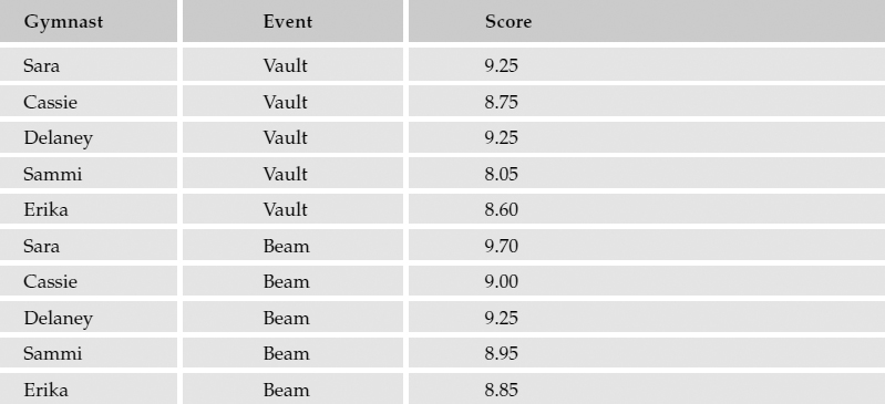
The following query is executed with these values:
SELECT AVG(Score)
The result would be 8.965.
If three girls didn't compete in some events and the table had some missing scores, these might be represented as NULLs:
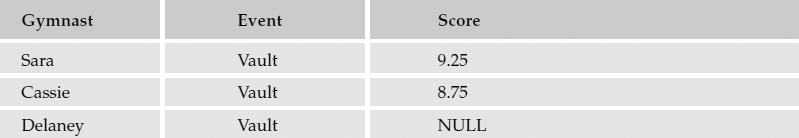
In this case, the NULL values are not considered, and the average is calculated based on the existing numerical values. The result would be 8.921429.
However, if the missing scores were counted against the team, and the column contained zero values instead, this would seriously affect the overall score (6.245) and their chances of moving on to state competition.
COUNT()
The COUNT() function returns an integer value for the number of non-null values in the column range. For instance, if the gymnastics data in the previous example were in a table called GymEvent and I wanted to know the number of events that Sammi received a score on, I could execute the following query:
SELECT COUNT(Score) FROM GymEvent WHERE Gymnast = ‘Sammi’
The result would be 1 since the score for Sammi's Beam event was NULL. If you need a count of all rows in a table, regardless of NULL values, use the following syntax:
SELECT COUNT(*) FROM table
Using the previous example with Sammi, a COUNT(*) query would look like this:
SELECT COUNT(*) FROM GymEvent WHERE Gymnast = ‘Sammi’
Because the COUNT(*) function ignores NULL values, the result of this query would be 2.
MIN() and MAX()
The MIN() function returns the smallest (minimum) non-null value for a column range. The MAX() function returns the maximum or largest value. These functions can be used with most data types and work according to the sorting rules of the type. To make this point, suppose a table contains the following values stored in two different columns, one as an integer type and the other as a character type:
| Column1 (Int type) |
Column2 (VarChar type) |
| 2 | 2 |
| 4 | 4 |
| 12 | 12 |
| 19 | 19 |
What will the MIN() and MAX() functions return? You may be surprised.

Because values in Column2 are stored as characters rather than numbers, it is sorted according to the ASCII value of each character, from left to right. This is why 12 is less than any other value and 4 is greater than any other value.
SUM()
The SUM() function is one of the most commonly used aggregates and is fairly self-explanatory. Like the AVG() function, it works with numeric data types and returns the additive sum of all non-null values in a column range.
You'll learn to use all of the aggregate functions in Chapter 7, including statistical functions. You'll also see how to create user-defined aggregates with SQL Server 2005.
Configuration Variables
These aren't really functions but they can be used in much the same way as system functions. Each global variable returns scalar information about the SQL Server execution environment. Following are some common examples.
@@ERROR
This variable contains the last error number for the current connection. The default value for @@ERROR is zero. Errors are raised by the database engine when standard error conditions occur. All of the standard error numbers and messages are stored in the sysmessages table and can be queried using the following script:
Custom errors can be raised manually using the RAISERROR statement and can be added to the sysmessages table using the sp_addmessage system stored procedure.
Following is a simple example of the @@ERROR variable. First I try to divide a number by zero. This causes the database engine to raise the standard error number 8134.
SELECT 5 / 0
SELECT @@ERROR
Successfully retrieving the value of @@ERROR causes the value of @@ERROR to return to zero. This because @@ERROR only holds the error number for the previously executed statement. If I want to retrieve additional error information, I can get it from the sysmessages table (or view it in SQL Server 2005) using the following script:
SELECT 5 / 0

SELECT * FROM master.dbo.sysmessages WHERE error = @@ERROR
Executing this script returns more detailed error information from the sysmessages table shown in Figure 6-1.
Figure 6-1
If I had installed SQL Server with languages in addition to U.S. English, additional messages would be listed. Each language-specific error message has a language identifier (mslangid), which corresponds to a language in the syslanguages table.
@@SERVICENAME
This is the name of the Windows service used to execute and maintain the current instance of SQL Server. This will typically return the value MSSQLSERVER. Non-default instances (if you were to install SQL Server more than once or choose to install it as a named instance) have uniquely named service names.
@@TOTAL_ERRORS
This is the total number of errors that have occurred since the current connection was opened. Like the @@ERROR variable, this is unique for each user session and is reset when each connection closes.
@@TOTAL_READ
This is a count of the total read operations that have occurred since the current connection was opened.
@@VERSION
This variable contains the complete version information for the current instance of SQL Server.
SELECT @@VERSION
For example, for an instance of SQL Server 2000, this script returns the following:
The actual version number, used internally at Microsoft, is a simple integer value, although released products may have other branded names. In this case, SQL Server 2000 is really version 8. Windows XP Professional shows up as Windows NT version 5.1. The build number is used for internal control and reflects changes made in beta and preview product releases, and post-release service packs. Here is an example of the output for SQL Server 2005 running on Windows Server 2003:
Microsoft SQL Server 2005 - 9.00.1090 (Intel X86)
  Feb 21 2005 03:39:52
  Copyright (c) 1988-2004 Microsoft Corporation
  Enterprise Edition on Windows NT 5.2 (Build 3790: )
Conversion Functions
Data type conversion can be performed using the CAST() and CONVERT() functions. For most purposes, these two functions are redundant and reflect the evolutionary history of the SQL language. The functionality may be similar, however the syntax is different. Not all values can be converted to other data types. Generally speaking, any value that can be converted can be done so with a simple function call.
CAST()
The CAST() function accepts one argument, an expression, which includes both the source value and a target data type separated by the word AS. Here is an example, using the literal string ‘123’ converted to an integer:
SELECT CAST(‘123’ AS Int)
The return value will be the integer value 123. However, what happens if you try to convert a string representing a fractional value to an integer?
SELECT CAST(‘123.4’ AS Int)
Neither the CAST() nor the CONVERT() functions will do any guessing, rounding, or truncation for you. Because the value 123.4 can't be represented using the Int data type, the function call produces an error:
Server: Msg 245, Level 16, State 1, Line 1
Syntax error converting the varchar value ‘123.4’ to a column of data type int.
If you need to return a valid numeric equivalent value, you must use a data type equipped to handle the value. There are a few that would work in this case. If you use the CAST() function with your value to a target type of Decimal, you can specifically define the precision and scale for the decimal value. In this example, the precision and scale are 9 and 2, respectively. Precision is the total number of digits that can be stored to both the left and right of the decimal point. Scale is the number of digits that will be stored to the right of the decimal point. This means that the maximum whole number value would be 9,999,999 and the smallest fractional number would be .01.
SELECT CAST(‘123.4’ AS Decimal(9,2))
The Decimal data type displays the significant decimal positions in the results grid:
The default values for precision and scale are 18 and 0 respectively. Without providing values for precision and scale of the Decimal type, SQL Server effectively truncates the fractional part of the number without causing an error.
SELECT CAST(‘123.4’ AS Decimal)
The result looks like an integer value:
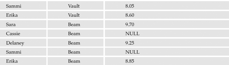
Applying data type conversions to table data is very easy to do. The next example uses the Employee table, and starts with the following query:
SELECT FirstName, LastName, DepartmentID, ShiftID, BirthDate
FROM Employee
ORDER BY LastName
Ordering by the last name just gives you some variety in the DepartmentID and ShiftID column values in the first page of the results grid. The results are shown in Figure 6-2.
You'd like to create a new value, made up of the DepartmentID and ShiftID separated by a hyphen. If you use the following expression, you don't get the result you're looking for. In fact, the hyphen isn't even included in the resulting value.
SELECT DepartmentID + ‘-’ + ShiftID FROM Employee
The problem with this expression is that you're trying to concatenate an integer (the DepartmentID), a character value (the hyphen), and another integer (the ShiftID). Apparently, the query engine perceives the hyphen to be a mathematical operator, rather than a character. Regardless of the outcome, you need to fix the expression and make sure you are working with the appropriate data types. This expression makes the necessary type conversions:
SELECT CAST(DepartmentID AS VarChar(5)) + ‘-’ + CAST(ShiftID AS VarChar(5))
ROM Employee
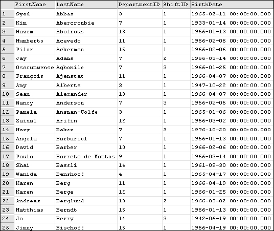
Figure 6-2
Converting the integer values to the VarChar type makes these character values without adding any extra spaces. These values are combined with the hyphen using the plus sign to concatenate string values rather than adding and subtracting the previous numeric values. Now add the first name, last name, and birth date columns:
SELECT FirstName
     , LastName
     , CAST(DepartmentID AS VarChar(5)) + ‘-’ + CAST(ShiftID AS VarChar(5): AS DS
     , BirthDate
FROM Employee
ORDER BY LastName
The results are shown in Figure 6-3.
Don't worry about the BirthDate column. I have plans for it in the next section. As you see, the DepartmentID and ShiftID are combined as you wanted them to be.
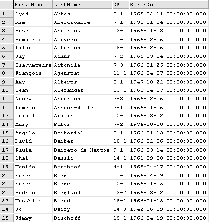
Figure 6-3
CONVERT()
For simple type conversion, the CONVERT() function does the same thing as the CAST() function, only with different syntax. It requires two arguments: the first for the target data type and the second for the source value. Here are a couple of quick examples similar to those used in the preceding section:
SELECT CONVERT(INT, ‘123’)

SELECT CONVERT(Decimal(9,2), ‘123.4’)
The CONVERT() function also has some enhanced features making it useful for returning formatted string values. Date values can be formatted in a variety of ways. There are 28 predefined date formats to accommodate international and special-purpose date and time output. The following table shows how these break down.
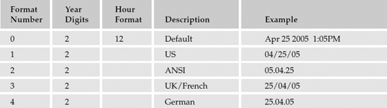
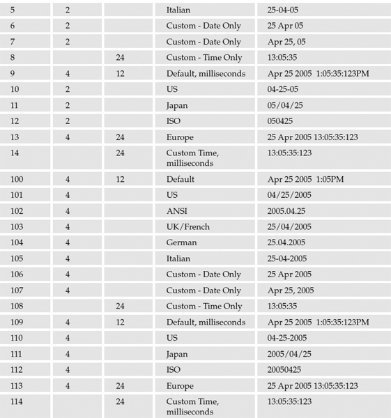
The third argument to this function is optional and accepts the format number integer value. The examples provided in the grid apply to the DateTime data type. When converting from the SmallDateTime data type, the formatting remains the same but some elements will display 0. Here are a few examples of some related script along with formatted date output:
SELECT ‘Default Date: ’ + CONVERT(VarChar(50), GETDATE(), 100)Default Date: Apr 25 2005 1:05PM
SELECT ‘US Date: ’ + C0NVERT(VarChar(50), GETDATE(), 101)US Date: 04/25/2005
SELECT ‘ANSI Date: ’ + C0NVERT(VarChar(50), GETDATE(), 102)ANSI Date: 2005.04.25
SELECT ‘UK/French Date: ’ + C0NVERT(VarChar(50), GETDATE(), 103)UK/French Date: 25/04/2005
SELECT ‘German Date: ’ + C0NVERT(VarChar(50), GETDATE(), 104)German Date: 25.04.2005
Format numbers 0, 1, and 2 also apply to numeric types and affect the format of decimal and thousand separators. The effect is different for different data types. In general, using the format number 0 (or no value for this argument) returns a formatted value in the data type's most native form. Using 1 or 2 generally displays a more detailed or precise value. The following example uses 0:
DECLARE @Num Money
SET @Num = 1234.56
SELECT C0NVERT(VarChar(50), @Num, 0)
It returns the following:
Using 1 returns the following:
And using 2 returns the following:
This example does the same thing with a Float type:
DECLARE @Num Float
SET @Num = 1234.56
SELECT C0NVERT(VarChar(50), @Num, 2)
Using the value 0 doesn't change the format from what you've provided but using 1 or 2 returns the number expressed in scientific notation, the latter using 15 decimal positions:
The STR() Function
This is a quick-and-easy conversion function that converts a numeric value to a string. The function accepts three arguments: the numeric value, the overall length, and the number of decimal positions. If the integer part of the number and decimal positions is shorter than the overall length, the result is left-padded with spaces. In this first example, the value (including the decimal) is five characters long. I've made it a point to show the results in the grid so you can see any left padding. This call asks for an overall length of eight characters with four decimal positions:
SELECT STR(123.4, 8, 4)
The result has the decimal value right-filled with 0s, as shown in Figure 6-4.
Figure 6-4
Here I'm passing in a ten-character value and asking for an eight-character result, with four decimal positions:
SELECT STR(123.456789, 8, 4)
The result must be truncated to meet my requirements. The STR() function rounds the last digit, as shown in Figure 6-5.
Figure 6-5
Now I'll pass in the number 1 for the value and ask for a six-character result with four decimal positions. In this case, the STR() function right-fills the decimal value with zeros, as shown in Figure 6-6.
SELECT STR(1, 6, 4)
Figure 6-6
However, if I specify an overall length greater than the length of the value, decimal point, and the decimal value, the result will be left-padded with spaces, as shown in Figure 6-7.
SELECT STR(1, 12, 4)
Figure 6-7
Cursor Functions and Variables
Chapter 10 discusses the use of cursors along with some of the pros and cons of using this technique. The short version of this topic is that cursors can provide the ability to process multiple rows of data, one row at a time, in a procedural loop. This ability comes at a cost when compared with more efficient, set-based operations. One function and two global variables are provided to help manage cursor operations.
The CURSOR_STATUS() Function
This function returns an integer indicating the status of a cursor-type variable passed into the function. A number of different types of cursors can affect the behavior of this function. For simplicity, the return value will typically be one of those listed in the following table.
| Return Value | Description |
| 1 | Cursor contains one or more rows (dynamic cursor contains 0 or more rows) |
| 0 | Cursor contains no rows |
| -1 | Cursor is closed |
| -2 | Cursor is not allocated |
| -3 | Cursor doesn't exist |
@@CURSOR_ROWS
This variable is an integer value representing the number of rows in the cursor open in the current connection. Depending on the cursor type, this value may or may not represent the actual number of rows in the result set.
@@FETCH_STATUS
This variable is a flag that indicates the state of the current cursor pointer. It is used primarily to determine whether a row still exists and when you have reached the end of the result set after executing a FETCH NEXT statement.
Date Functions
These functions are used for working with DateTime and SmallDateTime type values. Some are used for parsing the date and time portions of a date value and for comparing and manipulating date/time values.
The DATEADD() Function
The DATEADD() function adds a specific number of date unit intervals to a date/time value. For example, to determine the date 90 days after April 29, 1988, the following statement is used:
SELECT DATEADD(Day, 90, ‘4-29-1988’)
The answer is as follows:
Any of the values in the following table can be passed in the Interval argument.
| Interval | Interval Argument Values |
| Year | Year, yyyy, yy |
| Quarter | quarter, qq, q |
| Month | Month, mm, m |
| Day of the year | dayofyear, dy, y |
| Day | Day, dd, d |
| Week | Week, wk, ww |
| Hour | Hour, hh |
| Minute | minute, mi, n |
| Second | second, ss, s |
| Millisecond | millisecond, ms |
Using the same date as before, here are some more examples. This time, I'll include the time as well. The results are on the following line:
18 years later:
SELECT DATEADD(year, 18, ‘4-29-1988 10:30 AM’)2006-04-29 10:30:00.000
18 years before:
SELECT DATEADD(yy, -18, ‘4-29-1988 10:30 AM’)1970-04-29 10:30:00.000
9,000 seconds after:
SELECT DATEADD(second, 9000, ‘4-29-1988 10:30 AM’)1988-04-29 13:00:00.000
9,000,000 milliseconds before:
SELECT DATEADD(mi, -9000000, ‘4-29-1988 10:30 AM’)1971-03-20 10:30:00.000
I can combine the CONVERT()and the DATEADD() functions to format a return date value nine months before September 8, 1989:
SELECT C0NVERT(VarChar(20), DATEADD(m, -9, ‘9-8-1989’), 101)12/08/1988
This returns a variable-length character value, a little easier to read than the default dates you saw in the previous results. This is a nested function call where the results from the DATEADD() function (a DateTime type value) are fed to the value argument of the CONVERT() function.
The DATEDIFF() Function
I think of the DATEADD() and DATEDIFF() functions as cousins — sort of like multiplication and division. There are four elements in this equation: the start date, the interval (date unit), the difference value, and the end date. If you have three, you can always figure out what the fourth one is. I use a start date, an integer value, and interval unit with the DATEADD() function to return the end date value relative to a starting date. The DATEDIFF() function returns the difference integer value if I provide the start and end dates and interval. Do you see the relationship?
To demonstrate, I simply choose any two dates and an interval unit as arguments. The function returns the difference between the two dates in the interval unit provided. I want to know what the difference is between the dates 9-8-1989 and 10-17-1991 in months:
SELECT DATEDIFF(month, ‘9-8-1989’, ‘10-17-1991’)
The answer is 25 months. How about the difference in days?
SELECT DATEDIFF(day, ‘9-8-1989’, ‘10-17-1991’)
It's 769 days.
How about the difference in weeks between 7-2-1996 and 8-4-1997?
SELECT DATEDIFF(week, ‘7-2-1996’, ‘8-4-1997’)
57 weeks.
You can even figure out how old you are in seconds:
DECLARE @MyBirthDate DateTime
SET @MyBirthDate = ‘3-24-1967’
SELECT DATEDIFF(ss, @MyBirthDate, GETDATE())
Someone is over 1.3 billion seconds old!
I apply this function to a query by passing a column name to the value argument. This will tell me the approximate age of each employee:
SELECT FirstName, LastName, DATEDIFF(year, BirthDate, GETDATE())
FROM Employee
Figure 6-8 shows the first 25 rows in the results.
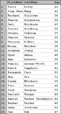
Figure 6-8
This may look right at first glance, but it's not accurate to the day. For example, according to the database, Brian Welker's birth date is on July 8 and he would be celebrating his 38th birthday this year (I'm running the query in April). If I were to use the previous calculation to determine when his age changes, I would be sending Brian a birthday card sometime in January, about six months early.
Unless you find the difference between these dates in a more granular unit and then do the math, the result will only be accurate within a year of the employee's actual birth date. This example factors the number of days in a year (including leap year). Converting to an Int type truncates, rather than rounds, the value:
SELECT FirstName, LastName
, CONVERT(Int, DATEDIFF(day, BirthDate, GETDATE())/365.25) As Age
FROM Employee
Compare the results shown in Figure 6-9 with those of the previous example.
Now Brian is 37 and the rest of the employees' ages should be accurate within a day. The BirthDate column in this table stores the employee's birth date as of midnight (00:00:00 AM). This is the first second of a date. The GETDATE() function returns the current date and time. This means that I'm comparing a two dates with a difference of about eight hours (it's about 8:00 AM as I write this). If you want this calculation to be even more accurate, you need to convert the result of the GETDATE() function to a DateTime value at midnight of the current date.
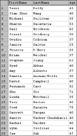
Figure 6-9
The DATEPART() and DATENAME() Functions
These functions return the date part, or unit, for a DateTime or ShortDateTime value. The DATEPART() function returns an integer value and the DATENAME() function returns a string containing the descriptive name, if applicable. For example, passing the date 4-29-1988 to the DATEPART() function and requesting the month returns the number 4:
SELECT DATEPART(month, ‘4-29-1988’)
Whereas, with the same parameters, the DATENAME() function returns April:
SELECT DATENAME(month, ‘4-29-1988’)
Both of these functions accept values from the same list of date part argument constants as the DATEADD() function.
The GETDATE() and GETUTCDATE() Functions
Both of these functions return the current date and time as a DateTime type. The GETUTCDATE() function uses the time zone setting on the server to determine the equivalent Universal Time Coordinate time. This is the same as Greenwich Mean Time or what pilots call “Zulu Time.” Both functions are accurate to 3.33 milliseconds:
SELECT GETDATE()
SELECT GETUTCDATE()
Executing these functions returns the unformatted result shown in Figure 6-10.
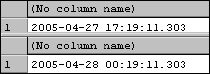
Figure 6-10
Because I'm in the Pacific time zone, there is a seven-hour difference between the current time and UTC. I can verify this using the following DATEDIFF() function call:
SELECT DATEDIFF(hour, GETDATE(), GETUTCDATE())
The DAY(), MONTH(), and YEAR() Functions
These three functions return an integer date part of a DateTime or SmallDateTime type value. They serve a variety of useful purposes including the ability to create your own unique date formats. Suppose I need to create a custom date value as a character string. By converting the output from each of these functions to character types and then concatenating the results, I can arrange them practically any way I want:
SELECT ‘Year: ’ + CONVERT(VarChar(4), YEAR(GETDATE()))
   + ‘, Month: ’ + CONVERT(VarChar(2), MONTH(GETDATE()))
   + ‘, Day: ’ + CONVERT(VarChar(2), DAY(GETDATE()))
This script produces the following:
The next section discusses string manipulation functions and uses a similar technique to build a compact custom time stamp.
String Manipulation Functions
String functions are used to parse, replace, and manipulate character values. One of the great challenges when working with quantities or raw character data is to reliably extract meaningful information. A number of string parsing functions are available to identify and parse substrings (a portion of a larger character type value). As humans, we do this all the time. When presented with a document, an invoice, or written text, we intuitively identify and isolate the meaningful pieces of information. To automate this process can be a cumbersome task when dealing with even moderately complex text values. These functions contain practically all of the tools necessary. The challenge is to find the simplest and most elegant method.
The ASCII(), CHAR(), UNICODE(), and NCHAR() Functions
These four functions are similar because they all deal with converting values between a character and the industry standard numeric representation of a character. The American Standard Code for Information Interchange (ASCII) standard character-set includes 128 alpha, numeric, and punctuation characters. This set of values is the foundation of the IBM PC architecture, and although some of it is now somewhat antiquated, much remains and is still central to modern computing. If you use the English language on your computer, every character on your keyboard is represented in the ASCII character-set. This is great for English-speaking (or at least English typing) computer users, but what about everyone else on the planet?
In the evolution of the computer, it didn't take long for the ASCII set to become obsolete. It was soon extended to form the 256-character ANSI character-set which uses a single byte to store every character. Still an American standard (held by the American National Standards Institute), this extended list of characters meets the needs of many other users, supporting mainly European language characters, but is still founded on the original English-language character-set. To support all printable languages, the Unicode standard was devised to support multiple, language-specific character-sets. Each Unicode character requires 2 bytes of storage space, twice the space as ASCII and ANSI characters, but with 2 bytes more than 65,000 unique characters can be represented. SQL Server supports both ASCII and Unicode standards.
The two ASCII-based functions are ASCII() and CHAR().The fundamental principle here is that every character used on the computer is actually represented as a number. To find out what number is used for a character, pass a single-character string to the ASCII() function:
SELECT ASCII(‘A’)
This returns 65.
What if I know the number and want to convert it to a character? That's the job of the CHAR() function:
SELECT CHAR(65)
This returns the letter A.
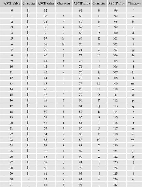
To get a complete list of ASCII character values, I can populate a temporary table with the values 0 through 127 and then use the CHAR() function to return the corresponding characters. I'll shorten the script but include the entire result set in multi-column format, to save space:
-- Create temporary table for numbers:
Create Table #ASCIIVals (ASCIIValue SmallInt)

-- Insert numbers 0 - 127 into table:
Insert Into #ASCIIVals (ASCIIValue) Select 0
Insert Into #ASCIIVals (ASCIIValue) Select 1
Insert Into #ASCIIVals (ASCIIValue) Select 2
Insert Into #ASCIIVals (ASCIIValue) Select 3
Insert Into #ASCIIVals (ASCIIValue) Select 4
…
Insert Into #ASCIIVals (ASCIIValue) Select 123
Insert Into #ASCIIVals (ASCIIValue) Select 124
Insert Into #ASCIIVals (ASCIIValue) Select 125
Insert Into #ASCIIVals (ASCIIValue) Select 126
Insert Into #ASCIIVals (ASCIIValue) Select 127

-- Return all integer values and corresponding ASCII characters:
SELECT ASCIIValue, CHAR(ASCIIValue) As Character FROM #ASCIIVals
Here are the results reformatted in a multi-column grid. Note that non-printable control characters show as small squares in the results grid. Depending on a number of factors, such as fonts or languages installed, these may be displayed a little differently.
The UNICODE() function is the Unicode equivalent of the ASCII() function, and the NCHAR() function does the same thing as the CHAR() function only with Unicode characters. SQL Server's nChar and nVarChar types will store any Unicode character and will work with this function. For extremely large values, the nText type and the new nChar(max) and nVarChar(max) types in SQL Server 2005 also support Unicode characters.
To return extended characters, I'll execute the NCHAR() function with sample character codes:
SELECT NCHAR(220)
This returns the German U umlaut, Ü.
SELECT NCHAR(233)
This returns an accented lowercase e, é.
SELECT NCHAR(241)
This returns a Spanish “enya,” or n with a tilde, ñ.
The CHARINDEX() and PATINDEX() Functions
CHARINDEX() is the original SQL function used to find the first occurrence of a substring within another string. As the name suggests, it simply returns an integer that represents the index of the first character of the substring within the entire string. The following script looks for an occurrence of the string ‘sh’ within the string ‘Washington’:
SELECT CHARINDEX(‘sh’, ‘Washington’)
This returns 3 to indicate that the ‘s’ is the third character in the string ‘Washington’. Using two characters for the substring wasn't particularly useful in this example but could be if the string contained more than one letter s.
The PATINDEX() function is the CHARINDEX() function on steroids. It will perform the same task in a slightly different way, but has the added benefit of supporting wildcard characters (such as those you would use with the Like operator). As its name suggests, it will return the index of a pattern of characters. This function also works with large character types such as nText, nChar(max), and nVarChar(max). Note that if PATINDEX() is used with these large data types, it returns a BigInt type rather than an Int type. Here's an example:
SELECT PATINDEX(‘%M_rs%’, ‘The stars near Mars are far from ours’)
Note that both percent characters are required if you want to find a string with zero or more characters before and after the string being compared. The underscore indicates that the character in this position is not matched. The string could contain any character at this position.
Compare this to the CHARINDEX() function used with the same set of strings:
SELECT CHARINDEX(‘Mars’, ‘The stars near Mars are far from ours’)
Both of these functions return the index value 16. Remember how these functions work. I'll combine this with the SUBSTRING() function in the following section to demonstrate how to parse strings using delimiting characters.
The LEN() Function
The LEN() function returns the length of a string as an integer. This is a simple but useful function that is often used alongside other functions to apply business rules. The following example tests the Month and Day date parts integers, converted to character types, for their length. If just one character is returned, it pads the character with a zero and then assembles an eight-character date string in US format (MMDDYYYY):
DECLARE @MonthChar VarChar(2), @DayChar VarChar(2), @DateOut Char(8)

SET @MonthChar = CAST(MONTH(GETDATE()) AS VarChar(2))
SET @DayChar = CAST(DAY(GETDATE()) AS VarChar(2))

-- Make sure month and day are two char long:
IF LEN(@MonthChar) = 1
 SET @MonthChar = ‘0’ + @MonthChar
IF LEN(@DayChar) = 1
 SET @DayChar = ‘0’ + @DayChar

-- Build date string:
SET @DateOut = @MonthChar + @DayChar + CAST(YEAR(GETDATE()) AS Char(4))

SELECT @DateOut
The return value from this script will always be an eight-character value representing the date:
The LEFT() and RIGHT() Functions
The LEFT() and RIGHT() functions are similar in that they both return a substring of a specified size. The difference between the two is what part of the character string is returned. The LEFT() function returns characters from the left-most part of the string, counting characters to the right. The RIGHT() function does exactly the opposite. It starts at the right-most character and counts to the left, returning the specified number of characters. Take a look at an example that uses the string ‘George Washington’ to return substrings using these functions.
If I ask to return a five-character substring using the LEFT() function, the function locates the left-most character, counts five characters to the right, and returns the substring shown in Figure 6-11.
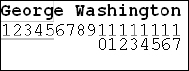
Figure 6-11
If I ask to return a five-character substring using the RIGHT() function, the function locates the rightmost character, counts five characters to the left, and returns this substring shown in Figure 6-12.
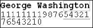
Figure 6-12
DECLARE @FullName VarChar(25)
SET @ FullName = ‘George Washington’
SELECT RIGHT(@FullName, 5)
Neither of these functions is particularly useful for consistently returning a meaningful part of this string. What if I wanted to return the first name or last name portions of the full name? This takes just a little more work. The LEFT() function may be the right method to use for extracting the first name if I can determine the position of the space in every name I might encounter. In this case, I can use the CHARINDEX() or PATINDEX() functions to locate the space and then use the LEFT() function to return only these characters. The first example here takes a procedural approach, breaking this process into steps:
DECLARE @FullName VarChar(25), @SpaceIndex TinyInt
SET @FullName = ‘George Washington’

-- Get index of the delimiting space:
SET @SpaceIndex = CHARINDEX(‘ ’, @FullName)

-- Return all characters to the left of the space:
SELECT LEFT(@FullName, @SpaceIndex - 1)
I don't want to include the space so it's necessary to subtract one from the @SpaceIndex value to include only the first name.
The SUBSTRING() Function
The SUBSTRING() function starts at a position and counts characters to the right, returning a substring of a specified length. Unlike the LEFT() function, you can tell it at what index position to begin counting. This allows you to extract a substring from anywhere within a character string. This function requires three arguments: the string to parse, the starting index, and the length of the substring to return. If you want to return all text to the end of the input string, you can use a length index larger than necessary. The SUBSTRING() function will return characters up to the last position of the string and will not pad the string with spaces.
The SUBSTRING() function can easily replace the LEFT() function by designating the left-most character of the string (1) as the starting index.
Continuing with the earlier example, I can set the starting position and length, returning a value from the middle of the name string. In this case, I'll start at position 4 and return a 6-character substring, as shown in Figure 6-13.
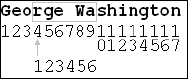
Figure 6-13
DECLARE @FullName VarChar(25)
SET @FullName = ‘George Washington’
SELECT SUBSTRING(@FullName, 4, 6)
Now, I'll put it all together and parse the first and last names from the full name in a way that will work for any full name string formatted as FirstName + space + LastName. Using the same logic as before, I'm going to nest the function calls to reduce the number of lines of script and get rid of the @SpaceIndex variable. Instead of the LEFT() function, I'll use SUBSTRING(). I've added a comment below the line that does all the work. Spaces are added to make room for the comment text:
DECLARE @FullName VarChar(25)
SET @FullName = ‘George Washington’
-- Return first name:
SELECT SUBSTRING(@FullName, 1,    CHARINDEX(‘ ’, @FullName) - 1)
--               ^String   ^Start ^Returns space index       ^Don't include space
Similar logic is used to extract the last name. I just have to change the start index argument to the position following the space. The space is at position seven and the last name begins at position eight. This means that the start index will always be one plus the CHARINDEX() result:
DECLARE @FullName VarChar(25)
SET @FullName = ‘George Washington’
SELECT SUBSTRING(@FullName, CHARINDEX(‘ ’, @FullName) + 1, LEN(@FullName))
The values passed into the SUBSTRING() function are the position of the space plus one as the start index. This will be the first letter of the last name. Because I won't always know the length of the name, I passed in the LEN() function for the length of the substring. The SUBSTRING() function will reach the end of the string when it reaches this position and simply include all characters after the space to the end of the string.
To set up an example, I'll create and populate a temporary table:
CREATE TABLE #MyNames (FullName    VarChar(50))
GO
INSERT INTO #MyNames (FullName) SELECT ‘Fred Flintstone’
INSERT INTO #MyNames (FullName) SELECT ‘Wilma Flintstone’
INSERT INTO #MyNames (FullName) SELECT ‘Barney Rubble’
INSERT INTO #MyNames (FullName) SELECT ‘Betty Rubble’
INSERT INTO #MyNames (FullName) SELECT ‘George Jetson’
INSERT INTO #MyNames (FullName) SELECT ‘Jane Jetson’
Now I'll execute a query using the function calls to parse the first name and last name values as one-line expressions. Note that references to the @FullName variable are replaced with the FullName column in the table:
SELECT
    SUBSTRING(FullName, 1, CHARINDEX(‘ ’, FullName) - 1) AS FirstName
  , SUBSTRING(FullName, CHARINDEX(‘ ’, FullName) + 1, LEN(FullName)) AS LastName
FROM #MyNames
The results shown in Figure 6-14 display two distinct columns as if the first and last names were stored separately.
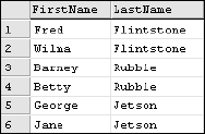
Figure 6-14
The LOWER() and UPPER() Functions
These functions are pretty easy to figure out. Each simply converts a character string to all lowercase or all uppercase characters. This is most useful when comparing user input or stored strings for comparison. String comparisons are typically case-insensitive, depending on settings chosen during SQL Server setup. Used along with other string manipulation functions, strings can be converted to use proper case for data storage and presentation. This example accounts for mixed-case last names, assuming the name contains a single space before the second capitalized substring. You could argue that some of these names normally wouldn't contain spaces, and I agree. This demonstration could easily be extended to include provisions for other mixed-case names (names beginning with Mc, hyphenated names, and so on).
DECLARE @LastName VarChar(25), @SpaceIndex TinyInt
SET @LastName = ‘mc donald’        -- Test value

-- Find space in name:
SET @SpaceIndex = CHARINDEX(‘ ’, @LastName)
IF @SpaceIndex > 0                       -- Space: Capitalize first & substring
    SELECT UPPER(LEFT(@LastName, 1))
  + LOWER(SUBSTRING(@LastName, 2, @SpaceIndex - 1))
  + UPPER(SUBSTRING(@LastName, @SpaceIndex + 1, 1))
  + LOWER(SUBSTRING(@LastName, @SpaceIndex + 2, LEN(@LastName))
ELSE                                     -- No space: Cap only first char.
    SELECT UPPER(LEFT(@LastName, 1))
  + LOWER(SUBSTRING(@LastName, 2, LEN(@LastName))
This script returns Mc Donald. I can also extend the example to deal with last names containing an apostrophe. The business rules in this case expect no space. If an apostrophe is found, the following character is to be capitalized. Note that to test an apostrophe in script, it must be entered twice (‘’) to indicate that this is a literal, rather than an encapsulating single quote. Last name values are stored with only an apostrophe.
DECLARE @LastName VarChar(25), @SpaceIndex TinyInt, @AposIndex TinyInt
SET @LastName = ‘o’ ‘malley’     -- Test value

-- Find space in name:
SET @SpaceIndex = CHARINDEX(‘ ’, @LastName)
-- Find literal ' in name:
SET @AposIndex = CHARINDEX(‘’‘’, @LastName)
IF @SpaceIndex > 0                       -- Space: Capitalize first & substring
    SELECT UPPER(LEFT(@LastName, 1))
  + LOWER(SUBSTRING(@LastName, 2, @SpaceIndex - 1))
  + UPPER(SUBSTRING(@LastName, @SpaceIndex + 1, 1))
  + LOWER(SUBSTRING(@LastName, @SpaceIndex + 2, LEN(@LastName))
ELSE IF @AposIndex > 0                   -- Apostrophe: Cap first & substring
    SELECT UPPER(LEFT(@LastName, 1))
  + LOWER(SUBSTRING(@LastName, 2, @AposIndex - 1))
  + UPPER(SUBSTRING(@LastName, @AposIndex + 1, 1))
  + LOWER(SUBSTRING(@LastName, @AposIndex + 2, LEN(LastName)))
ELSE                                     -- No space: Cap only first char.
    SELECT UPPER(LEFT(@LastName, 1))
  + LOWER(SUBSTRING(@LastName, 2, LEN(LastName)))
This script returns O'Malley. For this to be of use, I'll wrap it up into a user-defined function:
CREATE FUNCTION dbo.fn_FixLastName ( @LastName VarChar(25) )
RETURNS VarChar(25)
AS
BEGIN
  DECLARE  @SpaceIndex TinyInt
         , @AposIndex TinyInt
        , @ReturnName VarChar(25)
  -- Find space in name:
SET @SpaceIndex = CHARINDEX(‘ ’, @LastName)
  -- Find literal ' in name:
SET @AposIndex = CHARINDEXT(‘’‘’, @LastName)
IF @SpaceIndex > 0                        -- Space: Capitalize first & substring
         SET @ReturnName = UPPER(LEFT(@LastName, 1))
       + LOWER(SUBSTRING(@LastName, 2, @SpaceIndex - 1))
       + UPPER(SUBSTRING(@LastName, @SpaceIndex + 1, 1))
       + LOWER(SUBSTRING(@LastName, @SpaceIndex + 2, LEN(LastName)))
ELSE IF @AposIndex > 0                   -- Apostrophe: Cap first & substring
         SET @ReturnName = UPPER(LEFT(@LastName, 1))
       + LOWER(SUBSTRING(@LastName, 2, @AposIndex - 1))
       + UPPER(SUBSTRING(@LastName, @AposIndex + 1, 1))
       + LOWER(SUBSTRING(@LastName, @AposIndex + 2, LEN(LastName)))
ELSE                                     -- No space: Cap only first char.
         SET @ReturnName = UPPER(LEFT(@LastName, 1))
     + LOWER(SUBSTRING(@LastName, 2, LEN(LastName)))
RETURN @ReturnName
END
To test my function, I'll populate a temporary table with sample values so that I can query the names from this table:
CREATE TABLE #MyIrishFriends (FirstName VarChar(25), LastName VarChar(25) )

INSERT INTO #MyIrishFriends (FirstName, LastName) SELECT ‘James’, ‘O’‘grady’
INSERT INTO #MyIrishFriends (FirstName, LastName) SELECT ‘Nancy’, ‘o’‘brian’
INSERT INTO #MyIrishFriends (FirstName, LastName) SELECT ‘George’, ‘MC kee’
INSERT INTO #MyIrishFriends (FirstName, LastName) SELECT ‘Jonas’, ‘mc intosh’
INSERT INTO #MyIrishFriends (FirstName, LastName) SELECT ‘Florence’, ‘MC BRIDE’
The results as they are stored are shown in Figure 6-15.
SELECT FirstName, LastName FROM
#MyIrishFriends
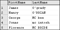
Figure 6-15
Using the custom function returns the results shown in Figure 6-16.
SELECT FirstName, dbo.fn_FixLastName(LastName) AS LastName
FROM #MyIrishFriends
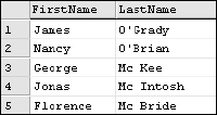
Figure 6-16
The LTRIM() and RTRIM() Functions
These two functions simply return a string with white space (spaces) trimmed from either the left or right side of significant characters:
DECLARE @Value1 Char(10), @Value2 Char(10)
SET @Value1 = ‘One’
SET @Value2 = ‘Two’
SELECT @Value1 + @Value2
SELECT CONVERT(VarChar(5), LEN(@Value1 + @Value2)) + ‘ characters long.’
SELECT RTRIM(@Value1) + RTRIM(@Value2)
SELECT CONVERT(VarChar(5), LEN(RTRIM(@Value1) + RTRIM(@Value2)))
       + ‘ characters long trimmed.’
The abbreviated results in text form follow:
-----------------
One Two
-------------------------
13 characters long.

-------------------
OneTwo
----------------------------
6 characters long trimmed.
The REPLACE() Function
The REPLACE() function can be used to replace all occurrences of one character or substring with another character or substring. This can be used as a global search and replace utility.
DECLARE @Phrase VarChar(1000)
SET @Phrase = ‘I aint gunna use poor grammar when commenting script and I aint
gunna complain about it.’
SELECT REPLACE(@Phrase, ‘aint’, ‘isn’‘t’)
As you can see, this was quite effective:
The REPLICATE() and SPACE() Functions
This is a very useful function when you need to fill a value with repeating characters. I'll use the same temporary table I created for the list of names in the SUBSTRING() example to pad each name value to 20 characters. I subtract the length of each value to pass the right value to the REPLICATE() function:
SELECT FullName + REPLICATE(‘*’, 20 - LEN(FullName))
FROM #MyNames
The result is a list of names padded with asterisk characters, each 20 characters in length:
Fred Flintstone*****
Wilma Flintstone****
Barney Rubble*******
Betty Rubble********
George Jetson*******
Jane Jetson*********
The SPACE() function does the same thing, only with spaces. It simply returns a string of space characters of a defined length.
The REVERSE() Function
This function reverses the characters in a string. This might be useful if you need to work with single-character values in a concatenated list.
I'm sure there's a practical application for this.
The STUFF() Function
This function allows you to replace a portion of a string with another string. It essentially will stuff one string into another string at a given position and for a specified length. This can be useful for string replacements where the source and target values aren't the same length. For example, I need to replace the price in this string, changing it from 99.95 to 109.95:
The price value begins at position 32 and is five characters in length. It really doesn't matter how long the substring is that I want to stuff into this position. I simply need to know how many characters need to be removed.
SELECT STUFF(‘Please submit your payment for 99.95 immediately.’, 32, 5, ‘109.95’)
The resulting string follows:
Please submit your payment for 109.95 immediately.
The QUOTENAME() Function
This function is used with SQL Server object names so they can be passed into an expression. It simply returns a string with square brackets around the input value. If the value contains reserved delimiting or encapsulating characters (such as quotation marks or brackets), modifications are made to the string so SQL Server perceives these characters as literals.
Image/Text Functions
The Text, nText, and Image data types define columns that can store up to 2 gigabytes of ANSI text, Unicode text, or binary data, respectively. SQL Server 2005 still has support for these data types, but Microsoft recommends the use of the new VarChar(max) and VarBinary(max) types in their place. These enhanced data types have the same capabilities and storage characteristics as their older counterparts, but they also support all of the string functions like standard character types. Older types may eventually be phased out of future SQL Server versions.
Two functions have specialized functionality specific to the Text, nText, and Image data types. Additionally, the PATINDEX() string function can be used to find a string of text within these columns and return an integer representing the character position of the first occurrence of the string.
Mathematical Functions
The functions listed in the following table are used to perform a variety of common and specialized mathematical operations and are useful in performing algebraic, trigonometric, statistical, approximating, and financial operations.
Metadata Functions
These are utility functions that return information about the SQL Server configuration details and details about the server and database settings. This includes a range of general and special-purpose property-related functions that will return the state of various object properties. These functions wrap queries from the system tables in the Master database and a user database. It's recommended that you use these and other system functions rather than creating queries against the system tables yourself, in case schema changes are made in future versions of SQL Server. Some of the information listed in the following table can also be obtained using the INFORMATION_SCHEMA views.
Ranking Functions
These are new functions in SQL Server 2005 used to enumerate sorted and top-valued result sets using a specified order, independent from the order of the result set.
The ROW_NUMBER() Function
The ROW_NUMBER() function returns an integer with a running incremental value based on an ORDER BY clause passed to this function. If the ROW_NUMBER's ORDER BY matches the order of the result set, the values will be incremental and in ascending order. If the ROW_NUMBER's ORDER BY clause is different than the order of the results, these values will not be listed in order but will represent the order of the ROW_NUMBER function's ORDER BY clause.
SELECT
    ProductCategorylD
  , Name
  , ROW_NUMBER() Over (ORDER BY Name) As RowNum
FROM ProductCategory
ORDER BY Name
With the ORDER BY clause on the ROW_NUMBER() call matching the order of the query, these values are listed in order (see Figure 6-17).
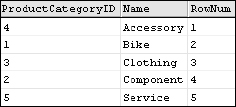
Figure 6-17
However, when using a different ORDER BY clause in the function call, these values are not ordered.
SELECT
    ProductCategoryID
  , Name
  , ROW_NUMBER() Over (ORDER BY Name) As RowNum
FROM ProductCategory
ORDER BY ProductCategoryID
This provides an effective means to tell how the result would have been sorted using the other ORDER BY clause, as shown in Figure 6-18.
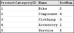
Figure 6-18
The RANK() and DENSE_RANK() Functions
Both of these functions are similar to the ROW_NUMBER() function in that they return a value based on an ORDER BY clause, but these values may not always be unique. Ranking values are repeated for duplicate results from the provided ORDER BY clause, and uniqueness is only based on unique values in the ORDER BY list. Each of these functions takes a different approach to handling these duplicate values. The RANK() function preserves the ordinal position of the row in the list. For each duplicate value, it skips the subsequent value so that the next non-duplicate value remains in its rightful position.
SELECT
    ProductCategorylD
  , Name
  , RANK() Over (ORDER BY Name) As Rank
FROM ProductCategory
ORDER BY Name
Note in the result set shown in Figure 6-19 that the values are repeated for duplicated name values and the skipped values following each tie. For example, both rows for employees named Andrew are ranked number 8, and the following row, Andy, is ranked number 10.
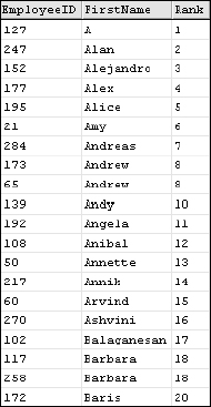
Figure 6-19
The DENSE_RANK() function works exactly the same way, but it doesn't skip numbers after each tie. This way, no values are skipped, but the ordinal ranking position is lost whenever there are ties.
SELECT
    ProductCategoryID
  , Name
  , DENSE_RANK() Over (ORDER BY Name) As Rank
FROM ProductCategory
ORDER BY Name
The result shown in Figure 6-20 repeats ranked values but doesn't skip any numbers in this column.
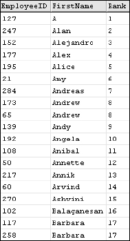
Figure 6-20
The NTILE(n) Function
This function also ranks results, returning an integer ranking value. However, rather than enumerating the results into uniquely ranked order, it divides the result into a finite number of ranked groups. For example, if a table has 10,000 rows and the NTILE() function is called with an argument value of 1000, as NTILE(1000), the result would be divided into 1000 groups of 10, with each group being assigned the same ranking value. The NTILE() function also supports the OVER (ORDER BY…) syntax like the other ranking functions discussed in this section.
Security Functions
The security-related functions return role membership and privilege information for SQL Server users. This category also includes a set of functions to manage events and traces, as described in the following table.
System Functions and Variables
This section discusses utility functions used to perform a variety of tasks. These include value comparisons and value type testing. This category is also a catch-all for other functionality.
Some examples related to a few of the functions listed in the preceding table follow.
The COALESCE() Function
The COALESCE() function can be very useful, saving quite a lot of IF or CASE decision logic. The following example populates a table of products, showing up to three prices each:
CREATE TABLE #ProductPrices (ProductName VarChar(25), SuperSalePrice Money NULL,
SalePrice Money NULL, ListPrice Money NULL)
GO
INSERT INTO #ProductPrices VALUES(‘Standard Widget’, NULL, NULL, 15.95)
INSERT INTO #ProductPrices VALUES(‘Economy Widget’, NULL, 9.95, 12.95)
INSERT INTO #ProductPrices VALUES(‘Deluxe Widget’, 19.95, 20.95, 22.95)
INSERT INTO #ProductPrices VALUES(‘Super Deluxe Widget’, 29.45, 32.45, 38.95)
INSERT INTO #ProductPrices VALUES(‘Executive Widget’, NULL, 45.95, 54.95)
GO
All products have a list price, some have a sale price, and others may have a super sale price. The current price of a product is going to be the lowest existing price, or the first non-null value when reading each of the price columns as they are listed:
SELECT ProductName, COALESCE(SuperSalePrice, SalePrice, ListPrice) AS CurrentPrice
FROM #ProductPrices
This method is far more elegant than using multiple lines of branching and decision logic, and the result is equally simple, as illustrated in Figure 6-21.
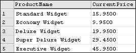
Figure 6-21
The DATALENGTH() Function
The DATALENGTH() function returns the number of bytes used to manage a value. This can be used to reveal some interesting differences between data types. It's probably no surprise that when a VarChar type is passed to both the DATALENGTH() and LEN() functions, they return the same value:
DECLARE @Value VarChar(20)
SET @Value = ‘abc’

SELECT DATALENGTH(@Value)
SELECT LEN(@Value)
These statements both return 3 because the VarChar type uses three single-byte characters to store the three-character value. However, if an nVarChar type is used, it takes twice as many bytes to manage a value of the same length:
DECLARE @Value nVarChar(20)
SET @Value = ‘abc’

SELECT DATALENGTH(@Value)
SELECT LEN(@Value)
The DATALENGTH() function returns 6 because 2 bytes are used to store each character using a Unicode character set. The LEN() function returns 3 because this function returns the number of characters, not the number of bytes. Here's an interesting test. How many bytes does it take to store an integer variable set to the value 2? How about an integer a variable set to 2 billion? Let's find out:
DECLARE @Value1 Int, @Value2 Int
SET @Value1 = 2
SET @Value2 = 2000000000

SELECT DATALENGTH(@Value1)
SELECT LEN(@Value1)

SELECT DATALENGTH(@Value2)
SELECT LEN(@Value2)
The DATALENGTH() function returns 4 in both cases because the Int type always uses 4 bytes, regardless of the value. The LEN() function essentially treats the integer value as if it were converted to a character type, returning the number of digits, in this case, 1 and 10, respectively.
The following global system variables all return an Int type. These may be useful in stored procedures and other programming objects to implement custom business logic.
| Variable | Description |
| @@ERROR | The last error number for the current session. |
| @@IDENTITY | The last identity value generated in the current session. |
| @@ROWCOUNT | The row count for the last execution in the current session that returned a result set. |
| @@TRANCOUNT | The number of active transactions in the current session. This would result from multiple, nested BEGIN TRANSACTION statements before executing corresponding COMMIT TRANSACTION or ABORT TRANSACTION statements. |
System Statistical Functions and Variables
The following table describes administrative utilities used to discover database system usage and environment information.
| Variable | Description |
| @@CONNECTIONS | The number of open connections. |
| @@CPU_BUSY | The number of milliseconds that SQL Server has been working since the service was last started. |
| @@IDLE | The number of milliseconds that SQL Server has been idle since the service was last started. |
| @@IO_BUSY | The number of milliseconds that SQL Server has been processing I/O since the service was last started. |
| @@PACK_RECEIVED | The number of network packets that SQL Server has received since the service was last started. |
| @@PACK_SENT | The number of network packets that SQL Server has sent since the service was last started. |
| @@PACKET_ERRORS | The number of network packet errors that SQL Server has received since the service was last started. |
| @@TIMETICKS | The number of microseconds per tick. |
| @@TOTAL_ERRORS | The number of disk I/O errors that SQL Server has received since the service was last started. |
| @@TOTAL_READ | The number of physical disk reads since the SQL Server service was last started. |
| @@TOTAL_WRITE | The number of physical disk writes since the SQL Server service was last started. |
Summary
Functions do the heavy lifting of your business logic and can be used to apply programming functionality to queries. Several useful and powerful functions are standard features of Transact-SQL. You learned that SQL functions, like functions in procedural and object-oriented programming languages, encapsulate programming features into a simple and reusable package. This takes a lot of the work out of the query designer's hands. You know that Transact-SQL is a task-oriented language rather than a procedural language. Although functions give you the option to tread the procedural line, building fairly complex logic into queries, the strength of the language is in allowing the designer to state his intentions rather than the exact steps and methods that must be used to perform a task. Used correctly, functions allow you to do just that.
In Transact-SQL, arguments are used to pass values into a function and most functions return a scalar, or single-value, result. Functions are categorized as either deterministic or nondeterministic. A deterministic function will always return the same value when called with the same argument values. Nondeterministic functions depend on other resources to determine the return value; therefore SQL Server must execute the function explicitly. For this reason, there are some restrictions on the use of nondeterministic functions in custom SQL programming objects.
SQL functions perform a wide variety of important tasks including mathematical operations, comparisons, date parsing and manipulation, and advanced string manipulation. Several categories of specialized functions are introduced along with their related topics in following chapters. A complete function syntax reference is also provided in Appendix B.
Exercises
Exercise 1
Write a query to return the average weight of all touring bikes sold by Adventure Works Cycles that list for over $2,500. Use the ProductSubCategory table to determine how you should filter these products.
Exercise 2
Designate a variable called @ProCount to hold the number of product records on record. Execute a query to return this value and assign it to the variable. Use the variable in an expression to return the value in the phrase “There are X products on record.”
Exercise 3
Calculate the square root of the absolute value of the cosine of PI.
Exercise 4
How many days has it been since this book was first published on September 26, 2005? Calculate the answer using Transact-SQL functions.
Exercise 5
Using the Individual table, return the FirstName, LastName, and the three-letter initials of all individuals who have a middle name.