
5.4.3 FOREST TERRAIN
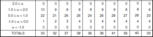
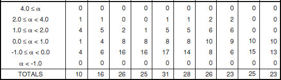
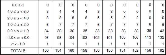
Much natural terrain is forested. The characteristics of land clutter from forested terrain are very different than from open terrain. Section 5.4.3 specifies the characteristics of forest land clutter based on 8,611 measured clutter histograms from 466 forest clutter patches. These measurements break down in two regimes of relief, high (terrain slopes > 2°) and low (terrain slopes < 2°), and in multiple depression angle regimes as shown in Table 5.24. These forest clutter measurements come from 27 different sites.
TABLE 5.24
Numbers of Terrain Patches and Measured Clutter Histograms for Forest, by Relief and Depression Anglea,b,c
aA single (primary) classifier only is sufficient to describe these patches.
bA terrain patch is a land surface macroregion usually several kms on a side (median patch area = 12.62 km2).
cA measured clutter histogram contains all of the temporal (pulse by pulse) and spatial (resolution cell by resolution cell) clutter samples obtained in a given measurement of a terrain patch. A terrain patch was usually measured many times (nominally 20) as RF frequency (5), polarization (2), and range resolution (2) were varied over the Phase One radar parameter matrix.
Because forest is much less supportive of multipath than is open terrain, particularly at high illumination angles, many of these forest measurements are much more measurements of relatively pure intrinsic σ° and are much less contaminated by dispersive propagation influences than are measurements in open terrain. To the extent that this is true, fewer measurements can establish trends in forest terrain than in farmland terrain. Nevertheless, the Phase One forest clutter measurements constitute 29% of all Phase One measurements in pure terrain. Thus, after farmland at 35%, forest stands as far and away the second most highly sampled terrain type among the eight pure terrain types of Chapter 5.
Classification of forest clutter patches was in three separate categories, viz., deciduous, coniferous, and mixed (see Table 2.1). However, the clutter measurements showed no significant variation among these classes. The results presented here are inclusive of all three classes.
Little seasonal variation was observed in the Phase One clutter measurements from forested terrain. One forested wilderness site—Brazeau, Alberta—was visited twice by the Phase One equipment, once in summer and once in winter. Typically, mean clutter strengths at
Brazeau between summer and winter seasons differed by only 1 or 2 dB with the summer measurements usually (but not always) being stronger (see Section 3.4.1.3.3 and Figure 3.24). The results presented in Section 5.4.3 are inclusive of all Phase One forest measurements independent of the season in which the measurement was made. As was provided for agricultural terrain, some interpretative discussion involving individual patch measurements continues to be provided concerning the uncertain outliers that occur in the following results for forest terrain.
It is interesting to compare the high- and low-relief forest mean clutter strength data to follow with the site-specific repeat-sector forest mean clutter strength characteristics from Blue Knob and Wachusett Mountain shown in Figures 3.3 and 3.4, respectively, in Chapter 3.
5.4.3.1 HIGH-RELIEF FOREST
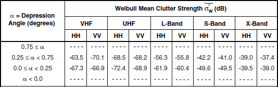
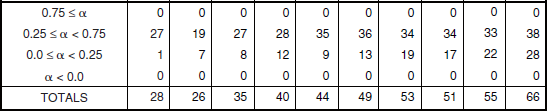
Trends in ![]() . Table 5.25 presents mean clutter strength
. Table 5.25 presents mean clutter strength ![]() for high-relief forest by frequency band, polarization, and depression angle and includes the number of measurements upon which each value of
for high-relief forest by frequency band, polarization, and depression angle and includes the number of measurements upon which each value of ![]() is based. A relatively large amount of Phase One measurement data exists for high-relief forest—more than 10 times that which exists for high-relief farmland, for example (compare Tables 5.16 and 5.24), and approximately the same as exists for low-relief forest (see Table 5.24). Much of these data exist in the lower, 0° to 1° and 0° to −1°, depression angle regimes. At higher depression angles the amount of available data falls off rapidly. In particular, Table 5.25 shows that no data exist above 2° at X-band, above 4° at S-band, and above 6° at L-band. This lack of data at high angles results from the fact that the Phase One antenna elevation beam is always directed horizontally and is of decreasing beamwidth with increasing frequency, e.g., 10° at L-band (i.e., the half-power point is 5° above the horizontal), 4° at S-band, and 3° at X-band (see Table 3.A.2). Of course, all σ°F4 measurement data upon which Chapter 5 is based are corrected for antenna gain depending exactly where on the vertical pattern the particular measurement is made. Data requiring a two-way correction of more than about 10 dB are not utilized. Although the Phase One equipment is constrained to relatively narrow vertical beamwidths in the higher bands, with corresponding lack of measurement data at higher depression angles, the Phase Zero equipment had a much broader vertical beamwidth (viz., 23°), and as a result the Phase Zero database does provide land clutter results—albeit at X-band only—to higher depression angles (e.g., 8°, see Chapter 2).
is based. A relatively large amount of Phase One measurement data exists for high-relief forest—more than 10 times that which exists for high-relief farmland, for example (compare Tables 5.16 and 5.24), and approximately the same as exists for low-relief forest (see Table 5.24). Much of these data exist in the lower, 0° to 1° and 0° to −1°, depression angle regimes. At higher depression angles the amount of available data falls off rapidly. In particular, Table 5.25 shows that no data exist above 2° at X-band, above 4° at S-band, and above 6° at L-band. This lack of data at high angles results from the fact that the Phase One antenna elevation beam is always directed horizontally and is of decreasing beamwidth with increasing frequency, e.g., 10° at L-band (i.e., the half-power point is 5° above the horizontal), 4° at S-band, and 3° at X-band (see Table 3.A.2). Of course, all σ°F4 measurement data upon which Chapter 5 is based are corrected for antenna gain depending exactly where on the vertical pattern the particular measurement is made. Data requiring a two-way correction of more than about 10 dB are not utilized. Although the Phase One equipment is constrained to relatively narrow vertical beamwidths in the higher bands, with corresponding lack of measurement data at higher depression angles, the Phase Zero equipment had a much broader vertical beamwidth (viz., 23°), and as a result the Phase Zero database does provide land clutter results—albeit at X-band only—to higher depression angles (e.g., 8°, see Chapter 2).
TABLE 5.25
Mean Clutter Strength ![]() and Number of Measurements for High-Relief Forest, by Frequency Band, Polarization, and Depression Anglea
and Number of Measurements for High-Relief Forest, by Frequency Band, Polarization, and Depression Anglea
aTable 5.24 defines the population of terrain patches upon which these data are based.
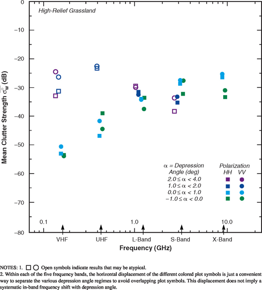
The high-relief forest ![]() data of Table 5.25 are plotted in Figure 5.24. The main characteristics of the data in Figure 5.24 are similar to those of high-relief general mixed rural terrain shown in Figure 5.8 and discussed in Section 5.3. In particular, like the high-relief general mixed rural
data of Table 5.25 are plotted in Figure 5.24. The main characteristics of the data in Figure 5.24 are similar to those of high-relief general mixed rural terrain shown in Figure 5.8 and discussed in Section 5.3. In particular, like the high-relief general mixed rural ![]() data, the high-relief forest
data, the high-relief forest ![]() data show significantly decreasing strength with increasing frequency, VHF to S-band, with a subsequent small increase, S-band to X-band; and also, like the high-relief general mixed rural data, the high-relief forest data show the v-shapes within frequency bands indicating strong effects from depression angle.
data show significantly decreasing strength with increasing frequency, VHF to S-band, with a subsequent small increase, S-band to X-band; and also, like the high-relief general mixed rural data, the high-relief forest data show the v-shapes within frequency bands indicating strong effects from depression angle.
Next, consider the effects of depression angle on the high-relief forest ![]() data in Figure 5.24 more closely. Focus first on the cyan, 0° to 1° results. In each frequency band, there is a general trend of increasing
data in Figure 5.24 more closely. Focus first on the cyan, 0° to 1° results. In each frequency band, there is a general trend of increasing ![]() with increasing positive depression angle, from cyan (0° to 1°) to dark blue (1° to 2°) to purple (2° to 4°) to magenta (4° to 6°) to red (> 6°); and also a general trend of increasing
with increasing positive depression angle, from cyan (0° to 1°) to dark blue (1° to 2°) to purple (2° to 4°) to magenta (4° to 6°) to red (> 6°); and also a general trend of increasing ![]() with increasing negative depression angle, from cyan (0° to 1°) to dark green (0° to −1°) to intermediate green (< −1°). These trends of increasing
with increasing negative depression angle, from cyan (0° to 1°) to dark green (0° to −1°) to intermediate green (< −1°). These trends of increasing ![]() with increasing positive and negative depression angle in high-relief forest terrain, although very significant, are not quite as smooth or as nearly monotonic as in high-relief general mixed rural terrain (notably, there is a reversal in trend between the dark blue, 1° to 2°, high-relief forest
with increasing positive and negative depression angle in high-relief forest terrain, although very significant, are not quite as smooth or as nearly monotonic as in high-relief general mixed rural terrain (notably, there is a reversal in trend between the dark blue, 1° to 2°, high-relief forest ![]() results and the purple, 2° to 4°, high-relief forest
results and the purple, 2° to 4°, high-relief forest ![]() results at VHF and UHF, and to a lesser degree in the horizontal polarization results at L-band; the weak, purple, 2° to 4° results at S-band plotted as open plot symbols will be discussed presently). This may be due to the fact that the amount of Phase One clutter measurement data available for high-relief forest, although large, is still only about 30% of the amount of data available for high-relief general mixed rural terrain (e.g., there are only 10 patches contributing to the 2° to 4° regime; see Table 5.24).
results at VHF and UHF, and to a lesser degree in the horizontal polarization results at L-band; the weak, purple, 2° to 4° results at S-band plotted as open plot symbols will be discussed presently). This may be due to the fact that the amount of Phase One clutter measurement data available for high-relief forest, although large, is still only about 30% of the amount of data available for high-relief general mixed rural terrain (e.g., there are only 10 patches contributing to the 2° to 4° regime; see Table 5.24).
The v-shapes of the set of colored plot symbols in each frequency band for the high-relief forest ![]() data in Figure 5.24 have less vertical extent (disregarding the open plot symbols) than the corresponding v-shapes for the high-relief general mixed rural data of Figure 5.8. Both Figure 5.24 and Figure 5.8 provide
data in Figure 5.24 have less vertical extent (disregarding the open plot symbols) than the corresponding v-shapes for the high-relief general mixed rural data of Figure 5.8. Both Figure 5.24 and Figure 5.8 provide ![]() results in the same ranges at high positive depression angles. The differences accounting for less in-band vertical extent in Figure 5.24 are in the low depression angle (i.e., cyan) results. In each frequency band, the cyan, 0 to 1°,
results in the same ranges at high positive depression angles. The differences accounting for less in-band vertical extent in Figure 5.24 are in the low depression angle (i.e., cyan) results. In each frequency band, the cyan, 0 to 1°, ![]() results for high-relief forest are greater than for high-relief general mixed rural terrain, by 6 or 7 dB at VHF, by 4 or 5 dB at UHF, by 2 or 3 dB at L-band, by about 2 dB at S-band, and by 1 or 2 dB at X-band. The fact that high-relief general mixed rural terrain is partially open reduces its clutter strength compared to high-relief forested terrain at low depression angle but not at high depression angle. At low angles more shadowing occurs of the open areas between forested areas in general mixed rural terrain than occurs in forested terrain, which is more uniformly illuminated; whereas, at high angles, relatively complete illumination occurs in mixed as well as forested terrain.
results for high-relief forest are greater than for high-relief general mixed rural terrain, by 6 or 7 dB at VHF, by 4 or 5 dB at UHF, by 2 or 3 dB at L-band, by about 2 dB at S-band, and by 1 or 2 dB at X-band. The fact that high-relief general mixed rural terrain is partially open reduces its clutter strength compared to high-relief forested terrain at low depression angle but not at high depression angle. At low angles more shadowing occurs of the open areas between forested areas in general mixed rural terrain than occurs in forested terrain, which is more uniformly illuminated; whereas, at high angles, relatively complete illumination occurs in mixed as well as forested terrain.
In the high-relief forest ![]() data of Table 5.25 and Figure 5.24,
data of Table 5.25 and Figure 5.24, ![]() is generally greater than
is generally greater than ![]() by several dB at VHF and UHF, and by a lesser amount at S-band. This polarization bias is less evident at L-band and X-band.
by several dB at VHF and UHF, and by a lesser amount at S-band. This polarization bias is less evident at L-band and X-band.
Radars are frequently situated in rural terrain that is often either forest or farmland. How important is the difference in land cover between forest and farmland in affecting the clutter amplitude statistics in the radar? Comparison between Figures 5.18 and 5.24 (and Tables 5.17 and 5.25) indicates that in high-relief terrain ![]() is significantly stronger in forest than in farmland. In broad measure, the amount of the difference by frequency band is: at VHF, 15 dB; at UHF, 10 dB; and at L-, S-, and X-bands, 3 to 6 dB.
is significantly stronger in forest than in farmland. In broad measure, the amount of the difference by frequency band is: at VHF, 15 dB; at UHF, 10 dB; and at L-, S-, and X-bands, 3 to 6 dB.
Uncertain Outliers. Now consider the uncertain outliers in ![]() in high-relief forest terrain which are plotted as open plot symbols in Figure 5.24. First consider the light green, <–1° results. These light green results are very strong at VHF, UHF, and L-band. Table 5.25 shows that these light green results are based on relatively few measurements. Table 5.24 shows that these few measurements come from just two patches. Both patches are of steep forested terrain in the region where the prairie transitions into the Rocky Mountains. Both patches were measured at relatively long range from Alberta prairie sites. Specifically, these patches are patch 105 at the Phase One measurement site of Strathcona, and patch 50 at the Phase One measurement site of Pakowki Lake. Patch 105 is moderately steep, pure forest terrain measured at 48-km range and at a 3000 ft higher elevation than the Strathcona site location. Patch 50 is steep, pure forest terrain measured at 65-km range and at a 3,300 ft higher elevation than the Pakowki Lake site location. The depression angle to patch 105 is −1.2°; to patch 50 is −1.1°.
in high-relief forest terrain which are plotted as open plot symbols in Figure 5.24. First consider the light green, <–1° results. These light green results are very strong at VHF, UHF, and L-band. Table 5.25 shows that these light green results are based on relatively few measurements. Table 5.24 shows that these few measurements come from just two patches. Both patches are of steep forested terrain in the region where the prairie transitions into the Rocky Mountains. Both patches were measured at relatively long range from Alberta prairie sites. Specifically, these patches are patch 105 at the Phase One measurement site of Strathcona, and patch 50 at the Phase One measurement site of Pakowki Lake. Patch 105 is moderately steep, pure forest terrain measured at 48-km range and at a 3000 ft higher elevation than the Strathcona site location. Patch 50 is steep, pure forest terrain measured at 65-km range and at a 3,300 ft higher elevation than the Pakowki Lake site location. The depression angle to patch 105 is −1.2°; to patch 50 is −1.1°.
The clutter from these two patches is very strong at VHF, UHF, and L-band (open, light green, plot symbols; Figure 5.24). The terrain from which this strong clutter arises is steep enough that it might be thought of as being mountainous. However, the term “mountains” is relatively vague and imprecise in terrain classification. In Chapter 5, mountain clutter data are constrained to come from two canonical Rocky Mountain clutter sites in which steep, barren (or snow-covered) mountain peaks and rock faces are visually and unambiguously present at close range—see Section 5.4.8. Other steep terrain from which Phase One measurements were made, for example, in the American Intermontane desert regions in the west or in the Appalachian Mountains in the east, is simply classified as high-relief, of whatever land cover type is appropriate. Thus it is apparent that considerable overlap exists between the classification categories of “high-relief” and “mountains” in Chapter 5—“mountains” being a relatively arbitrary subset of the general category of “high-relief.” A further subcategory of long-range mountains is employed in Section 5.4.8.1, within which the two patches under present discussion would fall in terms of their range and depression angle values if it were not that their land covers were pure forest.
The two patches in question, patch 105 at Strathcona and patch 50 at Pakowki Lake, properly meet the criteria for pure forest terrain (i.e., no barren peaks) of very high-relief. In fact, the clutter strengths from these two patches at VHF (vertical polarization only), UHF, and L-band are somewhat stronger than the corresponding general ![]() levels for mountains specified in Section 5.4.8 and much stronger in these bands than the corresponding levels for long-range mountains specified in Section 5.4.8.1. The results for these two patches are shown as open plot symbols in Figure 5.24 because, being from only two patches, these results cannot be considered general. No measurements of these two patches are available at S-band. At X-band, of these two patches only measurements of the Pakowki Lake patch are available; although not overly strong at X-band, these light green X-band results are still shown as open plot symbols in Figure 5.24 because of the little data involved (i.e., only one measurement at each polarization).
levels for mountains specified in Section 5.4.8 and much stronger in these bands than the corresponding levels for long-range mountains specified in Section 5.4.8.1. The results for these two patches are shown as open plot symbols in Figure 5.24 because, being from only two patches, these results cannot be considered general. No measurements of these two patches are available at S-band. At X-band, of these two patches only measurements of the Pakowki Lake patch are available; although not overly strong at X-band, these light green X-band results are still shown as open plot symbols in Figure 5.24 because of the little data involved (i.e., only one measurement at each polarization).
At S-band in Figure 5.24, the purple, 2° to 4° results are weaker and out-of-line with the other S-band results. Table 5.25 shows that none of the 2° to 4° results are based on a very large number of measurements, and that the S-band results in particular are based upon about one-half the number of measurements as the VHF, UHF, and L-band results.
Therefore, the S-band results are plotted as open plot symbols to indicate that they should be used with caution. Nevertheless, the purple, 2° to 4° high-relief forest ![]() data provide another indication of an S-band dip at high depression angle, similar, for example, to that previously discussed for general rural terrain.
data provide another indication of an S-band dip at high depression angle, similar, for example, to that previously discussed for general rural terrain.
VHF Polarization Bias. In the intermediate green, <–1°, VHF ![]() results in Figure 5.24 and Table 5.25,
results in Figure 5.24 and Table 5.25, ![]() by 9 dB. This large polarization bias at VHF disappears at UHF and L-band. This VHF polarization bias exists throughout the set of nine measurements from the two patches, patch 50 at Pakowki Lake and patch 105 at Strathcona, upon which these results are based; that is, this polarization bias is not a peculiarity of data reduction but exists in each corresponding pair of measurements from these two patches. Now consider the dark green, 0° to −1°, VHF
by 9 dB. This large polarization bias at VHF disappears at UHF and L-band. This VHF polarization bias exists throughout the set of nine measurements from the two patches, patch 50 at Pakowki Lake and patch 105 at Strathcona, upon which these results are based; that is, this polarization bias is not a peculiarity of data reduction but exists in each corresponding pair of measurements from these two patches. Now consider the dark green, 0° to −1°, VHF ![]() results in Figure 5.24 and Table 5.25. These dark green VHF results also exhibit a large polarization bias,
results in Figure 5.24 and Table 5.25. These dark green VHF results also exhibit a large polarization bias, ![]() by 7 dB. However, the dark green, 0° to −1° VHF results are based on many measurements from a large number of patches.
by 7 dB. However, the dark green, 0° to −1° VHF results are based on many measurements from a large number of patches.
A similar strong polarization bias, ![]() at VHF in high-relief terrain, is discussed in Section 3.4.1.2. This previous discussion is based on Phase One repeat sector measurements at the two Phase One mountain sites in Alberta, Plateau Mountain and Waterton. In the repeat sector measurements at these two mountain sites,
at VHF in high-relief terrain, is discussed in Section 3.4.1.2. This previous discussion is based on Phase One repeat sector measurements at the two Phase One mountain sites in Alberta, Plateau Mountain and Waterton. In the repeat sector measurements at these two mountain sites, ![]() by 7 to 8 dB. This bias is very similar to that exhibited in the light green (< −1°) and dark green (0° to −1°) high-relief forest data of Figure 5.24.
by 7 to 8 dB. This bias is very similar to that exhibited in the light green (< −1°) and dark green (0° to −1°) high-relief forest data of Figure 5.24.
In Chapter 5, which is based on the spatially comprehensive Phase One 360° survey data, similar strong VHF polarization biases occur for other high-relief forested terrain types. Usually the bias is much more pronounced in the dark green, 0° to −1° depression angle regime than at other depression angles, although similar but smaller biases of 2 or 3 dB, ![]() , frequently exist in the other depression angle regimes also. Thus, at VHF in the dark green, 0° to −1° results,
, frequently exist in the other depression angle regimes also. Thus, at VHF in the dark green, 0° to −1° results, ![]() : by 4.8 dB in high-relief general mixed rural terrain, by 7.0 dB in high-relief forest, by 9.8 dB in high-relief shrubland, by 9.6 dB in mountains, by 6.2 dB in high-relief mixed forest/open terrain, and by 6.8 dB in high-relief mixed open/forest terrain (forest/open and open/forest results are not included in this book). Thus, a large polarization bias at VHF occurs generally in high-relief forested terrain, predominantly in the 0° to −1° depression angle regime.
: by 4.8 dB in high-relief general mixed rural terrain, by 7.0 dB in high-relief forest, by 9.8 dB in high-relief shrubland, by 9.6 dB in mountains, by 6.2 dB in high-relief mixed forest/open terrain, and by 6.8 dB in high-relief mixed open/forest terrain (forest/open and open/forest results are not included in this book). Thus, a large polarization bias at VHF occurs generally in high-relief forested terrain, predominantly in the 0° to −1° depression angle regime.
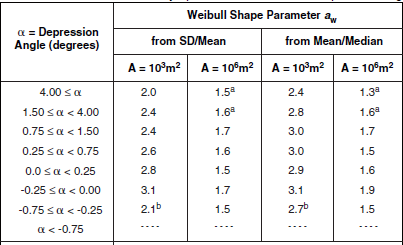
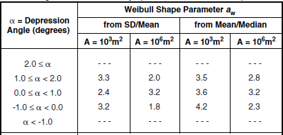
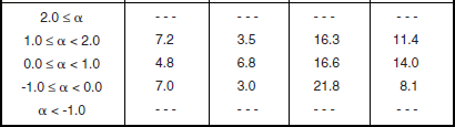
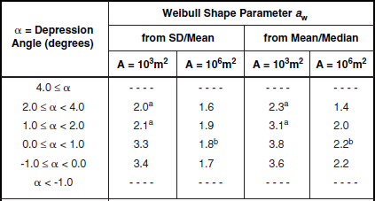
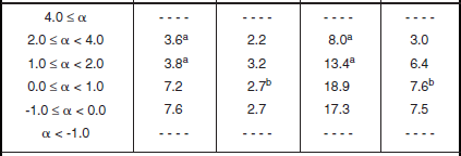
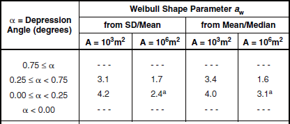
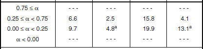
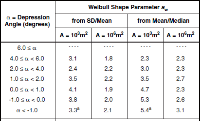
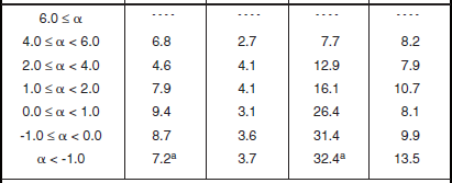
Shape Parameter aw. Table 5.26 presents the Weibull shape parameter aw and ratios of standard deviation-to-mean and mean-to-median for clutter amplitude distributions in high-relief forest terrain by depression angle and radar spatial resolution. The statistical populations underlying the data of Table 5.26 are shown in Table 5.24. Table 5.26 shows that the spread in spatial clutter amplitude distributions in high-relief forest terrain is much lower than in open terrain. Thus, for example, high-relief forest clutter is distinguished from high-relief farmland clutter, not just in terms of mean clutter strength as discussed previously in Section 5.4.3.1, but also in terms of spread—mean strengths are higher (i.e., more severe) and spreads are lower (i.e., less severe) in forest than in farmland. Spreads are lower in forest than in farmland because forest is a much more homogeneous scattering medium than farmland.
TABLE 5.26
Shape Parameter aw and Ratios of Standard Deviation-to-Mean (SD/Mean) and Mean-to-Median for High-Relief Forest, by Spatial Resolution A and Depression Angle*
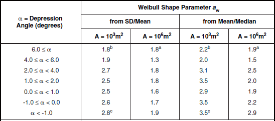
aFootnoted values apply at A = 105 m2, not 106 m2.
bFootnoted values apply at A = 104 m2, not 103 m2.
cFootnoted values apply at A = 105 m2, not 103 m2.
*Table 5.24 defines the population of terrain patches and measurements upon which these data are based.
Although the spreads shown in Table 5.26 for high-relief forest are lower than for most other terrain types, they still indicate a statistical process with considerable more spread than a Rayleigh (i.e., exponential power) process. In Rayleigh statistics, the Weibull shape parameter aw equals unity, and the ratios of mean-to-median and standard deviation-to-mean are 1.6 and 0 dB, respectively. Even at A = 106 m2 in Table 5.26, where spreads are least, they still generally remain much greater than Rayleigh. Although at the higher illumination angles of airborne radar, land clutter is in large measure a Rayleigh process, the data of Table 5.26 indicate that, for surface radar, land clutter is not a Rayleigh process, even at relatively high angles (for surface radar) in homogeneous forest terrain and with large resolution cells. Modeling of land clutter in surface radars as a Rayleigh process results in overestimates of radar detection performance. The actual clutter distributions that exist, skewed significantly more highly than Rayleigh even in forest terrain, cause, for example, higher numbers of false alarms for a given detection probability.
The main trend of parametric variation of aw in Table 5.26 is with radar spatial resolution. In almost every case, aw is greater at 103 m2 resolution than at 106 m2 resolution. However, this trend of decreasing aw with decreasing resolution is weaker in high-relief forest than in high-relief farmland. Values of aw at A = 103 m2 are generally considerably less in high-relief forest than in high-relief farmland; values of aw at A = 106 m2 are much closer for the two terrain types. There is only a secondary trend, relatively weak and erratic, whereby aw decreases with increasing depression angle in Table 5.26, although the numbers of measurements are quite low at the higher depression angles.
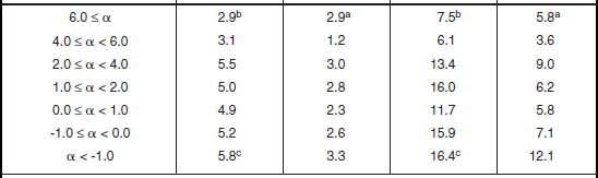
Each pair of aw numbers in Table 5.26 comes from a scatter plot of spread vs spatial resolution. The standard deviation-to-mean scatter plot for the 2° to 4° depression angle regime in Table 5.26 is shown in Figure 5.25. The data in Figure 5.25 show a significant trend of decreasing spread with decreasing resolution (i.e., increasing A), although the trend is by no means as strong as that shown previously for high-relief farmland, 1° to 2°, in Figure 5.19. Comparison of Figures 5.25 and 5.19 provides graphic indication of the much lower spreads that exist in land clutter spatial amplitude distributions for forest terrain compared to farmland.
5.4.3.2 LOW-RELIEF FOREST
visibility and Shadow. Low-relief forest is a simple scattering surface compared with other terrain types. There are several contributing aspects to this simplicity. First, low-relief forest is not dominated by large cultural discrete scattering sources spatially distributed in deterministic patterns as is farmland, but is much more a natural homogeneous random scattering medium. Second, low-relief forest is a diffusely scattering medium and does not, to any significant degree, support forward multipath reflections that cause high complexity in illumination and resulting clutter strength in open terrain. Third, low-relief forest, being of low-relief, is not dominated by particular large-scale terrain features, but has only minor undulations, inclinations, and waviness in the surface. Because of these various aspects of simplicity, and because it is a very commonly occurring terrain type, low-relief forest represents a good starting point from which to understand a basic mechanism at work in all low-angle clutter.
Although low-relief forest is a simple scattering surface, it is by no means approximated by a theoretical planar surface or planar slab of random scattering medium. The difference is in the fact that the real terrain surface, even though of low-relief, remains wavy. As a result, at very low angles of terrain illumination such as exist in surface radar, the terrain backscattering statistics are dominated by relative incidences of illumination and shadow. At near grazing incidence, a theoretical planar surface remains fully illuminated, whereas a natural, low-relief, wavy terrain surface is mostly in shadow. As angle of illumination increases, just in very small increments above grazing incidence, the low-relief terrain surface rapidly comes into much fuller view. Some quantification of this fast onset of visibility in terms of a rapidly decreasing incidence of noise-level cells in low-angle clutter data with increasing depression angle is provided in Chapter 2 (see Figure 2.46). This rapid change in the relative proportions of shadowed cells vs illuminated cells with very small changes in angle of illumination of the low-relief forest surface dominates the low-angle clutter statistics of the surface, affecting both the mean strength ![]() and the shape parameter aw of these statistics.
and the shape parameter aw of these statistics.
For low-relief forest terrain near grazing incidence, terrain elevation data and descriptive information describing the land cover are not precise and accurate enough to deterministically predict the shadowing statistics. For example, consider the shadowing that occurs from one tree crown to the next. Thus at low angles in low-relief terrain, geometric shadowing represents a statistical random process highly dependent on depression angle. In this book, such shadowing is referred to as microshadowing, by which is implied: (a) that the terrain under consideration is under general illumination (i.e., is not deep in macroshadow) and (b) that within the generally illuminated region, the shadowing occurs at microscale (i.e., at a scale associated with resolution cell size and even RF wavelength). The microshadowing statistics are embedded in and dominate low-angle clutter statistics. High-resolution SAR images dramatically indicate how the incidence of microshadowing is a very strong function of depression angle at very low angles.
Over the range of depression angles, viz., 0° to 4°, for which clutter results for low-relief forest are provided in this section, full illumination of the terrain is not achieved. Although the clutter statistics change with angle over this range of angles, moving from a widespread spiky Weibull process at low angles and high resolution towards a more Rayleigh-like process at higher angles, Rayleigh statistics are not achieved over this range of angles. At higher angles, for example, 8° and above, nearly full illumination is achieved and the process does become essentially Rayleigh (see Section 2.4.4.3).
Thus very significant geometric effects associated with depression angle, illumination, and shadow occur in clutter statistics from low-relief forest. The local inclination of the surface is important mostly as to whether it raises the surface into visibility or drops it into shadow. The effect of the local slope of the surface on its scattering strength is secondary. Associating clutter strength with terrain slope through grazing angle is more appropriate under conditions of full illumination of the terrain, which seldom prevail for surface radar. Associating clutter strength with depression angle ties clutter strength more directly to the dominating statistics of microshadowing at low angles on complex low-relief surfaces.
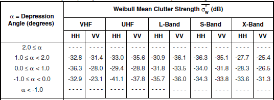
Trends in ![]() . Table 5.27 presents mean clutter strength
. Table 5.27 presents mean clutter strength ![]() for low-relief forest by frequency band, polarization, and depression angle and includes the number of measurements upon which each value of
for low-relief forest by frequency band, polarization, and depression angle and includes the number of measurements upon which each value of ![]() is based. The low-relief forest
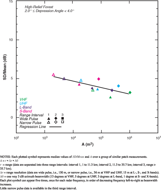
is based. The low-relief forest ![]() data of Table 5.27 are plotted in Figure 5.26. The main characteristics of the data in Figure 5.26 are similar to those of low-relief general mixed rural terrain shown in Figure 5.10 and discussed in Section 5.3.1.2. In particular, like the low-relief general mixed rural
data of Table 5.27 are plotted in Figure 5.26. The main characteristics of the data in Figure 5.26 are similar to those of low-relief general mixed rural terrain shown in Figure 5.10 and discussed in Section 5.3.1.2. In particular, like the low-relief general mixed rural ![]() data, the low-relief forest
data, the low-relief forest ![]() data show the v-shapes within frequency bands indicating strong effects from depression angle.
data show the v-shapes within frequency bands indicating strong effects from depression angle.
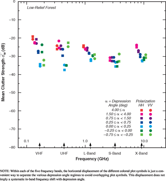
In Figure 5.26, the v-shape at X-band is particularly well-formed. Mean strength ![]() rises smoothly and uniformly with increasing depression angle through positive (i.e., left side of v-shape) depression angles from cyan (0° to 0.25°) to dark blue (0.25° to 0.75°) to purple (0.75° to 1.5°) to magenta (1.5° to 4°), and through negative (i.e., right side of v-shape) depression angles from cyan (0° to 0.25°) to dark green (0° to −0.25°) to intermediate green (–0.25° to −0.75°). This systematic behavior of increasing
rises smoothly and uniformly with increasing depression angle through positive (i.e., left side of v-shape) depression angles from cyan (0° to 0.25°) to dark blue (0.25° to 0.75°) to purple (0.75° to 1.5°) to magenta (1.5° to 4°), and through negative (i.e., right side of v-shape) depression angles from cyan (0° to 0.25°) to dark green (0° to −0.25°) to intermediate green (–0.25° to −0.75°). This systematic behavior of increasing ![]() with increasing positive or negative depression angle is to a significant extent caused by decreasing incidence of microshadowing with increasing depression angle in low-relief forest, although the intrinsic effect of increasing clutter strength with increasing illumination angle is also at work in these results. Similar systematic behavior with small changes in depression angle is observed in the Phase Zero X-band data (e.g., see Figures 1.9, 2.44, and 2.47). A very large amount of measurement data from many sites underlies these very well-formed X-band v-shapes, both for low-relief general mixed rural terrain in Figure 5.10 and for low-relief forest in Figure 5.26. A large amount of data is necessary for this systematic behavior with depression angle to emerge. In Figure 5.26, mean clutter strengths at L-band are very similar to those at X-band. At S-band, the low depression angle (i.e., cyan, dark green, dark blue)
with increasing positive or negative depression angle is to a significant extent caused by decreasing incidence of microshadowing with increasing depression angle in low-relief forest, although the intrinsic effect of increasing clutter strength with increasing illumination angle is also at work in these results. Similar systematic behavior with small changes in depression angle is observed in the Phase Zero X-band data (e.g., see Figures 1.9, 2.44, and 2.47). A very large amount of measurement data from many sites underlies these very well-formed X-band v-shapes, both for low-relief general mixed rural terrain in Figure 5.10 and for low-relief forest in Figure 5.26. A large amount of data is necessary for this systematic behavior with depression angle to emerge. In Figure 5.26, mean clutter strengths at L-band are very similar to those at X-band. At S-band, the low depression angle (i.e., cyan, dark green, dark blue) ![]() data are slightly weaker than at L- and X-band, but the high depression angle (i.e., magenta, purple) S-band data are much weaker than at L- and X-band. In fact, the high depression angle dependence from dark blue (0.25° to 0.75°) through purple (0.75° to 1.5°), magenta (1.5° to 4°), and red (> 4°) that exists in other bands in Figure 5.26 is completely lacking at S-band. That is, at high angles at S-band,
data are slightly weaker than at L- and X-band, but the high depression angle (i.e., magenta, purple) S-band data are much weaker than at L- and X-band. In fact, the high depression angle dependence from dark blue (0.25° to 0.75°) through purple (0.75° to 1.5°), magenta (1.5° to 4°), and red (> 4°) that exists in other bands in Figure 5.26 is completely lacking at S-band. That is, at high angles at S-band, ![]() does not rise with depression angle. This lack of depression angle dependence at high angles in S-band
does not rise with depression angle. This lack of depression angle dependence at high angles in S-band ![]() data from low-relief forest indicates that, with increasing angle, the forest is becoming increasingly absorptive of the RF energy at S-band. Looking across all five frequency bands in Figure 5.26, this increased absorptivity at S-band is made very evident by lower values of
data from low-relief forest indicates that, with increasing angle, the forest is becoming increasingly absorptive of the RF energy at S-band. Looking across all five frequency bands in Figure 5.26, this increased absorptivity at S-band is made very evident by lower values of ![]() (i.e., an S-band dip), particularly at the higher angles of illumination.
(i.e., an S-band dip), particularly at the higher angles of illumination.
The grazing incidence, 0° to 0.25° (cyan) low-relief forest ![]() results in Figure 5.26 show little variation with frequency band. At L-band and X-band, these results are at about the −32 dB level, with S-band slightly lower; at VHF and UHF, these results are at about the −35 dB level. However, in the lower bands there is a much larger increase from the cyan, 0° to 0.25° results to the dark blue, 0.25° to 0.75° results than in the upper bands. This increase is about 8 dB at VHF and UHF, about 4 dB at L-band, and about 3 dB at S- and X-band. This changing difference may indicate that there is a more rapid onset of illumination with increasing depression angle (or, in other words, that microshadow disappears faster) in the lower bands than in the upper bands, possibly due to increased diffractive effects at the lower frequencies.
results in Figure 5.26 show little variation with frequency band. At L-band and X-band, these results are at about the −32 dB level, with S-band slightly lower; at VHF and UHF, these results are at about the −35 dB level. However, in the lower bands there is a much larger increase from the cyan, 0° to 0.25° results to the dark blue, 0.25° to 0.75° results than in the upper bands. This increase is about 8 dB at VHF and UHF, about 4 dB at L-band, and about 3 dB at S- and X-band. This changing difference may indicate that there is a more rapid onset of illumination with increasing depression angle (or, in other words, that microshadow disappears faster) in the lower bands than in the upper bands, possibly due to increased diffractive effects at the lower frequencies.
In the pure low-relief forest ![]() data of Figure 5.26, significant multipath is not generally at work to reduce the low-angle, cyan (0° to 0.25°) and dark blue (0.25° to 0.75°)
data of Figure 5.26, significant multipath is not generally at work to reduce the low-angle, cyan (0° to 0.25°) and dark blue (0.25° to 0.75°) ![]() results to much lower levels at VHF and UHF. In contrast, multipath does have significant influence in partially open, general mixed rural terrain to reduce the cyan and dark blue, VHF and UHF
results to much lower levels at VHF and UHF. In contrast, multipath does have significant influence in partially open, general mixed rural terrain to reduce the cyan and dark blue, VHF and UHF ![]() results of Figure 5.10 to lower levels. The existence of multipath in the low-relief general mixed rural
results of Figure 5.10 to lower levels. The existence of multipath in the low-relief general mixed rural ![]() results of Figure 5.10 is particularly evidenced by the fact that the low-angle cyan (0° to 0.25°) and dark blue (0.25° to 0.75°)
results of Figure 5.10 is particularly evidenced by the fact that the low-angle cyan (0° to 0.25°) and dark blue (0.25° to 0.75°) ![]() results increase strongly with increasing frequency, VHF through L-band; a comparable strong uniform increase is lacking in the low-relief forest
results increase strongly with increasing frequency, VHF through L-band; a comparable strong uniform increase is lacking in the low-relief forest ![]() results of Figure 5.26.
results of Figure 5.26.
The v-shaped clusters in Figure 5.26 showing low-relief forest ![]() data are significantly lower in each frequency band than the v-shaped clusters in Figure 5.24 showing high-relief forest
data are significantly lower in each frequency band than the v-shaped clusters in Figure 5.24 showing high-relief forest ![]() data. That is, in forested terrain, which constitutes a relatively simple, diffusely reflective scattering surface uncomplicated by questions of significant coherent reflection, separating terrain in two regimes of relief, high (terrain slopes > 2°) and low (terrain slopes < 2°), results in significant separation of mean clutter strengths; and in each regime of relief, the influence of microshadowing in low-angle clutter results in strong effects of depression angle on mean clutter strength. As expected, these effects of depression angle are more significant in low-relief than in high-relief forest terrain because the increased terrain slopes in high-relief terrain reduce the amount of microshadowing.
data. That is, in forested terrain, which constitutes a relatively simple, diffusely reflective scattering surface uncomplicated by questions of significant coherent reflection, separating terrain in two regimes of relief, high (terrain slopes > 2°) and low (terrain slopes < 2°), results in significant separation of mean clutter strengths; and in each regime of relief, the influence of microshadowing in low-angle clutter results in strong effects of depression angle on mean clutter strength. As expected, these effects of depression angle are more significant in low-relief than in high-relief forest terrain because the increased terrain slopes in high-relief terrain reduce the amount of microshadowing.
Section 5.4.3.1 compared low-angle clutter statistics from high-relief forest and farmland. Comparison between Figures 5.20 and 5.26 (and Tables 5.19 and 5.27) indicates that low-relief forest ![]() ranges from being substantially greater than low-relief farmland
ranges from being substantially greater than low-relief farmland ![]() to being nearly equivalent to low-relief farmland
to being nearly equivalent to low-relief farmland ![]() , depending on frequency band and depression angle regime. More specifically, the amount by which low-relief forest
, depending on frequency band and depression angle regime. More specifically, the amount by which low-relief forest ![]() exceeds low-relief farmland
exceeds low-relief farmland ![]() by frequency band and depression angle regime is: at VHF, from 20 dB at high angle to 6 dB at low angle; at UHF, from 10 dB at high angle to 6 dB at low angle; at L-band and X-band, by 6 or 7 dB at high angle to near equivalence at low angle; and at S-band, near equivalence at all angles.
by frequency band and depression angle regime is: at VHF, from 20 dB at high angle to 6 dB at low angle; at UHF, from 10 dB at high angle to 6 dB at low angle; at L-band and X-band, by 6 or 7 dB at high angle to near equivalence at low angle; and at S-band, near equivalence at all angles.
In broad measure, polarization differences are very small in the low-relief forest ![]() data of Figure 5.26. There is a slight overall bias whereby
data of Figure 5.26. There is a slight overall bias whereby ![]() is slightly greater than
is slightly greater than ![]() in all depression angle regimes at S- and X-band, and, except for −0.25° to −0.75°, also at UHF; less generally true at VHF and L-band. The somewhat larger polarization differences in the −0.25° to −0.75° depression angle regime reflect the fact that little data are available in this regime.
in all depression angle regimes at S- and X-band, and, except for −0.25° to −0.75°, also at UHF; less generally true at VHF and L-band. The somewhat larger polarization differences in the −0.25° to −0.75° depression angle regime reflect the fact that little data are available in this regime.
Uncertain Outliers. In Figure 5.26 showing ![]() results for low-relief forest, there are relatively little data available in the light green, −0.25° to −0.75° depression angle regime (viz., 39 measured clutter histograms from four clutter patches; see Table 5.24). Nevertheless, in the three upper frequency bands these light green
results for low-relief forest, there are relatively little data available in the light green, −0.25° to −0.75° depression angle regime (viz., 39 measured clutter histograms from four clutter patches; see Table 5.24). Nevertheless, in the three upper frequency bands these light green ![]() results fall in quite closely with the cyan and dark green results, and show a trend of increasing
results fall in quite closely with the cyan and dark green results, and show a trend of increasing ![]() with increasing negative depression angle, cyan to dark green to light green. However, at VHF and UHF, larger differences occur between the light green and dark green
with increasing negative depression angle, cyan to dark green to light green. However, at VHF and UHF, larger differences occur between the light green and dark green ![]() results than in the upper bands, and the relative behavior of the light green and dark green results with respect to each other and with respect to the cyan results is more erratic. The light green results largely come from three patches (patch 39 at the Cold Lake measurement site and patches 46 and 47 at the Woking measurement site) which exist at relatively long ranges (33 to 47 km) with some mix of open and forested terrain occurring between the radar and the clutter patches. Thus some degree of multipath may be occurring in these light green VHF and UHF measurements, possibly acting to reduce clutter strength at VHF and to augment clutter strength at UHF. This possibility of multipath in the light green results does not explain why the dark green results, which are based on many more measurements than the light green results, are relatively strong at VHF and relatively weak at UHF. This discussion brings forward the fact that classification of a clutter patch as forest does not necessarily imply that all of the terrain between the patch and the radar is forested.
results than in the upper bands, and the relative behavior of the light green and dark green results with respect to each other and with respect to the cyan results is more erratic. The light green results largely come from three patches (patch 39 at the Cold Lake measurement site and patches 46 and 47 at the Woking measurement site) which exist at relatively long ranges (33 to 47 km) with some mix of open and forested terrain occurring between the radar and the clutter patches. Thus some degree of multipath may be occurring in these light green VHF and UHF measurements, possibly acting to reduce clutter strength at VHF and to augment clutter strength at UHF. This possibility of multipath in the light green results does not explain why the dark green results, which are based on many more measurements than the light green results, are relatively strong at VHF and relatively weak at UHF. This discussion brings forward the fact that classification of a clutter patch as forest does not necessarily imply that all of the terrain between the patch and the radar is forested.
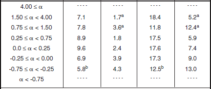
Shape Parameter aw. Table 5.28 provides the Weibull shape parameter aw and associated information for clutter amplitude distributions in low-relief forest terrain. Each pair of aw numbers in Table 5.28 comes from a scatter plot of sd/mean or mean/median vs spatial resolution A. Figure 5.27 shows the sd/mean scatter plot for the 0.0° to 0.25° depression angle regime. As in high-relief forest, spreads in clutter amplitude distributions continue to be relatively low in low-relief forest, compared with other terrain types. There continues to be a strong trend of decreasing spread with increasing cell size A, and a weak trend of decreasing spread with increasing depression angle. Spreads in low-relief forest are similar to spreads in high-relief forest. In Figure 5.27, the five VHF data points separate out as being of less spread than shown in the other bands and as being of little variation with A.
TABLE 5.28
Shape Parameter aw and Ratios of Standard Deviation-to-Mean (SD/Mean) and Mean-to-Median for Low-Relief Forest, by Spatial Resolution A and Depression Angle*
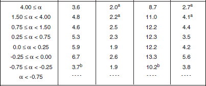
aFootnoted values apply at A = 105m2, not 106m2.
bFootnoted values apply at A = 105m2, not 103m2.
*Table 5.24 defines the population of terrain patches and measurements upon which these data are based.
5.4.4 SHRUBLAND TERRAIN
Less discussion is provided for following terrain types in Section 5.4—shrubland, grassland, wetland, desert, mountains—than was provided for foregoing terrain types of urban, agricultural, and forest. The reason for this is to avoid redundant discussion—many of the points to be made have already been dealt with in previous discussions. Uncertain outliers continue to be indicated with open plot symbols for the terrain types that follow, although they are not discussed in the text.
The land cover classification system utilized provides rangeland as a major land cover category (see Table 2.1). Within rangeland, there are three specific subcategories—herbaceous rangeland, shrubby rangeland, and mixed herbaceous/shrubby rangeland. Hereafter, pure herbaceous rangeland clutter patches are referred to as grassland, and patches classified as shrubby or herbaceous/shrubby mixtures are referred to as shrubland. Forest, shrubland, and grassland thus comprise three land cover classes involving natural vegetation for which the height of the vegetation significantly decreases from forest to shrubland to grassland. As will be seen, this decrease in vegetation height results in significantly differing clutter characteristics from these three terrain types.
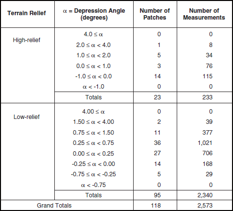
Table 5.29 shows the statistical populations underlying the shrubland clutter modeling information to follow. These populations are relatively low, involving only 1,030 measured clutter amplitude distributions from 51 patches. The high-relief shrubland patches come from three different sites, the low-relief shrubland patches from seven different sites.
TABLE 5.29
Numbers of Terrain Patches and Measured Clutter Histograms for Shrubland, by Relief and Depression Anglea,b,c
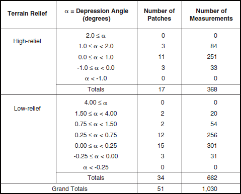
aA single (primary) classifier only is sufficient to describe these patches.
bA terrain patch is a land surface macroregion usually several kms on a side (median patch area = 12.62 km2).
cA measured clutter histogram contains all of the temporal (pulse by pulse) and spatial (resolution cell by resolution cell) clutter samples obtained in a given measurement of a terrain patch. A terrain patch was usually measured many times (nominally 20) as RF frequency (5), polarization (2), and range resolution (2) were varied over the Phase One radar parameter matrix.
5.4.4.1 HIGH-RELIEF SHRUBLAND
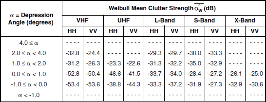
Clutter modeling information for high-relief shrubland is given in Tables 5.30 and 5.31 and Figures 5.28 and 5.29. Mean clutter strengths at VHF and UHF in Figure 5.28 vary somewhat erratically. Mean strengths at L- and S-bands cluster more tightly. In general, high-relief shrubland mean clutter strengths in Figure 5.28 are relatively invariant with frequency, VHF to S-band, but increase at X-band. The X-band data are also tightly clustered by polarization and depression angle. Comparison with Figure 5.24 shows that mean clutter strength in high-relief forest is generally much greater than in high-relief shrubland, with the differences most pronounced in the lower bands and least at X-band. Comparison with Figure 5.18 shows that mean clutter strength in high-relief agricultural terrain is overall somewhat similar to that in high-relief shrubland.
TABLE 5.30
Mean Clutter Strength ![]() , and Number of Measurements for High-Relief Shrubland, by Frequency Band, Polarization, and Depression Anglea
, and Number of Measurements for High-Relief Shrubland, by Frequency Band, Polarization, and Depression Anglea
aTable 5.29 defines the population of terrain patches upon which these data are based.
TABLE 5.31
Shape Parameter aw and Ratios of Standard Deviation-to-Mean (SD/Mean) and Mean-to-Median for High-Relief Shrubland, by Spatial Resolution A and Depression Anglea
aTable 5.29 defines the population of terrain patches and measurements upon which these data are based.
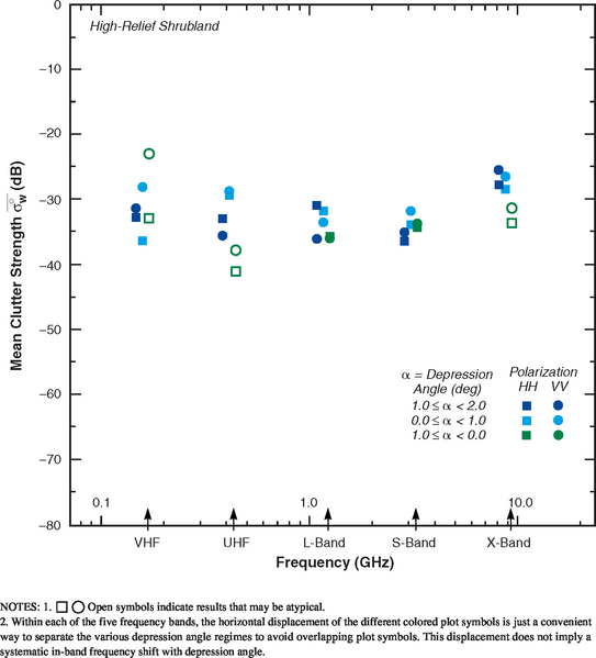
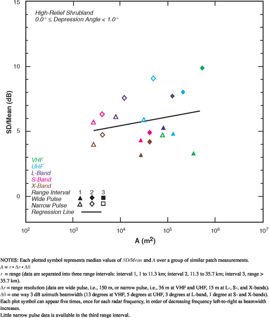
FIGURE 5.29 Ratio of standard deviation-to-mean (SD/Mean) vs radar spatial resolution A for high-relief shrubland with depression angle between 0.0 and 1.0 degrees.
Table 5.31 indicates relatively little trend of decreasing spread with increasing cell size A, for high-relief shrubland, in contrast to most other terrain types. In particular, in the 0° to 1° depression angle regime, Figure 5.29 shows extreme variability in the scatter plot of sd/mean vs A, with a regression line in this case actually showing gradually increasing spread with A.
This indicates that high-relief shrubland is extremely heterogeneous in character—the shrubland is not a homogeneous vegetative cover of uniform height and density.
5.4.4.2 LOW-RELIEF SHRUBLAND
Clutter modeling information for low-relief shrubland is given in Tables 5.32 and 5.33 and Figures 5.30 and 5.31. Figure 5.30 indicates that mean clutter strength in low-relief shrubland has strong, well-behaved trends of variation with frequency and depression angle. In the 0° to 0.25° degree depression angle regime, mean clutter strengths rise from −52 or −54 dB at UHF to −33 or −34 dB at X-band; this 20 dB rise is due to decreasing multipath propagation loss with increasing frequency, UHF to X-band. The X-band data show a particularly well-behaved trend with depression angle rising from −33 dB at low angle to −23 dB at high angle. The VHF mean strengths at low angle (cyan) being stronger than at UHF indicates much stronger intrinsic σ° at VHF than UHF, enough to overcome increased multipath propagation loss at VHF. In general these low-relief shrubland data are much weaker than low-relief forest except at X-band; they are also generally weaker than low-relief farmland.
TABLE 5.32
Mean Clutter Strength ![]() and Number of Measurements for Low-Relief Shrubland, by Frequency Band, Polarization, and Depression Anglea
and Number of Measurements for Low-Relief Shrubland, by Frequency Band, Polarization, and Depression Anglea

aTable 5.29 defines the population of terrain patches upon which these data are based.
TABLE 5.33
Shape Parameter aw and Ratios of Standard Deviation-to-Mean (SD/Mean) and Mean-to-Median for Low-Relief Shrubland, by Spatial Resolution A and Depression Angle*
aFootnoted values apply at A = 105 m2, not 103 m2.
*Table 5.29 defines the population of terrain patches and measurements upon which these data are based.
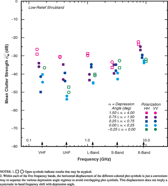
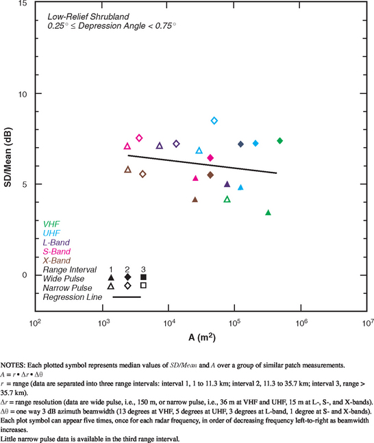
FIGURE 5.31 Ratio of standard deviation-to-mean (SD/Mean) vs radar spatial resolution A for low-relief shrubland with depression angle between 0.25 and 0.75 degrees.
Table 5.33 and Figure 5.31 show that spreads in low-relief shrubland are somewhat better behaved than in high-relief shrubland—there are at least consistent trends of decreasing spread with increasing A, but the trends are weaker than in other terrain types. The scatter plot of Figure 5.31 for low-relief shrubland continues to show extreme variability, although the weak regression line shown is of the expected slope.
5.4.5 GRASSLAND TERRAIN
Table 5.34 shows the statistical populations underlying the grassland clutter modeling information to follow. As with shrubland, the high-relief grassland populations remain small, but the low-relief grassland populations are significantly higher. High-relief grassland patches come from six different sites, the low-relief grassland patches from nine different sites.
TABLE 5.34
Numbers of Terrain Patches and Measured Clutter Histograms for Grassland, by Relief and Depression Anglea,b,c
aA single (primary) classifier only is sufficient to describe these patches.
bA terrain patch is a land surface macroregion usually several kms on a side (median patch area = 12.62 km2).
cA measured clutter histogram contains all of the temporal (pulse by pulse) and spatial (resolution cell by resolution cell) clutter samples obtained in a given measurement of a terrain patch. A terrain patch was usually measured many times (nominally 20) as RF frequency (5), polarization (2), and range resolution (2) were varied over the Phase One radar parameter matrix.
5.4.5.1 HIGH-RELIEF GRASSLAND
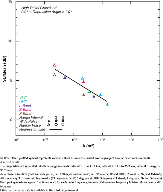
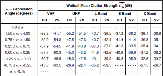
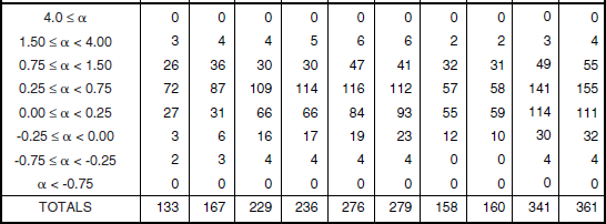
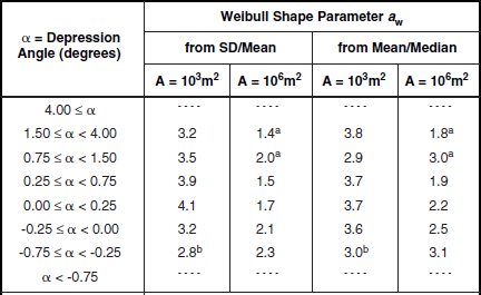
Clutter modeling information for high-relief grassland is given in Tables 5.35 and 5.36 and Figures 5.32 and 5.33. Much of the high-relief grassland mean clutter strength data is in the 0° to 1° or 0° to −1° depression angle regimes. In contrast to high-relief shrubland, mean clutter strength in high-relief grassland shows a strong trend of increasing strength with increasing frequency, VHF to X-band; and is generally much weaker than high-relief shrubland, particularly in the lower bands. Also in marked contrast to high-relief shrubland, the information describing spread in clutter amplitude distributions in high-relief grassland in Table 5.36 and Figure 5.33 is well behaved, showing strong trends of decreasing spread with increasing cell size A, and a weaker trend of decreasing spread with increasing depression angle. The scatter plot of Figure 5.33 shows a strong trend of decreasing sd/mean with increasing A and little variability about its regression line, in marked contrast with the extreme shrubland scatter shown in Figures 5.29 and 5.31.
TABLE 5.35
Mean Clutter Strength ![]() and Number of Measurements for High-Relief Grassland, by Frequency Band, Polarization, and Depression Anglea
and Number of Measurements for High-Relief Grassland, by Frequency Band, Polarization, and Depression Anglea
aTable 5.34 defines the population of terrain patches upon which these data are based.
TABLE 5.36
Shape Parameter aw and Ratios of Standard Deviation-to-Mean (SD/Mean) and Mean-to-Median for High-Relief Grassland, by Spatial Resolution A and Depression Angle*
aFootnoted values apply at A = 105 m2, not 103 m2.
bFootnoted values apply at A = 105 m2, not 106 m2.
*Table 5.34 defines the population of terrain patches and measurements upon which these data are based.
5.4.5.2 LOW-RELIEF GRASSLAND
Clutter modeling information for low-relief grassland is given in Tables 5.37 and 5.38 and Figures 5.34 and 5.35. As in high-relief grassland, the low-relief grassland mean clutter strength data of Figure 5.34 continue to show a strong trend of increasing strength with increasing frequency, VHF to X-band. There is little variation in these results with depression angle. Mean clutter strength in low-relief grassland is somewhat weaker than in high-relief grassland in every band. Comparison with low-relief shrubland is interesting in that mean clutter strength in low-relief shrubland has such a strong dependency on depression angle in every band, whereas in low-relief grassland it has none. At higher angles, low-relief shrubland is stronger than low-relief grassland in every band; but at grazing incidence the picture is more complicated, with grassland equal or stronger in the upper bands, but shrubland stronger at VHF. The spreads in clutter amplitude distributions in low-relief grassland given in Table 5.38 and Figure 5.35, as in high-relief grassland, continue to show strong trends of decreasing spread with increasing cell size A. The scatter plot of Figure 5.35 shows strong correlation about the regression line.
TABLE 5.37
Mean Clutter Strength ![]() and Number of Measurements for Low-Relief Grassland, by Frequency Band, Polarization, and Depression Anglea
and Number of Measurements for Low-Relief Grassland, by Frequency Band, Polarization, and Depression Anglea
aTable 5.34 defines the population of terrain patches upon which these data are based.
TABLE 5.38
Shape Parameter aw and Ratios of Standard Deviation-to-Mean (SD/Mean) and Mean-to-Median for Low-Relief Grassland, by Spatial Resolution A and Depression Angle*
aFootnoted values apply at A = 105 m2, not 106 m2.
bFootnoted values apply at A = 105 m2, not 103 m2.
*Table 5.34 defines the population of terrain patches and measurements upon which these data are based.
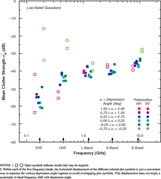
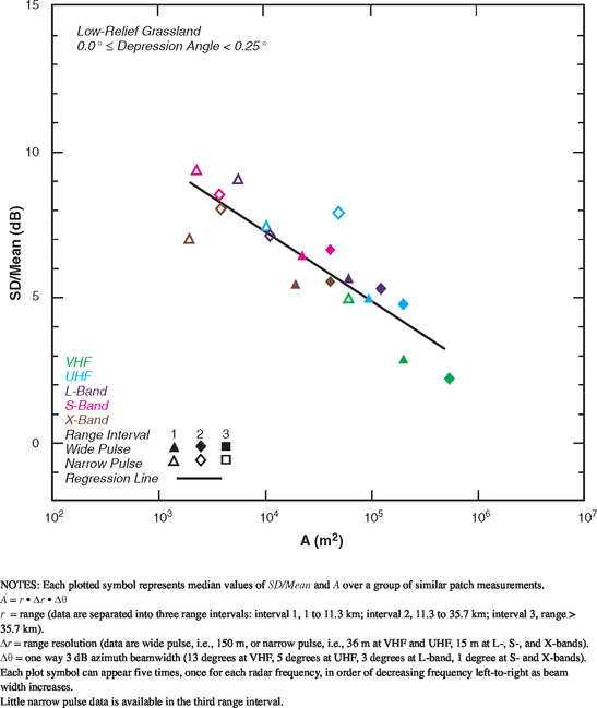
FIGURE 5.35 Ratio of standard deviation-to-mean (SD/Mean) vs radar spatial resolution A for low-relief grassland with depression angle between 0.0 and 0.25 degrees.
Shrubland vs Grassland. The classification system separating shrubland from grassland as specific subcategories of general rangeland has found significant differences in the low-angle clutter characteristics of shrubland and grassland. Shrubland shows a strong trend of mean strength on depression angle (Figure 5.30), but is poorly behaved in its spread characteristics (Figure 5.31), whereas grassland shows little or no variation of mean strength with depression angle (Figure 5.34), but is well behaved in its spread characteristics with strong trends of decreasing spread with increasing cell size A (Figure 5.35). It is interesting to compare and contrast the grassland and shrubland mean clutter strength data provided here in Chapter 5 with the well-behaved Vananda East repeat sector mean clutter strength characteristic shown in Figure 3.6 in Chapter 3—the Vananda East repeat sector was transitional between grassland (LC = 31) and shrubland (LC = 32) in low-relief terrain with undulating (LF = 3) and hummocky (LF = 5) components; see Figure 3.6.
5.4.6 WETLAND TERRAIN
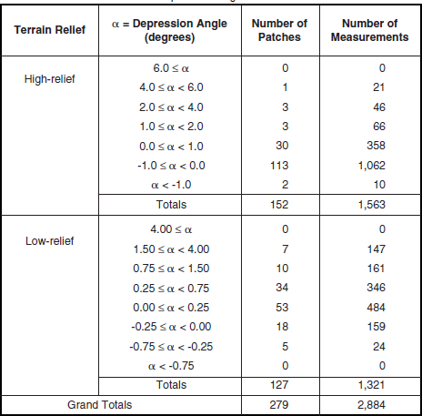
Table 5.39 shows the statistical population underlying the wetland clutter modeling information to follow. This population comprises 447 measured clutter amplitude distributions from 17 clutter patches at three different sites. Many of these measurements occurred at Big Grass Marsh, Manitoba, which was visited by Phase One in winter weather (see Chapter 3, Section 3.4.1.5). All wetland clutter patches were of “level” landform classification.
TABLE 5.39
Numbers of Terrain Patches and Measured Clutter Histograms for Wetland, by Depression Anglea,b,c
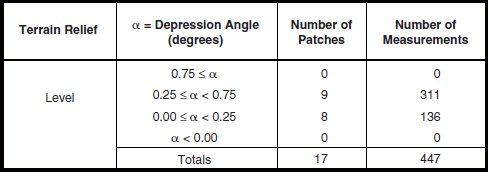
aA single (primary) classifier only is sufficient to describe these patches.
bA terrain patch is a land surface macroregion usually several kms on a side (median patch area = 12.62 km2).
cA measured clutter histogram contains all of the temporal (pulse by pulse) and spatial (resolution cell by resolution cell) clutter samples obtained in a given measurement of a terrain patch. A terrain patch was usually measured many times (nominally 20) as RF frequency (5), polarization (2), and range resolution (2) were varied over the Phase One radar parameter matrix.
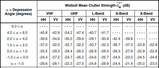
Clutter modeling information for wetland is provided in Tables 5.40 and 5.41 and Figures 5.36 and 5.37. As shown in Figure 5.36, mean clutter strength for wetland is very weak—in fact, it is the weakest clutter strength in every band of any of the terrain types examined. The results of Figure 5.37 correspond quite closely with the Big Grass Marsh repeat sector results shown in Figure 3.8 in Chapter 3. Mean clutter strength is particularly weak at VHF and UHF in Figure 5.36, hovering in the neighborhood of −67 to −72 dB. Although very weak, these are accurate measured clutter strength numbers unaffected by Phase One sensitivity limitations and noise corruption (see Appendix 3.C for examples of accurate weak clutter computation at Big Grass Marsh). The wetland mean strength data show a strong trend of increasing strength with increasing frequency, UHF to X-band—obviously due to multipath propagation, and a weaker trend in most bands of increasing strength with increasing depression angle between 0° to 0.25° and 0.25° to 0.75°—the only depression angle regimes in which data exist for wetland. The fact that VHF mean clutter strengths are somewhat stronger than at UHF indicates that intrinsic σ° is significantly greater at VHF than UHF for wetland, a result previously seen in repeat sector data in Chapter 3.
TABLE 5.40
Mean Clutter Strength ![]() and Number of Measurements for Wetland, by Frequency Band, Polarization, and Depression Anglea
and Number of Measurements for Wetland, by Frequency Band, Polarization, and Depression Anglea
aTable 5.39 defines the population of terrain patches upon which these data are based.
TABLE 5.41
Shape Parameter aw and Ratios of Standard Deviation-to-Mean (SD/Mean) and Mean-to-Median for Wetland, by Spatial Resolution A and Depression Angle*
aFootnoted values apply at A = 105 m2, not 106 m2.
*Table 5.39 defines the population of terrain patches and measurements upon which these data are based.
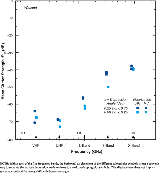
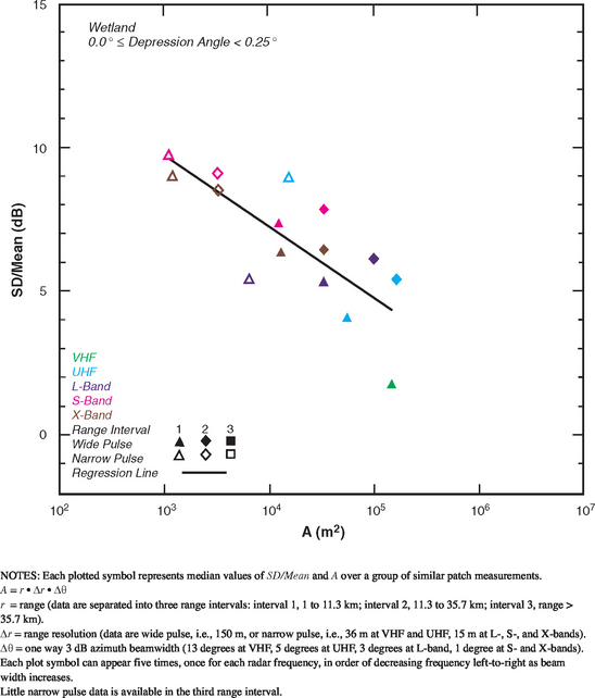
FIGURE 5.37 Ratio of standard deviation-to-mean (SD/Mean) vs radar spatial resolution A for wetland with depression angle between 0.0 and 0.25 degrees.
Table 5.41 and Figure 5.37 indicate strong trends of decreasing spread in level wetland clutter amplitude distributions with increasing cell size A. In this respect, level wetland is like low-relief grassland (compare Figure 5.37 with Figure 5.35).
5.4.7 DESERT TERRAIN
Desert terrain does not explicitly appear in the land cover and landform terrain classification systems employed herein (see Section 2.2.3, Tables 2.1 and 2.2). A criterion utilized to specify desert clutter within the Phase One measurement database is that the desert clutter must come from two Phase One sites—Booker Mountain, Nevada, and Knolls, Utah—that were situated in typical western desert terrain (see Section 3.4.1.5). Booker Mountain was a high site; Knolls was a low site. At both sites, low-relief desert valleys were surrounded by steep terrain at much higher elevations. The low-relief valley floors were typically covered with sparse desert vegetation, but with occasional barren dry lake beds or salt flats. The surrounding high-relief terrain had occasional occurrences of patches of trees, principally on steep slopes at higher elevations. A further criterion for a clutter patch to be accepted as desert at either of these two sites is that, if low relief, its land cover classification be predominantly rangeland or barren; if high-relief, a component of trees was also allowed. Table 5.42 indicates that, for desert terrain thusly defined, there are available 2,884 measured Phase One clutter amplitude distributions from 279 desert clutter patches. These desert patches and histograms are approximately equally distributed between high-relief patches and low-relief patches. Repeat sector desert clutter measurements at Booker Mountain and Knolls were previously discussed in Chapter 3, Section 3.4.1.5 (in particular, see Figure 3.37).
TABLE 5.42
Numbers of Terrain Patches and Measured Clutter Histograms for Desert, by Relief and Depression Anglea,b,c
aAmerican Intermontane West terrain. Knolls and Booker Mountain sites. Predominantly with shrubby desert vegetation or barren.
bA terrain patch is a land surface macroregion usually several kms on a side (median patch area = 12.62 km2).
cA measured clutter histogram contains all of the temporal (pulse by pulse) and spatial (resolution cell by resolution cell) clutter samples obtained in a given measurement of a terrain patch. A terrain patch was usually measured many times (nominally 20) as RF frequency (5), polarization (2), and range resolution (2) were varied over the Phase One radar parameter matrix.
5.4.7.1 HIGH-RELIEF DESERT
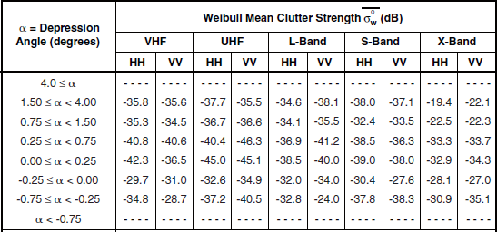
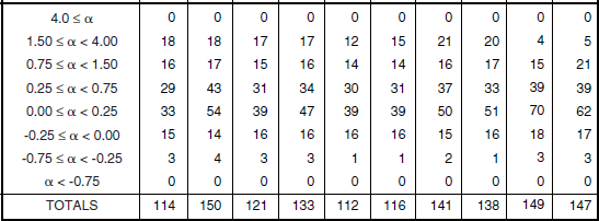
Clutter modeling information for high-relief desert is given in Tables 5.43 and 5.44 and Figures 5.38 and 5.39. In Figure 5.38, mean clutter strengths at low angles (cyan and green) are observed to be relatively frequency independent, VHF to S-band—but perhaps a little stronger at X-band. In this respect these data are very different from high-relief forest, even though high-relief desert terrain has significant occurrences of trees. In the lower bands in Figure 5.38 there is an unusual strong, inverse dependence with depression angle wherein clutter strengths decrease with increasing depression angle, from cyan through dark blue, and purple, to magenta. The reason for this unusual trend in these data is as follows. High-relief desert terrain observed at low angles comes from either steep surrounding mountains at the low Knolls site or steep neighboring mountain peaks at the high Booker Mountain site. Such steep terrain observed at near broadside incidence (i.e., low depression angle) results in strong clutter. In contrast, high-relief desert observed at high depression angle comes from terrain of lower elevations—albeit of high relief—at the higher Booker Mountain site. Looking down at surrounding, lower elevation, mountainous patches provides significantly weaker clutter in Figure 5.38 (dark blue, purple, magenta) than when surrounding mountainous patches at more nearly equal or even greater elevation are viewed nearer broadside incidence (cyan, dark green). The X-band data in Figure 5.38 do not show this trend, or any trend with depression angle—rather, they form a very tight cluster. In Section 5.4.8 which follows, a similar inverse trend of mean clutter strength with depression angle for mountain terrain is observed, and for the same reasons.
TABLE 5.43
Mean Clutter Strength ![]() and Number of Measurements for High-Relief Desert, by Frequency Band, Polarization, and Depression Anglea
and Number of Measurements for High-Relief Desert, by Frequency Band, Polarization, and Depression Anglea
aTable 5.42 defines the population of terrain patches upon which these data are based.
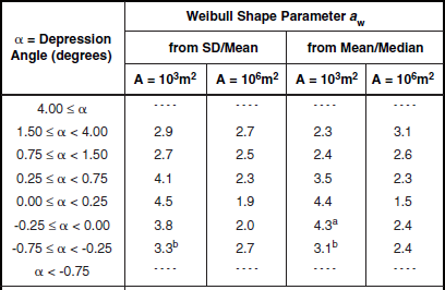
TABLE 5.44
Shape Parameter aw and Ratios of Standard Deviation-to-Mean (SD/Mean) and Mean-to-Median for High-Relief Desert, by Spatial Resolution A and Depression Angle*
aFootnoted values apply at A = 105 m2, not 103 m2.
*Table 5.42 defines the population of terrain patches and measurements upon which these data are based.
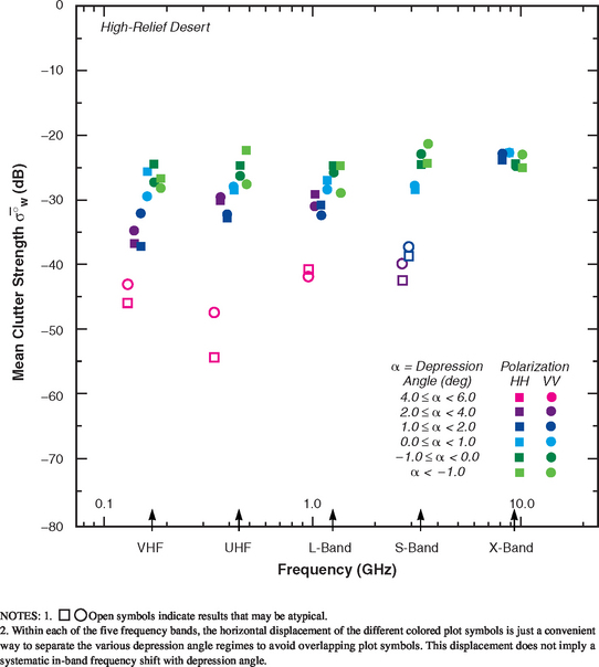
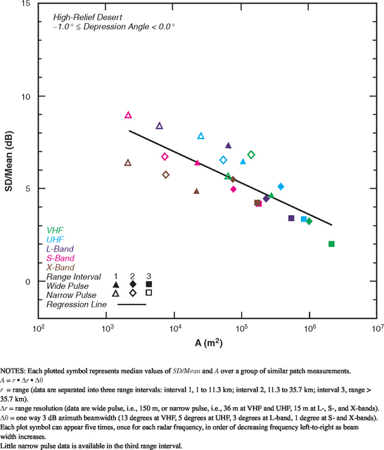
FIGURE 5.39 Ratio of standard deviation-to-mean (SD/Mean) vs radar spatial resolution A for high-relief desert with depression angle between −1.0 and 0.0 degrees.
Table 5.44 and Figure 5.39 provide information on the spread of clutter amplitude distributions in high-relief desert terrain. There is seen to be a strong general trend of decreasing spread with increasing cell size A; there is also a weaker trend whereby spread diminishes with increasing depression angle.
5.4.7.2 LOW-RELIEF DESERT
Clutter modeling information for low-relief desert is given in Tables 5.45 and 5.46 and Figures 5.40 and 5.41. Comparison of Figure 5.40 with Figure 5.38 shows mean clutter strength in low-relief desert to be generally very much weaker than in high-relief desert. Also, in marked contrast to high-relief desert, in low-relief desert there is a strong, positive, trend—not inverse here—of increasing clutter strength with increasing depression angle. This expected trend indicates that clutter strength from low-relief desert valley floors is stronger as observed at high depression angle from Booker Mountain, but is weaker as observed at low depression angle from Knolls.
TABLE 5.45
Mean Clutter Strength ![]() and Number of Measurements for Low-Relief Desert, by Frequency Band, Polarization, and Depression Anglea
and Number of Measurements for Low-Relief Desert, by Frequency Band, Polarization, and Depression Anglea
aTable 5.42 defines the population of terrain patches upon which these data are based.
TABLE 5.46
Shape Parameter aw and Ratios of Standard Deviation-to-Mean (SD/Mean) and Mean-to-Median for Low-Relief Desert, by Spatial Resolution A and Depression Angle*
aFootnoted values apply at A = 104 m2, not 103 m2.
bFootnoted values apply at A = 105 m2, not 103 m2.
*Table 5.42 defines the population of terrain patches and measurements upon which these data are based.
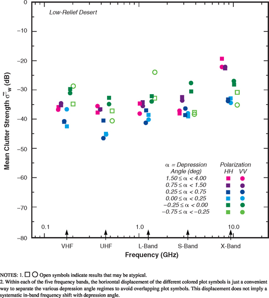
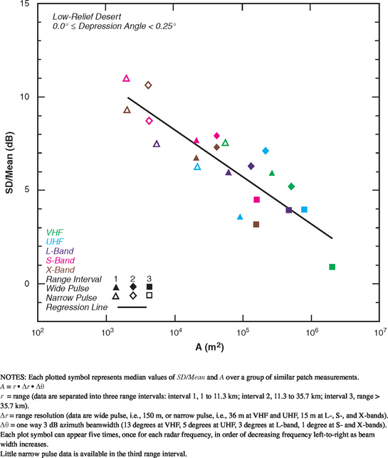
FIGURE 5.41 Ratio of standard deviation-to-mean (SD/Mean) vs radar spatial resolution A for low-relief desert with depression angle between 0.0 and 0.25 degrees.
A number of other interesting observations may be made of the low-relief desert data of Figure 5.40. First note that at low positive depression angles (cyan, dark blue), mean clutter strength is relatively invariant with frequency band, VHF to X-band (a little weaker at UHF, a little stronger at X-band). Furthermore, at higher angles (purple, magenta), mean clutter strength (although generally somewhat higher than at low angles) is also remarkably invariant with frequency, in this case VHF to S-band, but jumps ∼15 dB in clutter strength, S-band to X-band. This remarkable increase in mean clutter strength from S-band to X-band in high-angle data, and from low angle to high angle in X-band data, when looking down at high angle to a low-relief desert valley floor, was discussed earlier in the repeat sector results of Chapter 3 (Sections 3.4.1.5 and 3.4.2). In these survey data of Chapter 5, looking down at desert vegetation at high angle at X-band is even somewhat stronger than looking down at forest vegetation at high angle at X-band (see Figure 5.26), although otherwise mean clutter strength in low-relief forest is generally much greater than mean clutter strength in low-relief desert. This unusually strong, X-band only and high angle only, mean clutter strength of low-relief desert is even marginally higher than the corresponding mean strength in high-relief desert (see Figure 5.38). Finally, in Figure 5.40, note that mean clutter strength in low-relief desert at low negative depression angle (dark green) is relatively frequency invariant and relatively strong in all bands, VHF to X-band. For the most part, these data come from the higher terrain surrounding the valley at Knolls.
Table 5.46 and Figure 5.41 show clutter modeling information for spreads of clutter amplitude distributions in low-relief desert. These data are similar to those in high-relief desert, with strong trends of decreasing spread with increasing cell size A and a weaker trend of decreasing spread with increasing depression angle. That is, whereas first moment mean clutter strengths of high-relief and low-relief desert are quite different (e.g., exhibit opposite trends with depression angle), second moments (i.e., spreads) in clutter amplitude distributions of high- and low-relief desert are quite similar.
5.4.7.3 LEVEL DESERT
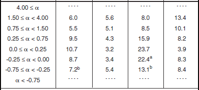
Level desert is a subcategory of low-relief desert. Level desert clutter patches are required to be of level landform (see Table 2.2) and of either rangeland or barren land cover (see Table 2.1). Table 5.47 indicates the availability of 537 measured Phase One clutter amplitude distributions from 38 level desert clutter patches. This subset represents about one-third of the available measurements for low-relief desert (see Table 5.42). Clutter modeling information for level desert is provided in Tables 5.48 and 5.49 and Figures 5.42 and 5.43. As in low-relief desert, the mean clutter strength data for level desert in Figure 5.42 continue to show a strong trend of increasing strength with increasing depression angle in each band—here the low angle data (cyan, dark blue) are much weaker, with a significant multipath-induced trend of increasing strength with frequency, UHF to X-band. As with wetland (see Figure 5.36), this multipath trend in the low angle data does not extend to VHF, indicating (as with wetland and low-relief shrubland) much greater intrinsic σ°’s in low angle VHF level desert data than at UHF (enough greater to overcome the increased multipath loss at VHF). Although weak and similar to wetland results, the low angle (cyan, dark blue) level desert results in Figure 5.42 are not as weak as the level wetland results of Figure 5.36.
TABLE 5.47
Numbers of Terrain Patches and Measured Clutter Histograms for Level Desert, by Depression Anglea,b,c
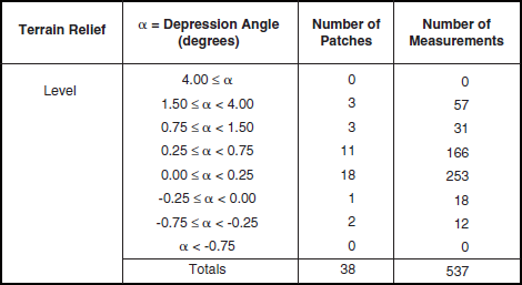
aAmerican Intermontane West terrain. Knolls and Booker Mountain sites. Predominantly with shrubby desert vegetation or barren. Level is included within low-relief.
bA terrain patch is a land surface macroregion usually several kms on a side (median patch area = 12.62 km2).
cA measured clutter histogram contains all of the temporal (pulse by pulse) and spatial (resolution cell by resolution cell) clutter samples obtained in a given measurement of a terrain patch. A terrain patch was usually measured many times (nominally 20) as RF frequency (5), polarization (2), and range resolution (2) were varied over the Phase One radar parameter matrix.
TABLE 5.48
Mean Clutter Strength ![]() and Number of Measurements for Level Desert, by Frequency Band, Polarization, and Depression Anglea
and Number of Measurements for Level Desert, by Frequency Band, Polarization, and Depression Anglea
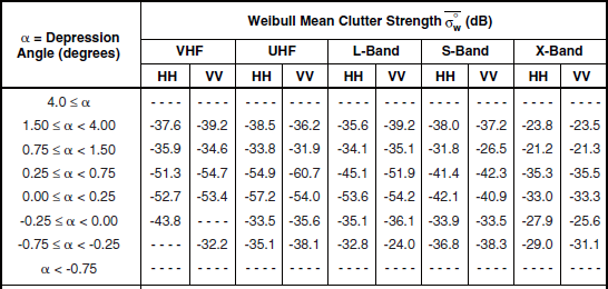
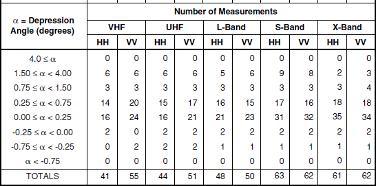
aTable 5.47 defines the population of terrain patches upon which these data are based.
TABLE 5.49
Numbers of Terrain Patches and Measured Clutter Histograms for Mountain Terrain, by Depression Anglea,b,c
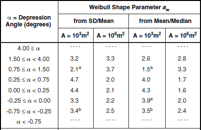
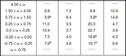
* Table 5.47 defines the population of terrain patches and measurements upon which these data are based.
aFootnoted values apply at A = 104 m2, not 103 m2.
bFootnoted values apply at A = 105 m2, not 103 m2.
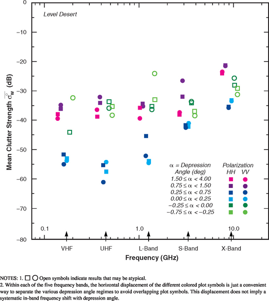
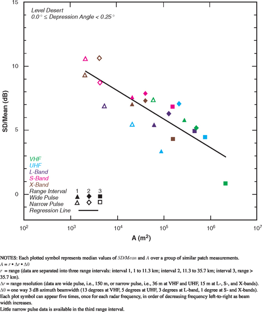
FIGURE 5.43 Ratio of standard deviation-to-mean (SD/Mean) vs radar spatial resolution A for level desert with depression angle between 0.0 and 0.25 degrees.
The low angle (cyan, dark blue) level desert mean clutter strength results in Figure 5.42 for the most part come from Knolls. In contrast, the high angle (purple, magenta) level desert mean clutter strength results in Figure 5.42 for the most part come from Booker Mountain. The high angle level desert results are very similar to the high angle low-relief desert results of Figure 5.40. The high angle level desert results also show the very remarkable ∼15 dB increase in mean clutter strength from S-band to X-band at high angles and from low angle to high angle at X-band previously described in the low-relief desert results of Figure 5.40.
Modeling information for spreads in clutter amplitude distributions from level desert is given in Table 5.49 and Figure 5.43. A strong trend is shown of decreasing spread with increasing cell size. A weaker trend is shown of decreasing spread with increasing depression angle. The scatter plot of Figure 5.43 shows relatively tight correlation about the regression line. This plot is very similar to that of low-relief desert in Figure 5.41.
5.4.8 MOUNTAINOUS TERRAIN
As with desert terrain, mountain terrain does not overtly appear in the terrain classification systems employed herein (see Tables 2.1 and 2.2). A criterion utilized to specify mountain clutter within the Phase One measurement database is that the mountain clutter must come from two Phase One sites—viz., Plateau Mountain and Waterton—that were situated in what is obviously extremely mountainous terrain in the Canadian Rocky Mountains. Plateau Mountain was a high site; Waterton was a low site; both sites are further described in Sections 2.4.2.1 and 3.4.1.2. Further criteria for a clutter patch to be accepted as mountainous at either of these two sites are that its landform classification must be ridged, moderately steep, or steep (see Table 2.2); and its land cover classification must be barren (e.g., perennial-snow-and-ice), rangeland, or forest (see Table 2.1). Table 5.50 indicates that, for mountain terrain thusly defined, there are available 1,653 measured Phase One clutter amplitude distributions from 133 clutter patches for which the terrain within the patch meets these criteria for being mountainous.
TABLE 5.50
Numbers of Terrain Patches and Measured Clutter Histograms for Mountain Terrain, by Depression Anglea,b,c
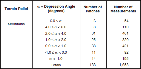
aCanadian Rocky Mountain terrain. Waterton and Plateau Mountain sites. Predominantly barren or forested land cover. Mountain terrain does not include long-range mountain terrain.
bA terrain patch is a land surface macroregion usually several kms on a side (median patch area = 12.62 km2).
cA measured clutter histogram contains all of the temporal (pulse by pulse) and spatial (resolution cell by resolution cell) clutter samples obtained in a given measurement of a terrain patch. A terrain patch was usually measured many times (nominally 20) as RF frequency (5), polarization (2), and range resolution (2) were varied over the Phase One radar parameter matrix.
Clutter modeling information for mountains is given in Tables 5.51 and 5.52 and Figures 5.44 and 5.45. In Figure 5.44, mean clutter strengths for mountains are seen to be very strong, and, like high-relief forest (Figure 5.24), to show a significant trend of decreasing clutter strength with increasing frequency VHF to X-band (compare with the repeat sector mountain data of Figure 3.21; see also Figure 3.2). This trend in mountain terrain is due to increasing absorption of RF power from the incident radar wave by tree foliage with increasing frequency as discussed in Chapter 3, Section 3.4.1.2. As discussed there, when the mountain slopes are not forested, this trend disappears. Also, as in high-relief forest (Figure 5.24), there are significant trends with depression angle in most bands in the mountain data of Figure 5.44, but the trends are more complicated than those of increasing strength with increasing angle exhibited in forest. In fact, there is an inverse trend of decreasing strength with increasing angle in the mountain data of Figure 5.44 similar to the inverse trend shown in the high-relief desert data of Figure 5.38, which exists for the same reason in the mountain data as previously explained for the high-relief desert data. However, in the lower three bands in the mountain data of Figure 5.44 where depression angle effects are significant, the inverse trend is from the 1° to 2° depression angle regime (dark blue) through 2° to 4° (purple) to 4° to 6° (magenta) and > 6° (red); the trend does not include the 0° to 1° (cyan) data. In fact, looking closely at the mountain data in the lower three bands in Figure 5.44, an opposite, more common trend of increasing strength with increasing angle is seen from the −1° to 0° depression angle regime (dark green) to 0° to 1° (cyan) to 1° to 2° (dark blue). So the strongest mountain clutter occurs in all three lower bands in the 1° to 2° depression angle regime (dark blue), with mean strengths decreasing both with increasing depression angle (lower terrain) and decreasing depression angle (higher terrain) from there.
TABLE 5.51
Mean Clutter Strength ![]() and Number of Measurements for Mountain Terrain, by Frequency Band, Polarization, and Depression Anglea
and Number of Measurements for Mountain Terrain, by Frequency Band, Polarization, and Depression Anglea
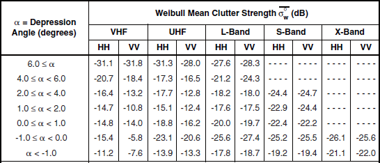
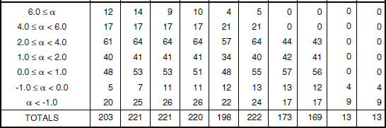
aTable 5.50 defines the population of terrain patches upon which these data are based.
TABLE 5.52
Shape Parameter aw and Ratios of Standard Deviation-to-Mean (SD/Mean) and Mean-to-Median for Mountain Terrain, by Spatial Resolution A and Depression Angle*
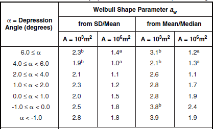
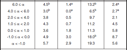
aFootnoted values apply at A = 105 m2, not 106 m2.
bFootnoted values apply at A = 104 m2, not 103 m2.
*Table 5.50 defines the population of terrain patches and measurements upon which these data are based.
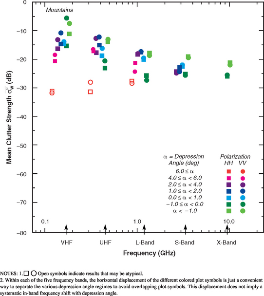
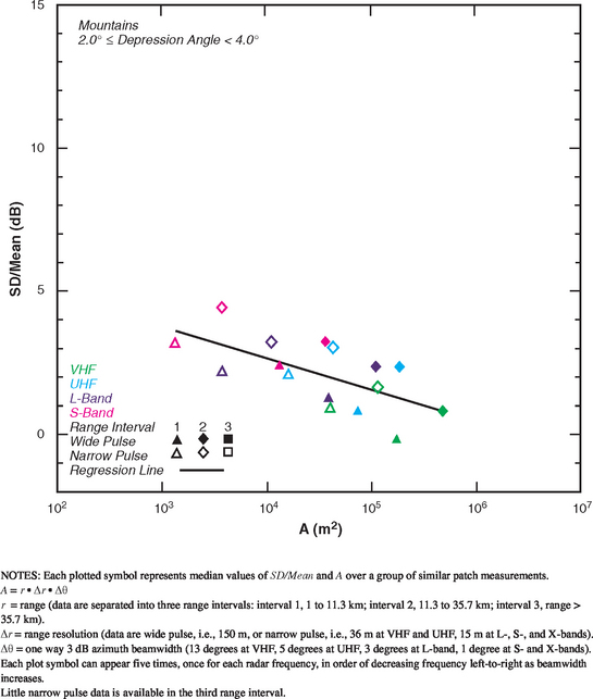
FIGURE 5.45 Ratio of standard deviation-to-mean (SD/Mean) vs radar spatial resolution A for mountain terrain with depression angle between 2.0 and 4.0 degrees.
Modeling information for spreads in clutter amplitude distributions from mountain terrain is given in Table 5.52 and Figure 5.45. Spreads in mountain clutter amplitude distributions are small (although generally still significantly wider than Rayleigh statistics)—in fact, spreads in mountain clutter are the least of any terrain type (high-relief forest has the next lowest spread). In particular, the mountain spreads for large A (A ≅ 106 m2) are nearer unity (i.e., more approaching Rayleigh) in Table 5.52 than any other terrain type (compare with high-relief forest, Table 5.26). These low spreads in mountain clutter amplitude distributions are due to the high terrain slopes and corresponding full illumination of the mountain clutter patches. As with most other terrain types, there exists a significant trend of decreasing spread with increasing cell size A in the mountain data of Table 5.52 and Figure 5.45.
5.4.8.1 LONG-RANGE MOUNTAINS
When strong clutter from visible terrain at long range occurs in surface-sited radars, it usually comes from mountains because only mountains are high enough to be visible at long range over the spherical earth. Long-range mountain clutter is discussed at some length in Chapter 3, Appendix 3.B, Section 3.B.3. The long-range mountain clutter data discussed in Chapter 3 were measured over broad azimuth sectors from the Canadian Rocky mountains at three Alberta sites. In what follows, long-range mountain clutter data are presented, also from the Canadian Rocky mountains, but as measured within clutter patches as selected from six Alberta measurement sites. Table 5.53 indicates that there are available 721 measured Phase One clutter amplitude distributions from 80 long-range mountain clutter patches at these six sites. These long-range mountain clutter patches were predominantly of barren or perennial-snow-and-ice land cover classification, with some secondary occurrences of forest. Ranges to these 80 patches varied from 45 to 143 km. As shown in Table 5.53, all 80 long-range mountain clutter patches were observed in a narrow negative depression angle regime, from −0.75° to −1.6°.
TABLE 5.53
Numbers of Terrain Patches and Measured Clutter Histograms for Long-Range Mountain Terrain, by Depression Anglea,b,c
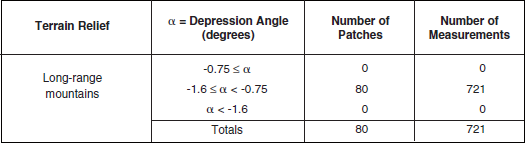
aRanges from 45 to 143 kilometers. Canadian Rocky Mountain terrain. Six sites. Predominantly barren or forested land cover. Long-range mountain terrain is not included within mountain terrain.
bA terrain patch is a land surface macroregion usually several kms on a side (median patch area = 12.62 km2).
cA measured clutter histogram contains all of the temporal (pulse by pulse) and spatial (resolution cell by resolution cell) clutter samples obtained in a given measurement of a terrain patch. A terrain patch was usually measured many times (nominally 20) as RF frequency (5), polarization (2), and range resolution (2) were varied over the Phase One radar parameter matrix.
Mean clutter strengths for long-range mountains are given in Table 5.54 and plotted in Figure 5.46. Mean clutter strengths for long-range mountains are strong, but not as strong as mountains at closer ranges (compare with Figure 5.44), particularly in the lower bands. A gentle trend of decreasing clutter strength with increasing frequency, VHF to S-band, is observed in Figure 5.46, with X-band increasing slightly over S-band. These results may be compared with the generally weaker long-range mountain clutter as reduced over very large azimuth sectors shown in Figure 3.B.10 of Appendix 3.B—these latter data are weaker because they are not patch-specific but instead incorporate significant amounts of macroshadow, particularly at the higher radar frequencies. The long-range mountain clutter of Figure 5.46 is weaker than mountain clutter at shorter ranges (Figure 5.44), particularly in the lower bands, because of propagation losses over the long ranges at near grazing incidence.
TABLE 5.54
Mean Clutter Strength ![]() and Number of Measurements for Long-Range Mountain Terrain, by Frequency Band, Polarization, and Depression Anglea
and Number of Measurements for Long-Range Mountain Terrain, by Frequency Band, Polarization, and Depression Anglea
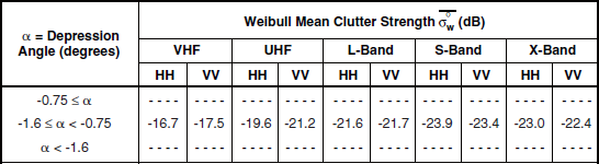
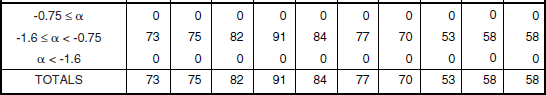
aTable 5.53 defines the population of terrain patches upon which these data are based.
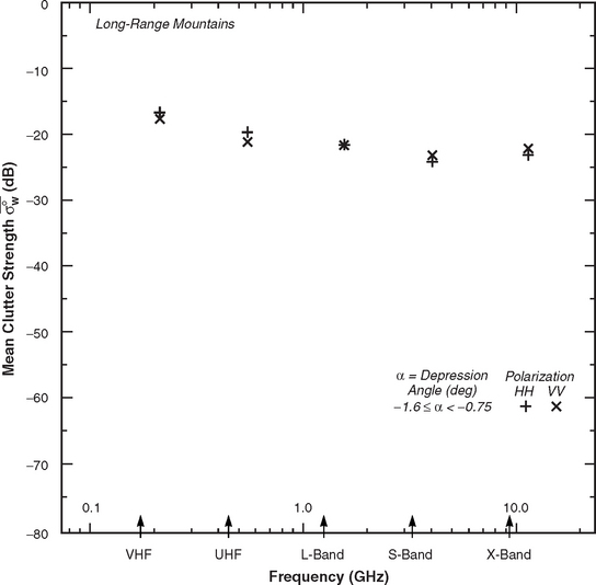
Modeling information for spreads in clutter amplitude distributions from long-range mountains is given in Table 5.55 and Figure 5.47. Cell area A is very large in all these long-range data. However, over the range of large cell areas available, there remains a significant trend of decreasing spread with increasing cell size.
TABLE 5.55
Shape Parameter aw and Ratios of Standard Deviation-to-Mean (SD/Mean) and Mean-to-Median for Long-Range Mountain Terrain, by Spatial Resolution A and Depression Angle*
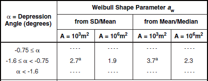
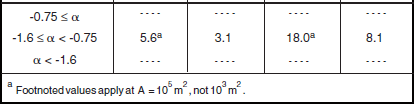
aFootnoted values apply at A = 105 m2, not 103 m2.
*Table 5.53 defines the population of terrain patches and measurements upon which these data are based.
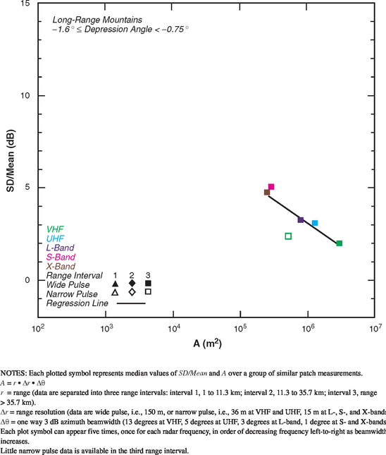
5.5 PPI CLUTTER MAP PREDICTION
Of particular interest is the site-specific prediction of plan-position indicator (PPI) land clutter maps for ground-sited radars. Such prediction involves simulating the spatial variation of land clutter. As previously discussed, first DTED is used to establish geometric line-of-sight terrain visibility from the radar antenna position, then the strength of the clutter in each visible cell is provided as a random realization from a Weibull distribution for which the coefficients ![]() and aw are appropriately selected from the tables provided in Sections 5.3 or 5.4.
and aw are appropriately selected from the tables provided in Sections 5.3 or 5.4.
An example of this procedure for predicting a PPI clutter map is shown in Figure 5.48. This figure compares modeled and measured clutter maps for an X-band radar of horizontal polarization and 150-m range resolution situated at Brazeau, a forested wilderness site in Alberta, Canada at latitude 53.04° N and longitude 115.43° W (see Chapter 3). The maximum range of the clutter maps in Figure 5.48 is 24 km; the clutter map measured by the Phase One radar is to the left, the simulated map is to the right. The black regions in the simulated map are masked terrain regions as predicted using DTED. They correspond reasonably well with black regions in the measured map where the radar is at or close to its noise floor. As the quality of available DTED continues to improve, so does the fidelity of prediction of the black masked regions in such maps. Within the visible colored regions in the modeled map of Figure 5.48, there is generally good agreement with measurement in the general range of colors predicted in any particular region, although the cell-to-cell spatial correlation in the measured map is not precisely followed in the modeled map.
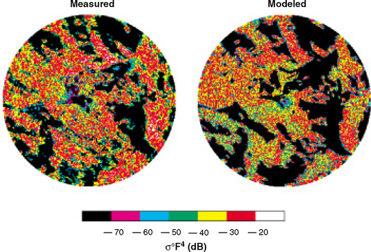
FIGURE 5.48 Comparison of measured and modeled PPI ground clutter maps at Brazeau, Alta. Maximum range = 24 km. X-band, 150-m range resolution, horizontal polarization.
The validity of such predictions is not based on subjective judgment of how good a modeled clutter map appears, or even on how closely modeled and measured cumulative σ° distributions compare within regions or over whole sites. Rather the validity of such predictions is based in the final analysis on how closely a particular radar system performance measure computed using modeled clutter compares to the corresponding performance measure computed using measured clutter. When tested in this manner, the Weibull statistical clutter models generally perform with highly satisfactory accuracy in computing clutter-limited system performance.
5.5.1 MODEL VALIDATION
The Weibull clutter model has been in use at Lincoln Laboratory for a number of years in radar system studies involving clutter-limited operation against various airborne targets. These studies have involved radar systems ranging in frequency from VHF to X-band. Since the clutter model directly affects the outcomes of such studies, strong and ongoing interest exists in validating and improving the clutter model. In validating a clutter model, a radar engagement with a target is hypothesized to take place at one of the Phase One clutter measurement sites, and system performance is computed in two ways: (1) using the actual measured clutter at that site, and (2) using the clutter model to simulate clutter at that site. Successful validation requires that the performance measure computed using modeled clutter be acceptably similar to that computed using the actual clutter. Model validation encompasses many measurement sites.
For X-band tracking systems, the Weibull model generally works well in predicting the performance parameters employed in such studies. System performance is then generalized by computing the median performance parameter of the system over many sites. A simple spherical earth, constant-σ° clutter model cannot deliver the same general performance as the more in-depth Weibull model. That is, the constant σ° required in the simple model is system and performance-parameter dependent, whereas the Weibull statistical model is adaptive and resilient enough to work well for any clutter-limited system or performance parameter.
For VHF surveillance systems, radar performance parameters can be more difficult to predict due to propagation effects. The Weibull VHF model remains accurate in terrain of significant relief where propagation effects are not severe. However, in level open terrain, the accuracy of the Weibull model can, in some circumstances, be improved by adding deterministic computations of multipath propagation.
5.5.2 MODEL IMPROVEMENT
The clutter modeling information of Chapter 5 represents low-angle land clutter as a Weibull statistical process occurring over visible terrain regions. The Weibull distributions aggregate the widely varying returns received predominantly from an infinitude of spatially localized discrete sources. Studies have been conducted to shed further light on higher-order parametric effects that occur in low-angle land clutter beyond the level at which clutter modeling information is provided in Chapter 5. These studies include the following:
1. separating the strongest discretes and introducing grazing angle dependence on the residual clutter background (see Appendix 4.D);
2. introducing clutter into shadowed regions (see Appendix 4.D);
3. utilizing improved cell-specific land cover information (e.g., Landsat data, see Section 4.4.1);
4. improving propagation prediction (e.g., SEKE; Parabolic Equation techniques; Method of Moments techniques) at clutter source heights (see Section 1.5.4 and Appendix 3.B);
5. investigating non-site-specific clutter modeling approaches which incorporate spatial patchiness on the basis of mathematically derived stochastic processes as opposed to deterministic site-specific visibility in DTED (see Sections 1.4.2 and 4.3.3.1).
As indicated, each of these subjects has been mentioned or discussed elsewhere in this book.
Figure 4.3 (in Chapter 4) conveniently represents the structure of the Weibull statistical clutter model. Within this structure, what actually exists is an adaptive computer-resident modeling capability. That is, 59,804 measured clutter spatial amplitude distributions exist as computer files together with their terrain descriptive parameters. The clutter model is the template by which these data are sorted. Not only can general templates be provided for general terrain types such as are given in Sections 5.3 and 5.4, but also the template can be adjusted to provide more detailed results for terrain types highly specific to an individual user’s particular interests.
5.6 SUMMARY
Chapter 5 provides land clutter modeling information for surface radar on the basis of extensive Phase One five-frequency 360° survey clutter measurements at 42 different sites of widely varying terrain type (see Chapter 3). The modeling information provided specifies the probability distribution encompassing the spatial cell-to-cell variability of clutter amplitudes for a given set of parametric conditions. Important parameters are of three types: (1) those of the radar—frequency, resolution, polarization; (2) the angle of illumination of the terrain—that is, the depression angle below the horizontal at which the radar views the terrain; and (3) parameters descriptive of the terrain—its relief and land cover.
The probability distributions are specified in terms of Weibull statistics. A modeling approach is followed, as developed in earlier chapters of this book, in which radar spatial resolution affects only the shape parameter aw of the Weibull distribution, and radar frequency affects only the mean of the distribution ![]() . This decoupling of the effects of resolution and frequency on the modeled clutter distributions is central to the success of this approach to clutter modeling. The fact that aw depends only on radar resolution and not radar frequency means that results from the various Phase One radar frequency bands and corresponding widely varying azimuth beamwidths are able to be combined to generalize effects with spatial resolution across a wide range of resolutions. The fact that the mean strength
. This decoupling of the effects of resolution and frequency on the modeled clutter distributions is central to the success of this approach to clutter modeling. The fact that aw depends only on radar resolution and not radar frequency means that results from the various Phase One radar frequency bands and corresponding widely varying azimuth beamwidths are able to be combined to generalize effects with spatial resolution across a wide range of resolutions. The fact that the mean strength ![]() depends only on radar frequency and not resolution (
depends only on radar frequency and not resolution (![]() is the only resolution-invariant attribute of the clutter amplitude distribution) reduces the dimensionality of the modeling construct and allows fundamental trends in
is the only resolution-invariant attribute of the clutter amplitude distribution) reduces the dimensionality of the modeling construct and allows fundamental trends in ![]() to emerge. Both
to emerge. Both ![]() and aw are dependent on depression angle and terrain type.
and aw are dependent on depression angle and terrain type.
In contrast to the much simpler interim clutter model presented in Chapter 4 (which was of the same modeling structure as the information presented in Chapter 5), the information in Chapter 5 is presented without any smoothing or extrapolation as was necessary in the interim model. The number of measurements underlying each value of ![]() and aw in Chapter 5 is also provided as a first assessment of generality. Occasionally, open plot symbols are used in the mean strength figures of Chapter 5 to indicate lightly-sampled
and aw in Chapter 5 is also provided as a first assessment of generality. Occasionally, open plot symbols are used in the mean strength figures of Chapter 5 to indicate lightly-sampled ![]() values that appear to be non-general.
values that appear to be non-general.
Clutter modeling information is provided in Chapter 5 for both general rural terrain and for a number of specific terrain types. In general rural terrain, consistent general trends emerge of increasing mean clutter strength ![]() with increasing depression angle, in all five frequency bands and for both high- and low-relief terrain. The reason these trends emerge so consistently in the general rural terrain results of Chapter 5 is that each plotted point is typically based on hundreds of measurements, among which there is much individual variability. Concerning radar frequency dependence in general rural terrain, at high depression angles mean clutter strength decreases with increasing radar carrier frequency as ∼(1/f); at low depression angles mean strength increases with increasing carrier frequency as ∼f; there is no single simple frequency dependence in low-angle land clutter. Mean strengths at HH-polarization are usually 1 or 2 dB weaker than at VV-polarization (a full matrix of information is available at both polarizations). Mean clutter strength rises rapidly with increasing negative depression angle (i.e., terrain observed at higher elevations than the radar). A large amount of generalized clutter modeling information is presented in Chapter 5 for general rural terrain. These results are among the more important of the Phase One findings. They show consistent general trends, especially with depression angle, but also with terrain relief and radar frequency, to sort out a phenomenon of which the most salient characteristic is variability.
with increasing depression angle, in all five frequency bands and for both high- and low-relief terrain. The reason these trends emerge so consistently in the general rural terrain results of Chapter 5 is that each plotted point is typically based on hundreds of measurements, among which there is much individual variability. Concerning radar frequency dependence in general rural terrain, at high depression angles mean clutter strength decreases with increasing radar carrier frequency as ∼(1/f); at low depression angles mean strength increases with increasing carrier frequency as ∼f; there is no single simple frequency dependence in low-angle land clutter. Mean strengths at HH-polarization are usually 1 or 2 dB weaker than at VV-polarization (a full matrix of information is available at both polarizations). Mean clutter strength rises rapidly with increasing negative depression angle (i.e., terrain observed at higher elevations than the radar). A large amount of generalized clutter modeling information is presented in Chapter 5 for general rural terrain. These results are among the more important of the Phase One findings. They show consistent general trends, especially with depression angle, but also with terrain relief and radar frequency, to sort out a phenomenon of which the most salient characteristic is variability.
Chapter 5 also provides generalized clutter modeling information for eight specific terrain types—urban, farmland, forest, shrubland, grassland, wetland, desert, and mountains. As expected, these results show that clutter is strong in urban and mountain terrain, and weaker in desert and wetland terrain. In urban terrain at high depression angle, mean clutter strength ![]() is relatively frequency invariant in the −15 to −20 dB range. Mountain clutter shows a trend of decreasing strength with increasing radar frequency, so that it is stronger than urban clutter at VHF and UHF, weaker at S- and X-bands. Mountain clutter also shows a countertrend of decreasing strength with increasing depression angle—looking broadside at high peaks causes stronger clutter than looking down at lower peaks. Desert clutter at high depression angles is approximately frequency invariant VHF to S-band (at
is relatively frequency invariant in the −15 to −20 dB range. Mountain clutter shows a trend of decreasing strength with increasing radar frequency, so that it is stronger than urban clutter at VHF and UHF, weaker at S- and X-bands. Mountain clutter also shows a countertrend of decreasing strength with increasing depression angle—looking broadside at high peaks causes stronger clutter than looking down at lower peaks. Desert clutter at high depression angles is approximately frequency invariant VHF to S-band (at ![]() dB), but increases dramatically by ∼15 dB (to
dB), but increases dramatically by ∼15 dB (to ![]() dB) at X-band. At low angles, desert clutter is much weaker, but level desert at low angles (with
dB) at X-band. At low angles, desert clutter is much weaker, but level desert at low angles (with ![]() to −60 dB in the lower bands) is not as weak as wetland at low angles (with
to −60 dB in the lower bands) is not as weak as wetland at low angles (with ![]() to −70 dB in the lower bands). Both level desert and wetland clutter at low angles show intrinsic σ° (aside from multipath losses) to be significantly stronger at VHF (170 MHz) than UHF (430 MHz). Many other general effects may be seen in the clutter modeling information for mean clutter strengths provided for specific terrain types in Chapter 5. In total there is 70 dB of variability in mean clutter strength between the strongest and weakest measurements of land clutter. However, specification of terrain type, terrain relief, and the depression angle at which the terrain is illuminated allows the mean clutter strength from that terrain to be accurately predicted, even over such a wide range. It is evident that non-terrain-specific approaches to land clutter modeling must inherently involve large uncertainties.
to −70 dB in the lower bands). Both level desert and wetland clutter at low angles show intrinsic σ° (aside from multipath losses) to be significantly stronger at VHF (170 MHz) than UHF (430 MHz). Many other general effects may be seen in the clutter modeling information for mean clutter strengths provided for specific terrain types in Chapter 5. In total there is 70 dB of variability in mean clutter strength between the strongest and weakest measurements of land clutter. However, specification of terrain type, terrain relief, and the depression angle at which the terrain is illuminated allows the mean clutter strength from that terrain to be accurately predicted, even over such a wide range. It is evident that non-terrain-specific approaches to land clutter modeling must inherently involve large uncertainties.
In addition to mean clutter strength ![]() , the land clutter modeling information of Chapter 5 also specifies the shapes aw of clutter amplitude distributions. As mentioned, the shape or spread of the distribution is fundamentally dependent on the spatial resolution of the radar. The modeling information of Chapter 5 shows that for almost all terrain, there exists a strong trend of decreasing spread (decreasing aw) with increasing area A of the radar resolution cell. Spreads in forested terrain—including forested mountain terrain—are much less than spreads in open terrain for given values of cell size A, although both forested and open terrain show the strong trends of decreasing aw with increasing A. Values of aw are generally specified over the range from A = 103 m2 to A = 106 m2. Many of the results appear to indicate that the extremely widely spread Weibull distributions (e.g., aw = 5) that exist for small cell sizes rapidly diminish in spread with increasing A and appear to be approximately approaching Rayleigh statistics (aw = 1) for very large cells (e.g., A = 107 or 108 m2) beyond the available range of the data. However, what occurs for larger cell sizes (A > 106 m2) or smaller SAR-like cell sizes (A < 103 m2) is unknown—there are physical reasons to expect that the linear trends observed of aw vs log A should not extrapolate to very small cell sizes. In addition to the strong trend of decreasing spread with increasing cell size, there also often exist suggestions of a weaker trend of decreasing spread with increasing depression angle particularly for smaller cell sizes.
, the land clutter modeling information of Chapter 5 also specifies the shapes aw of clutter amplitude distributions. As mentioned, the shape or spread of the distribution is fundamentally dependent on the spatial resolution of the radar. The modeling information of Chapter 5 shows that for almost all terrain, there exists a strong trend of decreasing spread (decreasing aw) with increasing area A of the radar resolution cell. Spreads in forested terrain—including forested mountain terrain—are much less than spreads in open terrain for given values of cell size A, although both forested and open terrain show the strong trends of decreasing aw with increasing A. Values of aw are generally specified over the range from A = 103 m2 to A = 106 m2. Many of the results appear to indicate that the extremely widely spread Weibull distributions (e.g., aw = 5) that exist for small cell sizes rapidly diminish in spread with increasing A and appear to be approximately approaching Rayleigh statistics (aw = 1) for very large cells (e.g., A = 107 or 108 m2) beyond the available range of the data. However, what occurs for larger cell sizes (A > 106 m2) or smaller SAR-like cell sizes (A < 103 m2) is unknown—there are physical reasons to expect that the linear trends observed of aw vs log A should not extrapolate to very small cell sizes. In addition to the strong trend of decreasing spread with increasing cell size, there also often exist suggestions of a weaker trend of decreasing spread with increasing depression angle particularly for smaller cell sizes.
In totality, the clutter modeling information of Chapter 5 provides a condensed and unified, general codification of the properties of low-angle land clutter. Historically, there has been little indication of connectivity or unity among the many measurements reported by many different investigators. The main reason that has allowed Chapter 5 to successfully generalize low-angle land clutter is the large amounts of measurement data involved. Averaging over (medianizing) large amounts of data has allowed fundamental trends to emerge that are often obscured by specific effects in individual measurements.
Appendix 5.A WEIBULL STATISTICS
5.A.1 introduction
Chapter 5 provides empirical modeling information for low-angle radar land clutter spatial amplitude statistics in terms of Weibull probability distributions [1]. The purpose of this appendix is to provide information indicating why Weibull distributions were selected to model low-angle clutter in Chapter 5 and elsewhere in this book, as opposed to other possible distribution functions, including in particular the lognormal distribution and the K-distribution. The reasons for using Weibull distributions are as follows:
1. The Weibull distribution is a simple two-parameter distribution that can accommodate the extreme spreads that occur in low-angle clutter spatial amplitude statistics.
2. The Weibull distribution generally (but not without occasional exception) fits the measured low-angle distributions better than other candidate distributions that can also accommodate wide spread, including the lognormal and K-distributions.
3. The Weibull distribution is analytically simple and tractable, more so than the lognormal or K-distributions.
4. A Weibull distribution of clutter power (as used here in representing clutter strength σ°F4) of shape parameter aw remains a Weibull distribution when transformed to clutter voltage, of shape parameter aw/2.
5. The Weibull distribution provides decreasing spread with decreasing values of shape parameter aw and in the limiting case degenerates to an exponential distribution [exponential for clutter power = σ°; Rayleigh for clutter voltage = (σ°)1/2]. This mimics the behavior of measured clutter amplitude distributions which, with increasing depression angle and cell size, also show decreasing spread and, in the limiting high-angle case for surface radar (viz., 8° or so), also often degenerate to approximately Rayleigh distributions (e.g., see Table 2.B.1).
This appendix covers the following material. Section 5.A.2 further describes Weibull distributions. A number of plots are provided which give added insight into the behavior of Weibull distributions, and which make the clutter modeling information of Chapter 5—given in terms of Weibull coefficients—easier to work with. Section 5.A.3 numerically examines the shapes of the cumulative distribution function (cdf) of theoretical Weibull distributions as plotted against nonlinear Weibull and lognormal probability ordinates, and compares them with lognormal and K-distribution shapes plotted against the same ordinates. This provides understanding on how to interpret upwards and downwards curvature in cdf shapes of measured spatial clutter amplitude distributions when plotted against these ordinates, as to whether they are tending towards Weibull, lognormal, or K-shapes. Examination of the shapes in the extreme high tails is also included. Section 5.A.4 illustrates how Weibull distributions often fit measured low-angle clutter amplitude distributions better than other analytic distributions by comparing fits obtained with
Weibull, lognormal, and K-distributions to some measured Phase One X-band farmland clutter data.
5.A.2 WEIBULL DISTRIBUTIONS; aw= 1, 2, 3, 4, 5
The Weibull probability density function (pdf) may be written
In Eq. (5.A.1), as elsewhere in this book, the random variable x represents clutter strength σ°F4, where F is the pattern propagation factor [2]. The quantity x = σ°F4 is in some places abbreviated as σ° in this appendix. Also, as represented elsewhere in this book, the Weibull shape parameter aw is related to b in Eq. (5.A.1) as
The scale parameter c in Eq. (5.A.1) is related to the median value of clutter strength x50 (or σ°50) as
[cf. Eq. (2.B.18)]. The Weibull cumulative distribution function (cdf) follows from Eq. (5.A.1), as
The ratio of variance to the square of the mean for a Weibull distribution is given by
where Γ is the Gamma function, ![]() is the mean of x, and var(x) is the variance of x. The ratio of standard deviation-to-mean in a Weibull distribution, i.e.,
is the mean of x, and var(x) is the variance of x. The ratio of standard deviation-to-mean in a Weibull distribution, i.e., ![]() , which is much used in Chapter 5, is
, which is much used in Chapter 5, is
The ratio of mean-to-median in a Weibull distribution is given by
Definitions, relationships, and other matters involving the Weibull distribution are also discussed in Appendix 2.B.
Figure 5.A.1 plots the shape of the Weibull pdf as given by Eq. (5.A.1) for four values of shape parameter aw—namely, aw = 0.666, 0.5, 1, and 2, following Sekine and Mao [1]. Table 5.A.1 shows the aw shape regimes of Weibull distributions. It is apparent in Figure 5.A.1 that, for aw < 1, the shapes are peaked at a positive modal value of x [for the Weibull distribution of Eq. (5.A.1), mode ![]() ], and the pdf decays from its modal peak to zero at both x = 0 and x = ∞. In contrast, for aw >> 1, the shapes are not peaked.
], and the pdf decays from its modal peak to zero at both x = 0 and x = ∞. In contrast, for aw >> 1, the shapes are not peaked.
TABLE 5.A.1
Shape Regimes of Weibull Distribution
| aw | Shape |
| < 1 | Peaked |
| = 1 | Negative Exponential |
| > 1 | Subexponential |
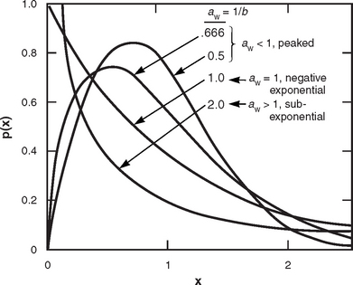
FIGURE 5.A.1 Weibull pdf p(x) ≡ bxb−1 e−xb. Here x50 = (ln 2)aw, so c = 1. (After Sekine and Mao [1]; by permission, © 1990 IEE.)
For aw = 1, the pdf is a negative exponential and decays from its maximum value of unity at x = 0 to reach zero at x = ∞. For aw >1, the shapes are like the negative exponential in that they also decay from maximum values at x = 0 to reach zero at x = ∞. These shapes for aw > 1 are called subexponential because their exponents b = 1/aw are less than unity. Although similar to the negative exponential shape for aw = 1, the subexponential shapes for aw > 1 decay with increasing x from maximum values at x = 0 greater than unity, first at rates faster than the negative exponential, and then for large values of x at rates slower than the negative exponential. It is these slow rates of decay and long tails for large values of x that are of interest here in that they mirror the behavior of low-angle land clutter spatial amplitude distributions.
Thus interest is in the subexponential Weibull pdf’s for which aw >1. Note that for simplicity, Figure 5.A.1 is plotted for c = 1 which means for ![]() —see Eqs. (5.A.1) and (5.A.3). This is done in the interest of making a simple plot, but the plot is not representative of realistic clutter amplitudes. In a number of results to follow in Sections 5.A.2 and 5.A.3, this appendix sets x50 = 0.0001 (i.e., median clutter strength = −40 dB) and lets the Weibull shape parameter range subexponentially over the five values aw = 1, 2, 3, 4, 5. These values of x50 and aw are representative of the values occurring for these parameters in many of the actual measured clutter spatial amplitude distributions shown in the main body of Chapter 5 and elsewhere in this book.
—see Eqs. (5.A.1) and (5.A.3). This is done in the interest of making a simple plot, but the plot is not representative of realistic clutter amplitudes. In a number of results to follow in Sections 5.A.2 and 5.A.3, this appendix sets x50 = 0.0001 (i.e., median clutter strength = −40 dB) and lets the Weibull shape parameter range subexponentially over the five values aw = 1, 2, 3, 4, 5. These values of x50 and aw are representative of the values occurring for these parameters in many of the actual measured clutter spatial amplitude distributions shown in the main body of Chapter 5 and elsewhere in this book.
Thus Figure 5.A.2 plots the shape of the Weibull pdf as given by Eq. (5.A.1) for Weibull parameters x50 = 0.0001 and aw = 1, 2, 3, 4, 5. To accommodate these realistic parameters, logarithmic scales are used for both abscissa and ordinate (i.e., log-log paper). The median value x50 = 0.0001 is shown at the extreme left end of the abscissa. Long decaying tails are seen over increasing values of x from the median value, of increasing length and decreasing rate of decay with increasing aw. The label “Gaussian” on the aw = 1 curve means that the in-phase (I) and quadrature (Q) clutter voltage components are each of zero-mean equal-variance Gaussian shape, which implies that the amplitude of the clutter voltage [I2 + Q2]1/2 is Rayleigh distributed, and the clutter power σ° = I2 + Q2 is exponentially distributed.
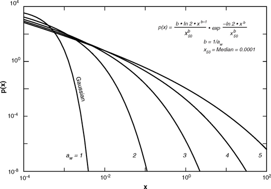
The distributions of Figure 5.A.2 are not similar to these actually observed or plotted in this book, when histograms of measured clutter spatial amplitude statistics are formed. The reason is that the clutter histograms as shown herein are formed of decibel values of clutter strength to keep them manageable because of the wide ranges of clutter power that are involved. Thus the histograms are formed in bins of width specified in decibels, typically in bins 1 dB wide (see Appendix 2.B). This constitutes a logarithmic transformation y = 10log10x. Figure 5.A.3 shows the logarithmically transformed Weibull pdf of Eq. (5.A.1) such that p(x)dx = p(y)dy. Like Figure 5.A.2, Figure 5.A.3 continues to show results for x50 = 0.0001 and aw = 1, 2, 3, 4, 5. The pdf shapes in Figure 5.A.3 look like the typical shapes of the measured clutter histograms, examples of which are shown in a number of places in this book. These pdf shapes show a long, slowly diminishing, high-side tail of increasing extent and decreasing rate of decay with increasing value of aw, which mimics the behavior of the measured histograms. All five pdf’s in Figure 5.A.3 are of bell shape, between narrow and high (aw = 1) and wide and low (aw = 5). The median value of 10log10x50 = y50 = −40 dB is evident near the peaks of the bell shapes. Many of the measured histograms do not show much or any of the diminishing shape for low values of y to the left because the histograms become noise-limited for low values of y.
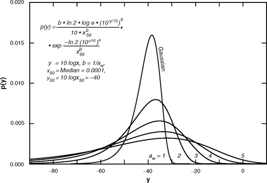
FIGURE 5.A.3 The logarithmically transformed Weibull probability density function p(y); y50 = −40; aw = 1, … 5.
Figure 2.28 in Chapter 2 plots the shape of the Weibull cdf as given by Eq. (5.A.4) against a Weibull ordinate, also for x50 = σ°50 = 0.0001 and aw = 1, 2, 3, 4, 5. The increasing extent of the high-side tail with increasing values of aw is evident in Figure 2.28, as are the increasingly strong values of mean clutter strength in these distributions as a result of the high-side tails, and the increasingly large values of mean/median ratio with increasing aw.
Figure 5.A.4 shows plots of the ratio of standard deviation-to-mean ![]() vs aw, and of the ratio of mean-to-median
vs aw, and of the ratio of mean-to-median ![]() vs aw, as given by Eqs. (5.A.6) and (5.A.7), respectively. Note that these relationships are transcendental, involving the Gamma function. The plots are shown over the range 0 ≤ αw ≤ 6, although principal interest here is in the subexponential range aw > 1. It is apparent that both measures of Weibull spread in Figure 5.A.4—sd/mean and mean/median—increase very rapidly with increasing aw; they are shown as decibel quantities in Figure 5.A.4 to accommodate their rapid increase. As indicated in Figure 5.A.4, when aw = 1 the Weibull distribution degenerates to a simple negative exponential distribution for clutter power and power-like quantities including σ°, which means the in-phase and quadrature components of clutter voltage are distributed as zero-mean equal-variance Gaussians.
vs aw, as given by Eqs. (5.A.6) and (5.A.7), respectively. Note that these relationships are transcendental, involving the Gamma function. The plots are shown over the range 0 ≤ αw ≤ 6, although principal interest here is in the subexponential range aw > 1. It is apparent that both measures of Weibull spread in Figure 5.A.4—sd/mean and mean/median—increase very rapidly with increasing aw; they are shown as decibel quantities in Figure 5.A.4 to accommodate their rapid increase. As indicated in Figure 5.A.4, when aw = 1 the Weibull distribution degenerates to a simple negative exponential distribution for clutter power and power-like quantities including σ°, which means the in-phase and quadrature components of clutter voltage are distributed as zero-mean equal-variance Gaussians.
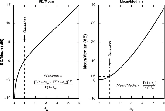
Extensive modeling information for spread in low-angle land clutter distributions is given in Chapter 5 in terms of tabulated and plotted values of both the actual measured quantities of spread in these distributions—namely, ratios of sd/mean and mean/median—and in terms of the modeling parameter used to capture these quantities—namely, the Weibull shape parameter aw. The two plots in Figure 5.A.4 are useful in allowing quick, back-and-forth conversion between these transcendentally-related quantities.
The modeling information for spread in clutter amplitude distributions given in Chapter 5 is given in terms of linear regression between spread values for limiting cell sizes A = 103 m2 and A = 106 m2. The linear regression actually took place in the measured quantities of spread—sd/mean (dB) vs log10A and mean/median (dB) vs log10A. Many examples of the scatter plots of sd/mean (dB) vs log10A and the resulting regression lines are shown in
Chapter 5; similar scatter plots and regression lines were formed of mean/median (dB) vs log10A. The exact use of the modeling information for spread requires linear interpolation on log10A of the provided underlying measured values of spread—sd/mean (dB) or mean/median (dB)—rather than aw directly. However, as shown in the left-hand plot of Figure 5.A.4, the relationship between sd/mean (dB) and aw is essentially linear for values of aw such that aw > 1.5. The value of aw = 1.5 corresponds to a value of sd/mean = 1.90 dB. Almost all values of clutter spread given in Chapter 5 exceed aw = 1.5 and/or sd/mean = 1.90 dB. Since the relationship between sd/mean (dB) and aw is essentially linear for aw > 1.5 and sd/mean > 1.90 dB, it does not matter whether the linear regression is done on aw vs log10A or sd/mean (dB) vs log10A. By contrast, the right-hand plot in Figure 5.A.4 is less linear, so it matters more that, if modeling values of aw are selected as derived from mean/median (dB), in this case the interpolation be of mean/median (dB) vs log10A, not aw vs log10A.
5.A.3 COMPARISON OF WEIBULL, LOGNORMAL, AND K-DISTRIBUTIONS
This section discusses what observed curvature can imply in plots of cdf’s of clutter strength on nonlinear probability scales. The two nonlinear scales of interest are the Weibull scale (if the measured cdf is linear when plotted on a Weibull scale, the measured distribution is Weibull) and the lognormal scale (if the measured cdf is linear when plotted on a lognormal scale, the measured distribution is lognormal). All measured spatial clutter amplitude distributions from clutter patches were plotted on both Weibull and lognormal cumulative probability scales. The derivation of the plot axes in such Weibull and lognormal plots, the plotting of measured clutter distributions in the plots, and the regression analyses to obtain modeling information in the plots are all described in detail in Appendix 2.B. The question of interest here is, what does observed curvature in such plots imply about whether such clutter amplitude distributions are more accurately represented as Weibull, lognormal, or K-distributions?
Figure 5.A.5 is a notional diagram showing the kinds of curvature exhibited by Weibull, lognormal, and K-distributions when plotted as cdf’s using a nonlinear Weibull probability scale as the y-axis. As shown, a Weibull distribution plots as a straight line, a lognormal distribution plots with convex curvature as observed from above (i.e., is downward curving), and a K-distribution plots with concave curvature as observed from above (i.e., is upward curving). The plots of measured clutter cdf’s in overall measure tend more toward linearity on Weibull plots than they tend to be of strong general upwards or strong general downwards curvature, although examples of all three kinds of curvature occur in the data.
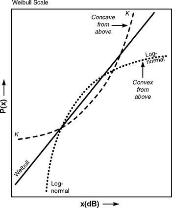
FIGURE 5.A.5 Weibull, lognormal, and K-distribution comparative cdf shapes plotted on a Weibull scale.
The notional diagrams of Figure 5.A.6 expand the discussion of Figure 5.A.5. Part (a) shows a Weibull distribution, which as required plots linearly against the Weibull y-axis used there; part (b) shows the same Weibull distribution which exhibits upward curvature (concave from above) when plotted against the lognormal y-axis used there. A lognormal distribution is also shown in (b) as the straight dashed line. It is apparent in (b) that a Weibull distribution has less high-end spread and more low-end spread than a lognormal distribution. Part (d) shows a lognormal distribution, which as required plots linearly against the lognormal y-axis used there; and part (c) shows the same lognormal distribution, which exhibits downward curvature (convex from above) when plotted against the Weibull y-axis used there. A Weibull distribution is also shown in (c) as the straight dashed line. It is apparent in (c) that a lognormal distribution has more high-end spread and less low-end spread than a Weibull distribution.
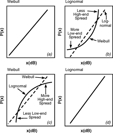
FIGURE 5.A.6 Weibull cdf shape on (a) Weibull and (b) lognormal scales, vs lognormal cdf shape on (c) Weibull and (d) lognormal scales.
Two Clutter Patch Measurements. Figure 5.A.7 shows measured ground clutter amplitude histograms and cdf’s from two clutter patches, a Peace River patch in part (a) at the top, and a Magrath patch in part (b) at the bottom. At both top and bottom, the cdf (read on the left ordinate of each plot) is shown plotted against a Weibull y-axis in the left plot and against a lognormal y-axis in the right plot. At the top, the same Peace River histogram is repeated both to left and right, and likewise for the Magrath histogram at the bottom (the percent of samples per histogram bin is read on the right ordinate of each plot). In either part (a) or part (b), for any given value of σ° on the x-axis, the same value of cumulative probability P(σ°) is read from the (left plot) Weibull scale or the (right plot) lognormal scale. The presentation format used in each of the four plots in Figure 5.A.7 is similar to that used for Figures 5.2 and 5.3, and Figures 5.14 and 5.15; this format is described more fully in the discussions relating to these preceding figures in the main body of Chapter 5. For example, the vertical dotted lines show the positions of the 50-, 70-, 90-, and 99-percentiles in each distribution; and the vertical dashed line shows the position of the mean in the distribution.
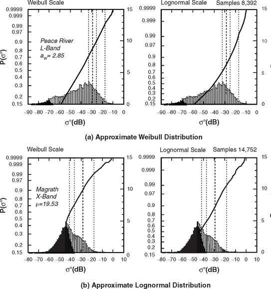
FIGURE 5.A.7 Two measured ground clutter amplitude distributions; (a) approximate Weibull distribution; (b) approximate lognormal distribution.
The upper part of Figure 5.A.7 [i.e., part (a)] shows the histogram and cdf resulting from an L-band measurement of a clutter patch at Peace River, Alberta. This Peace River patch was of agricultural land cover with a secondary component of trees (∼10% incidence of trees) and was observed at 0° depression angle. It was situated beginning at 3.9 km from the radar, and extended 4.1 km in range and 79.5° in azimuth. In this measurement, 4% of the samples are at radar noise level (black). The measurement was conducted at 150-m pulse length and vertical polarization. The lower part of Figure 5.A.7 [i.e., part (b)] shows the histogram and cdf resulting from an X-band measurement of a clutter patch at Magrath, Alberta. This Magrath patch was also of agricultural land cover (but in this case with only ∼1% incidence of trees) and was observed at 1° depression angle. It was situated beginning at 5.7 km from the radar, and extended 6.2 km in range and 46° in azimuth. In this measurement, 57.3% of the samples are at radar noise level. This measurement was also conducted at 150-m pulse length, but at horizontal polarization.
The Peace River cdf in part (a) of Figure 5.A.7 is extremely linear as plotted against the Weibull y-axis to the left, and hence shows upwards curvature plotted against the lognormal y-axis to the right (cf. Figure 5.A.6, top). Therefore, this measured distribution is accurately modeled as a Weibull distribution of shape parameter aw = 2.85 [this value of aw obtained through a regression analysis least-mean-squares fit of the cdf shown to the left in (a) to a straight line; see Appendix 2.B]. Many measured clutter cdf’s, while not as linear as (a) (left) on a Weibull axis, show some degree of upwards curvature like (a) (right) on a lognormal axis. The histogram in the upper plots is indeed of similar shape to the theoretical Weibull pdf shown in Figure 5.A.3 for aw = 3. The Magrath cdf in part (b) of Figure 5.A.7 is highly linear as plotted against the lognormal y-axis to the right, and hence shows downward curvature plotted against the Weibull y-axis to the left (cf. Figure 5.A.6, bottom). Therefore, this measured distribution is accurately modeled as a lognormal distribution with mean-to-median ratio ρ = 19.53 [also obtained through linear regression of the cdf shown to the right in (b), see Appendix 2.B]. Although not all measured clutter cdf’s are as linear on Weibull or lognormal axes as those shown in Figure 5.A.7 (a) (left) or (b) (right), considerably fewer measured clutter cdf’s show some degree of downwards curvature on a Weibull axis [like (b) (left)] than show some degree of upwards curvature on a lognormal axis [like (a) (right)]. That is, considerably more measured cdf’s tend towards Weibull curvature than towards lognormal curvature.
Table 5.A.2 shows additional statistical attributes relating to the Peace River and Magrath clutter measurements shown in Figure 5.A.7. The indicated measured values of sd/mean and mean/median of 5.5 and 11.1 dB, respectively, in the Peace River measured distribution compare relatively closely to the corresponding values of 6.0 and 11.5 dB that are applicable to an ideal analytic Weibull distribution of shape parameter aw = 2.85. This close comparison confirms the Weibull fit to be a good approximation to the Peace River clutter distribution, as does the high value of the coefficient of determination obtained in this fit, equal to 0.9993 (see Table 5.A.2). Similarly, the indicated measured values of sd/mean and mean/median of 10.7 and 13.2 dB, respectively, for the Magrath measurement shown in Table 5.A.2 compare reasonably well to the corresponding value of 12.9 dB applicable to each in an ideal analytic lognormal distribution of shape parameter ρ = 19.53.
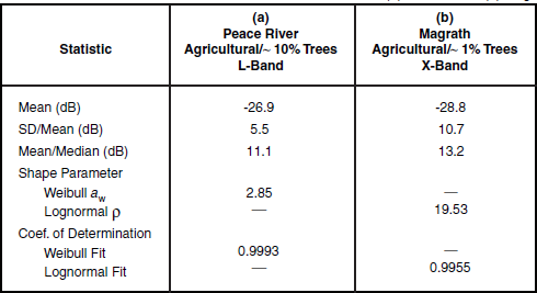
Note that, in a lognormal-like distribution [Table 5.A.2(b)], the values of sd/mean [theoretically equal to (ρ2−1)1/2; see Appendix 2.B] and mean/median (theoretically equal to ρ) are nearly equal for ρ >> 1; whereas, in a Weibull-like distribution [Table 5.A.2(a)], the value of mean/median far exceeds the value of sd/mean (see Figure 5.A.4). As with the Weibull fit in Figure 5.A.7(a), the lognormal fit in Figure 5.A.7(b) is confirmed by the reasonable comparison between measured and analytic values of sd/mean and mean/median and by the high value of the coefficient of determination applicable to this fit, equal to 0.9955 (see Table 5.A.2). Attempting to fit the Peace River distribution as lognormal (upper-right) or the Magrath distribution as Weibull (lower-left) results in gross mismatches between measured and analytic values of sd/mean and mean/median, and significantly lower values of coefficient of determination.
K-Distribution. The Weibull distribution is defined in Appendix 2.B and in Section 5.A.2 of this appendix. The lognormal distribution is defined in Appendix 2.B. It now remains to define the K-distribution. The cumulative distribution function (cdf) of the K-distribution is given by [3–5]
where Γ is the Gamma function and Kv is the modified Bessel function of second kind of order v. The parameter v is the shape parameter of the K-distribution; 1/d is a scale parameter. The first two moments of the K-distribution are
and
The K-distribution shape parameter v is given by
In this book, spread in distributions is often defined by the ratio of ![]() , where
, where ![]() and
and ![]() . An important relationship for the K-distribution is
. An important relationship for the K-distribution is
If spread in a Weibull distribution [from Eq. (5.A.5)] is equated with spread in a K-distribution [from Eq. (5.A.13)], the following equation is arrived at
that relates the Weibull shape parameter aw with the K-distribution shape parameter v.
Comparison of Analytic cdf Shapes. This section graphically compares the shapes of Weibull, lognormal, and K-distributions. In what follows, numerical plots of theoretical Weibull, lognormal, and K-cdf’s are provided to show how the previously introduced ideas of cdf curvature as plotted on Weibull and lognormal ordinates (see the notional diagrams, Figures 5.A.5 and Figures 5.A.6) develop in actual numeric data.27 The basis of the comparison is the same as used heretofore—namely, the median value x50 of the distribution is always set to x50 = 0.0001 (i.e., to −40 dB), and the spreads [i.e., ratios of ![]() or
or ![]() ] are those of Weibull distributions with values of shape parameter aw = 1, 2, 3, 4, 5. Table 5.A.3 shows expressions for the shape parameters for the Weibull, lognormal, and K-distributions, and the relationship of each to spread as given by
] are those of Weibull distributions with values of shape parameter aw = 1, 2, 3, 4, 5. Table 5.A.3 shows expressions for the shape parameters for the Weibull, lognormal, and K-distributions, and the relationship of each to spread as given by ![]() . Table 5.A.4 illustrates the distributions to be compared. The basic set of distributions are the Weibull distributions of x50 = 0.0001 and aw = 1, 2, 3, 4, 5. Table 5.A.4 shows the value of
. Table 5.A.4 illustrates the distributions to be compared. The basic set of distributions are the Weibull distributions of x50 = 0.0001 and aw = 1, 2, 3, 4, 5. Table 5.A.4 shows the value of ![]() for each one of these distributions. Then Table 5.A.4 shows the five values of ρ for the five corresponding lognormal distributions with the same values of
for each one of these distributions. Then Table 5.A.4 shows the five values of ρ for the five corresponding lognormal distributions with the same values of ![]() ; and similarly the five values of v for the five corresponding K-distributions.
; and similarly the five values of v for the five corresponding K-distributions.
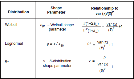
TABLE 5.A.4
Weibull, Lognormal, and K-Distribution Shape Parameters Corresponding to Weibull aw = 1,2,3,4,5
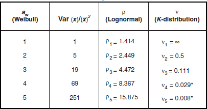
*Numerical results not provided.
Figure 5.A.8(a) shows the five basic Weibull distributions plotted against a Weibull y-axis.
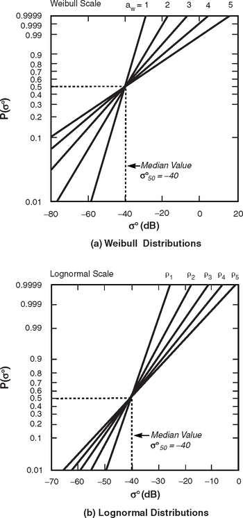
FIGURE 5.A.8 Weibull and lognormal distributions. (a) Weibull distributions on a Weibull scale; σ°50 = −40 dB, aw = 1, … 5. (b) Lognormal distributions on a lognormal scale; σ°50 = −40 dB; (sd/mean) for lognormal distributions = (sd/mean) for corresponding Weibull distributions of given aw.
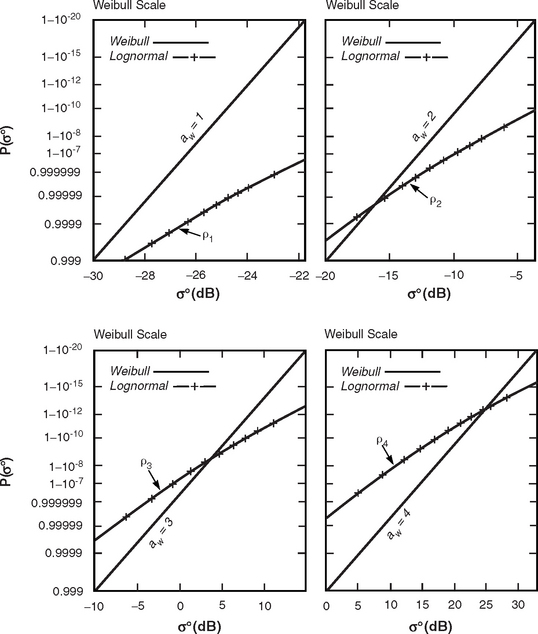
FIGURE 5.A.12 Weibull vs lognormal distributions, high tails, variable abscissas; Weibull scale; σ°50 = −40 dB, aw = 1, … 4; (sd/mean) for lognormal distribution = (sd/mean) for corresponding Weibull distribution of given aw.
Figure 5.A.8(b) shows the five corresponding lognormal distributions with values of ρ as given by Table 5.A.4 and of equal spread to the Weibull distributions, plotted against a lognormal y-axis. The lognormal distributions in Figure 5.A.8 are more tightly clustered than the Weibull distributions over the range shown because the lognormal spreads are more strongly affected by the lognormal high tails beyond the range plotted. That is, at high enough cumulative probability levels each lognormal distribution in Figure 5.A.8 eventually has a longer high tail than the corresponding Weibull distribution. This will be seen in what follows.
Figure 5.A.9 plots equivalent Weibull, lognormal, and K-distributions on Weibull y-axes for σ°50 = −40 dB, and for the first three values of spread specified in Table 5.A.4. The upward and downward curvatures sketched in Figure 5.A.5 are evident in Figure 5.A.9. Note that the K-distribution corresponding to aw = 1 (i.e., v = ∞) degenerates to negative exponential (or Rayleigh voltage) as does the Weibull for aw = 1; and the K-distribution corresponding to aw = 2 (i.e., v = 0.5) also is identically equal to the Weibull distribution of aw = 2. For the aw = 3 plot in Figure 5.A.9, the curvatures are as sketched in Figure 5.A.5.

FIGURE 5.A.9 Weibull vs lognormal vs K-distributions; Weibull scale; σ°50 = −40 dB; aw = 1,2,3; (sd/mean) for lognormal and K-distributions = (sd/mean) for corresponding Weibull distributions of given aw.
Figure 5.A.10 shows the five basic Weibull and five basic lognormal distributions, each with σ°50 = −40 dB and with values of sd/mean as specified in Table 5.A.4, in which each distribution is plotted against a Weibull y-axis. These plots show each Weibull distribution to be a straight line as required when plotted against a Weibull probability ordinate (see Appendix 2.B), and show each lognormal distribution to be of downwards curvature as indicated in the sketch of Figure 5.A.6(c) [compare also with the measured data in Figure 5.A.7(a) (left) and (b) (left)]. Figure 5.A.11 shows the same Weibull and lognormal distributions as in Figure 5.A.10, but here plotted against a lognormal y-axis. These plots show each lognormal distribution to be a straight line as required when plotted against a lognormal probability ordinate (see Appendix 2.B), and show each Weibull distribution to be of upwards curvature as indicated in the sketch of Figure 5.A.6(b) [compare also with the measured data in Figure 5.A.7(a) (right) and (b) (right)]. Considerably more low-angle measured clutter data tend to be Weibull-like or quasi-Weibull (i.e., displaying a significant degree of upwards curvature when plotted against lognormal ordinates, as shown by the Weibull plots in Figure 5.A.11), than appear to be lognormal-like or quasi-lognormal (i.e., displaying a significant degree of downwards curvature when plotted against Weibull ordinates, as shown by the lognormal plots in Figure 5.A.10).
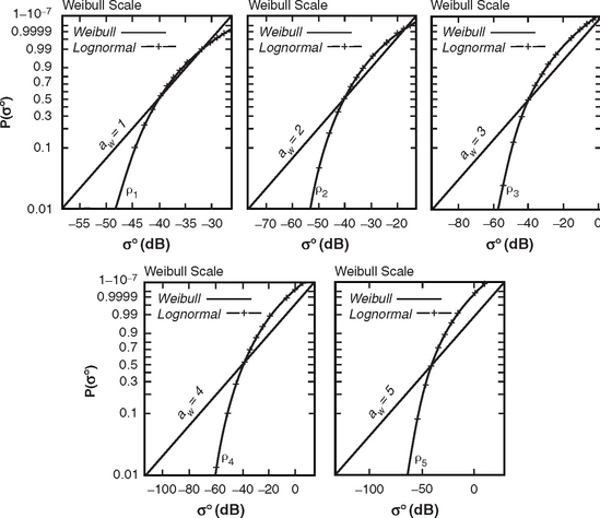
FIGURE 5.A.10 Weibull vs lognormal distributions; Weibull scale, variable abscissas; σ°50 = −40 dB, aw = 1, … 5; (sd/mean) for lognormal distribution = (sd/mean) for corresponding Weibull distribution of given aw.
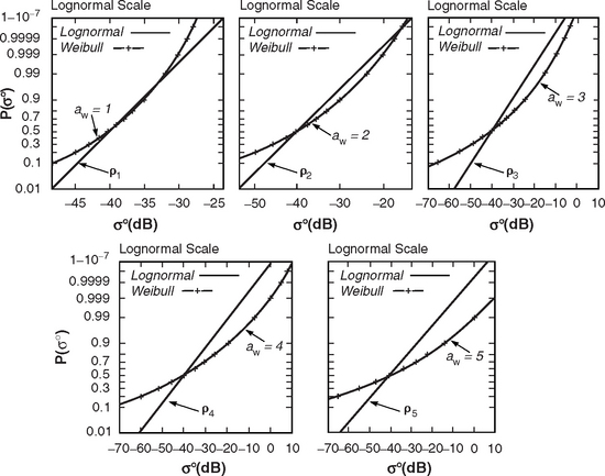
FIGURE 5.A.11 Lognormal vs Weibull distributions; lognormal scale; σ°50 = −40 dB, aw = 1, … 5; (sd/mean) for lognormal distribution = sd/mean) for corresponding Weibull distribution of given aw.
In Figures 5.A.10 and Figures 5.A.11, the crossover points in the high-end distribution tails where the lognormal distribution starts to extend to higher values of σ° compared with the Weibull [see Figures 5.A.6(c) and (b)] only explicitly appear in the first two plots of each figure. Figure 5.A.12 shows the first four of the five basic Weibull and five basic lognormal distributions (see Table 5.A.4) plotted to very high values of cumulative probability to better show the behavior of the high-end tails. It is apparent in these plots that, at high enough probability levels, the lognormal distribution always reaches to higher values of σ° (i.e., always has a longer high-end tail) than the corresponding Weibull distribution, for a given ratio of sd/mean.
5.A.4 FITS TO MEASURED FARMLAND CLUTTER: WEIBULL VS LOGNORMAL VS K-
Many distributions have been proposed in the literature to model the amplitude pdf of spiky clutter; see, for example [1, 3–13]. This section provides results from a study (for which [14] is a summary) of two particular experiments of Phase One ground clutter that show that in these data Weibull statistics usually (but not without occasional exception) provide better fits to the clutter amplitude distributions than do lognormal or K-distributions.28
Other results from this study are discussed in Chapter 4, Section 4.6.3, under the heading “Spatial Correlation.” In this study, the term clutter amplitude refers to the clutter voltage amplitude, that is, to the square root of the sum of the squares of the I and Q voltage components. In what follows, the empirical pdf is compared with the Weibull, lognormal, and K- pdf’s having the same first- and second-order moments, and with the Rayleigh pdf having the same variance. Additional details are available in [14], including expressions for the first- and second-order moments of the Weibull, lognormal, and K- pdf’s ([12, 15]; see also Appendix 2.B).
The two clutter experiments studied were of open farmland X-band clutter obtained at the clutter measurement site of Wolseley, Saskatchewan; one experiment is at VV-polarization, the other at HH-polarization. Both experiments are of Phase One survey data taken in slow scan mode (see Chapter 3) through one ∼90° azimuth sector in which 703 azimuth samples were collected per range cell. Each experiment contains four range intervals, and each range interval contains 316 range cells of 15-m sampling interval. Thus each range interval covers 4.74 km, and the four contiguous range intervals cover from 1 to 20 km. Figure 5.A.13 shows a three-dimensional clutter map covering the first range interval at VV-polarization; the spiky nature of the discrete farmland clutter is evident.
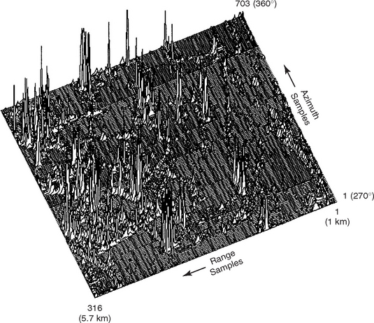
FIGURE 5.A.13 3D clutter map of clutter spatial amplitude statistics from open farmland. 1st range interval; VV-polarization. (Results provided by F. Gini and M. Greco, Univ. of Pisa. After [14]; by permission, © 1999 IEEE.)
Figure 5.A.14 shows the histogram of the I component of the clutter voltage signal from the fourth range interval at VV-polarization—the histogram of the Q component is similar. Long, drawn-out, slowly diminishing tails are evident in the histogram of Figure 5.A.14. The histogram (or empirical pdf) of Figure 5.A.14 is compared in the figure with the Gaussian pdf having the same variance as the empirical pdf and zero mean (the very small, residual dc offset of each measured channel was estimated in each range interval and subtracted from the data). It is apparent that the I (and Q) components of spatially varying clutter amplitudes do not follow Gaussian distributions (i.e., the voltage amplitude is not Rayleigh, and the clutter strength distribution is not exponential). An X-band histogram and cumulative distribution of clutter strength σ°F4 from a clutter patch at this same Wolseley site were shown previously in Figure 5.15 of Chapter 5; these data of Figure 5.15 appear to be well modeled as a Weibull distribution. To be determined here is if this previous indication of Weibull is borne out in the following more analytically rigorous results.
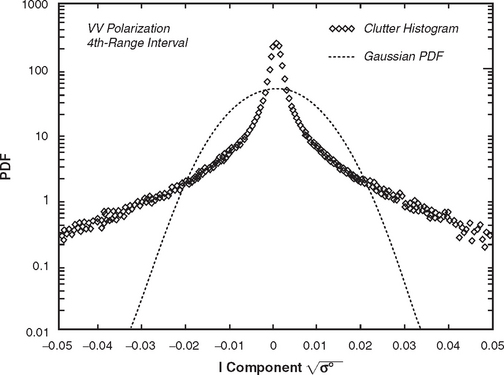
FIGURE 5.A.14 Histogram of I component of clutter spatial amplitude statistics from open farmland. (Results provided by F. Gini and M. Greco, Univ. of Pisa. After [14]; by permission, © 1999 IEEE.)
Figure 5.A.15 plots clutter amplitude histograms for the second and fourth range intervals, both at HH-polarization, and compares them with Rayleigh, Weibull, lognormal, and K-distributions. In this figure, the measured pdf is compared with the Weibull, lognormal, and K- pdf’s having the same first and second order moments, and with the Rayleigh pdf having the same variance. For the second range interval (a), the data are very well fitted by the Weibull approximation over the full range of amplitudes shown. For the fourth interval (b), the data appear to generally lie between the Weibull and lognormal approximations.
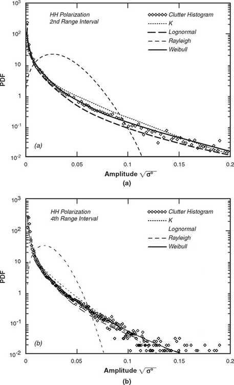
FIGURE 5.A.15 Histograms of clutter spatial amplitude statistics from open farmland. (a) 2nd range interval; (b) 4th range interval. (Results provided by F. Gini and M. Greco, Univ. of Pisa. Part (b) after [14]; by permission, © 1999 IEEE.)
Figure 5.A.16 shows an X-band clutter amplitude histogram obtained as temporal variations from a fixed cell containing windblown trees. These data were obtained at the Katahdin Hill measurement site; they constitute long-time-dwell data (see Chapter 3) in which 30,720 samples per cell were recorded at 500 Hz PRF (stationary antenna, VV-polarization; 15-m pulse length). These temporal data are shown here to indicate the profound differences in clutter statistics that result when the clutter is collected as spatial variations over many cells of open farmland, on the one hand (Figure 5.A.15), and as temporal variations from windblown foliage, on the other (Figure 5.A.16). The temporal data in Figure 5.A.16 very closely follow the Rayleigh distribution—the I and Q components of these data follow Gaussian pdf’s as shown in Figure 5.A.14. The theoretical Rayleigh pdf in Figure 5.A.16 which the empirical data so closely follow is normalized to have the same variance as the data.
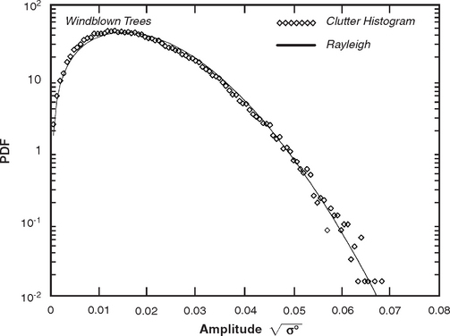
FIGURE 5.A.16 Histogram of clutter temporal amplitude statistics from a cell containing windblown trees. (Results provided by F. Gini and M. Greco, Univ. of Pisa. After [14]; by permission, © 1999 IEEE.)
For the Wolseley farmland spatial clutter data, Figure 5.A.17 shows the first six normalized moments as computed from the data and compares them to the theoretical higher moments of Weibull, lognormal, and K-distributions [12, 14, 15]. In these results, the parameters of the theoretical distributions are set by matching the first two moments of the theoretical distributions to the first two computed moments in the empirical clutter data. As in Figure 5.A.15, results are shown for the second and fourth range intervals at HH-polarization. For the second range interval (a), all four higher moments of orders 3, 4, 5, and 6 computed in the measured data match those of the Weibull distribution very closely—in fact, the measured moments actually overlay the Weibull theoretical moments in this plot. For the fourth range interval (b), the four higher moments computed in the measured data lie between the corresponding Weibull and lognormal moments—but somewhat more closely to Weibull. These results substantiate what initially appears to be true in the histograms of Figure 5.A.15. Note in Figure 5.A.17 that Weibull higher moments lying between lognormal and K-distribution higher moments shows in another way how Weibull distributions lie intermediate between lognormal and K-distributions in terms of degree of spread involved (compare with the figures showing distribution shape in Section 5.A.3).
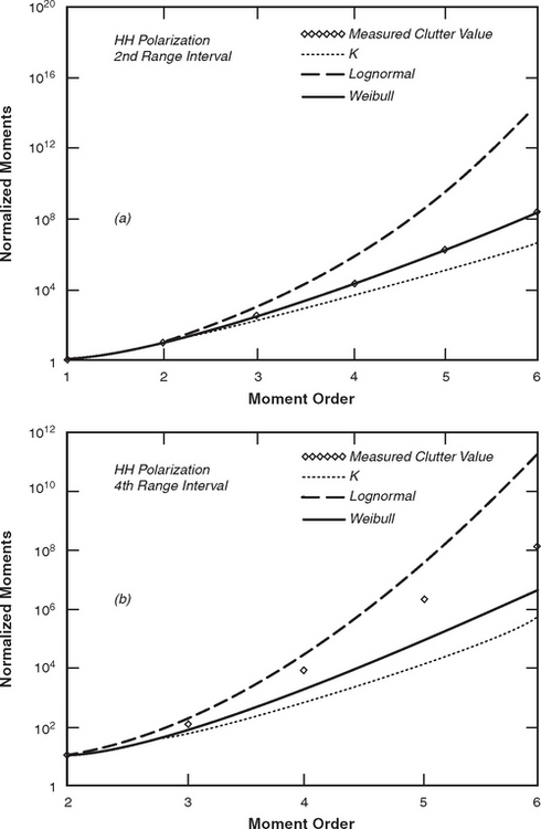
FIGURE 5.A.17 Normalized moments of clutter spatial amplitude distributions from open farmland. (a) 2nd range interval; (b) 4th range interval. (Results provided by F. Gini and M. Greco, Univ. of Pisa. Part (b) after [14]; by permission, © 1999 IEEE.)
Figure 5.A.18 plots the measured cdf’s, here for the third and fourth range intervals both at HH-polarization, on Weibull paper. The Weibull paper utilized is such that the abscissa is ![]() , and the ordinate is
, and the ordinate is ![]() . In such a plot, a Weibull distribution for clutter amplitude
. In such a plot, a Weibull distribution for clutter amplitude ![]() plots as a straight line with slope given by the shape parameter of the Weibull distribution [14]. These matters are explained more fully in Appendix 2.B.
plots as a straight line with slope given by the shape parameter of the Weibull distribution [14]. These matters are explained more fully in Appendix 2.B.
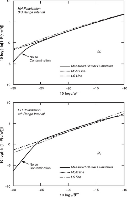
FIGURE 5.A.18 Cumulative clutter spatial amplitude distributions plotted on Weibull paper. (a) 3rd range interval; (b) 4th range interval. (Results provided by F. Gini and M. Greco, Univ. of Pisa. Part (b) after [14]; by permission, © 1999 IEEE.)
The empirical cdf for the third range interval is quite linear when plotted on the Weibull paper of Figure 5.A.18(a), indicating that a Weibull distribution accurately fits these data. The empirical cdf for the fourth range interval is also quite linear in Figure 5.A.18(b). In Figure 5.A.18, each measured clutter cumulative or cdf is compared with the method of moments (MoM) line representing the Weibull cdf with the same mean and mean square values as the measured data, and with the line obtained by linear least squares (LS) fitting to the data [16]. For each range interval, it is apparent in Figure 5.A.18 that the MoM and LS techniques provide very similar values for coefficients (i.e., slope, intercept) of Weibull distributions to match the measured cdf’s.
Note that the Weibull distributions shown in Figure 5.A.18 are for the clutter amplitude ![]() ; the shape parameter aw for the corresponding cdf of clutter strength σ° is twice that obtained directly from Figure 5.A.18. Thus, the LS value of aw applicable to the σ° cdf in both (a) and (b) of Figure 5.A.18 is aw = 4.55.29 This value compares closely with the value pertaining to the Wolseley data of Figure 5.15, viz., aw = 4.7 (see Table 5.12), for which the applicable clutter patch straddles the first and second range intervals. In both parts (a) and
; the shape parameter aw for the corresponding cdf of clutter strength σ° is twice that obtained directly from Figure 5.A.18. Thus, the LS value of aw applicable to the σ° cdf in both (a) and (b) of Figure 5.A.18 is aw = 4.55.29 This value compares closely with the value pertaining to the Wolseley data of Figure 5.15, viz., aw = 4.7 (see Table 5.12), for which the applicable clutter patch straddles the first and second range intervals. In both parts (a) and
(b) of Figure 5.A.18, the regions where the data tails off at the left are the result of radar noise contamination and should be ignored.
A goodness-of-fit hypothesis test was applied to each of the eight sets of Wolseley X-band farmland clutter data—i.e., four range intervals, two polarizations. This test determines which distribution, Weibull, lognormal, or K-, best fits each set of data. Over their complete extents, measured low-angle clutter distributions almost never pass rigorous statistical hypothesis tests for belonging to any practicable theoretical distribution. Therefore, a modified Kolmogorov-Smirnoff test was employed such that only the data in the upper tail region ![]() was taken into account. The test is characterized by the parameter α that represents the probability of Type I error. Probability of Type I error is the probability of error that occurs in rejecting the null hypothesis when true. Here, the null hypothesis is that the measured (empirical) clutter distribution is equal to the hypothesized theoretical distribution under test. If this probability is low, the hypothesis that the empirical distribution is equal to the theoretical distribution should be rejected; if this probability is high, this same hypothesis should be accepted [17]. Results are shown in Table 5.A.5. The high probabilities under Weibull indicate that all eight data sets are reasonably well fitted by Weibull distributions in the region
was taken into account. The test is characterized by the parameter α that represents the probability of Type I error. Probability of Type I error is the probability of error that occurs in rejecting the null hypothesis when true. Here, the null hypothesis is that the measured (empirical) clutter distribution is equal to the hypothesized theoretical distribution under test. If this probability is low, the hypothesis that the empirical distribution is equal to the theoretical distribution should be rejected; if this probability is high, this same hypothesis should be accepted [17]. Results are shown in Table 5.A.5. The high probabilities under Weibull indicate that all eight data sets are reasonably well fitted by Weibull distributions in the region ![]() , some very closely. Only in three cases is the lognormal probability higher than Weibull, but the Weibull probability is still high in each of these three cases. Some of the lognormal probabilities are very low. All of the K-distribution probabilities are low or very low, indicating that none of the eight distributions are well fitted by K-distributions in their upper tails.
, some very closely. Only in three cases is the lognormal probability higher than Weibull, but the Weibull probability is still high in each of these three cases. Some of the lognormal probabilities are very low. All of the K-distribution probabilities are low or very low, indicating that none of the eight distributions are well fitted by K-distributions in their upper tails.
TABLE 5.A.5
Results of Kolmogorov-Smirnoff Hypothesis Test Modified to Upper Tail Region ![]() of Clutter Spatial Amplitude Distribution*
of Clutter Spatial Amplitude Distribution*
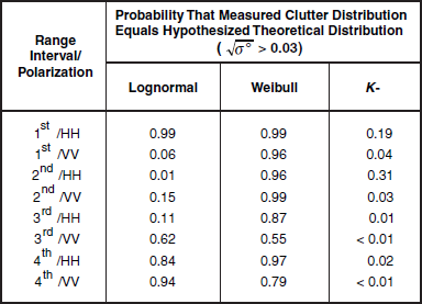
*Results provided by F. Gini and M. Greco, Univ. of Pisa. After [14]; by permission, © 1999 IEEE.
As a result of the various preceding analyses of the empirical Wolseley farmland spatial clutter amplitude distributions provided in Section 5.A.4, it is evident that, in the first and second range intervals, these clutter data are accurately represented and much better fitted by Weibull distributions than by lognormal or K-distributions. In the third and fourth range intervals, the empirical data show behavior intermediate between Weibull and lognormal.
REFERENCES
1. Billingsley, J. B., Larrabee, J. F. “Multifrequency Measurements of Radar Ground Clutter at 42 Sites,”; Volumes 1, 2, 3. MIT Lincoln Laboratory, Technical Rep. 916, Lexington, MA, 15 November 1991. [DTIC AD-A246710. ].
2. Nathanson, F. E., Reilly, J. P., Cohen, M. N. Radar Design Principles, 2nd ed. New York: McGraw-Hill, 1991.
3. Barton, D. K. Modern Radar System Analysis. Norwood, MA: Artech House, 1988.
4. Long, M. W. Radar Reflectivity of Land and Sea, 3rd ed. Boston: Artech House, 2001.
5. Skolnik, M. I. Introduction to Radar Systems, 3rd ed. New York: McGraw-Hill, 2001.
6. Billingsley, J. B. “Radar ground clutter measurements and models, part 1: Spatial amplitude statistics,”. In: AGARD Conf. Proc. Target and Clutter Scattering and Their Effects on Military Radar Performance. Ottawa: ; 1991. [AGARD-CP-501, DTIC AD-P006 373. ].
7. H. C. Chan, “Radar ground clutter measurements and models, part 2: Spectral characteristics and temporal statistics,” AGARD Conference Proceedings on Target and Clutter Scattering and Their Effects on Military Radar Performance, AGARD-CP-501 (1991).
8. G. C. Sarno, “A model of coherent radar land backscatter,” AGARD Conference Proceedings on Target and Clutter Scattering and Their Effects on Military Radar Performance, AGARD-CP-501 (1991).
9. S. P. Tonkin and M. A. Wood, “Stochastic model of terrain effects upon the performance of land-based radars,” AGARD Conference Proceedings on Target and Clutter Scattering and Their Effects on Military Radar Performance, AGARD-CP-501 (1991).
10. Sekine, M., Mao, Y. Weibull Radar Clutter. London, U. K. : Peter Peregrinus Ltd. and IEE, 1990.
11. R. R. Boothe, “The Weibull Distribution Applied to the Ground Clutter Backscatterer Coefficient,” U. S. Army Missile Command Rept. No. RE-TR-69-15, Redstone Arsenal, AL, June 1969; DTIC AD-691109.
12. Warden, M. P., Dodsworth, E. J. “A Review of Clutter, 1974,”. In: Royal Radar Establishment Technical Note No. 783. U. K. : Malvern; September 1974. [DTIC AD A014421. ].
1. Sekine, M., Mao, Y. Weibull Radar Clutter. London, U. K. : Peter Peregrinus Ltd. and IEE, 1990.
2. Blake, L. V. Radar Range-Performance Analysis, 2nd ed. Silver Spring, MD: Monroe Publishing, 1991.
3. Jakeman, E. “On the statistics of. K-distributed noise,” J. Physics A: Math. Gen.. 1980; Vol. 13:31–48.
4. Jao, J. K. “Amplitude distribution of composite terrain radar clutter and the. K-distribution,” IEEE Trans. Ant. Prop.. October 1984; Vol. AP-32(no. 10):1049–1062.
5. Ward, K. D. “Application of the K-distribution to radar clutter—A review,”. In: Proc. Internat. Symp. on Noise and Clutter Rejection in Radars and Imaging Sensors. Tokyo: IEICE; 1989:15–21.
6. Holliday, E. M., Wood, E. W., Powell, D. E., Basham, C. E. “L-Band Clutter Measurements,”. In: U. S. Army Missile Command Report RE-TR-65-1. : Redstone Arsenal, AL; November 1964. [DTIC AD-461590. ].
7. Nathanson, F. E., Reilly, J. P. “Clutter statistics that affect radar performance analysis,”. EASCON Proc. (supplement to IEEE Trans.). November 1967; Vol. AES-3(no. 6):386–398.
8. W. L. Simkins, V. C. Vannicola, and J. P. Ryan, “Seek Igloo Radar Clutter Study,” Rome Air Development Center, Technical Rep. RADC-TR-77-338, October 1977. Updated in FAA-E-2763b Specification, Appendix A, May 1988. See also FAA-E-2763a, September 1987; FAA-E-27263, January 1986, July 1985.
9. Anastassopoulos, V., Lampropoulos, G. A. “High resolution radar clutter classification,”. In: Proceedings of IEEE International RADAR Conference. Washington, DC: ; May 1995:662–666.
10. Chan, H. C. “Radar sea-clutter at low grazing angles,”. IEE Proceedings, Pt. F. Apr. 1990; 137(2):102–112.
11. Chen, K. S., Fung, A. K. “Frequency dependence of backscattered signals from forest components,”. IEE Proceedings, Pt. F. Dec. 1995; 142(6):310–315.
12. Nohara, T. J., Haykin, S. “Canadian East Coast radar trials and the K-distribution,”. IEE Proceedings, Pt. F. Apr. 1991; 138(2):80–88.
13. Menon, K. Rajalakshmi, Balakrishnan, N., Janakiraman, M., Ramchand, K. “Characterization of fluctuating statistics of radar clutter for Indian terrain,”. IEEE Transactions on Geoscience and Remote Sensing. Mar. 1995; Vol. 33(no. 2):317–323.
14. Billingsley, J. B., Farina, A., Gini, F., Greco, M. V., Verrazzani, L. “Statistical analyses of measured radar ground clutter data,”. IEEE Trans. AES. Vol. 35(no. 2), April 1999.
15. Stuart, A., Ord, J. K. Kendall’s Advanced Theory of Statistics. London: Griffin, 1987.
16. Kay, S. M. Fundamentals of Statistical Signal Processing: Estimation Theory. Englewood Cliffs, NJ: Prentice-Hall, 1993.
17. Kim, P. J., Jennrick, R. I., “Tables of the exact sampling distribution of the two sample Kolmogorov-Smirnoff criterion Dmn(m<n). ”Harter, H. L., Owen, D. B., eds. Selected Tables in Mathematical Statistics, Vol. 1. Providence, RI: American Mathematical Society, 1973.
26.All Chapter 5 figures occur consecutively in the figures-only, color section beginning on page 447.
27.Digitized terrain elevation data may be acquired from the U. S. Geological Survey (USGS) or the U. S. National Imagery and Mapping Agency (NIMA). Such data are called Digital Elevation Models (DEMs) by USGS, and Digital Terrain Elevation Data (DTED) by NIMA. In the past, the data from both sources were commonly available at 3 arc-seconds (i.e., ≈100 m) sampling interval, but data at smaller sampling intervals (e.g., 1 arc-second) are now increasingly available.
28.These seven clutter patches were all within line-of-sight visibility to the radar on the real earth.
26.That is, from the underlying information for this terrain/depression angle category corresponding to that shown in Table 5.2.
27.These results, shown in Figures 5.A.8–5.A.12, were generated by Mr. Tejan K. Tingling who at the time was an undergraduate student from Norfolk State University, Norfolk, VA, participating in the Lincoln Laboratory Summer Internship Program.
28.The summary provided here includes material originally published in [14], by permission of IEEE.
29.Table IV in [14] gives Weibull shape parameter c = 0.44 for both empirical ![]() cdf’s in Figure 5.A.18; aw = 2/c.
cdf’s in Figure 5.A.18; aw = 2/c.