
APPROACHES TO CLUTTER MODELING
4.1 INTRODUCTION
The historical technical literature on low-angle land clutter includes a number of different past approaches for attempting to model this complex phenomenon, as reviewed in Chapter 1. Thus, most simply, low-angle clutter has been characterized as a single-variable characteristic or functional relationship between the dependent variable σ° and any one of the following three independent variables: (1) illumination angle to the backscattering terrain point; (2) radar carrier frequency; and (3) range to the backscattering terrain point. Chapters 2 and 3 illustrate at some length the strong dependencies of low-angle clutter on illumination (i.e., depression) angle and radar carrier frequency based on Phase Zero X-band data and Phase One five-frequency repeat sector data, respectively.
Although providing new useful clutter modeling information, the results of Chapters 2 and 3 in themselves do not constitute a clutter model generalized to be applicable to any surface-sited radar. The objective of such a model is to provide a description of the amplitude statistics of the clutter returns received by an arbitrary radar in a specified environment. As has been discussed previously in this book, the mean strength (first moment) of the clutter amplitude distribution depends strongly on (1) depression angle and (2) radar frequency. However, the equally important shape parameter (derived from the ratio of second to first moments) of the clutter amplitude distribution is fundamentally dependent on the spatial resolution of the radar. The modeling information of Chapters 2 and 3 is restricted to Phase Zero and Phase One pulse lengths and beamwidths. As such, this modeling information may be used to replicate clutter in radars of Phase Zero or Phase One spatial resolution, but is not generalized there to be applicable to radars of spatial resolution significantly different from the Phase Zero and Phase One radars.
Chapter 4 provides an interim angle-specific clutter model fully generalized to be applicable to radars of arbitrary spatial resolution. This interim model is presented in Section 4.2. It is based on the Phase Zero X-band database (Chapter 2) and the Phase One repeat sector database (Chapter 3) and includes all important trends of variation of low-angle clutter amplitude statistics seen in these two databases, including the general dependency of shape parameter on the spatial resolution or cell size of the radar. The interim clutter model is thus a complete model applicable to any surface-sited radar in any ground environment. This model is labelled “interim” because it does not have the statistical depth of the spatially comprehensive 360° Phase One survey data. The identical structure of the interim clutter model carries forward to the more comprehensive modeling information of Chapter 5 which is based on the Phase One survey data.
The presentation of material in Chapter 4 is as follows. First, Section 4.1.1 describes an important clutter modeling objective, namely, the prediction or simulation of plan-position indicator (PPI) clutter maps in surface-sited radars. Then Section 4.1.2 discusses the clutter modeling rationale of this book, distinguishing between angle-specific clutter modeling information suitable for site-specific clutter prediction using digitized terrain elevation data (DTED) and non-angle-specific modeling information suitable for more generic clutter prediction. Section 4.1.3 discusses clutter as a statistical random process and briefly describes the scope of included material within the context of available random-process statistical attributes. Section 4.2 presents the angle-specific interim clutter model, which requires specification of the depression angle to each clutter patch. This model explicitly incorporates the interdependent effects on clutter of (1) depression angle and (2) radar frequency, but the effects of (3) range occur implicitly in its site-specific application whereby the occurrences of visible clutter patches decrease with increasing range at each specific site.
PPI clutter maps in surface-sited radars are inherently patchy in character. The details of the patchiness are specific to each site. There remains a need, however, for a generic non-site-specific approach to clutter modeling in which the spatial character of the clutter field is not patchy. An important feature of a PPI clutter map for a surface-sited radar, disregarding the specificities of patchiness in each such map, is the obvious dissipation of the clutter with increasing range. Section 4.3 takes up the subject of non-angle-specific clutter modeling information suitable for use in non-patchy prediction. This naturally leads to the explicit introduction of (3) range as the important independent variable affecting the clutter, in contrast to effects of range occurring implicitly in site-specific modeling. What becomes apparent based on clutter measurements at many sites is that the occurrence of clutter fundamentally depends upon (i.e., decreases with) range, for a given site height; and that the strength of the clutter where it occurs is fundamentally dependent upon terrain type but not upon range. Section 4.3 provides a simple, generic, non-patchy clutter model based upon these observations in the measurement data.
Section 4.4 discusses the intimate interrelationship at low angles between geometrically visible terrain and clutter occurrence. Section 4.5 discusses the difficulties involved at low angles in attempting to distinguish discrete from distributed clutter and takes up the issue of how best to reduce the measurement data. Section 4.6 provides additional insight into the clutter phenomenon and the ramifications in its modeling by providing brief introductory discussions of its temporal statistics, its spectral characteristics, and its correlative properties. Section 4.7 summarizes many of the insights developed in Chapter 4. Appendices 4.A, 4.B, and 4.C further develop the effects of radar height and range in low-angle clutter and discuss the complications introduced by range-dependent sensitivity limitations and the corresponding range-dependent effects of radar noise corruption in clutter measurement data. Appendix 4.D describes a more computationally intensive approach to low-angle clutter modeling in which spatial cells that are locally strong (i.e., “discretes”) compared to their neighbors are modeled separately from the weaker neighboring (i.e., “background”) cells.
4.1.1 MODELING OBJECTIVE
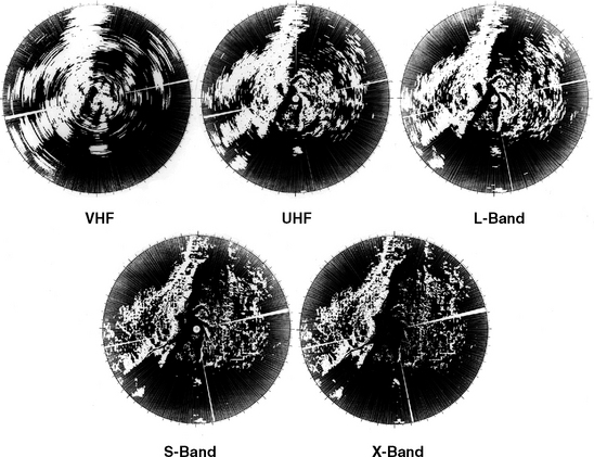
Figure 4.1 shows measured PPI ground clutter maps for all five Phase One frequencies at the Peace River South measurement site, located high on the east bank of the Peace River in Alberta. The maximum range in these maps is 23 km; north is at zenith. Clutter is shown as white where σ°F4 > −40 dB. These five-frequency Peace River clutter maps may be compared with the five-frequency Gull Lake West clutter maps previously shown in Figure 3.9. To the west in each map in Figure 4.1 is the well-illuminated river valley; to the east, level terrain is illuminated at grazing incidence. As with the Gull Lake West measurements, as patterns of spatial occurrence of ground clutter, all five clutter maps at Peace River are quite similar. As previously discussed, the reason for this similarity is that the relatively strong clutter shown in Figure 4.1 largely comes from visible terrain. At all five frequencies in the figure, the nature of the clutter tends to be granular and patchy. However, the granularity is greater at grazing incidence to the east, less at the higher depression angles to the west. Also as has been discussed, such effects are principally due to depression angle as it affects microshadowing. Obvious in Figure 4.1 is the effect of increasing beamwidth with decreasing frequency causing increased azimuthal smearing of the clutter. This effect is of spatial resolution, such that decreasing resolution results in decreased spreads in clutter amplitude distributions.
A main modeling objective of this book is the site-specific prediction of clutter maps such as those shown in Figure 4.1 using DTED. This objective is illustrated by Figure 4.2 which compares predicted terrain visibility and measured X-band clutter at Katahdin Hill,

Massachusetts. To the left is predicted terrain visibility with a 5-m antenna on the basis of geometric line-of-sight visibility in DTED. To the right is the measured Phase Zero clutter map at the same site. In approximate measure, the two spatial patterns are quite similar;24 this similarity is borne out in the plot showing percent circumference visible compared with percent circumference in measured clutter vs range. DTED are used to deterministically predict where the clutter occurs, and a statistical depression-angle-specific and terrain-type-specific clutter model is used to predict the strength of the clutter in each visible cell.
The interim clutter model presented in Section 4.2 is suitable for such site-specific clutter prediction as well as other applications. The interim clutter model structure is illustrated by the schematic diagram of Figure 4.3. To model site-specific clutter, Weibull random numbers are distributed cell-by-cell over visible terrain as determined by DTED. As indicated in Figure 4.3, the Weibull numbers are drawn from distributions characterized by a Weibull mean strength ![]() and a Weibull shape parameter aw. These two coefficients vary with terrain type, depression angle, and the important radar parameters of frequency and resolution. Mean strength
and a Weibull shape parameter aw. These two coefficients vary with terrain type, depression angle, and the important radar parameters of frequency and resolution. Mean strength ![]() varies with frequency, aw varies with resolution, and both
varies with frequency, aw varies with resolution, and both ![]() and aw vary with depression angle and terrain type. The actual interim clutter model matrix of numbers organized as shown in Figure 4.3 is provided in Section 4.2.
and aw vary with depression angle and terrain type. The actual interim clutter model matrix of numbers organized as shown in Figure 4.3 is provided in Section 4.2.


4.1.2 MODELING RATIONALE
Low-angle ground clutter is a patchy phenomenon. Areas of the ground that are directly visible to the radar usually cause relatively strong clutter returns, and areas of the ground that are shadowed or masked to the radar usually cause relatively weak clutter returns, often below the sensitivity of the radar. Using DTED allows the deterministic prediction and distinction between macroregions of general geometric visibility and macroregions of shadow, where macro implies kilometer-sized regions that encompass hundreds or thousands of spatial resolution cells. Such deterministic prediction of the specific pattern of spatial occurrence of ground clutter at a given site is essentially what is meant here by site-specific study.
Predicting, in this manner, the existence of a macropatch of clutter at some site, a description is subsequently needed of the statistics of the clutter returns that are expected from within the patch. Thus Section 4.2 provides modeling information to describe clutter amplitude distributions occurring over macrosized spatial regions of visible terrain. These distributions are characterized by broad spread. The degree of spread in the distribution is fundamentally controlled by depression angle, that is, the angle below the horizontal at which the patch is observed at the radar. Depression angle is a quantity that can be computed relatively rigorously and unambiguously from DTED, depending as it does simply on range and relative elevation difference between the radar antenna and the patch. The fundamental dependence of spread in the clutter amplitude distribution on depression angle is significant even for the very low depression angles (i.e., typically < 1°) and small patch-to-patch differences in depression angle (i.e., typically fractions of 1°) that occur in surface-sited radar. The patch-specific modeling information for ground clutter amplitudes presented in Section 4.2 is tied tightly to this basic dependence on depression angle, such that amplitude distributions are specified in terms of small and precise gradations of depression angle for various terrain types.
Let us reflect on this approach to modeling low-angle ground clutter. As a physical phenomenon, the most salient attribute of low-angle ground clutter is variability. This variability is manifested in two important ways: first, as patchiness in spatial occurrence and second, as extremely wide cell-to-cell statistical fluctuation in strength (i.e., spikiness) within a patch. Concerning spatial patchiness, it is emphasized that clutter does not always exist, and it is the patch-specific on-again, off-again macrobehavior of clutter that at first level determines the performance of a given radar against a given low-altitude aircraft at a given site. Concerning wide cell-to-cell variations of clutter strength within macropatches, it is emphasized that what appears at first consideration to be a phenomenon of extreme variability and little predictability turns out in the end, after much data analysis, to be generally dependent on very fine differences in depression angle.
Use of site-specific DTED allows the capture of both these basic attributes of low-angle ground clutter, its spatial patchiness (approximately computed simply as geometric visibility), and (through depression angle) its expected range of amplitudes within a patch. Therefore, this approach to modeling low-angle clutter is regarded as a major advance over more general non-patchy approaches that do not distinguish between macroregions of clutter occurrence and macroregions of shadow. This approach allows an analyst to predict, within macroregions, where a surface-sited radar can be expected to encounter clutter interference and where the radar will be free of such interference; and, given that the radar is experiencing clutter, what, on the average, the expected statistics of signal-to-clutter ratio will be across the macroregion of clutter.
Clutter returns within patches are often highly spatially correlated. This book discusses the fact that the dominant clutter sources within macroregions of general geometric visibility are usually spatially localized or discrete, such that groups of cells providing strong returns are often separated by cells providing weak or noise-level returns. The occurrence of noise-level returns distributed within macroregions of general geometric visibility is referred to as “microshadowing,” where micro implies resolution-cell-sized areas (see Figure 2.11 and its accompanying discussion in Chapter 2). The high degree of spatial microcorrelation of strong discrete sources within macropatches results from the fact that such sources exist as vertical features of landscape discontinuity that often occur in definite patterns, for example, along the leading edge of a tree line or the clustering of vertical objects along roads and field boundaries. If an analyst is interested in the actual microstatistics, for example, of break-lock in a surface radar tracking a target across a given clutter patch, the information in this book does not go that far.
The kind of detail and fidelity in terrain description that are required to predict microstatistics of spatial correlation of clutter amplitudes within macropatches are regarded as a second sequential major hurdle to cross in clutter modeling. Limitations encountered in attempting this second advance have been explored. It has been found that prediction of microspatial correlation is a very challenging task that immediately takes exploratory operations out to the limits of current resources in terms of available information and computer processing. In contrast, the first major advance in low-angle clutter fidelity, which is the field-of-investigation of this book, comes relatively easily once DTED are in play.
The above allusion to general non-patchy approaches to clutter modeling does not imply that such approaches are without value. Section 4.3 moves from measurements in which the patch-specific parameter of depression angle is the fundamental controlling parameter to non-angle-specific modeling information based on relatively general parameters such as site height, terrain roughness, and terrain type (e.g., forest, agricultural, etc.). However, it is true that non-patchy approaches to clutter modeling are, indeed, relatively abstract and conceptually vague in quantitative study. This is the logical penalty that non-patchy approaches must pay as the price for generality. This penalty comes about because, instead of aggregating system performance measures after realistic clutter computations at many individual sites, the non-patchy approach attempts to aggregate and generalize clutter influences before a one-time assessment of system performance. That is, the non-patchy approach takes the easy way of attempting to a priori average the clutter first, whereas the site-specific patchy approach takes the harder but more rigorous way of a posteriori averaging the actual site-specific performance measures to reach generality.
4.1.3 MODELING SCOPE
Low-angle radar ground clutter is a complex phenomenon. Nevertheless, as a random process, all of its descriptive attributes must fall somewhere within the list shown in Table 4.1. First, consider variation that occurs from point to point in space. The question of how strong the clutter is across an ensemble of spatial points is answered statistically in terms of a histogram of clutter amplitudes, one from each spatial point. The other pertinent question concerning spatial variation is, how far must the sampling point move for the clutter amplitude to change significantly? This question is answered statistically in terms of correlation distance in the random process. Second, consider variation that occurs at any given point with passing time. As with spatial variation, the question of temporal variation of clutter strength is answered in terms of a statistical histogram of clutter amplitudes measured consecutively in time at a given point. With temporal variation, the remaining question is, how long does it take for the clutter amplitude to change significantly? This question is answered statistically in terms of correlation time. The spatial information contained in correlation distance and the temporal information contained in correlation time are equivalent to the spectral information in the random process in space and time, respectively—i.e., the Fourier transform of the autocorrelation function is the power spectrum.
TABLE 4.1
Radar Ground Clutter Statistics
Spatial Variations
Amplitude Statistics
Correlation Distances
Temporal Variations
Amplitude Statistics
Correlation Times/Spectra
The simple overall scheme illustrated in Table 4.1 for describing low-angle ground clutter becomes complicated because of matters to do with scale. Clutter is spatially nonhomogeneous. That is, it varies spatially in a complex way. As a result, it presents many different observable attributes depending on the scale at which it is observed. For example, consider a wood lot adjacent to an open agricultural field. At microscale, the clutter statistics applicable to the wooded area constitute a different process and need to be investigated separately from those applicable to the open field—where here, as before, the prefix micro implies resolution cell-sized areas. But consider the clutter statistics applicable to the important boundary region between wood lot and agricultural field. The strong clutter returns from such boundary regions, and other features of vertical discontinuity that exist pervasively over almost all landscapes, dominate in low-angle clutter. In this regard, the field of low-angle clutter is akin to other modern fields of investigation in which spatial feature is important, such as digitized map processing, synthetic-aperture radar (SAR) image data compression, pattern recognition, and artificial intelligence. All such fields attach more importance to edges of features and to defining, storing, and recognizing such edges than to the more homogeneous regions within bounding edges.
Thus, the field of low-angle clutter leads an investigator from microscale to macroscale, where here, also as before, the prefix macro implies kilometer-sized regions encompassing hundreds or thousands of spatial resolution cells and many vertical features. As discussed in Chapter 2, the correct empirical approach in dealing with many edges of features existing as discontinuous or discrete clutter sources is to collect meaningful numbers of them together within macropatches, allowing the terrain classification system to describe their statistical attributes at an overall level of description. This book provides modeling information allowing the prediction of the spatial amplitude statistics of low-angle clutter as they occur for ground-based radar distributed over macroregions of visible terrain. Development of this information requires clutter measurements from many different sites and macropatches to build up an appropriate supportive empirical statistical database. This book does not address statistical issues of patch length and separation, but Chapter 4 and its appendices address how, as a result of spatial patchiness, the occurrence of clutter generally decreases with increasing range. An example showing microscale correlation distance in farmland terrain is provided in Section 4.6. Such microspatial correlation is important, for example, in the detailed processing algorithms of constant-false-alarm rate (CFAR) radars.
Issues of temporal variation of low-angle ground clutter generally stand apart from the more stressing problem of modeling the spatial statistics of clutter. The subjects overlap somewhat in that clutter spatial amplitude statistics vary with long-term temporal variation associated with weather and season. Long-term temporal variation is discussed in Chapter 3. Concerning short-term temporal variation, some brief information describing the relative frequency of occurrence of temporal amplitude statistics between cells with Rayleigh (i.e., windblown foliage) and Ricean (i.e., fixed discretes embedded in foliage) statistics is provided in Section 4.6. Section 4.6 also introduces the subject of intrinsic-motion Doppler frequency spectra of windblown ground clutter; the accurate characterization of windblown clutter spectra is more extensively addressed as the subject of Chapter 6.
4.2 AN INTERIM ANGLE-SPECIFIC CLUTTER MODEL
4.2.1 Model Basis
Section 4.2 presents an interim angle-specific clutter model for predicting ground clutter amplitude statistics as they occur over spatial macroregions of directly visible terrain at low depression angles. The interim clutter model is based upon Phase Zero X-band and Phase One five-frequency measurements as discussed in Chapters 2 and 3, respectively. The results of Chapters 2 and 3 apply specifically to cell sizes as defined by Phase Zero and Phase One pulse lengths and beamwidths. The interim model generalizes these results such that the spatial resolution of the radar becomes an important—and, within limits, arbitrarily specifiable—independent variable upon which the clutter statistics strongly depend.
The spread in the clutter amplitude distribution as defined by the shape parameter of the distribution is fundamentally dependent on the spatial resolution of the radar. Spatial resolution or cell size A in m2 is defined by A = r·Δr·Δθ where r is range, Δr is range resolution, and Δθ is beamwidth (see Section 2.3.1.1). The range of cell sizes empirically available in the Phase Zero and Phase One data is determined not only by the different pulse lengths provided by the Phase Zero and Phase One radars (viz., 0.06, 0.1, 0.25, 0.5, and 1.0 μs), but also and very importantly by the different azimuth beamwidths available (viz., 1°, 3°, 5°, 13°) and by the different ranges over which clutter patch amplitude distributions were acquired (viz., from 1 to > 50 km). Of course, each azimuth beamwidth is generally available in only one radar frequency band in the clutter measurement data, but it turns out that the spread in the clutter amplitude distribution, determined, for example, by the ratio of standard deviation-to-mean, is relatively independent of the radar frequency at which it is measured. The spatial spikiness causing spread in low-angle clutter—a characteristic feature easily observed in A-scope sector displays—is relatively independent of radar frequency because the same large discrete sources causing the spikes exist whatever the frequency band employed in the measurement.
Therefore, observed spreads in clutter amplitude distributions, which are fundamentally and strongly dependent on cell size, may be considered as independent of frequency and thus may be combined and interpolated across the beamwidths available in the various frequency bands to provide a much wider range of spatial resolution than would be available in any one frequency band alone. By this means, the interim clutter model, and also the clutter modeling information provided subsequently in Chapter 5, are generalized such that the highly significant spreads in clutter amplitude distributions apply to radar cell sizes ranging over the relatively wide extent from ∼103 m2 to ∼106 m2 in any frequency band. This matter is further discussed in Chapter 5.
The Phase Zero X-band results of Chapter 2 underlying the interim clutter model comprise measurements from 2,177 different clutter patches. With this large number of terrain samples, even after separating into different categories of terrain type and depression angle, there are still many samples left in any given category and hence good statistical definition in the results. That is, with a large amount of averaging at work in these data, even small differences in results are statistically significant. In contrast, the Phase One five-frequency results of Chapter 3 underlying the interim clutter model comprise measurements from just 42 repeat sector terrain patches, one per site from each of the 42 Phase One sites. Because backscatter measurements were performed on each repeat sector patch a number of times across a 20-element radar parameter matrix, the Phase One repeat sector database of Chapter 3 constitutes a comparable amount of data to the Phase Zero database and allowed determination of trends of variation with frequency, pulse length and polarization. It is important to realize, however, that when looking for such trends and separating the 42 repeat sector patches into various categories of terrain type and depression angle, in contrast to Phase Zero there often are not very many terrain samples per category. As a result, the interim clutter model reaches for multifrequency characteristics often on the basis of a few examples of an observed trend rather than with the statistical rigor of Phase Zero.
This lack of statistical depth in the interim clutter model is evidenced by the fact that the interim model is presented as a simple one-page table of numbers. There are obvious advantages to this simplicity, both in ease of comprehension and ease of implementation. As a result of such advantages, the interim clutter model has received and continues to receive extensive usage at Lincoln Laboratory and elsewhere. The disadvantages of this simplicity are less statistical rigor and diminished prediction accuracy. Chapter 5 brings all the Phase One 360° survey data at each site under analysis, in addition to the repeat sector data, utilizing the same model construct as employed by the interim clutter model. In doing so, the Phase One modeling information of Chapter 5 obtains the important Phase Zero statistical advantage of many terrain samples and increased prediction accuracy.
4.2.2 INTERIM MODEL
The interim angle-specific clutter model is presented in Table 4.2. The clutter modeling information in Table 4.2 is provided within a context of Weibull statistics [1, 2], where ![]() is the Weibull mean strength and aw is the Weibull shape parameter. Weibull statistics are defined and discussed in Appendices 2.B and 5.A. The interim model is based upon the three main categories of descriptive parameter of low-angle clutter previously introduced in Section 3.4. First are parameters which are descriptive of the radar. The important radar parameters affecting clutter statistics as employed in the interim model are radar frequency as it affects
is the Weibull mean strength and aw is the Weibull shape parameter. Weibull statistics are defined and discussed in Appendices 2.B and 5.A. The interim model is based upon the three main categories of descriptive parameter of low-angle clutter previously introduced in Section 3.4. First are parameters which are descriptive of the radar. The important radar parameters affecting clutter statistics as employed in the interim model are radar frequency as it affects ![]() and radar spatial resolution as it affects aw.
and radar spatial resolution as it affects aw.
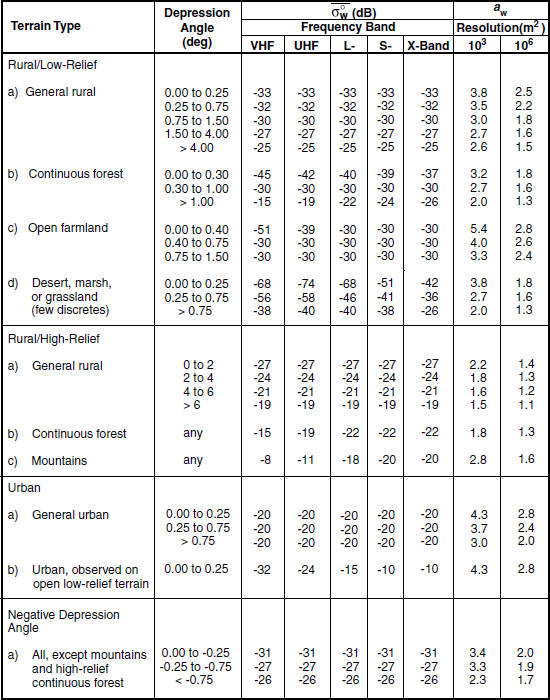
Second are parameters descriptive of the geometry of illumination of the clutter patch. As in Chapters 2 and 3, the interim model utilizes depression angle, a relatively simple and unambiguous quantity to determine, depending only on range and relative elevation difference between the radar antenna and the backscattering terrain point. Recall that attempts in Chapter 2 to use grazing angle met with little additional success, partly due to difficulties associated with scale, precision, and accuracy in unambiguously defining local terrain slope and partly because dominant clutter sources tend to be vertical discrete objects associated with the land cover. Use of grazing angle in clutter modeling is further discussed in Appendix 4.D. Formulating the interim clutter model in terms of depression angle involves the possibility of occurrence of negative depression angles wherein terrain is observed by the radar at elevations above the antenna. For terrain to be visible at negative depression angle requires the terrain to be of terrain slope greater than the absolute value of the depression angle at which it is observed.
Third are parameters descriptive of the terrain within the clutter patch. The interim clutter model of Table 4.2 is comprehensive in that, whatever terrain is under consideration, it must fall within one of the terrain types of the model. Most terrain types in the model involve several depression angle regimes. As introduced in Chapter 2, the important general terrain types of the interim model are threefold, namely (1) rural/low-relief terrain in which terrain slopes are < 2°; (2) rural/high-relief terrain in which terrain slopes are > 2°; and (3) urban terrain.
Within general rural/low-relief terrain, the interim model further distinguishes three specific important subclass terrain types as discussed in Chapter 3, namely, continuous forest, open farmland, and open wasteland (e.g., desert, marsh) or grazing land with very low incidence of large discrete vertical objects (e.g., farmstead buildings, feed storage silos, isolated trees, etc.) such as typically occur in farmland. Within rural/high-relief terrain, particularly separated out are the two subclass terrain types of continuous forest and mountains. Within urban terrain, separated out is the subclass of urban areas as observed over open low-relief terrain supportive of multipath (see Chapter 3). Concerning the several subcategories of terrain contained within each of the three general terrain types in Table 4.2, the general category (a) is applicable only if the terrain in question fails to meet the specification of any of the subsequent specific subcategories within a group. That is, the general category applies to mixed or composite terrain that is neither completely open nor completely tree-covered. The subcategorization of terrain within each major group becomes increasingly important with decreasing frequency. For completeness, a fourth general category comprising terrain observed at negative depression angle is required. Terrain observed at negative depression angle is usually relatively steep.
The interim clutter model of Table 4.2 consists of 27 combinations of terrain type and depression angle. For each combination, the model provides Weibull mean clutter strength as a function of radar frequency f, VHF through X-band, as ![]() , and provides the Weibull shape parameter as a function of radar spatial resolution A over the range between 103 and 106 m2, as aw(A). The shape parameter is obtained from linear interpolation on log10(A) between the values provided for A = 103 m2 and A = 106 m2. The total matrix of information in Table 4.2 contains all the important trends that are observed in the measured clutter amplitude distributions as discussed in Chapters 2 and 3.
, and provides the Weibull shape parameter as a function of radar spatial resolution A over the range between 103 and 106 m2, as aw(A). The shape parameter is obtained from linear interpolation on log10(A) between the values provided for A = 103 m2 and A = 106 m2. The total matrix of information in Table 4.2 contains all the important trends that are observed in the measured clutter amplitude distributions as discussed in Chapters 2 and 3.
Many of the important trends of variation in the ![]() data of Table 4.2 are plotted in Figure 4.4. These trends are now discussed in some detail. This discussion to some extent summarizes and reiterates previous discussions of the clutter measurement data in Chapters 2 and 3. Thus, in Figure 4.4, in general rural terrain of both low and high relief, mean clutter strength increases with depression angle but is invariant with frequency. That is, within the shaded region clutter strength rises with increasing depression angle both within the rural/low-relief and within the rural/high-relief regimes. In continuous forest, however, mean clutter strength depends both on depression angle and frequency; whereas in open farmland, mean clutter strength is invariant both with depression angle and frequency, except at low depression angle on level terrain where a significant multipath propagation loss occurs at low frequencies. Note that at intermediate depression angles in Figure 4.4, both forest and farmland fall in closely with general rural/low-relief terrain in terms of mean clutter strength.
data of Table 4.2 are plotted in Figure 4.4. These trends are now discussed in some detail. This discussion to some extent summarizes and reiterates previous discussions of the clutter measurement data in Chapters 2 and 3. Thus, in Figure 4.4, in general rural terrain of both low and high relief, mean clutter strength increases with depression angle but is invariant with frequency. That is, within the shaded region clutter strength rises with increasing depression angle both within the rural/low-relief and within the rural/high-relief regimes. In continuous forest, however, mean clutter strength depends both on depression angle and frequency; whereas in open farmland, mean clutter strength is invariant both with depression angle and frequency, except at low depression angle on level terrain where a significant multipath propagation loss occurs at low frequencies. Note that at intermediate depression angles in Figure 4.4, both forest and farmland fall in closely with general rural/low-relief terrain in terms of mean clutter strength.

Urban complexes observed over low-relief open terrain provide large mean clutter strengths at high frequencies partly because of their broadside aspect, but at low frequencies these large returns are decreased significantly through multipath loss. However, in more general composite terrain, mean clutter strength from urban complexes is 10 dB weaker than at high frequencies on open terrain and is frequency invariant.
On discrete-free desert, marsh, or grassland, mean clutter strength is weaker than for other terrain types. Again, at low and even intermediate depression angles, there is a large multipath loss due to decreased illumination strength at the lower frequencies, and this loss is greater and extends to higher frequencies than in farmland because the clutter sources are much lower in such terrain (e.g., a sagebrush bush) than in farmland (e.g., a silo). Note that, aside from differences in intrinsic σ°, propagation loss by itself would act to continue to decrease mean clutter strength ![]() from UHF to VHF at low and intermediate depression angles on open desert, marsh, or grassland; however, repeat sector data from four different sites and at all parametric variations of polarization and resolution show that mean clutter strength actually rises slightly from UHF to VHF, indicating that intrinsic σ° is considerably greater at VHF than UHF in such terrain.
from UHF to VHF at low and intermediate depression angles on open desert, marsh, or grassland; however, repeat sector data from four different sites and at all parametric variations of polarization and resolution show that mean clutter strength actually rises slightly from UHF to VHF, indicating that intrinsic σ° is considerably greater at VHF than UHF in such terrain.
Next mean clutter strength is compared between desert and forest at X-band. At low and intermediate depression angles, mean strength in desert terrain is 5 or 6 dB weaker than in forest terrain, but at high depression angle >1° (and on the basis of two different desert measurement sites at all combinations of polarization and resolution), mean strength in desert is equal to that in forest terrain (i.e., at X-band, looking down at sagebrush vegetation is equivalent to looking down at a forest canopy).
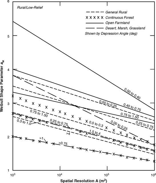
The data in Figure 4.4 cover 66 dB of variability in mean clutter strength, from mountains at VHF to desert at UHF. Of course, cell-to-cell variability in clutter amplitude statistics is even greater. The trends of variation in the aw data of Table 4.2 that determine cell-to-cell variability are shown in Figure 4.5 for rural/low-relief terrain. These results illustrate that spreads in clutter amplitude distributions due to cell-to-cell variability decrease both with decreasing spatial resolution and with increasing depression angle. Over and above these basic dependencies, the results in Figure 4.5 and Table 4.2 also show that aw in open farmland is greater than in general rural/low-relief terrain, whereas aw in continuous forest is less than in general rural/low-relief terrain; and that aw in rural/high-relief terrain is less than in rural/low-relief or urban terrain (see Figure 2.47).
4.2.3 ERROR BOUNDS
An interim multifrequency ground clutter model is provided in Table 4.2 for determining ground clutter amplitudes from visible regions of terrain in surface-sited radars. This interim model consists of a manageable set of empirically derived numbers that in total establishes an orderly rationale for the specification of such clutter amplitudes over their many order-of-magnitude range of variations, based on terrain type, depression angle, and the important radar parameters of frequency and resolution.
What are the error bounds in the interim modeling information presented in Table 4.2? The discussion of temporal and spatial variation in low-angle ground clutter previously provided in Section 3.7.3 provides some guidance in this matter. On the basis of repeat sector measurements over the two to three week stay at every Phase One site, the 1-σ diurnal variability in mean clutter strength, largely due to changes in weather, is specified in Section 3.7.3 to be 1.1 dB. The Phase One equipment made six repeated visits to selected sites to investigate seasonal variations. On the basis of these measurements, the 1-σ seasonal variability in mean clutter strength is specified in Section 3.7.3 to be 1.6 dB. Such long-term temporal variations in mean clutter strength from macroregions of terrain may be contrasted with the spatial region-to-region 1-σ variability that is specified in Section 3.7.3 to be 3.2 dB, on the basis of region-to-region variations in repeat sector mean clutter strength within similar regions. Thus, it is apparent that the numbers comprising the interim clutter model are statistical averages. These averages establish important trends, but actual realizations of clutter will deviate from the predicted average numbers of the model.
4.3 NON-ANGLE-SPECIFIC MODELING CONSIDERATIONS
In Section 4.2, the measured data were used to develop an interim clutter model for use in determining site-specific radar system performance, where the actual terrain at the radar site is deterministically represented through digitized terrain elevation data. Such a site-specific clutter model can provide, with reasonable fidelity, detailed measures of clutter-limited radar performance as a particular low-altitude airborne target is engaged by a particular radar at a particular site. At a higher level of abstraction, however, there remains a need for a non-patchy clutter model for use in computing the limiting effects of ground clutter on system performance in a generic sense, independent of how specific terrain features and resulting patchiness varies from site to site. This section brings the large database of Phase Zero ground clutter measurements statistically to bear to provide simple non-patchy clutter modeling information that captures the important statistical and parametric variations in the database. One important characteristic of a PPI clutter map is the obvious dissipation of the clutter with increasing range, which is automatically incorporated in a patchy site-specific model. Consideration of how best to implement this characteristic in a non-patchy non-site-specific model leads to discussion of explicit effects of range on low-angle clutter.
4.3.1 PHASE ZERO RESULTS
Figure 4.6 shows measured clutter maps to 47-km maximum range for six different sites, in order of increasing effective radar height. Figure 4.7 shows percent circumference in clutter vs range for the same six sites. The details of each pattern of spatial occurrence of clutter in Figure 4.6 are specific to the terrain features at that site. In all such patterns, however, the patches of clutter become fewer and farther between with increasing range so that, as shown in Figure 4.7, the amount of clutter that occurs gradually diminishes with increasing range from the site. These two figures also show that the amount of clutter that occurs is a strong function of the effective height of the radar. Effective radar height is defined with respect to visible terrain and includes both the height of the hill on which the radar is situated and the antenna mast height (see Section 2.2.3). The somewhat differing higher-order effects of hill height and mast height on terrain visibility are discussed in Appendix 4.B. It is apparent in Figures 4.6 and 4.7 that higher radars see clutter to longer ranges.
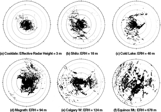
FIGURE 4.6 Phase Zero clutter maps for six sites. In each map, maximum range = 47 km (10-km range rings). Results shown are for full Phase Zero sensitivity.

FIGURE 4.7 Percent circumference in clutter vs range for six sites. Phase Zero data, 47-km maximum range, 150-m range resolution, clutter threshold is 3 dB above full sensitivity.
Figure 4.8 provides general information on clutter extent and strength by averaging measurements like those of Figures 4.6 and 4.7 from many sites. Figure 4.8(a) shows percent of circumference in clutter vs range averaged across 86 sites. The resultant clutter visibility curve is approximately linear over most of its extent as displayed on the logarithmic vertical scale employed in Figure 4.8(a). This linearity indicates that in general the amount of ground clutter that occurs in surface radar decreases exponentially with increasing range, thus quantifying the observations of the preceding paragraph. The curve of Figure 4.8(a) represents the best non-site-specific information that the large Phase Zero database can deliver when brought to bear to answer the general question, how far out does ground clutter go? Because ground clutter diminishes gradually (i.e., exponentially) with increasing range, this question must be answered conditionally in terms of a threshold on how much clutter is of concern. As an example, Figure 4.8(a) indicates that in general 10% of circumference is in clutter at 19-km range.

FIGURE 4.8 General spatial extent and strength of low-angle radar ground clutter: (a) decrease of clutter occurrence with range and (b) distribution of mean strengths of ground clutter patches.
Percent circumference in clutter represents the probability of discernible clutter Pc vs range r. Pc(r) is dependent on radar sensitivity. If it is assumed that clutter arises only from geometrically visible terrain and that over visible terrain clutter is Weibull-distributed, then it is straightforward to numerically extrapolate the Phase Zero clutter visibility data of Figure 4.8 to radars of higher sensitivity. In this extrapolation, Pc(r) = Pv(r)·PD(r), where Pv(r) is the probability that the terrain is geometrically visible, and PD(r) is the probability that the clutter strength is above radar noise level given that the terrain is visible. PD(r) is simply the Weibull cumulative (integral) distribution function obtained by integrating Eq. (2.B.18) with radar noise level at range r as the lower limit of integration [(cf. Eq. (2.B.21) obtained with zero as the lower limit of integration]. PD(r) is easily numerically evaluated, once the Weibull coefficients of the clutter and the noise level of the radar are specified. If the ratio of PD(r) for a radar of increased sensitivity to PD(r) for Phase Zero sensitivity is computed, then clutter visibility Pc(r) for the radar of increased sensitivity is simply the product of this ratio and Pc(r) for Phase Zero as given by the data in Figure 4.8. The validity of such extrapolation of Phase Zero clutter visibility data to higher sensitivity radars is dependent on the soundness of the assumptions, which deteriorate with large departure from Phase Zero sensitivity.
Discussion now turns to Phase Zero clutter amplitude distributions as obtained within macropatches of visible terrain. Figure 4.8(b) shows the cumulative distribution of mean clutter strengths, one mean value per clutter patch, over all the 2,177 patches for which Phase Zero clutter amplitude distributions were determined. These 2,177 macropatches were selected from 96 different measurement sites. The curve of Figure 4.8(b), as plotted on a logarithmic (i.e., decibel) abscissa, is essentially linear over most of its central extent.
This linearity implies that the distribution of mean strengths of clutter patches (in units of m2/m2) is lognormal. The data in Figure 4.8(b) represent Phase Zero’s best answer to the next general question, how strong is ground clutter? Figure 4.8(b) indicates that mean ground clutter strength varies over five orders of magnitude. Thus this question also must be answered conditionally in terms of probability of occurrence. The median or 50-percentile value of mean clutter strength in this figure is −31 dB (i.e., half of all measured values of mean clutter strength occur above −31 dB, half below). The mode or most frequently occurring value of mean clutter strength in Figure 4.8(b) is −40 dB.
4.3.2 SIMPLE CLUTTER MODEL
In developing a simple non-site-specific clutter model, the first issue that must be confronted is terrain visibility. As previously discussed, from most places on the surface of the real earth, visibility to terrain is spatially patchy. To an observer looking out from the site, high regions are visible and intervening low regions are masked. Most of the relatively significant clutter comes from directly (geometrically) visible terrain. As range increases, the visible terrain patches become fewer and farther between until beyond some maximum range, no more terrain is visible. Thus on the real earth, terrain visibility and hence the spatial occurrence of clutter is a gradually diminishing function of increasing range.
Here, a simple non-site-specific clutter model means a non-patchy model that is spatially homogeneous and isotropic. The sort of earth that provides this kind of clutter is a cue ball earth. That is, if the site-specific macroscopic terrain features that exist at every real site are suppressed, what remains is a cue ball, conceptually devoid of all macrofeature, but uniformly microrough to account for homogeneous and isotropic diffuse clutter backscatter. On such a cue ball devoid of macroscale terrain features, the clutter patches observed at real sites expand to encompass all of the terrain out to a single-valued horizon, RC. The resulting binary visibility function is imparted to the simple clutter model. There may be a temptation to spatially dilute the clutter amplitude statistics as actually measured within large macropatches of visibility with the large amounts of macroshadow that exist on the real earth between the patches. Such spatial dilution would artificially diminish clutter strengths with increasing range in a way that would certainly not be measured by a real radar, either on a real earth-sized cue ball or on the real earth itself. These matters are discussed at greater length in Appendix 4.C.
Such considerations lead to the simple, non-patchy, non-site-specific clutter model shown in Figure 4.9. This simple model provides homogeneous clutter within a circular region centered at the radar. The mean clutter strength within this region is given by ![]() , and the radial extent of the region by the clutter cut-off range RC. The statistically important effect of increasing macroshadow with increasing range shown in Figure 4.8(a) is used to set the radial extent of the homogeneous clutter region RC. This setting of RC is done as a statistical threshold on clutter visibility in the measured data. That is, the user first specifies the minimum spatial amount of clutter that begins to degrade the user’s systems (e.g., 20%). Then the range at which that amount of clutter generally occurs in the measurements is used as the clutter cut-off range RC in the simple model (e.g., 12 km).
, and the radial extent of the region by the clutter cut-off range RC. The statistically important effect of increasing macroshadow with increasing range shown in Figure 4.8(a) is used to set the radial extent of the homogeneous clutter region RC. This setting of RC is done as a statistical threshold on clutter visibility in the measured data. That is, the user first specifies the minimum spatial amount of clutter that begins to degrade the user’s systems (e.g., 20%). Then the range at which that amount of clutter generally occurs in the measurements is used as the clutter cut-off range RC in the simple model (e.g., 12 km).

The effective height of the radar above the surrounding terrain is the major parameter affecting how far ground clutter occurs. This effect is illustrated by the data of Figure 4.10, in which the exponential decrease of clutter occurrence with increasing range shown in Figure 4.8(a) is parameterized in five regimes of effective radar height, using the same 86-site set of data upon which the result of Figure 4.8(a) is based. Figure 4.10 may be compared with Figure 4.7. Again, it is apparent that higher radars see clutter to longer ranges. The simple model incorporates this important effect of radar height by parameterizing the statistical procedures for setting clutter cut-off range to be dependent on radar height in the measured data.
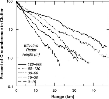
The results of these procedures for specifying clutter cut-off range RC in the non-site-specific model are summarized in Table 4.3. If 20% of circumference in clutter on the real earth is accepted as a baseline threshold above which clutter is expected to have substantial impact on radar system performance, Table 4.3 indicates that at a general radar height of 40 m, this threshold in clutter occurrence will be exceeded at ranges ≤ 12 km. If it is known that the radar is substantially lower or higher than this general height of 40 m, the clutter cutoff range decreases to 7 km or increases to 22 km, respectively, for the same baseline threshold in clutter occurrence. If the threshold in clutter occurrence rises to as much as 50%, clutter extents above such a high threshold are relatively benign, 3 or 4 km, whereas if the threshold in clutter occurrence drops to as little as 2%, clutter extents are quite severe, ranging from 21 to 48 km depending on radar height. Note that except for this latter severe situation, clutter extents as derived empirically in Table 4.3 from clutter visibility on the real earth are usually much less than range to the spherical earth horizon on a cue ball, illustrating that on the real earth, terrain relief usually dominates over earth sphericity in influencing terrain visibility and horizons.

With the radial extent of the homogeneous region determined in this manner for the simple model, the mean strength of the clutter ![]() that exists within this region must be specified.
that exists within this region must be specified.
To do so, mean clutter strengths as measured over many macropatches in the measured data are used as illustrated by the data of Figures 2.23, 2.24, 2.35, and 4.8(b). Table 4.4 provides a resulting matrix of information showing how mean clutter strength varies with terrain type and probability of occurrence. If the 50-percentile level is accepted as a baseline probability of occurrence, then in completely general or non-terrain-specific circumstances the data suggest ![]() dB as the best single measure of mean clutter strength. However, if it is known that the terrain is either relatively low or high relief or urban, mean clutter strength
dB as the best single measure of mean clutter strength. However, if it is known that the terrain is either relatively low or high relief or urban, mean clutter strength ![]() may be adjusted to −33, −27, or −23 dB, respectively, at the same 50-percentile probability of occurrence. Proceeding to a worst-case/best-case assessment, if 90- and 10-percentile probabilities of occurrence are accepted as reasonable measures of strong and weak mean clutter strengths, respectively, then by these measures the data in Table 4.4 show that strong mean clutter strength is generally 7 or 8 dB stronger than baseline, and weak clutter is generally 7 or 8 dB weaker than baseline, both in general circumstances and for the three main terrain types.
may be adjusted to −33, −27, or −23 dB, respectively, at the same 50-percentile probability of occurrence. Proceeding to a worst-case/best-case assessment, if 90- and 10-percentile probabilities of occurrence are accepted as reasonable measures of strong and weak mean clutter strengths, respectively, then by these measures the data in Table 4.4 show that strong mean clutter strength is generally 7 or 8 dB stronger than baseline, and weak clutter is generally 7 or 8 dB weaker than baseline, both in general circumstances and for the three main terrain types.

4.3.3 FURTHER CONSIDERATIONS
4.3.3.1 Clutter Strength vs Range
Ground clutter strength depends principally on the depression angle at which the backscattering terrain point is illuminated as it varies with terrain elevation from point to point over a site. The simple, non-patchy, non-site-specific clutter model does not incorporate local variability in terrain elevation and hence would be able to bring in depression angle only as a very slowly diminishing function with increasing range on a spherical earth. Is this small rate of change of illumination angle with range sufficient to cause an observable general dependence of clutter strength with range in measured data?
To begin to answer this question, consider again the measured clutter maps of Figure 4.6. These measurements are shown at full Phase Zero sensitivity. When the clutter in the maps is shown only above a gradually increasing threshold in clutter strength, except at very close ranges the density of the clutter sources within patches gradually diminishes relatively uniformly over the remainder of the map at longer ranges, indicating that within patches of visibility, clutter strength is relatively independent of range beyond the first few kilometers (e.g., see Figure 4.19). That is, the clutter does not disappear at the longer ranges first. Sector display plots of clutter amplitude vs range such as are shown in Figures 2.10, 2.18, 2.20, and 3.11 also do not indicate any general diminishment of clutter strength with range through patches of clutter occurrence. This matter is discussed further in Appendix 4.A, in which similar sector display plots are shown to much longer ranges.
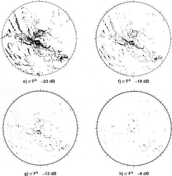
FIGURE 4.19(E-H) Thresholded PPI clutter plots at Cochrane, Alta. Phase Zero X-band data. Maximum range = 24 km; range resolution = 75 m. North is at zenith.
Results generalizing the lack of range dependency in clutter are provided in Figure 4.11. Clutter amplitude statistics combined from 10 different sites are separated into four annular regimes of range—from 5 to 15 km, 15 to 25 km, 25 to 35 km, and 35 to 45 km. Care must be taken to properly normalize the results. First, because the amount of clutter rapidly diminishes with increasing range, only those cells in which discernible clutter are measured above the radar noise floor are included. Second, because radar sensitivity diminishes with increasing range, the results are normalized to range-independent sensitivity by further conditionally limiting included cells to only those in which clutter signals are stronger than system noise at the longest ranges, that is σ°F4 > −24 dB. The results of Figure 4.11 indicate that there is essentially no dependence with range in the resulting clutter amplitude statistics. These results are discussed further in Appendix 4.C.
Because clutter strength shows no major dependence upon range, ![]() in the simple non-patchy model abruptly transitions from a constant nonzero m2/m2 value within RC to zero m2/m2 beyond RC. This abrupt transition keeps before the user the simple non-site-specific nature that was initially postulated as a requirement of the model in the results of system studies implementing the model. When step function performance characteristics are unacceptable, it is not realistic to arbitrarily decrease clutter strength
in the simple non-patchy model abruptly transitions from a constant nonzero m2/m2 value within RC to zero m2/m2 beyond RC. This abrupt transition keeps before the user the simple non-site-specific nature that was initially postulated as a requirement of the model in the results of system studies implementing the model. When step function performance characteristics are unacceptable, it is not realistic to arbitrarily decrease clutter strength ![]() with increasing range in the simple model to introduce more acceptable, continuous characteristics with range and avoid step function characteristics. In reality, it is the spatial occurrence of clutter, not its strength, that diminishes with range.
with increasing range in the simple model to introduce more acceptable, continuous characteristics with range and avoid step function characteristics. In reality, it is the spatial occurrence of clutter, not its strength, that diminishes with range.
It is certainly incorrect to simply multiply the clutter strength by the visibility function to provide what may be thought to be a more desirable modeling characteristic of diminishing clutter strength with increasing range. Such a procedure involving azimuthal averaging (i.e., spatial dilution of clutter with macroshadow) is only applicable to an unrealistic radar with a 360° omnidirectional azimuth beam [in such circumstances, it is the shadowless mean that is multiplied by the visibility function; see Appendix 4.C for further discussion of this matter, in particular, Eq. (4.C.4) and Figures 4.C.16 and 4.C.17)].

FIGURE 4.C.16 Mean levels (upper bound, lower bound, and shadowless) of ground clutter strength vs range, averaged omnidirectionally over 10 sites. Phase Zero X-band data, horizontal polarization, 150-m range resolution, 0.9° azimuth beamwidth. Range sampling interval = 148.4 m, azimuth sampling interval = 0.2344°, 1,536 azimuth samples/range gate/site.

FIGURE 4.C.17 Fraction of circumference in clutter vs range, averaged omnidirectionally over 10 sites. Phase Zero X-band data, horizontal polarization, 150-m range resolution, 0.9° azimuth beamwidth. Range sampling interval = 148.4 m, azimuth sampling interval = 0.2344°, 1,536 azimuth samples/range gate/site.
Thus when step function performance characteristics are unacceptable, a more sophisticated clutter model incorporating a gradually diminishing clutter occurrence or visibility function must be employed. The site-specific clutter model discussed in Section 4.2 incorporates gradually diminishing terrain visibility with increasing range as determined by line-of-sight geometric terrain visibility in DTED. In addition, a patchy non-site-specific clutter model was developed [3] by the Defence Evaluation and Research Agency/U.K. which conducted analyses of some subsets of Phase One clutter data coordinated with Lincoln Laboratory. The patchy non-site-specific clutter model was based on the empirically observed exponential decrease of clutter visibility with range as shown in Figures 4.8(a) and 4.10 to provide stochastic realizations of random patchiness representative of a particular type of terrain, as opposed to deterministic site-specific realizations of patchiness. In the stochastic approach to patchiness, the characteristics of the terrain that determine the patchiness are obtained by processing DTED over the general terrain of interest. Such stochastic techniques for providing non-site-specific patchiness in a clutter model are more appropriate for low-relief terrain, as high-relief terrain is too specific in terms of dominant terrain features within the radar coverage area to be properly characterized as a random process.
4.3.3.2 SPREAD IN CLUTTER AMPLITUDE STATISTICS
Ground clutter amplitude distributions have wide spread resulting from cell-to-cell spatial variation within macropatches of clutter occurrence. This wide spread is illustrated by the data in Figure 4.12, which show percentile levels between 50 and 90 in ground clutter amplitude distributions both for general terrain and for the three primary terrain types. Each percentile value plotted in Figure 4.12 is the median of the set of corresponding individual percentiles from all clutter patches of that class within the overall set of 2,177 clutter patch amplitude distributions. Figure 4.12 typically shows about 16 dB of variation between 50- and 90-percentile levels. Furthermore, this figure also shows that the mean value, indicated by a vertical arrow, is usually close to the 90-percentile level (except for rural/high-relief terrain in which illumination angles are higher and hence the influence of discrete sources, which tend to dominate the mean, are reduced).

Should a percentile level lower than the mean be used in selecting a value for σ°w in the simple model? This question has no simple answer. The data displayed in Figure 4.12 illustrate the conceptual difficulty of modeling a widely varying dynamic random process with a single deterministic number. However, some guidance may be offered toward answering this question. In a system study simulating the existence of low-altitude targets at a number of Phase One clutter measurement sites, the resultant radar performance, averaged over all sites, was approximately the same as would be computed if a constant clutter strength of σ°w = −38 dB was used over all visible terrain. This value of clutter strength occurs at the 70-percentile level on the general terrain curve of Figure 4.12, approximately halfway between the mean and the median. Recall that the most probable value of mean clutter strength in the general data of Figure 4.8(b) is −40 dB, perhaps a fortuitous concurrence. The reader is cautioned that this is a particular result of only one study and that such values of constant-σ° that provide equivalent system performance as real clutter (or site-specifically simulated clutter) are highly specific to the particular radar system and performance parameters under consideration. In any case, the data of Figure 4.12 allow investigators to adjust modeling values of σ°w away from the mean values shown in Table 4.4, if they so desire.
4.3.3.3 DATABASE DEPTH
The easy-to-use data for RC and ![]() in Tables 4.3 and 4.4 capture the most important first-level effects contained in the large database of measurements for simple non-site-specific modeling applications. Consideration of higher-order effects can provide ever-increasing specificity of information. For example, consider the distributions of mean strength in six classes of landform and land cover provided earlier in Figures 2.23 and 2.24, respectively. One can imagine similar distributions by landform and land cover for median strength or for other statistical measures of the patch amplitude distributions. The data in Tables 4.5 and 4.6 provide quantitative measures of distributions of means, ratios of standard deviation-to-mean, medians, and various percentile levels, by landform and land cover, respectively. Thus the data of Tables 4.5 and 4.6 may be drawn upon to expand the simplified information of Table 4.4 to other probabilities of occurrence, other measures of strength (e.g., median), and other landform and land cover types
in Tables 4.3 and 4.4 capture the most important first-level effects contained in the large database of measurements for simple non-site-specific modeling applications. Consideration of higher-order effects can provide ever-increasing specificity of information. For example, consider the distributions of mean strength in six classes of landform and land cover provided earlier in Figures 2.23 and 2.24, respectively. One can imagine similar distributions by landform and land cover for median strength or for other statistical measures of the patch amplitude distributions. The data in Tables 4.5 and 4.6 provide quantitative measures of distributions of means, ratios of standard deviation-to-mean, medians, and various percentile levels, by landform and land cover, respectively. Thus the data of Tables 4.5 and 4.6 may be drawn upon to expand the simplified information of Table 4.4 to other probabilities of occurrence, other measures of strength (e.g., median), and other landform and land cover types
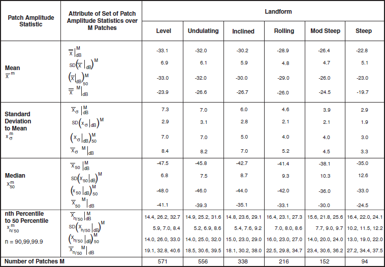
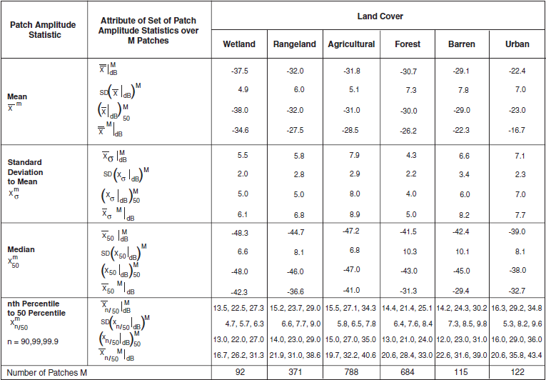
The statistical attributes shown in the second column of Tables 4.5 and 4.6 are now defined more explicitly. Observe in Figures 2.23 and 2.24 that the distributions are approximately lognormal. As a result, it is useful to define the mean and standard deviation of the normally distributed logarithmic quantity. These two quantities are shown as the first (i.e., top-most) and second attributes for each patch amplitude statistic. The third attribute shown is the median, which itself just transforms logarithmically. If the logarithmic quantity is normally and hence symmetrically distributed, its mean and median must be identical. The data in Tables 4.5 and 4.6 indicate that these two quantities (i.e., the first and third attributes, respectively) are, indeed, often nearly equal. Once it is assumed that the distribution is approximately lognormal, all other attributes of the distributions of both the logarithmic quantity and the more fundamental underlying linear quantity immediately follow from the first and second attributes provided in Tables 4.5 and 4.6. However, the fourth and final attribute for each patch amplitude statistic shown is the actual empirical mean of the basic linear quantity, which can be used either directly in its own right or as a further check on the degree of goodness of the approximating lognormal distributions.
Now consider some of the trends with landform contained in the data of Table 4.5, where terrain slopes rise monotonically with landform class, left to right, from less than 1° for level terrain to between 10° and 35° for steep terrain (see Figure 2.23). Consider the median of M samples within a particular landform class of a given statistic (e.g., mean) of a clutter amplitude distribution as an easy-to-understand attribute, in that half the samples occur above the median level and half below. The median attribute is shown in increasing order of landform as the third row of numbers for each patch amplitude statistic in Table 4.5. Thus, as terrain slopes rise from level to steep, the third rows of the table show that (1) mean strengths rise over the 10-dB range from −33 to −23 dB; (2) median strengths rise over the 15-dB range from −48 to −33 dB; (3) spreads in amplitude distributions as measured by ratio of standard deviation-to-mean fall from 7 to 3 dB, spreads as measured by ratio of 99.9- to 50-percentile fall from 33 to 22 dB, and spreads as measured by ratio of mean-to-median fall from 15 to 10 dB. All the trends are monotonic with increasing terrain steepness as specified by the median value from a large number M of individual patch measurements within each landform class.
In considering increasing specificity of information, recall that all the non-site-specific information presented in this section has been derived from X-band measurements. However, when considering that mean strengths from the three general terrain types of rural/low-relief, rural/high-relief, and urban are largely frequency independent, and that the simple model is already averaging out much fine-scaled variation, it is not unrealistic to apply the simple model across the general microwave regime. Investigators who wish to introduce more specific frequency dependence in non-site-specific investigation may, as a beginning, be guided by the multifrequency mean data of Table 4.2.
4.3.4 SUMMARY
The considerations guiding the development of the simple, non-angle-specific clutter modeling information presented in Section 4.3 are now summarized. The objective is to invest a simple clutter model with important general attributes as they have come to be understood in investigating the large database of clutter measurements. Of first-order importance is to distinguish between where the clutter occurs and its strength, given that it occurs. The simple, non-patchy model of Section 4.3.2 maintains this distinction by first specifying clutter cut-off range based on the measurements of clutter visibility, and then specifying clutter strength based on measurements of clutter amplitude statistics within macropatches of occurrence. Furthermore, this model brings in the important parameters of radar height as it influences clutter extent and terrain type as it influences clutter strength. In this empirical manner, the model maintains its focus on the important first-level parameters in the real clutter phenomenon and statistically provides baseline central values of clutter strength and extent as they occur at real sites.
The simple model does more than this, however. In addition to providing central measures, the model also specifies the distributions. As a result, besides providing information on baseline values of strength and extent of clutter, the model also provides parametric information on how severe (i.e., strong clutter to long-range) or how benign (i.e., weak clutter to short-range) the clutter can become, all in terms of specifiable probability of occurrence. It is this depth of statistical information in the simple model incorporating the extreme variability of the clutter phenomenon in quantitative terms of probability of occurrence, more so than the baseline central values of the model, that sets it apart from other single-point approaches in the literature.
4.4 TERRAIN VISIBILITY AND CLUTTER OCCURRENCE
Figure 4.10 in Section 4.3.2 shows percent of circumference in discernible clutter as a function of range for five regimes of effective radar height, as measured by the Phase Zero radar with a mast height of 15 m. These clutter occurrence curves of Figure 4.10 may be compared with those of Figure 4.B.3 (in Appendix 4.B) which show percent of circumference over which terrain is visible, also from a mast height of 15 m and as a function of range, for four regimes of site advantage. The occurrence of clutter (Figure 4.10) is strongly tied to line-of-sight visibility to terrain (Figure 4.B.3). That is, clutter occurs primarily within visible terrain macroregions in which discrete clutter sources are separated by randomly occurring microshadowed cells where the radar is at its noise level. Because of the microshadowing that occurs within macroregions of general visibility, the spatial extent of terrain visibility is greater than, and can be much greater than, the spatial extent of discernible clutter, as is apparent in comparing the curves of Figure 4.B.3 with those of Figure 4.10.

FIGURE 4.B.3 Mean terrain visibility vs range for four regimes of site advantage, with a 15-m antenna mast height. Based on bare-earth DTED for 43 hilltop sites.
Figure 4.13 shows the same terrain characterized by DTED obtained from two different sources, cartographic (maps) and photogrammetric (aerial photos). It is evident that photogrammetric source DTED are more precise and provide fine-scale terrain detail not contained in the cartographic source DTED. The cartographic source DTED capture the basic first-order characteristics of the terrain land-surface form, and are highly suitable for distinguishing macroregions of visible terrain from macroregions of shadow. The increased precision of photogrammetric source DTED may begin to allow deterministic prediction of microshadowed cells within macroregions of visibility. However, land cover elements are much more involved as the predominant sources of microshadow, as is seen in the following Cold Lake results.

FIGURE 4.13 Three-dimensional oblique views of the same terrain characterized by digitized terrain elevation data derived from two sources: (a) maps and (b) aerial photos. The terrain shown is a common 30 km × 30 km test area.
4.4.1 EFFECTS OF TREES ON VISIBILITY AT COLD LAKE
Trees are often dominant components of land cover affecting low-angle clutter (see Chapter 2, Section 2.4.2.5). Figure 4.14 shows the dramatic effect on clutter visibility of predicting tree heights in individual spatial cells at the measurement site of Cold Lake, Alberta. These results incorporate cell-specific tree cover information derived from Landsat data to obtain a more precise and accurate clutter map prediction.

FIGURE 4.14 Effects of tree heights on ground clutter visibility at Cold Lake, Alta. The maximum range in each plot is 23.5 km. (a) terrain elevation contour plot, 20-m intervals; (b) geometric visibility to ground (black), no trees; (c) Phase Zero ground clutter measurement, σ°F4 ≥−30 dB, 75-m range resolution; (d) geometric visibility to ground (black), with Landsat trees.
Figure 4.14(a) shows terrain elevation contour plots at 20-m intervals at Cold Lake, obtained from cartographic source DTED which does not include tree heights. In the northeast quadrant of this plot, the large level surface at 540-m elevation is water, the surface of Cold Lake. Four small islands are visible in the southern part of the lake. Figure 4.14(b) shows geometric visibility to bare ground (or water) based on these DTED. In Figure 4.14(b), visible areas of the ground are shown as black, and masked or shadowed areas of the ground are shown as white. Large continuous regions of the ground, including much of the surface of Cold Lake itself, are indicated as being within line-of-sight visibility in Figure 4.14(b). Figure 4.14(c) shows the Phase Zero ground clutter measurement at Cold Lake. The Cold Lake area in north-central Alberta is generally forested, although considerable regions have been cleared for farming. Within the large continuous black macroregions of visibility of Figure 4.14(b), actual clutter sources of σ°F4 ≥−30 dB occur as black micropatches in Figure 4.14(c), interspersed with a considerable degree of white microshadowing.
Figure 4.14(d) shows how geometric visibility to the ground is modified by cell-specific inclusion of the occurrence of trees on the landscape. Landsat data for the Cold Lake area were classified in a scheme that included deciduous and coniferous tree categories. These data were registered with the terrain elevation data at Cold Lake. Each DTED cell that Landsat indicated as containing trees was increased in effective masking elevation by a statistical increment to account for the tree heights. A Gaussian statistical tree height increment was used such that: (1) mean height = 20 m, standard deviation = 0.9 m, for deciduous classification; and (2) mean height = 25 m, standard deviation = 1.8 m, for coniferous classification.
Including the effects of tree heights on terrain visibility in Figure 4.14(d) in this way greatly changes the character of the bare ground visibility map of Figure 4.14(b), mainly by introducing cell-specific microshadowing effects within large macroregions of visibility. The bare-earth model at Cold Lake [Figure 4.14(b)] shows much higher terrain visibility than when trees are accounted for [Figure 4.14(d)]. Much of the water surface of Cold Lake itself, indicated as visible without trees in Figure 4.14(b), becomes shadowed when trees are included in Figure 4.14(d). Whether shadowed or not, the water surface of Cold Lake is below the clutter strength threshold in Figure 4.14(c) and is indicated as white there. Thus, careful incorporation of site-specific and cell-specific variations in elevation, for example, due to trees, can account for much detailed feature in a measured ground clutter map, based on geometric visibility considerations alone without any recourse to propagation or scattering physics.
4.4.2 DECREASING SHADOWING WITH INCREASING SITE HEIGHT
Although there exists much correlation in terms of general features between the measured Cold Lake clutter map of Figure 4.14(c) and the predicted map inclusive of tree height effects of Figure 4.14(d), careful examination indicates that on a more detailed cell-by-cell basis the correlation in these maps deteriorates. Successful reduction of clutter measurement data in a cell-specific manner in which measured clutter strength in a cell is associated with cell-specific geometric effects such as tree height and grazing angle would require terrain descriptive Geographic Information System (GIS) data of very high precision and accuracy.
The reduction of measured clutter data as described in this book uses available DTED more simply to predict boundaries of macroregions of general terrain visibility, which are denoted as clutter patches. Then all of the measured clutter data within the boundaries of the specified patch, including cells at radar noise level, are assembled in a histogram of clutter strengths associated with the patch. Figure 4.15 shows six such measured histograms, one for each of six different sites (including Cold Lake) in order of increasing effective radar height. In these histograms, the 50-, 90-, and 99-percentile levels are shown as vertical dotted lines; the mean strength is shown as a vertical dashed line; and bins to the left side of the histogram that are significantly contaminated by radar noise samples are doubly underlined. Figure 4.16 shows the cumulative distributions above the highest noise contaminated bin for each of these six patches. Table 4.7 shows the incidence of microshadowing within each patch and its effect on the mean clutter strength of the patch. For example, the incidence of microshadowing for the Cold Lake patch for which the clutter strength histogram is shown in Figure 4.15(c) is 35%.
TABLE 4.7
Influence of Effective Radar Height on Incidence of Microshadowing for Six Clutter Patches
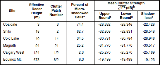
aMicroshadowed cells are defined to be cells within patches at radar noise level.
bComputed in units of m2 /m2 and subsequently converted to dB.
cAssign noise power level to noise cells.
dAssign zero power level to noise cells.
eNoise cells deleted.

FIGURE 4.15 Clutter strength histograms for six patches selected from sites in different regimes of effective radar height. Phase Zero data, 75-m range resolution.
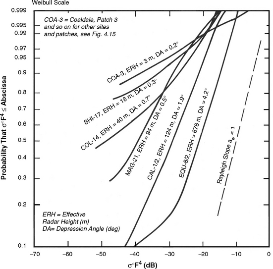
FIGURE 4.16 Six clutter patch cumulative amplitude distributions from sites in different regimes of effective radar height. Phase Zero data, 75-m range resolution.
It is evident in these results that the incidence of microshadowing within clutter patches decreases rapidly with increasing effective radar height. At low sites such as Coaldale and Shilo, the incidence of microshadowing can be very high (74% at Coaldale), but even so the mean clutter strength of the patch as determined within the upper- and lower-bound limits remains accurate (to within 0.014 dB at Coaldale). The mean strength of the patch determined in this manner includes the effects of microshadowing and is accurate independent of the sensitivity of the measurement radar; so also is the cumulative distribution for the patch (above the highest noise contaminated bin) as is shown in Figure 4.16 and from which the Weibull shape parameter aw is obtained. The shadowless mean clutter data shown in Table 4.7 which do not include samples within the histogram at radar noise level are highly dependent on the particular sensitivity of the measurement radar utilized and are not generally useful in clutter modeling (although such data are often inappropriately used in the existing clutter literature).
4.4.3 VERTICAL OBJECTS ON LEVEL TERRAIN AT ALTONA
Prediction of clutter strengths based on the information provided in this book proceeds on the basis of many measured patch histograms and cumulative distributions of clutter strength such as are shown in Figures 4.15 and 4.16. Given the occurrence of a visible terrain macroregion, the subsequent distribution of modeled clutter over the region is specified as a broad Weibull distribution of appropriate shape parameter aw that includes the distribution of microshadowed cells at the correct incidence of occurrence as Weibull values below the noise level of the radar under investigation. Not only is the prediction of patch mean strength independent of radar sensitivity, but the incidence of microshadowing that is predicted is appropriate to the sensitivity of the radar under investigation, which can be different from that of the measurement radar. The predicted microshadowed cells within the patch for which clutter is being predicted occur randomly within the patch. Prediction of clutter in this manner thus proceeds accurately without being dependent on the availability of highly precise and accurate cell-specific GIS terrain descriptive data.
For low-relief sites at short ranges where terrain visibility is very high (e.g., Figure 4.B.3, range < 10 km, site advantage regime = 10 to 35 m), visibility of discernible clutter is very low (e.g., Figure 4.10, range < 10 km, effective radar height = 0 to 30 m). The reason for this can be seen in the PPI clutter map for Altona II shown in Figure 4.17. The terrain at Altona II is very level cropland, much like that at Coaldale [see Figure 4.15(a)]. From the 15-m Phase Zero antenna mast height, virtually all of the terrain within the 6-km maximum range clutter map of Figure 4.17 is predicted as visible using bare-earth DTED to model the Altona II terrain surfaces. Yet only within the nearest 1 or 2 km is the Phase Zero radar generally sensitive to the backscatter from these terrain surfaces. The several white sectors within the central black region are due to local masking by clusters of trees near the radar site. At longer ranges, it is the vertical objects on the terrain associated with the land cover that constitute strong backscatter sources. Many of these are associated with individual farmsteads and trees around farmsteads, although roads, rail lines, power line pylons, and stream beds are also sources of discernible clutter. The predominant rectangular pattern is associated with vertical objects along field boundaries. The reason backscatter from the field surfaces, as opposed to that from vertical objects on the fields, is weak and generally below the sensitivity of the measurement radar is partly because the illumination occurring beyond 1 or 2 km is very close to grazing incidence and partly because many of these low surfaces are shadowed by land cover features not included in DTED (e.g., road and rail beds) that are a few feet higher than the field surfaces proper.
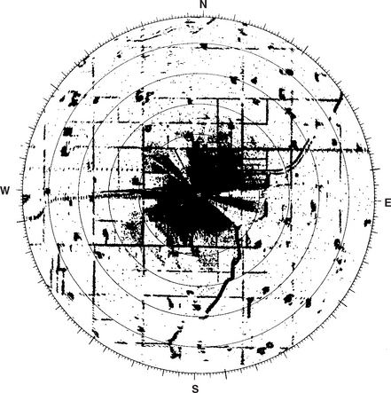
FIGURE 4.17 High resolution clutter map at Altona II, Manitoba. Phase Zero X-band data, 6-km maximum range setting, 9-m range resolution. The clutter map is 3 dB from full sensitivity. Clutter is black. North is zenith.
Thus, all of the terrain in Figure 4.17 is within geometric line-of-sight visibility as modeled with DTED, yet the clutter sources are predominantly vertical objects associated with land cover as they exist distributed over this nominally visible terrain. As a result, the extent of discernible clutter (black) in Figure 4.17 is much less than the extent of nominally visible terrain, and a very high incidence of white microshadowed cells occurs between the black clutter cells.
4.4.4 SUMMARY
Determination of geometric terrain visibility in a bare-earth faceted terrain model based on DTED predicts general terrain regions in which clutter sources occur. Predicting the existence of clutter thus arises from a set of conditional probabilities, in which the first and most important condition for the existence of clutter at some spatial position is for that position to be geometrically visible. Consider again (see Section 4.3.1) that the probability of discernible clutter Pc is given by the probability that the terrain is geometrically visible Pv times the probability PD that the clutter strength is discernible, given that the terrain is visible. As discussed in Section 4.3.1, PD is easily numerically evaluated, once the Weibull coefficients of the clutter and the noise level of the radar are specified.
Further conditions on clutter discernibility, in addition to the radar sensitivity at the point under consideration, are those associated with land cover, as discussed for Altona II and Cold Lake, or conditions associated with propagation. For example, as discussed in Chapter 3, at low radar frequencies such as VHF, little clutter may be received from low-relief terrain because terrain reflections prevent illumination of the terrain, even though it is within line-of-sight. Or some VHF clutter may be received from regions somewhat beyond geometric visibility due to diffraction, if the radar sensitivity is high enough to discern relatively weak clutter (clutter strength for shadowed terrain depends on depth of shadow; see Appendix 4.D). The Phase One clutter data indicate that determination of bare-earth terrain visibility is the most useful first step in understanding the spatial occurrence of ground clutter, even at VHF. Effective radar height is the single most useful parameter combining site height and mast height for specifying the extent in range to which clutter occurs.
Increasingly precise and accurate terrain descriptive GIS data together with ever more available computational power will allow increasingly accurate future specification of the landform and land cover contents of individual clutter cells. Even with such increased information, the extreme complexity of terrain will likely always require that the prediction of clutter strength from a cell (as opposed to the visibility of the cell) be based on a statistical approach. Whatever the level of fidelity of the available terrain descriptive information, it is evident from the Cold Lake and Altona II results that geometrical considerations dominate the low-angle ground clutter phenomenon, and a realistic approach to clutter prediction needs to involve prediction of geometric terrain visibility as a first step, followed by a statistical determination of clutter strength based on terrain relief and the available land cover information. Although geometry is of first-order importance in this process, once the realistic geometry is specified for a given radar observing the contents of a given visible cell over a given profile, then as a higher-order matter considerations of propagation, scattering, and absorption physics can be brought to bear to provide increased understanding of the clutter strength phenomenon for that cell. But it is apparent that attempts to model low-angle clutter based on propagation and scattering physics applied as a first step to simplified or canonical representations of the earth that do not take into account specificities of geometry are foreordained to be exercises of the imagination.
4.5 DISCRETE VS DISTRIBUTED CLUTTER
4.5.1 Introduction
It has long been recognized that “… dominant land clutter signals are from discrete isolated targets … “[4]. This section addresses important considerations involving the modeling of discrete clutter, as opposed to that of distributed clutter. A discrete clutter cell is an occasional, unusually strong, spatially isolated clutter cell for which the strong return is typically associated with some large physical point object in the cell. Discrete clutter is also occasionally referred to as point clutter or specular clutter in the literature. In contrast, distributed clutter is considered to be extensive in area over the clutter-producing surface rather than being associated with particular points on the surface.
Before taking up the subject of approaches to modeling discrete clutter, it is necessary to first distinguish between conceptual models and empirical models. A conceptual clutter model is defined here as a hypothetical construct of the imagination that attempts to match selected important observed features in measured clutter data. On the other hand, an empirical clutter model is tied more tightly to direct trend analyses in actual measured clutter data, where the parametric trends observed in the data and their logical interrelationships and consequences themselves constitute the predictive clutter model. An empirical model is based on reduction and analysis of measured clutter data, whereas a conceptual model can be postulated apart from measured data. In the empirical approach, any preconceived parametric relationships arising from postulated conceptualized modeling constructs that cannot be verified to exist in the measured clutter data are not allowed to have a place in the final empirical modeling apparatus. This book takes an empirical approach to generating clutter modeling information, including the modeling of discrete clutter.
Discrete clutter was early addressed as being of serious systems consequence in land clutter in airborne radar. As discussed in Chapter 2 (see Sections 2.3.4.2 and 2.4.4.3), distributed land clutter occurring at higher depression angles characteristic of airborne radar is a relatively well-behaved quasi-homogeneous, quasi-Rayleigh process of relatively constant return, i.e., exhibiting only small cell-to-cell variability, for example as illustrated in the σ° vs range data shown in Figure 2.20 as measured at Cazenovia. In such a well-behaved, relatively constant clutter background, occasional spatially isolated discrete cells of very much stronger clutter amplitude clearly stand out as being entirely different in kind from the surrounding weaker quasi-homogeneous clutter and are easily capturable in measured data via spatial filtering and amplitude thresholding.
Various measurement programs were established to characterize discrete clutter in airborne radar [5, 6]. An elaborate, largely conceptual clutter model was developed at IIT Research Institute (IITRI) for ground clutter in airborne radar including distributed and discrete components [7, 8]. The distributed component was modeled in terms of the backscattering ground area density function σ°. The discrete component was modeled in terms of the RCS levels σ of discrete point scatterers, in which σ amplitudes were allowed to vary from 102 m2 to 106 m2 and in which the spatial occurrences of the discrete scatterers was specified to be uniformly random in terms of given numbers per km2. This discrete model was considerably extended to include temporally varying fluctuation statistics from the discrete sources, their correlation times, etc. The IITRI conceptual approach to modeling land clutter in terms of both a distributed σ° component and a discrete σ component remains intuitively satisfying.
In turning to low-angle clutter as it occurs in surface-sited radar, the conceptual idea of a discrete clutter component separable from a distributed background becomes less clear cut. The complete spatial field of low-angle clutter is inherently a spiky process throughout, with strong and weak cells often closely intermingled and exhibiting extreme cell-to-cell variability, as evidenced for example in the σ° vs range data shown in Figure 2.18 as measured at Shilo. A useful point of view adopted in this book thus has been to conceptualize the complete field of low-angle clutter spatial amplitude statistics as arising from a sea of discretes, where the amplitudes of the discrete scatterers range over orders of magnitude. A similar point of view was previously taken in a brief early paper by Ward [9], in which the whole clutter spatial field was modeled as comprised only of discrete sources σ, without a distributed component σ°. Table 4.8 reproduces Ward’s clutter model. The table specifies both the RCS amplitudes σ of the discrete clutter sources in dB with respect to 1 m2 (i.e., dBsm); the number of discrete sources randomly and uniformly distributed over a half-space 180° in azimuth extent and from 0 to 40 km in range extent; and the resultant spatial density of the discrete sources. If this book envisages low-angle clutter as arising from a sea of discretes, should the clutter modeling information in the book be reduced and presented in terms of σ rather than σ°? This question is answered in Section 4.5.4.

In the late 1960s and early 1970s, an ongoing series of investigations involving the discrete nature of low-angle land clutter at high resolution was conducted in the United Kingdom, predominantly at Admiralty Surface Weapons Establishment (ASWE) [10] but elsewhere as well [4]. It was very evident in these studies that dominant land clutter signals come from point sources. This fact led to the measured data being reduced to σ rather than σ°. As was stated in these studies, σ was considered to be a more basic quantity for representing a point source, the RCS of which is independent of the size of the cell capturing the point source, in contrast to characterizing the return from the point source by a σ° coefficient that varies with the area of the capturing cell. At first consideration, such argument seems very reasonable. Again, should the modeling information in this book be presented in terms of σ rather than σ°? Although deferring the answer to Section 4.5.4, we begin to address such matters in what follows.
Although it is possible to postulate a conceptual clutter model comprising both a distributed σ° component and a discrete σ component, it is far from straightforward to separate distributed from discrete clutter in measured low-angle clutter data. The difficulty in meaningfully or usefully effecting such a separation is not widely recognized, although Schleher does so as indicated in the following direct quotation: “Note that most experimental [land] clutter measurements … include composite discrete and distributed clutter, which cannot be separated into component parts, and hence measurement statistics of parameters such as σ° … represent combined statistical data” [11]. For example, the AWSE measurements of discrete clutter mentioned previously were entirely reduced in terms of σ, without any attempt to reduce a separate σ° component that might be more appropriate at weaker levels.
The inherent spikiness of low-angle clutter is the basic reason why it is difficult to meaningfully separate discrete and distributed components in low-angle clutter simply on the basis of recognizable qualitative differences as exist in higher-angle clutter. Certainly, without recourse to detailed ground truth information, nothing can be said about how point-like any clutter source is beyond the spatial resolution of the measurement. It may be thought from a theoretical point of view that measurements of the same clutter at increasing resolution could find point sources by looking for cells, each providing a constant level of clutter RCS σ independent of the capturing cell size. In practice, Phase One measurements of the same clutter region at both 150-m and 15-m range resolution both reveal cell-to-cell variations in spikiness, with the rate of variation 10 times faster at 15-m resolution than at 150-m resolution, in which it is seldom evident that a particular 15-m cell within any 10-cell neighborhood provides an RCS level clearly standing out from its neighbors and at the same RCS level as in the encompassing 150-m cell. Such a process would not find many discretes, nor would it serve a very useful purpose in simplifying the characterization of low-angle clutter.
Thus we concur with Schleher that for all intents and purposes it is practicably impossible to determine which clutter returns come from point objects and which from distributed surfaces in low-angle clutter, and in fact that it might be equally impracticable to unambiguously frame criteria for capturing what is conceptually meant by “point” and “distributed” over the myriad of physical objects and surfaces constituting landscape, especially as observed at near-grazing incidence. However, it is certainly possible to separate locally strong clutter cells in measured data irrespective of whether or not a determinable point object can be associated with each such strong return. Appendix 4.D goes forward with this approach as a point of departure for defining and separating “discrete” clutter from “background” clutter (as opposed to attempting to distinguish between point objects vs extended surfaces as the physical sources of the clutter) in order to determine what might be gained by such an approach to empirical clutter modeling.
Acknowledging for now the difficulty of separating σ° and σ components in measured low-angle clutter data, it is still possible to follow, for example, the lead of the AWSE studies and the Ward model described above and reduce the measured data only in terms of clutter RCS σ, as opposed to reducing the measured data (as is done elsewhere in this book) only in terms of the normalized clutter RCS (i.e., backscattering coefficient) σ°. Figure 4.18 shows three subsets of Phase Zero X-band clutter data reduced in this manner. The three subsets constitute urban, mountain, and rural data, respectively. Within each subset, the data are shown as cumulative distributions over all the data in each subset in which the ordinate shows the number of cells per km2 with RCS ≥ the value at any given position along the abscissa. Similar to Ward’s early discrete model shown in Table 4.8, the Phase Zero results of Figure 4.18 can be tabulated as shown in Table 4.9. The Phase Zero results of Figure 4.18 and Table 4.9 include clutter RCS returns from all the resolution cells within each terrain type; no effort was made to select a subset of cells defined by some criterion to be discrete. Thus, at the larger clutter RCS levels, some of the returns in the figure undoubtedly correspond to cells actually containing large discrete scattering objects, but other returns presumably just come from large cells at long-range. At the lower clutter RCS levels, the returns come from a composite of small cells, discrete-free cells, and microshadowed cells. Such complications must always intrude when attempting to use empirically derived clutter RCS data to attempt specification of a discrete component in a conceptual clutter model.
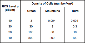

FIGURE 4.18 Number of cells with large RCS in ground clutter. Phase Zero X-band data; 2- to 12-km range; 0.5-μs pulse length.
Consider again that the clutter RCS results shown in Figure 4.18 are based on all the clutter cells within each terrain type. In a similar manner, it would certainly be possible as an alternative approach to reduce all of the Phase Zero and Phase One data in terms of clutter RCS σ rather than in terms of clutter backscattering coefficient σ°. Based on the preceding arguments that low-angle clutter is spiky and discrete, and that the RCS of a point scatterer is independent of the area of the capturing cell, it might be thought, as in the Ward and AWSE studies, that a clutter model based on reducing the measurements to σ statistics rather than σ° statistics would be the more fundamental approach. To the contrary, Section 4.5.4 will show that σ° is the fundamental quantity to which to reduce clutter measurement data for use in a spatially extensive clutter model, whether the clutter is postulated to arise from discrete or distributed sources over the surfaces involved. Before that, Section 4.5.2 provides examples of thresholded PPI clutter maps at Cochrane, further illustrating how strong isolated discrete cells appear to be embedded in spatially extensive distributed clutter at weaker levels. Then, Section 4.5.3 provides a further example of the spikey nature of low-angle clutter as measured at the prairie grassland site of Suffield and illustrates what is involved in separating one large discrete source from the background clutter when it is known what the discrete is and where it is. Section 4.5.5 provides brief conclusions concerning the practicableness of separating discrete from distributed clutter in measured data and in empirical models.
4.5.2 DISCRETE CLUTTER SOURCES AT COCHRANE
Figure 4.19 shows PPI clutter maps at Cochrane, Alberta, to 24-km maximum range based on Phase Zero X-band measurement data. The figure shows eight clutter maps at increasing thresholds of clutter strength over a dynamic range of 40 dB, from σ°F4 ≥ −48 dB to σ°F4 ≥ −8 dB. In each clutter map, cells exceeding the clutter strength threshold for that map are painted black; cells for which clutter strength is less than the threshold are left white. It is apparent in this figure that at the lowest thresholds, much of the clutter is spatially distributed over contiguous black regions much larger than a resolution cell (resolution cell size = 1° × 75 m). With increasing threshold, however, the clutter gradually becomes more spatially granular, such that at the highest thresholds shown it is apparent that the strongest cells at Cochrane are entirely spatially isolated or discrete. Similar measurements by various investigators over the years have led to a concurrence of opinion that land clutter is dominated by discrete sources, and to its often being conceptually modeled as a distributed σ° phenomenon at lower strengths augmented by discrete σ’s at higher strengths.

FIGURE 4.19(A-D) Thresholded PPI clutter plots at Cochrane, Alta. Phase Zero X-band data. Maximum range = 24 km; range resolution = 75 m. North is at zenith.
Two additional observations may be made of the data shown in Figure 4.19. First, the strong discrete clutter sources in the figure do not disappear at the long ranges first. This supports evidence and conclusions provided elsewhere in Chapter 4 that clutter strength σ° has no intrinsic dependence on range (for example, see Figure 4.11, and the plots of σ° vs range in Appendix 4.A). Secondly, it is the indication of discrete sources at the highest thresholds such as is shown in Figure 4.19 that motivates investigators to want to determine to what extent clutter modeling can be advanced by separating the effects of discretes at high levels from the more distributed clutter at lower levels. Appendix 4.D provides results obtained by going forward under this motivation and separately analyzing the effects of locally strong “discrete” cells in the measured data.
4.5.3 SEPARATION OF DISCRETE SOURCE AT SUFFIELD
This section illustrates that it is complicated to remove the effects of a single large discrete clutter source in measured clutter data, even when it is known what the discrete scatterer is and where it is situated. The investigation is conducted in repeat sector measurement data from the Suffield measurement site in southeastern Alberta. The Suffield terrain is native herbaceous rangeland. Suffield measurements were conducted in winter season with light snow cover. The landform is generally low-relief, although with some variety. From the site center the terrain gradually falls off (by 175 ft) to 7-km range, the start of the repeat sector range interval, and then gradually rises back (by 150 ft) to 13 km, the end of the repeat sector. Within the repeat sector, the low-relief terrain is largely undulating, although in places it becomes hummocky or broken. There are some small prairie sloughs or ponds in the sector (2% by area) and some low marshland areas (5% by area) surrounded by sedge and cattails. No trees, cropland, or man-made structures (except as subsequently discussed) are known to exist in the sector.
Thus, at Suffield, discrete-free clutter from winter-season grassland terrain was expected to be measured. However, the measured results appeared to be dominated by some strong discrete returns. Subsequent field surveillance determined that an Alberta Energy Corporation natural gas compressor pumping station had been built since the date of the aerial photos being utilized. The building housing the station was a large, two- to three-story, rectangular metal barn, with smaller outlying buildings and equipment, located at 8.9-km range and 127° azimuth.
The discrete clutter sources comprising the large AEC building complex were sufficient to drive the Suffield repeat sector mean clutter strengths to high levels. This is evident from the results shown in Figures 4.20 and 4.21. These figures show the same measured data reduced and plotted in different ways. Figure 4.20 shows the X-band clutter strength histogram and cumulative distribution for the Suffield repeat sector for the 15-m pulse length and at horizontal polarization. Figure 4.21 shows clutter strength vs range through the Suffield repeat sector, for the same X-band, 15-m pulse, horizontal polarization experiment, for five specific beam positions, namely, for 125.5°, 126.5°, 127.5°, and 128.5°, which are the first four contiguous beam positions in the sector, and for 134.5°, which is the last beam position in the sector (recall that the X-band beamwidth is 1°; see Table 3.A.2).

FIGURE 4.20 Clutter histogram and cumulative distribution for Suffield prairie grassland, including large discrete (metal barn). X-band, horizontal polarization, 15-m pulse. (a) Cumulative/Weibull scale and histogram/linear percent scale. (b) Histogram/logarithmic percent scale showing high-side tail.
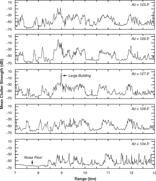
FIGURE 4.21 Mean clutter strength vs range at Suffield. Repeat sector data. X-band, 15-m pulse, horizontal polarization. Individual azimuth beam positions.
First consider the clutter histogram and cumulative distribution shown in Figure 4.20. These results were generated from partially integrated data in which each sample was obtained by coherently integrating 32 of the 1,024 pulses collected at a PRF of 2,000 Hz in each range gate with step/scan antenna positioning. In Figure 4.20(a), the histogram is plotted utilizing a linear percent ordinate; Figure 4.20(b) utilizes a logarithmic percent ordinate. The first thing to notice in the histogram is that in the clutter strength region from about −20 dB to about −50 dB, the histogram is very well behaved; the number of samples gradually diminishes with increasing strength in a very regular manner. In fact, over this region from −20 to −50 dB, the distribution of clutter strengths is very accurately represented by a Weibull distribution with a Weibull shape parameter of aw = 3.9. This well-behaved Weibull distribution of strengths measured from Suffield discrete-free grassland terrain well represents the area-extensive clutter background in these measurements.
However, the next thing to notice in the histogram, particularly as plotted in Figure 4.20(b), is that it contains a long high-side tail over the clutter strength region from −19 to +11 dB, caused by strong discrete returns of low percent occurrence. In fact, from −19 dB to +11 dB inclusive, there are 808 samples in the histogram of Figure 4.20 coming from ∼25 different spatial cells, which constitutes 0.64% of the total number of samples in the histogram. If attention is now turned to the sector display of Figure 4.21, it is evident that most of these strong values come from the vicinity of the large AEC building in the Suffield repeat sector.
The data in Figure 4.21 are now described more specifically. These data involve no spatial averaging, but show clutter strength in individual resolution cells, range gate by range gate and beam position by beam position. In each resolution cell, the clutter strength shown is the temporal mean strength resulting from averaging 32 samples, each of which is a coherent average of 32 pulses recorded at a PRF of 2,000 Hz. Generally, Figure 4.21 indicates that the clutter from this Suffield grassland terrain is of a very spiky nature, with 30-dB fluctuations common, as individual cells drop into and out of direct visibility at the low 0.3-deg depression angle involved. These data are a good example of the statistical nature of low-angle clutter, even from what is relatively homogeneous, discrete-free grassland terrain (i.e., not constant σ° or a tight Rayleigh process). Most of these clutter returns vary over the range from −20 to −50 or −60 dB. The major exception to this range of variation in the data of Figure 4.21 is the set of returns of strength ![]() −20 dB from cells in the near vicinity of the AEC building in the range interval from 8.8 to 9.0 km and at azimuths from 125.5° to 127.5°. For example, at the 127.5° azimuth position there is a strong specular flash directly from this building that raises the clutter return 30 dB or more above the envelope of the peaks in other cells not near the building. Although in the following beam position (i.e., 128.5°) no indication of the building remains, in the two preceding beam positions there is significant evidence of the building and associated discretes at levels > −20 dB spread over a number of range gates. Altogether, in these data there are 435 samples of strength ≥ −13 dB from the vicinity of the AEC building, which, if deleted, reduce the mean strength in the histogram of Figure 4.20 from −22.6 to −34.9 dB. Note that the general statistical nature of the grassland clutter at 134.5°, the final beam position in the sector, is relatively similar in range of fluctuation to that 6° earlier (i.e., at 128.5°) except over the region from 7 to 8.5 km. This region is shadowed terrain at the noise floor, where the noise level decreases with increasing range because r4 sensitivity-time-control (STC) attenuation was used in the experiment. The 5-dB discrete-finding algorithm utilized in Appendix 4.D clearly would specify a number of cells in Figure 4.21 as being “discrete,” i.e., as being 5 dB stronger than their neighbors, even though no obvious point-like discrete physical scattering sources other than the AEC building are known to exist in the Suffield repeat sector.
−20 dB from cells in the near vicinity of the AEC building in the range interval from 8.8 to 9.0 km and at azimuths from 125.5° to 127.5°. For example, at the 127.5° azimuth position there is a strong specular flash directly from this building that raises the clutter return 30 dB or more above the envelope of the peaks in other cells not near the building. Although in the following beam position (i.e., 128.5°) no indication of the building remains, in the two preceding beam positions there is significant evidence of the building and associated discretes at levels > −20 dB spread over a number of range gates. Altogether, in these data there are 435 samples of strength ≥ −13 dB from the vicinity of the AEC building, which, if deleted, reduce the mean strength in the histogram of Figure 4.20 from −22.6 to −34.9 dB. Note that the general statistical nature of the grassland clutter at 134.5°, the final beam position in the sector, is relatively similar in range of fluctuation to that 6° earlier (i.e., at 128.5°) except over the region from 7 to 8.5 km. This region is shadowed terrain at the noise floor, where the noise level decreases with increasing range because r4 sensitivity-time-control (STC) attenuation was used in the experiment. The 5-dB discrete-finding algorithm utilized in Appendix 4.D clearly would specify a number of cells in Figure 4.21 as being “discrete,” i.e., as being 5 dB stronger than their neighbors, even though no obvious point-like discrete physical scattering sources other than the AEC building are known to exist in the Suffield repeat sector.
Thus, the data of Figures 4.20 and 4.21 indicate that a more appropriate value of X-band mean clutter strength (at 15-m pulse length, horizontal polarization) to represent discrete-free Suffield grassland is −34.9 dB, not the −22.6 dB value actually measured there and driven to be so large by the presence of the AEC building. Next, similar adjustments to Suffield repeat sector mean clutter strengths are performed in other bands. These are done at low resolution (i.e., 150-m pulse length). The low resolution data are more clear-cut as to which samples come from the AEC building. Thus, in the L-band (150-m pulse, horizontal polarization) data there are four cells at σ°F4 levels of −4, −8, −16, and −17 dB providing samples (32 each) from the AEC building. When the samples from these four cells are removed from the measured histogram, the mean strength of the histogram drops from −25.0 to −39.9 dB. Similarly in the other bands (at 150-m pulse length, horizontal polarization), it is found that mean strengths adjust as follows: at X-band, from −21.7 to −33.9 dB; at S-band, from −25.3 to −43.2 dB; at L-band, from −25.0 to −39.9 dB; at UHF, from −36.8 to −40.3 dB; and at VHF, from −51.3 to −51.7 dB.
These adjusted Suffield mean clutter strengths (adjusted to be representative of grassland without the large AEC building discrete clutter source) are now compared with the grassland site of Vananda East which has similar landform (i.e., 3–5) but at which a higher depression angle occurred. This comparison is made at 150-m pulse length and horizontal polarization. At UHF, L-, and S-band, the adjusted Suffield values are remarkably close to
Vananda East values (the values are, for Suffield and Vananda East, respectively: at UHF, −40.3 dB vs −38.9 dB; at L-band, −39.9 dB vs −39.5 dB; at S-band, −43.2 dB vs −38.1 dB). Furthermore, in these three bands at both these grassland sites, mean clutter strengths are remarkably invariant with frequency at or near the −40-db level. These −40-db levels are good estimates of mean clutter strength in these bands for canonical discrete-free grassland, and therefore are what would be assigned as mean strengths to Weibull distributions for representing an area-extensive distributed clutter background.
At VHF, although Vananda East mean clutter strength holds near the −40-db level (viz., −41.7 dB), adjusted Suffield mean clutter strength drops to −51.7 dB (i.e., 10 dB weaker than Vananda East). This lower Suffield value is caused by VHF multipath loss from the hillslope local to the antenna at Suffield (see Appendix 3.B, Section 3.B.2), which does not occur for the high-bluff site at Vananda East. Note that, at VHF, the adjusted Suffield mean strength is only 0.4 dB weaker than the unadjusted value. This is because at VHF the cells containing the AEC building, although 25 to 30 dB stronger than surrounding cells, were 5 dB weaker than some cells at longer range which were strong due to multipath enhancement. This resulted in the mean clutter strength, dominated by these strong long-range cells, coincidentally being about equal to the strength of the cells containing the AEC building, so whether the AEC cells are included or not has little effect on mean clutter strength at VHF.
At X-band, the Vananda East mean clutter strength abruptly rises from the −40-db level in lower bands to −27.7 dB. This effect is described elsewhere in this book (viz., see Sections 3.4.1.5, 3.4.2, and 5.4.7.2). The adjusted Suffield X-band mean clutter strength also abruptly rises from −40 dB, but to −33.9 dB, a level 6 dB weaker than measured for grassland at Vananda East but still 11 dB stronger than measured for grassland at Big Grass Marsh.
The repeat sector values of mean clutter strength at Suffield, adjusted to be applicable to relatively discrete-free grassland by removal of cells containing the AEC building, are thus understandable and provide additional information within the context of the other discrete-free grassland sites, Vananda East (same 3–5 landform as Suffield) and Big Grass Marsh (landform = 1, level). The depression angle at Suffield, 0.3 deg, is intermediate between the depression angle at Big Grass Marsh, 0.2 deg, and that at Vananda East, 1.0 deg. As a result, at VHF and X-band, adjusted values of Suffield mean clutter strength for grassland lie intermediate between those at Big Grass Marsh and at Vananda East. At UHF, L-, and S-band, adjusted values of Suffield mean clutter strength are very nearly equivalent to those at Vananda East.
These Suffield results indicate that, in the separation of returns from a known discrete clutter source (viz., large building) in the measurement data, it is not so simple as the finding of a single large value of RCS in a single cell, but instead what is found are multiple returns from the building varying over orders of magnitude from a number of small contiguous cells, each of which partially intersects the building. This technique of separately dealing with large man-made discretes in the clutter data is usually much more demanding than at Suffield because usually many such sources exist in open terrain (e.g., farmland).
4.5.4 σ VS σ° NORMALIZATION
Section 4.5.1 raised the idea that a conceptual ground clutter model comprising (1) a σ° component for area-extensive background clutter that is distributed over all cells, augmented by (2) a σ component for discrete clutter arising from large point sources occupying a relatively small proportion of cells, is intuitively satisfying at low or high angle. However, Sections 4.5.1–4.5.3 further showed that in working with measured low-angle clutter data, which unlike clutter data at higher angles is spiky throughout, it is not readily feasible to separate a distributed σ° component known a priori to arise from physically extended surfaces from a discrete σ component known a priori to arise from physical point objects. Nevertheless, and also as illustrated in Section 4.5.1, one may choose to reduce all the measured clutter data either to clutter RCS σ per resolution cell or to normalized clutter RCS or backscattering coefficient σ° (where ![]() ; see Figure 2.4). Section 4.5.1 showed that the predilection of some previous investigators was to reduce all the measured clutter data to σ, on the basis that the stronger elements of low-angle clutter were spatially isolated or point-like (see Figure 4.19), and that the RCS σ of a point source is the fundamental quantity independent of the size of the capturing cell, as opposed to σ° which depends on the size of the capturing cell. Is it just a matter of subjective choice or preference on the part of the investigator, or do substantive reasons exist for making either σ or σ° the preferable choice to which to reduce measured low-angle clutter data?
; see Figure 2.4). Section 4.5.1 showed that the predilection of some previous investigators was to reduce all the measured clutter data to σ, on the basis that the stronger elements of low-angle clutter were spatially isolated or point-like (see Figure 4.19), and that the RCS σ of a point source is the fundamental quantity independent of the size of the capturing cell, as opposed to σ° which depends on the size of the capturing cell. Is it just a matter of subjective choice or preference on the part of the investigator, or do substantive reasons exist for making either σ or σ° the preferable choice to which to reduce measured low-angle clutter data?
For us to begin to address this question, reference is first made to the results of Section 3.5.3 in Chapter 3 showing that in measured repeat sector clutter data, the mean value of the clutter coefficient ![]() is essentially independent of cell area or spatial resolution (see Table 3.10, small differences with pulse length in all five bands). Independence of mean strength on cell area is necessary for the concept of density function to be true. It is true in the measured data, irrespective of whether descriptive adjectives like “discrete” or “distributed” are associated with the measured data, and also irrespective of whether the nature of the measured clutter is very uniform or very spiky. Thus, as described elsewhere throughout this book, the fact that
is essentially independent of cell area or spatial resolution (see Table 3.10, small differences with pulse length in all five bands). Independence of mean strength on cell area is necessary for the concept of density function to be true. It is true in the measured data, irrespective of whether descriptive adjectives like “discrete” or “distributed” are associated with the measured data, and also irrespective of whether the nature of the measured clutter is very uniform or very spiky. Thus, as described elsewhere throughout this book, the fact that ![]() is independent of cell area is fundamentally important to the structure of the modeling information presented. In contrast, if all the clutter measurement data are reduced to σ rather than σ°, the mean value of clutter RCS
is independent of cell area is fundamentally important to the structure of the modeling information presented. In contrast, if all the clutter measurement data are reduced to σ rather than σ°, the mean value of clutter RCS ![]() over a spatial region is dependent on cell area, as
over a spatial region is dependent on cell area, as ![]() . Clutter modeling information presented in terms of σ rather than σ° would require the mean values
. Clutter modeling information presented in terms of σ rather than σ° would require the mean values ![]() of clutter amplitude distributions to be shown as functions of resolution. In other words, σ is not as fundamental a quantity for specifying clutter amplitudes over extended spatial regions as is σ°.
of clutter amplitude distributions to be shown as functions of resolution. In other words, σ is not as fundamental a quantity for specifying clutter amplitudes over extended spatial regions as is σ°.
Beyond this, care must be taken not to read too much into the fact that ![]() is independent of cell area A. For example, it is easy to presume that this fact indicates that low-angle clutter is essentially not point-like but from extended surfaces—however, this is an incorrect assumption. What is indicated is that spiky clutter from discrete sources occurs distributed over surfaces; i.e., that in low-angle clutter, both adjectives apply—clutter is both “discrete” and “distributed.”
is independent of cell area A. For example, it is easy to presume that this fact indicates that low-angle clutter is essentially not point-like but from extended surfaces—however, this is an incorrect assumption. What is indicated is that spiky clutter from discrete sources occurs distributed over surfaces; i.e., that in low-angle clutter, both adjectives apply—clutter is both “discrete” and “distributed.”
It is easy to appreciate that mean clutter cross section increases linearly with cell area (i.e., ![]() ) in area-extensive clutter. But how does this observation square with the fact that in clutter arising from point sources, the more basic quantity for the cell capturing the clutter source is its RCS σ which is independent of the capturing cell size? A simple example may be illuminating in this regard. Imagine the existence of a hypothetical clutter spatial field in which each cell contains a single point discrete of σ = X. One might choose to characterize this clutter in terms of its mean clutter RCS such that
) in area-extensive clutter. But how does this observation square with the fact that in clutter arising from point sources, the more basic quantity for the cell capturing the clutter source is its RCS σ which is independent of the capturing cell size? A simple example may be illuminating in this regard. Imagine the existence of a hypothetical clutter spatial field in which each cell contains a single point discrete of σ = X. One might choose to characterize this clutter in terms of its mean clutter RCS such that ![]() . Now suppose the resolution of the radar to change so as to either increase or decrease by a factor of 10. If the resolution increases, one-tenth of the cells will capture a discrete and have σ = X; the other nine-tenths of cells will miss capturing a discrete and will have σ = 0. Thus if the resolution increases by a factor of 10,
. Now suppose the resolution of the radar to change so as to either increase or decrease by a factor of 10. If the resolution increases, one-tenth of the cells will capture a discrete and have σ = X; the other nine-tenths of cells will miss capturing a discrete and will have σ = 0. Thus if the resolution increases by a factor of 10, ![]() . If, on the other hand, the resolution decreases by a factor of 10, each cell captures 10 discretes and (under the assumption that the 10 discretes combine as a power-additive process)
. If, on the other hand, the resolution decreases by a factor of 10, each cell captures 10 discretes and (under the assumption that the 10 discretes combine as a power-additive process) ![]() . Thus even in this hypothetical discrete clutter field, mean clutter RCS
. Thus even in this hypothetical discrete clutter field, mean clutter RCS ![]() varies linearly with cell area similarly as it does in the actual measured data. That is,
varies linearly with cell area similarly as it does in the actual measured data. That is, ![]() is not an invariant irreducible quantity suitable for basing a model upon.
is not an invariant irreducible quantity suitable for basing a model upon.
Next consider the hypothetical clutter spatial field in σ° space. At the original range resolution, say 150 m, the σ° of each cell (each cell containing a single discrete of RCS = X) is ![]() . Next, allow the range resolution to increase by a factor of 10, to 15 m. Each discrete-capturing 15-m cell still provides RCS = X, and the σ° of each discrete-capturing cell rises by a factor of 10 to
. Next, allow the range resolution to increase by a factor of 10, to 15 m. Each discrete-capturing 15-m cell still provides RCS = X, and the σ° of each discrete-capturing cell rises by a factor of 10 to ![]() . But in the region around each discrete-capturing cell, there are now nine empty cells with σ° = 0. Thus the mean value of σ° over each 10-cell region is
. But in the region around each discrete-capturing cell, there are now nine empty cells with σ° = 0. Thus the mean value of σ° over each 10-cell region is ![]() which is the same value of
which is the same value of ![]() as measured with the 150-m cell. Similarly, if range resolution is allowed to decrease from its original 150-m value by a factor of 10 to 1500 m, each cell captures 10 discretes; so
as measured with the 150-m cell. Similarly, if range resolution is allowed to decrease from its original 150-m value by a factor of 10 to 1500 m, each cell captures 10 discretes; so ![]() which is also the same value of
which is also the same value of ![]() as measured with the 150-m cell.
as measured with the 150-m cell.
Thus in considering ground clutter, all possibilities of cells on the ground must be specified depending on resolution, not just cells capturing single discretes, but including possibilities of cells capturing more than one discrete and cells capturing no discretes. This is the point that is missed when intuition incorrectly suggests that σ is a more basic quantity than σ° for characterizing discrete clutter. Certainly, in a backscatter measurement of any single point object in which concern is only with the cell containing the object and not the surrounding empty cells, the appropriate characterization of the object is by its RCS σ.
This hypothetical situation of a clutter spatial field in which at intermediate resolution each cell contains a single discrete clutter source of RCS = X is handled by a σ° clutter model as follows. At all three resolutions, the mean value of clutter coefficient ![]() remains constant, invariant with cell size (as in the modeling information in this book). The different σ° distributions for the three variations in range resolution are theoretically handled through specification of differently shaped distributions for the three resolutions, but with
remains constant, invariant with cell size (as in the modeling information in this book). The different σ° distributions for the three variations in range resolution are theoretically handled through specification of differently shaped distributions for the three resolutions, but with ![]() for each distribution remaining unchanged (also as occurs in the modeling information in this book). Thus in these hypothetical situations, for the mid-size cell, the shape of the distribution is an impulse allowing no variation in σ°; for the small cell, the shape of the distribution is such as to define a two-impulse bipolar distribution with nine-tenths of the σ° values equal to zero and one-tenth equal to
for each distribution remaining unchanged (also as occurs in the modeling information in this book). Thus in these hypothetical situations, for the mid-size cell, the shape of the distribution is an impulse allowing no variation in σ°; for the small cell, the shape of the distribution is such as to define a two-impulse bipolar distribution with nine-tenths of the σ° values equal to zero and one-tenth equal to ![]() ; and for the large cell, the shape of the distribution is such as to allow the variability associated with 10 interfering scatterers within the cell. For the actual measured clutter data, as opposed to the above hypothetical construct, such extreme shapes of distributions are unnecessary; the Weibull distribution of constant mean strength
; and for the large cell, the shape of the distribution is such as to allow the variability associated with 10 interfering scatterers within the cell. For the actual measured clutter data, as opposed to the above hypothetical construct, such extreme shapes of distributions are unnecessary; the Weibull distribution of constant mean strength ![]() and varying shape parameter aw is sufficient to handle the actual variations in shape that occur with changing resolution in the actual measured data.
and varying shape parameter aw is sufficient to handle the actual variations in shape that occur with changing resolution in the actual measured data.
The above reasoning indicates that when concern is with returns from all the cells defining a surface, the correct way to empirically characterize the phenomenon is to reduce the measured data to σ°, even though each return in itself may arise from a point source. Is this reasoning supported by the observed behavior of the actual measured clutter data? Consider again that since ![]() is independent of cell area,
is independent of cell area, ![]() must increase linearly with increasing cell area. Thus in observed clutter data, if range is allowed to increase from 1 km to, say, 64 km (that is, by six factors of 2), cell area doubles with each factor of 2 increase in range leading to the expectation that clutter RCS would increase by 18 dB over this range, certainly enough to show a noticeable trend in measured data. That is, larger cells at longer ranges capture more discretes and provide larger cross sections. But in the σ° vs range results shown in this book, for example in the sector displays of Appendix 4.A or in the thresholded PPI displays of Figure 4.19, no strong trends of σ° vs range are observed, indicating that σ° is indeed the appropriate irreducible quantity upon which to base a clutter model. In all observations, σ° within visible clutter regions (although fluctuating strongly from cell to cell) neither increases nor decreases significantly with range, but remains as a fundamental quantity with range effects properly normalized out.
must increase linearly with increasing cell area. Thus in observed clutter data, if range is allowed to increase from 1 km to, say, 64 km (that is, by six factors of 2), cell area doubles with each factor of 2 increase in range leading to the expectation that clutter RCS would increase by 18 dB over this range, certainly enough to show a noticeable trend in measured data. That is, larger cells at longer ranges capture more discretes and provide larger cross sections. But in the σ° vs range results shown in this book, for example in the sector displays of Appendix 4.A or in the thresholded PPI displays of Figure 4.19, no strong trends of σ° vs range are observed, indicating that σ° is indeed the appropriate irreducible quantity upon which to base a clutter model. In all observations, σ° within visible clutter regions (although fluctuating strongly from cell to cell) neither increases nor decreases significantly with range, but remains as a fundamental quantity with range effects properly normalized out.
It is apparent from the preceding discussion that σ°, as opposed to σ, is the more fundamental quantity to which to reduce measured low-angle clutter data, despite the fact that low-angle clutter is an essentially spiky phenomenon arising from a sea of discrete clutter sources. A clutter model based on reducing all measured returns to σ is not completely reduced; such a model must include σ¯ depending on resolution as an extra complicating dimension that is not necessary in a model based on σ°. This fact leads to the clutter data in this book being reduced to σ° as the most basic characteristic of a distributed phenomenon, despite the fact that what is distributed are discrete clutter sources.
4.5.5 CONCLUSIONS
The idea behind separating discrete clutter sources in measured clutter data is that objects like water towers act as contaminants in what would otherwise be a statistically well-behaved area-extensive clutter background from the land surface itself, and that a better clutter model results if RCS values of strong discretes are added in a separate σ process to the basic distributed σ° component representing the background clutter. This idea has some validity at higher angles of illumination typical of airborne radar platforms. At the low angles of illumination of ground-based radars, the focus of the idea tends to dissipate for several reasons. First, low-angle clutter is spiky throughout; removal of the largest spikes still leaves a spiky background. Second, it is not possible to deterministically separate clutter arising from point objects from clutter arising from extended surfaces in the measured data. Many spikes occur only because of vicissitudes of visibility and shadowing compounded by extreme propagation variations at very low angles of illumination. Little correlation exists between locally strong clutter returns and known point objects on the ground. Third, even though low-angle clutter appears to arise from a sea of discretes, the proper way to reduce the data is to the normalized clutter coefficient σ°, as opposed to radar cross section σ, irrespective of whether one is examining so-called “distributed” or “discrete” components.
Given these qualifications, if we continue to wish to examine the usefulness of separately analyzing and modeling strong clutter as an overlay to the general clutter background, it is necessary to fall back to a position in which locally strong cells are specified a posteriori in the measured clutter data as opposed to their a priori specification as the returns from known point objects.
In so doing, the initial premise has changed. Rather than removing and separately modeling the returns from known point discretes such as water towers, the question now being posed is if it is useful to model the total clutter distribution from a given spatial region as two components, one consisting of the locally strong clutter cells resulting from passing a spatial filter over the data and the other consisting of the residual clutter cells which failed to pass the filter. That is, is it useful to set a threshold so as to separate locally strong σ° from weaker surrounding σ°. The potential benefit of such a procedure hinges on the possibility of there being a difference in kind, not just degree, in the two distributions (even though each consists of spiky returns) such that each might be of a relatively simple shape, whereas their combination is of a more complex shape. Note that both components are broad distributions consisting of spiky returns of strengths differing by orders of magnitude, with the major differences being that the so-called “discrete” component consists of locally strong spiky returns and the so-called “background” component consists of the weaker neighboring spiky returns. Further, note that there is no benefit and indeed needless added complexity in moving to σ space to characterize the locally strong or so-called “discrete” component.
The modeling of clutter based on the two-distribution approach allows the possibility of assigning two random variates to each clutter cell with the resulting total σ° being the phasor addition of the two components. This approach models “discrete” clutter returns statistically rather than attempting to deterministically specify returns from known point targets on the landscape. Appendix 4.D shows results obtained from separating clutter into two σ° components in this manner. The main approach of this book, however, is to characterize the total clutter from a given spatial region as a single Weibull distribution, where the broad extent of the Weibull distribution usually satisfactorily represents the measured distribution, capturing the occasional strong returns from discrete sources at appropriate probabilities of occurrence. The clutter modeling information provided in Chapter 5 and elsewhere (except in Appendix 4.D) in this book is based on the single-distribution approach involving the assignment of a single random variate to represent clutter strength in each resolution cell.
4.6 TEMPORAL STATISTICS, SPECTRA, AND CORRELATION
For many years, in radars of low spatial resolution, the in-phase and quadrature components of the spatially varying ground clutter signal were considered to be distributed as Gaussian probability density functions, resulting in the signal amplitude being Rayleigh distributed (see, for example [12], Section 10.2). In modern radar systems, operating at low grazing angles and with resolution capabilities high enough to resolve the surface structure, the statistics of the clutter have been observed to strongly deviate from Gaussianity [13–19]. The clutter is spikier than if it were Gaussian, and the spikes are processed by the radar detector as targets, with increased false-alarm rate. Until now, Chapter 4 and the preceding chapters of this book have been primarily concerned with the characterizations and prediction of the highly non-Gaussian clutter amplitude statistics resulting from cell-to-cell spatial variations in ground clutter signals.
Windblown ground clutter Doppler spectra also in early years were, like the amplitude distributions, erroneously thought to be of Gaussian shape [20–22]. The correct understanding of ground clutter and the accurate modeling of its non-Gaussian behavior, both in the spatial amplitude distribution and in the Doppler spectrum, are problems of fundamental interest to the radar community for successful radar design and performance prediction. The subject now widens to include temporal variations in the received clutter signals returned from particular spatial cells. Important attributes of temporal statistics are (1) temporal amplitude statistics, (2) spectral characteristics, and (3) correlation times. Correlation distance in the ground clutter spatial process is also discussed. Improved knowledge of these various additional attributes of ground clutter, in addition to its spatial amplitude statistics, is required in the demanding specialized design of modern signal processors required to detect, track, and otherwise operate against ever-smaller radar targets in ground clutter backgrounds. For example, the spectral characteristics of clutter determine the design of moving target indicator (MTI) or space-time adaptive processors (STAP) [23, 24], and the amplitude statistics of clutter affect the design of constant-false-alarm rate (CFAR) processors (see e.g., [12, p. 306; 25]).
Results concerning these additional important attributes of low-angle ground clutter are provided in Section 4.6 at a first or introductory level of analysis. More in-depth analyses of these attributes based on the Phase One clutter data are available elsewhere [26–31]. They show that the temporal and spatial domains of ground clutter are interrelated. However, in the specification of the spatial clutter amplitude statistics which is a principal focus of this book, each individual spatial clutter amplitude so specified may be regarded as the mean level of a temporal process in a given spatial cell. Subsequently, Chapter 6 takes up the subject of the modeling of windblown ground clutter spectral shape as a second principal focus of this book.
4.6.1 TEMPORAL STATISTICS
Figure 4.22 presents information describing the relative frequency of occurrence of temporal amplitude statistics between cells with Rayleigh (i.e., windblown foliage) and Ricean (i.e., fixed discretes embedded in foliage) statistics. Ricean statistics describe ground clutter temporal variations from a fixed spatial cell quite accurately as the return of a dominant steady reflector or fixed discrete in a varying background [22, 32]. Rayleigh statistics are a limiting case of Ricean statistics with steady signal equal to zero. The quantity m2 in the Ricean distribution as introduced by Goldstein [22] is the ratio of steady to random average power, or, in other words, the dominant-to-Rayleigh reflector ratio. The ratio of standard deviation-to-mean (sd/mean) in the Ricean process is related to ![]() .
.

The data in Figure 4.22 indicate that, over a population of 988 relatively strong clutter cells selected from three rural sites, more than 40% of the cells are Rayleigh (i.e., have ratios of standard deviation-to-mean = 0 dB), and the remainder are generally Ricean (i.e., have ratios of standard deviation-to-mean < 0 dB), with increasingly strong Ricean cells occurring less frequently. For example, Figure 4.22 shows that 1% of cells are strongly enough dominated by fixed discretes to have a dominant-to-Rayleigh reflector ratio as high as 50. The reason that 40% of the clutter cells in the figure contain only windblown foliage with dominant-to-Rayleigh reflector ratio equal to zero is that there are some trees on these farmland landscapes. Where trees occur, even at relatively low incidence of occurrence, they tend to dominate as strong clutter sources (see Chapter 2, Section 2.4.2.5).
4.6.2 SPECTRAL CHARACTERISTICS
For Rayleigh cells containing windblown trees, the wind-induced motion causes Doppler-shifted energy in the power spectra of the received temporal signals. Figure 4.23 shows two examples of windblown ground clutter spectral results, each computed from a Phase One X-band long-time-dwell experiment measured from the same forested cell at 2.6-km range on two April days about one week apart. This cell contains mixed deciduous and evergreen trees to an approximate height of 60 or 70 ft. On the first day, 17 April, the winds were quite strong; at the time of this X-band experiment, wind speed was recorded at 10 knots, gusting to 20. In contrast, the second day, 25 April, was a very still day and the winds were recorded as calm at the time of the experiment.

The spectra of Figure 4.23 are computed directly as fast Fourier transforms (FFTs) of the temporal pulse-by-pulse return, including the dc component, calibrated in radar cross section (RCS) units of meters squared. The spectral content is displayed in decibels with respect to 1 m2 (i.e., in dBsm). The method used to generate these spectra is that of modified periodograms [33], where the temporal record of 30,720 pulses is divided into continuous groups of 1,024 samples, a 1,024-point complex FFT is generated for each group, and the amplitudes of the resultant set of FFTs are arithmetically averaged together in each Doppler cell to provide the spectrum illustrated. Thus in Figure 4.23 each spectrum shown is the result of averaging 30 individual spectra from an overall RCS record of 1.024-min duration and 2-ms pulse repetition interval (PRI). In the generation of each spectrum, a 4-sample Blackman-Harris window or weighting function is utilized, with highest sidelobe level at −74 dB and with 6-dB per octave fall-off [34].
The results of Figure 4.23 illustrate the differences in spectral content of the X-band reflections from this cell between when the tree branches are relatively motionless and when they are undergoing relatively strong, wind-induced, random motion. It is graphically apparent in these results how much of the dc or zero-Doppler return on the calm day is converted to ac return distributed over Doppler velocities up to 2 m/s on the windy day. The windy day spectrum shown in the figure is one of the wider spectra found in the Phase One long-time-dwell clutter database. In this windy day data, the rate of decay of spectral energy with increasing Doppler velocity in the tail of the spectrum is approximately exponential as indicated by the straight line drawn through the left side of the spectrum. The Phase One system noise levels are evident in both the calm and windy day results of Figure 4.23 at a level of about −64 dBsm. Andrianov, Armand, and Kibardina [35] provide an earlier observation of piece-part exponential spectral decay in windblown radar ground clutter Doppler spectra (see Section 6.6.1.3).
The results of Figure 4.23 are representative of much of the Lincoln Laboratory clutter spectral data, in that rates of decay of spectral power with increasing Doppler velocity in radar returns from windblown trees in these data are often observed to be reasonably well approximated as exponential. One Phase One study [26] involved fitting exponential approximations to 23 different Phase One L-band experiments obtained from nominally once-a-week measurements over a period of nine months, to provide information on how clutter spectra vary with wind, weather, and season. Chapter 6 takes up the matter of windblown clutter spectral modeling much more extensively and completely.
4.6.3 CORRELATIVE PROPERTIES
The question now is, how long does it take for radar returns from windblown trees to decorrelate? This question is complementary to that of spectral extent in such returns. The normalized autocorrelation function [36] was computed for all five Phase One frequencies for the returns from the same 2.6-km forested cell as measured on the windy day of 17 April [26] for which spectral results are shown in Figure 4.23. These autocorrelation results are shown in Figure 4.24 over a time lag from 0 to 0.5 sec. The time of day (hr:min) at which data collection commenced for each of these five long-time-dwell experiments was as follows: X-band, 10:24; S-band, 11:30; L-band, 14:12; VHF, 15:50; UHF, 15:27. Each of these five long-time-dwell experiments consisted of 30,720 pulses at PRIs of 2, 10, 10, 6, and 2 ms for VHF, UHF, L-, S-, and X-bands, respectively. For all five experiments, the polarization was horizontal and the range resolution was 150 m. At each of the five Phase One frequencies, the autocorrelation of the return from a stationary water tower reference target remains essentially at unity over the 0.5-s time lag shown in Figure 4.24. Correlation times τ1/e and τ1/2 are defined as the times required for the normalized autocorrelation function to decrease to 1/e (= 0.368) or 1/2 (= 0.5), respectively. Table 4.10 gives these measures of time required for decorrelation of the radar returns from windblown trees, as determined from the data of Figure 4.24.
TABLE 4.10
Correlation Times for Radar Returns from Windblown Trees on a Windy Day
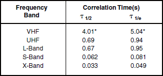
*Note: = extrapolated estimate

FIGURE 4.24 Autocorrelation functions of radar returns from windblown trees on a windy day at five radar frequencies.
If the scattering centers and their motion were the same at all five frequencies, simple Doppler considerations would lead to the expectation that correlation times should decrease inversely with radar carrier frequency, all else being equal. There is an approximate trend indicative of this effect in the data of Figure 4.24 and Table 4.10. These results do not scale exactly linearly with frequency, however, because (1) the experiments were conducted at different times and thus under different specific wind conditions on 17 April, (2) the cell sizes and hence scattering center ensembles were different (e.g., due to azimuth beamwidth varying with frequency band), and (3) the scattering centers and their velocities are expected to vary with the radar transmission wavelength (i.e., twigs at X-band, branches at L-band, limbs at VHF).
The correlative properties of radar returns from windblown trees shown in Figure 4.24 and Table 4.10 apply for the particularly windy day of 17 April. Correlation times from windblown trees increase with decreasing wind speed. Figure 4.25 shows the normalized autocorrelation function for the L-band returns from the same 2.6-km forested cell, measured on three different days under three quite different wind conditions. The autocorrelation function is shown in Figure 4.25 only over the correlation interval from 1.0 to 0.9 to emphasize the region where the data just begins to decorrelate. In Figure 4.25, the windy day was 17 April (wind speed = 15 to 25 kn), the breezy day was 10 April (wind speed ≈11 kn), and the light air day was 5 June (wind speed ≤ 8 kn). Each of these long-time-dwell experiments consisted of 30,720 pulses at pulse repetition intervals of 10, 2, and 10 ms for the windy, breezy, and light air days, respectively. In these results, the correlation times τ1/e on the windy, breezy, and light air days were 0.95, 2.11, and 5.56 s, respectively. These results show how temporal correlation in L-band radar returns from windblown trees increases with decreasing wind speed.

FIGURE 4.25 Autocorrelation functions of L-band radar returns from windblown trees for three different wind conditions.
Spatial Correlation. In contrast to temporal correlation, which addresses the question of duration in time that must pass for a clutter signal from a fixed cell to decorrelate, spatial correlation addresses the question of extent in distance (i.e., number of cell dimensions) that must be traversed in order that the clutter signal from the current cell decorrelates with respect to the signal from the original cell. Because of the general spatial heterogeneity of terrain and the spiky spatial nature of the land clutter phenomenon as observed at low angles, a number of studies over the course of the Phase Zero/Phase One activities have found that low-angle land clutter often spatially decorrelates in about one spatial cell. That is, the physical content (i.e., scattering ensemble) within each cell when observed at low angles is usually different enough (different set of discrete sources) from cell to cell that the signal from any one cell largely decorrelates from its spatial neighbors. Occasionally, increased correlation is observed from cell to cell, for example, at higher angles over uniform forest.
As an example of cell-to-cell spatial decorrelation, results are summarized here from a statistical study [30] of Phase One X-band open farmland clutter data collected at the Wolseley, Saskatchewan site.25 Other results from this study are discussed in Appendix 5.A. The data were acquired in slow (2°/s) scan mode through one ∼90° azimuth sector in which 703 azimuth samples were collected per range cell. Within the azimuth sector, data were acquired in four contiguous 4.74-km range intervals; each range interval contained 316 range cells of 15 meter sampling interval (i.e., 10 MHz sampling rate). Figures 4.26 and 4.27 show azimuth and range spatial correlation coefficients obtained in processing the fourth range interval in these data. The results were obtained by processing the entire 703 × 416 sample array of data obtained at HH-polarization in the fourth range interval (15.2 to 20.0 km from the radar).

FIGURE 4.26 Azimuthal correlation coefficient, fourth-range interval, HH polarization. (Results provided by F. Gini and M. Greco, Univ. of Pisa. After [30]; by permission, © 1999 IEEE.)
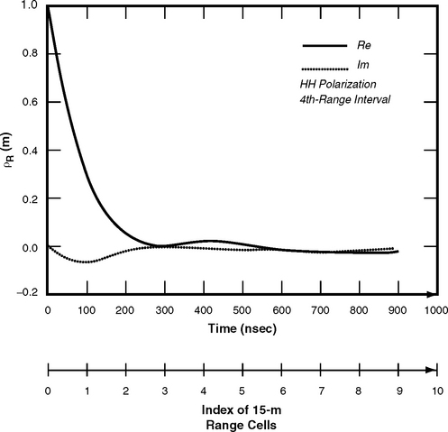
FIGURE 4.27 Range correlation coefficient, fourth range interval, HH polarization. (Results provided by F. Gini and M. Greco, Univ. of Pisa. After [30]; by permission, © 1999 IEEE.)
The azimuthal autocorrelation sequence was estimated from the data without making any assumption, other than stationarity, about the structure of the clutter process. The sample estimator processed M = 316 records {zk}Mk= 1, one for each range cell, of N = 703 complex azimuth samples according to the following algorithm [37, Ch. 9]:
where zI(n) and zQ(n) are the in-phase and quadrature components, z(n) = zI(n) + jzQ(n) is the complex envelope of the observed signal, and * represents complex conjugate. In Figure 4.26 the correlation coefficient ![]() is shown for the fourth range interval. It is observed that the signal decorrelates to 0.29 in one 1°-beamwidth, and to ∼0 in four beamwidths. As expected, the imaginary part of ρz(m), i.e., the cross-correlation coefficient
is shown for the fourth range interval. It is observed that the signal decorrelates to 0.29 in one 1°-beamwidth, and to ∼0 in four beamwidths. As expected, the imaginary part of ρz(m), i.e., the cross-correlation coefficient ![]() , is approximately zero.
, is approximately zero.
To obtain the range correlation coefficient, the correlation for each azimuth cell was calculated, and then the 703 estimates were averaged. The correlation coefficient ρR(m) is plotted in Figure 4.27. Comparing this figure with Figure 4.26, the two decorrelation times are observed to be quite different. Along the azimuth direction the coefficient reduces to 0.1 in a few seconds, whereas along the range direction, the same amount of reduction occurs in a few hundreds of nanoseconds. These apparent large differences are merely the result of the different time-sampling frequencies utilized in range (10 MHz) and in azimuth (15.625 Hz). The assumption usually made in adaptive radar detection (see, e.g., [38], Ch. 3) of independence of the data from different range cells is very reasonable in these Wolseley data.
Thus, the important thing to observe in considering Figures 4.26 and 4.27 is that, owing to the heterogeneity of the spatial scattering ensemble in open farmland terrain (strong discrete sources dispersed over a weakly scattering medium), the returned signal from the scanning antenna largely decorrelates from one spatial cell to the next, whether the variation is in the range direction or in the azimuth direction. Consider again the azimuth variation results of Figure 4.26. The azimuth extent of the spatial resolution cell is determined by the beamwidth of ∼1°. The scan rate is 2°/s, so the expectation is that the returned signal would decorrelate in ∼1 beamwidth or ∼0.5 s. Figure 4.26 shows the azimuthal correlation coefficient to drop to 0.29 in 0.5 s (one beamwidth), but to take ∼2 s (∼4 beamwidths) to decorrelate to zero. This largely meets the expectation of decorrelation in one azimuthal interval, given that the azimuthal cell specified is the 3-dB beamwidth, with resultant beam overlap between 1° cells. The azimuth sampling rate used in data acquisition was 15.625 samples (pulses) per second. That is, in azimuth, the sampling time (0.064 s, is much less than the cell size (∼0.5 s).
Now consider again the range variation results shown in Figure 4.27. The range extent of the spatial resolution cell is determined by the 3-dB pulse length which is specified to be 100 ns. This is matched to the range sampling rate of 10 MHz (i.e., in range, the sampling interval equals the cell size). Therefore, the expectation is that, in range, the returned signal would largely decorrelate, sample-to-sample, in ∼100 ns. Figure 4.27 shows the range correlation coefficient to drop to 0.3 in 100 ns (one pulse length), but it takes 300 ns (3 pulse lengths) to decorrelate to zero. Thus the range results of Figure 4.27 very closely match the azimuthal results of Figure 4.26 in terms of equivalent cell-to-cell decorrelation in azimuth and range.
Note that although the azimuthal decorrelation in Figure 4.26 is caused by the antenna pattern, the decorrelation data cannot be simply predicted from the pattern. Perhaps it would be useful to state a simple example as follows: if the pattern were hypothetically purely rectangular (i.e., a simple step function of width ϕ), and if the clutter were simply one large point scatterer, then the azimuthal correlation coefficient would be triangular of base width 2ϕ (i.e., would fall to 0.5 in one cell and to zero in two cells). By contrast, the measured data in Figure 4.26 falls to 0.29 in one cell and to zero in four cells.