
6.6 HISTORICAL REVIEW
6.6.1 Three Analytic Spectral Shapes
In comparing different analytic forms for the shape of the ac component of the windblown clutter Doppler velocity spectrum Pac(v) [see Eq. (6.1)], it is necessary to base the comparison on equivalent total ac spectral power, and it is convenient to maintain total ac spectral power at unity. Such normalization is seldom implemented in representations of clutter spectra. Figure 6.44 shows examples of the three forms for Pac(v) to be discussed subsequently, namely Gaussian, power law, and exponential, in each of which

As a result, the power density levels at any value v for these three spectral shapes as shown in Figure 6.44 are directly comparable on an equivalent total ac power basis.
The ac spectral shape function Pac(v) may be decomposed as
where η is a shape parameter, Kη is a normalization constant set so that
and kη (v) is the unnormalized shape function with kη (0) = 1. Often, historically, Kη is omitted and only kη (v) is shown in plots such as Figure 6.44 with the zero-Doppler peak at 0 dB. In such cases, at best the shape parameter η of each individual spectral representation is all that remains for adjustment to equivalent total ac spectral power, where in fact it is the shape parameter that should be used to match to experimental data, or at worst (often the case) no attempt is made to compare spectra on an equivalent total ac spectral power basis at all. In short, in comparing different analytic spectral representations, it is not rigorously proper to simply set their zero-Doppler peaks each at unity (i.e., 0 dB).
In the examples shown in Figure 6.44, spectral extent of the exponential representation lies between that of the Gaussian (narrow) and that of the power law (wide). The following subsections consider the origins of these three analytic expressions that have been used in the past to represent the shape of the Doppler frequency or velocity spectrum of windblown ground clutter, and in particular the rate of decay with increasing Doppler in the tail of the spectrum. It is evident in Figure 6.44 that the historical Gaussian and power-law representations match the Lincoln Laboratory-based exponential representation reasonably well (i.e., at least to within an order of magnitude) over the upper levels of clutter spectral power that lie within the dynamic ranges (solid lines) of these historical measurements; but that extrapolations of the historical representations (dotted lines) to much lower levels of spectral power differ by many orders of magnitude from the Lincoln Laboratory measurements at these low levels.
6.6.1.1 GAUSSIAN SPECTRAL SHAPE
Radar ground clutter power spectra were originally thought to be of approximately Gaussian shape [6–9]. The Gaussian spectral shape may be represented analytically as
where g is the Gaussian shape parameter, ![]() is the normalization constant, k(v) = exp(–gv2), and
is the normalization constant, k(v) = exp(–gv2), and
To convert to Pac(f) in Eq. (6.17) where f is Doppler frequency, i.e., Pac(f) df = Pac(v)dv, replace v by f and g by (λ/2)2g. The standard deviation of the Gaussian spectrum of Eq. (6.17) is given by ![]() in units of m/s. In a much-referenced [1, 27, 50] early paper, Barlow [7] presents measured L-band ground clutter power spectra approximated by the Gaussian shape to a level 20 dB below the peak zero-Doppler level and to a maximum Doppler velocity of 0.67 m/s. Figure 6.45 shows Barlow’s ground clutter spectra k(v) as plotted originally, except here vs Doppler velocity v rather than Doppler frequency f. Recall that k(v) is the unnormalized ac shape function such that k(0) = 1, so the spectra plotted in Figure 6.45 are not shown on an equivalent total ac power basis.
in units of m/s. In a much-referenced [1, 27, 50] early paper, Barlow [7] presents measured L-band ground clutter power spectra approximated by the Gaussian shape to a level 20 dB below the peak zero-Doppler level and to a maximum Doppler velocity of 0.67 m/s. Figure 6.45 shows Barlow’s ground clutter spectra k(v) as plotted originally, except here vs Doppler velocity v rather than Doppler frequency f. Recall that k(v) is the unnormalized ac shape function such that k(0) = 1, so the spectra plotted in Figure 6.45 are not shown on an equivalent total ac power basis.
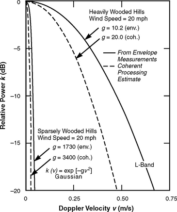
FIGURE 6.45 Measurements of radar ground clutter power spectra by Barlow. (After [7]; by permission, © 1949 IEEE.)
Barlow’s spectral results were obtained from radar envelope measurements as opposed to coherent processing. For a Gaussian-shaped spectrum, the width of the envelope spectrum is approximately 1.4 times the width of the coherent spectrum [51,52]. That is, in Eq. (6.17), gcoherent ≈ (1.4)2 genvelope. On this basis, estimates of the shapes of the coherent spectra corresponding to Barlow’s envelope spectra are also shown in Figure 6.45. The resulting g = 20.04 coherent-spectrum k(v) curve shown in Figure 6.45 for heavily wooded hills under 20 mph winds corresponds to the Gaussian g = 20 Pac(v) curve shown in Figure 6.44.
Early observations at the MIT Radiation Laboratory [8, 9] were that the shapes of power spectra from precipitation, chaff, and sea echo were “roughly Gaussian” and that the shape of the spectrum from land clutter was “roughly similar” but with differences from Gaussian shape “somewhat more pronounced.” The explanation for clutter spectra of approximately Gaussian shape is loosely based on the idea that windblown vegetation consists fundamentally of a random array of elemental moving scatterers, each with a constant translational drift velocity. If the distribution of radial velocities of such a group of scatterers were approximately Gaussian, they would generate an approximately Gaussian-shaped power spectrum. However, consider if the motion of the scatterers also were to include an oscillatory component to represent branches and leaves blowing back and forth in the wind. It is well known [53] that simple harmonic angle modulation (frequency or phase) generates an infinite series of sidebands so that an array of oscillating scatterers would be expected to generate a wider spectrum than an array of scatterers each with only a constant drift velocity.
Indeed, in 1967 Wong, Reed, and Kaprielian [29] provided an analysis of the scattered signal and power spectrum from an array of scatterers, each with random rotational (oscillatory) motion as well as a constant random drift velocity. Under assumptions of Gaussianly distributed drift and rotational velocities, Wong et al. [29] showed that the power spectrum of the scattered signal is the sum of six components. Li [19] subsequently provided further interpretation of these six components, as follows. If scatterer rotation is absent, the Wong et al. expression for the clutter spectrum degenerates to Barlow’s simple Gaussian expression, i.e., Eq. (6.17). However, with scatterer rotation present, five additional Gaussian components arise, all of which decay more slowly and all but one of which are offset from zero-Doppler (by ± 2 and ± 4 times the rotational velocity). As a result, these five additional Gaussian terms that come into play with scatterer rotation act to “spread” the spectrum beyond that of the simple Gaussian of Eq. (6.17). Narayanan et al. [42] returned to Wong’s formulation of offset Gaussians in modeling some later-acquired X-band windblown clutter spectral measurements.
In 1965, two years before the publication of the Wong et al. paper [29], Bass, Bliokh, and Fuks [54] also provided a theoretical study of scattering from oscillating reradiators to model scattering from windblown vegetation. In the Bass et al. paper, the reradiators were modeled to be decaying oscillators randomly positioned on a planar surface. In their analysis, Bass et al. showed that the power spectrum of the scattered radiation from the oscillating reradiators consists of a doubly infinite sum of offset Gaussian functions, but when the reradiators do not oscillate, the power spectrum simplifies to a sum of simple non-offset Gaussians. It is evident that these results have some degree of similarity with those of Wong et al. [29] in that both represent the power spectrum from a group of oscillating random scatterers as sums of Gaussians, the peaks of which are offset from zero-Doppler and for which the offsets collapse in the absence of oscillation.
Some years following both the Wong et al. [29] and the Bass et al. papers [54], Rosenbaum and Bowles [55] derived theoretical expressions for windblown clutter spectra based on a physical model in which the backscattering was associated with random permittivity fluctuations superimposed on a lossy background slab. Again with overtones of similarity to both the Wong et al. and the Bass et al. analyses, Rosenbaum and Bowles modeled scatterer motion two ways, first, as a Gaussian process, and second, assuming scatterer motion to be quasi-harmonic, so that the scatterers behave as decaying simple-harmonic oscillators. It has been observed that the Rosenbaum and Bowles spectral results “are … too complex for radar engineers to use in design practice” [19].
Status (Gaussian Spectral Shape). As will be shown, essentially all measurements of ground clutter spectra from 1967 on, of increased sensitivity compared with those of Barlow and the other early investigators, without exception show spectral shapes wider in their tails than Barlow’s simple Gaussian. Also, as indicated in the preceding discussion, it had become theoretically well understood, also from 1965–67 on, that scatterer rotational and/or oscillatory motion generates spectra wider than Gaussian. Nevertheless, Barlow’s simple Gaussian representation continues to be how clutter spectra are usually represented in radar system engineering, at least as a method of first-approach in representing the effects of intrinsic clutter motion. Thus many of the standard radar system engineering and phenomenology textbooks continue to reference Barlow’s early results [1, 27, 50].
Also, Nathanson [28] characterizes ground clutter spectral width in a scatter plot of data from many different sources in which the standard deviation in the best fit of each data source to a Gaussian shape is plotted vs wind velocity. Although it is stated in Nathanson that these results are not intended as a recommendation for the use of Gaussian spectral shape in any system design in which the detailed shape of the spectrum is of consequence, nevertheless Nathanson’s results continue to be referenced as justification for the “common assumption …” [4] that the internal-motion clutter spectral shape is Gaussian (see also [56] for a similar remark). This continuing representation is understandably based on reasons of simplicity, i.e., “the clutter spectrum is often modeled as Gaussian for convenience, but is usually more complex” [57], and analytic tractability, e.g., the Gaussian function is its own Fourier transform [51].
6.6.1.2 POWER-LAW SPECTRAL SHAPE
MTI system performance predicted by the assumption of a Gaussian-shaped clutter spectrum was not achieved in practice. In a much referenced later report, Fishbein, Graveline, and Rittenbach [10] introduced the power-law clutter spectral shape. The power-law spectral shape may be generally represented analytically as

Equation (6.18) has two power-law shape parameters—n, the power-law exponent, and vc, the break-point Doppler velocity where the shape function is 3 dB below its peak zero-Doppler level. The normalization constant K is equal to nsin(π/n)/(2πvc); k(v) = 1/[1 + (|v|vc)n]; and
To convert to Pac(f) in Eq. (6.18), i.e., Pac(f)df = Pac(v) dv, replace v by f and vc by fc = (2/λ)vc. For velocities > v > vc, Eq. (6.18) simplifies to ![]() , which plots as a straight line in a plot of 10 log Pac vs log v. In such a plot, n defines the slope of the straight-line v−n power-law spectral tail (slope = dB/decade = 10 n). Because of its two shape parameters, the power-law shape function of Eq. (6.18) has an additional degree of freedom for fitting experimental data compared with the single-parameter Gaussian and exponential shape functions of Eqs. (6.17) and (6.2), respectively. For any power of n, the power-law shape function may be made as narrow as desired by making vc small enough. Still, whatever the values of n and vc, ultimately at low enough power levels (i.e., as 10logP → −∞) the power-law shape always becomes wider than Gaussian or exponential.
, which plots as a straight line in a plot of 10 log Pac vs log v. In such a plot, n defines the slope of the straight-line v−n power-law spectral tail (slope = dB/decade = 10 n). Because of its two shape parameters, the power-law shape function of Eq. (6.18) has an additional degree of freedom for fitting experimental data compared with the single-parameter Gaussian and exponential shape functions of Eqs. (6.17) and (6.2), respectively. For any power of n, the power-law shape function may be made as narrow as desired by making vc small enough. Still, whatever the values of n and vc, ultimately at low enough power levels (i.e., as 10logP → −∞) the power-law shape always becomes wider than Gaussian or exponential.
Fishbein et al. [10] indicate that measured clutter rejection ratios up to 40 dB are matched under the assumption of a theoretical power-law spectral shape with n = 3. They also made one actual X-band clutter spectral measurement in 12 knot winds verifying that an n = 3 spectral tail did exist down to a level 35 dB below the zero-Doppler level and out to a maximum Doppler velocity of 1.6 m/s. The graph of these results, shown in Figure 6.46, appears to very convincingly show the clutter spectrum to be an n = 3 power law, as opposed to Gaussian, and it is widely referenced [27, 28].
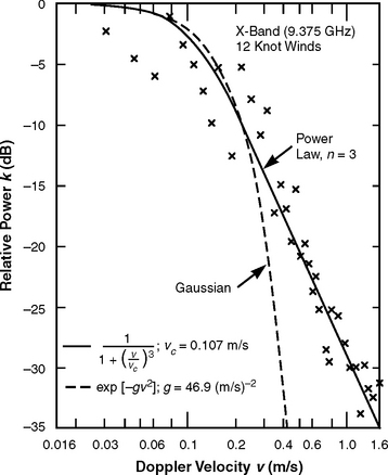
FIGURE 6.46 A measured radar ground clutter power spectrum by Fishbein, Graveline, and Rittenbach of the U. S. Army Electronics Command. After [10], 1967.
The Gaussian and power-law curves in Figure 6.46 are k(v) curves as originally presented by Fishbein et al. [10] with their zero-Doppler peaks at 0 dB. Such k(v) curves are generally not of equivalent total ac power. However, the particular Gaussian curve shown in Figure 6.46 is the one resulting when its shape parameter g is adjusted to the necessary value, viz., g = 46.9, to provide equivalent power (not unity) to that contained by the power-law curve of Figure 6.46. That is, the Gaussian curve in this figure did not arise from direct fitting to measured data. In contrast, Barlow’s Gaussian curves of Figure 6.45 did arise from direct fitting to measured data. It is more fair to compare the Fishbein et al. n = 3 power-law curve of Figure 6.46 with Barlow’s g = 10 and 20 Gaussian curves of Figure 6.45, all as Pac curves normalized to unit total ac spectral power for whatever values of shape parameter were required to fit to measured data. The g = 20 Gaussian curve and n = 3, vc = 0.107 power-law curve shown in Figure 6.44 are Barlow and Fishbein et al. curves, respectively, plotted as Pac functions, each properly normalized to equivalent unit total ac spectral power. It is evident that Barlow’s g = 20 Gaussian curve would be considerably wider than (i.e., would lie to the right of) the g = 46.9 Gaussian plotted in Figure 6.46, with the result that the data in Figure 6.46 become somewhat less convincingly power law.
The Fishbein et al. [10] results were important in establishing the existence of low-level tails wider than Gaussian in ground clutter spectra. Other ground clutter spectral measurements followed in which power-law spectral shapes were observed. For example, shortly after publication of the Fishbein et al. report, Warden and Wyndham [11] briefly mentioned two S-band measurements of clutter spectra, shown in Figure 6.47. The first was a clutter spectrum for a wooded hillside in 14- to 16-knot winds. The shape of this spectrum, to −29 dB at a maximum Doppler velocity of 0.82 m/s, is wider than Gaussian but narrower than an n = 3 power law. The second was a clutter spectrum for a bare hill in 10- to 12-knot winds. This spectrum is slightly narrower than the first, although still wider than Gaussian in the tail. The authors concluded that an n = 3 power law best fitted their data overall.

FIGURE 6.47 Two measurements of radar ground clutter power spectra by Warden and Wyndham of the Royal Radar Establishment (U. K.). After [11], 1969.
Several years later, Currie, Dyer, and Hayes [12] provided measurements of noncoherent clutter spectra from deciduous trees under light air and breezy conditions over a spectral dynamic range of 20 dB at frequencies of 9.5, 16, 35, and 95 GHz. Over this limited spectral dynamic range, they also found their results to be well fitted with power laws of n = 3 in the lower bands and n = 4 at 95 GHz. At both 9.5 and 16.5 GHz, maximum spectral extents under breezy 6- to 15-mph winds at the −20-dB level were ∼0.8 m/s, which is a close match both to the Fishbein et al. results and to the Phase One and LCE measurements and exponential model (see Figure 6.1) of Chapter 6 over similar spectral dynamic ranges and under similar breezy conditions—especially if the Currie et al. spectral widths are reduced by a factor of ∼1.4 to account for the fact that their measurements were noncoherent. At 35 and 95 GHz, maximum spectral extents under breezy conditions at the −20-dB level were ∼0.5 m/s, that is, ∼40% narrower than at the lower X- and Ku-band frequencies. These narrower upper-band spectra appear to indicate that the frequency invariance, VHF to X-band, of Doppler-velocity ac spectral shape of the current exponential model may not extend to frequencies as high as 35 GHz (Ka-band) and 95 GHz (W-band). The Currie et al. [12] results are also discussed in Long [27] and in Currie and Brown [58]; in the latter discussion, Currie remarks that “curve-fitting is an inexact science” and raises the possibility that other spectral shapes might also have been used to equally well fit these data.
A set of papers in the Russian literature [13–16] from the same time period included power law among various analytic representations used in fitting experimental data in different Doppler regimes. Results taken from these Russian papers are shown in Figures 6.48, 6.49, and 6.50. In these Russian studies, spectral power was observed to decay at first according to Gaussian [13] or exponential [16] laws to spectral power levels down 10 to 20 dB from zero-Doppler. This initial region of decay was followed by subsequent power-law decay to lower levels and higher Doppler velocities. Spectral widths in these Russian measurements closely match those measured by the Phase One and LCE radars near their limits of sensitivity (down ∼ 70 dB).

FIGURE 6.48 Measurements of radar ground clutter power spectra by Kapitanov, Mel’nichuk, and Chernikov of the Russian Academy of Sciences. After [13], 1973.

FIGURE 6.49 Measurements of radar ground clutter power spectra by Andrianov et al. of the Russian Academy of Sciences. After [15], 1976.

FIGURE 6.50 Measurements of radar ground clutter power spectra by Andrianov, Armand, and Kibardina of the Russian Academy of Sciences. After [16], 1976.
The Russian investigations included theoretical [13,14] as well as empirical characterizations of windblown clutter spectra. The theoretical studies concluded that shadowing effects (of background leaves and branches by those in the foreground under turbulent wind-induced motion) were important in determining the shapes of spectral tails, over and above oscillatory and rotational effects. A physical model of windblown vegetation was initially discussed by Kapitanov et al. [13], which included random oscillation of elementary reflectors (leaves, branches) causing phase fluctuation of returned signals and shadowing of some elementary reflectors by others causing amplitude fluctuation of returns. An expression for the clutter spectrum was obtained based on the correlation properties of the returned signals. This expression consisted of four terms—the first dependent on the initial positions of the reflectors, the second representing the spectrum of the amplitude fluctuations, and the third describing the spectrum of the phase fluctuations; the fourth term was the convolution of the amplitude and phase fluctuations of the elementary signals and was said to determine “the behavior of the wings [i.e., tails] of the spectrum” [13]. It was believed in this study that the interaction of foliage with turbulent wind flow was beyond the scope of accurate mathematical description, so the authors resorted to experimental measurement of the oscillatory motion of branches in winds through photographic methods. These measurements of branch oscillatory motion led to the prediction of an n = 4 power-law clutter spectral decay associated with phase fluctuation up to a Doppler velocity of ∼ 0.5 m/s, with a faster phase fluctuation-induced rate of decay expected at higher Doppler velocities. Since their measurements indicated an n = 4 power-law decay to higher Doppler velocities (i.e., to 1.5 to 3 m/s near their system limits of −36 to −40 dB down from zero-Doppler peaks), they concluded that shadowing-induced amplitude fluctuation must have caused the n = 4 power-law decay continuing to be observed beyond ∼ 0.5 m/s.
Armand et al. [14] further developed the Kapitanov et al. [13] physical model by assuming that the elemental scatterers at X-band were primarily leaves and modeling them as metal disks. These elemental scatterers introduced phase fluctuation in returned signals due to oscillatory motion, and amplitude fluctuation due to rotational motion and shadowing effects. A mathematical model of wind-induced scatterer motion including these effects was assumed. The resultant tail of the clutter spectrum was shown to be describable by a negative power series in Doppler frequency f, including both integer and fractional powers. In the absence of shadowing effects, this expression simplified considerably, leaving only a single dominant power-law term of n ≅ 5.66. Since the authors observed experimental power-law spectral decay of n ≅ 3, they also concluded that shadowing effects had to be at work in determining the shape and extent of windblown clutter spectral tails.
Other results in which power-law spectral decay was observed are those of Simkins, Vannicola, and Ryan [17]. These measurements of ground clutter spectra were obtained at L-band at Alaskan surveillance radar sites as shown in Figure 6.51. In these results, power-law shapes with exponents n of 3 and 4 were attributed to the measured data which exist to levels 40 to 45 dB below the zero-Doppler peaks. In Figure 6.51, the “partially wooded hills” power law (given by n = 4, vc = 0.058 m/s) provides spectral widths comparable with those measured by other investigators, but the “heavily wooded valley” power law (given by n = 3, vc = 0.34 m/s) for which the bounding envelope is shown to reach 10.6 m/s at the −45 dB point provides spectral widths very much wider than any other known ground clutter spectral measurement at equivalent spectral power levels.

FIGURE 6.51 Measurements of radar ground clutter power spectra by Simkins, Vannicola, and Ryan of the USAF Rome Air Development Center. After [17], 1977.
The particular four points in the “heavily wooded valley” data that show excessive spectral width for windblown forest in 20 knot winds are indicated as a, b, c, and d in Figure 6.51; they deviate from the general rule as determined by the vast preponderance of other measurements reported in the literature of the subject. The position of the widest LCE-measured clutter spectrum is also shown in Figure 6.51 for comparison. These results of Simkins et al. were subsequently extrapolated as n = 3 and n = 4 power laws to lower levels in clutter models (see subsequent discussion in Section 6.6.3.4).
In the 1980s, several research institutes in China investigated backscattering power spectra from windblown vegetation in various microwave radar bands, including X, S, and L [18, 19]. In all plots presented, spectral dynamic ranges were ≤ 30 dB below zero-Doppler peaks. The focus of interest in these Chinese investigations was on the fact that power spectra from windblown vegetation over such limited spectral dynamic ranges are typically well approximated by power laws, but that no simple physical model or underlying fundamental principle is known that requires spectral shapes to be of power-law form. Thus they wished to bring the power-law basis for spectral decay into better understanding and onto firmer theoretical footing.
Jiankang, Zhongzhi, and Zhong [18] presented a first-principles theoretical model for backscattering from vegetation to represent the intrinsic motion or time variation of σ° that occurs in microwave surface remote sensing. This model was based on representing the vegetation as a random medium in which the dielectric constant varied with space and time. A general formulation for the backscattering power spectrum was obtained based on the assumed leaf velocity distribution. Assumptions that the wind was an impulse function and that the leaves were Rayleigh-distributed elemental masses led to a leaf velocity distribution that was shown to be closely similar in form (but not exactly equal) to an n = 3 power law. However, the resulting backscattering power spectrum was of “quite complex form” [18]. Its numerical evaluation and comparison with three measured spectra indicated n = 3 power-law spectral decay over spectral dynamic ranges reaching 30 dB down from zero-Doppler peaks. A further assumption restricting the originally specified elliptic spatial distribution of leaf motion to motion only along the wind direction reduced the complex expression for backscattering power spectrum to the same n = 3 quasi-power-law form as the leaf velocity distribution. This expression was compared with the Fishbein n = 3 power-law results and found to be in good agreement. The authors concluded by claiming that their model provides a theoretical basis for power-law spectral decay and, in addition, allows generalization of parametric effects such as wind speed on spectral shape. What their model appears to show, however, is less far-reaching—only that a postulated n = 3 quasi-power-law distribution of leaf velocities results in similar n = 3 quasi-power-law clutter spectral shapes.
In a later paper, Li [19] summarized L-band investigations at the Chinese Airforce Radar Institute to characterize Doppler spectra from windblown vegetation to improve design and performance of MTI and MTD (moving target detector) clutter filters. According to Li, the common position reached by Chinese researchers from several research institutes in China was that the radar land clutter spectrum could be represented as a power law with n ranging from < 2 to > 3, but that no direct physical explanation for the power-law spectral shape was available in published papers.
To help provide such an explanation, Li started with the complex theoretical formulation for the power spectrum from an assemblage of randomly translating and rotating scatterers expressed as a sum of offset Gaussian functions as derived much earlier by Wong et al. [29], and argued heuristically that the rotational components that spread the spectrum resulted in power-law spectral shapes. To illustrate this hypothesis, Li numerically evaluated Wong et al.’s expression for three different cases in which Wong et al.’s statistical parameters were changed to ostensibly show effects of varying wind speed and for two different cases in which the statistical parameters were changed to ostensibly show effects of changing radar frequency. For all five cases, Li showed that the changing spectral shapes resulting from such parameter variations in Wong et al.’s formula could be well tracked by changing n in a simple power-law approximation. All such comparisons were shown over spectral dynamic ranges reaching 30 dB below zero-Doppler peaks.
Li finally showed that two of his power-law approximations closely fit, respectively, two spectral measurements taken from the much earlier Rosenbaum and Bowles paper [55]. These two measurements were at UHF and L-band and were available to Rosenbaum and Bowles (who were Lincoln Laboratory investigators) from a 1972-era Lincoln Laboratory clutter spectral measurement program [59] to be discussed later. Li selectively showed the Rosenbaum and Bowles data only over upper ranges of spectral power (i.e., to −30 dB and −20 dB, respectively, or only over about one-half the spectral dynamic ranges of the original data), and Li also converted the Rosenbaum and Bowles data from a logarithmic to a linear Doppler frequency axis. Li’s resulting plots show results, including both Rosenbaum and Bowles’ experimental data and the power-law approximations to them, which are very linear on 10 log P vs f axes—that is, all would be reasonably matched with exponential functions, although Li matched them with power-law functions.
Measurements of decorrelation times [40], bistatic scattering patterns [41], and power spectra [42] of continuous-wave X-band backscatter from windblown trees were obtained by Narayanan and others at the University of Nebraska. These measurements were of individual trees (1.8-m-diameter illumination spot size on the tree crown) of various species at very short ranges (e.g., 30 m). Radar system noise is evident in these spectral data at levels 35 to 45 dB below the zero-Doppler spectral peaks and for Doppler frequencies f corresponding to Doppler velocities v ≤ ∼1 m/s [42].
Over these relatively limited spectral dynamic ranges and corresponding low Doppler velocities, many of the measured spectral data appear to closely follow power-law behavior (i.e., the spectral data are very linear as presented on 10 log P vs log f axes), although this apparent near-power-law behavior was not commented upon in the paper. As with Li [19], the Narayanan et al. starting point in modeling these data was the Wong et al. [29] formulation of the power spectrum for a group of moving scatterers, each with random rotational as well as translational motion. As previously discussed, Wong et al.’s spectral result consists of six Gaussian terms of which four are offset from zero-Doppler. Wong et al.’s expression depends on three parameters, the standard deviation σd of the translational drift velocity components, and the mean ![]() and standard deviation σr of the rotational components. Thus in Wong et al.’s expression σd determines the spectral width of the central Gaussian peak at zero-Doppler arising just from translation;
and standard deviation σr of the rotational components. Thus in Wong et al.’s expression σd determines the spectral width of the central Gaussian peak at zero-Doppler arising just from translation; ![]() determines the locations of the four offset peaks at
determines the locations of the four offset peaks at ![]() and
and ![]() respectively; and σd and σr together determine the slower-decaying spectral widths of all five additional Gaussians (four offset and one not offset from zero-Doppler) arising from rotation.
respectively; and σd and σr together determine the slower-decaying spectral widths of all five additional Gaussians (four offset and one not offset from zero-Doppler) arising from rotation.
In modeling his measured power spectral data from windblown trees using Wong et al.’s theoretical expression, Narayanan postulated each of the three parameters ![]() and σr to be linearly dependent on wind speed and specified the coefficients of proportionality for each specifically by tree type based on least-squared fits to measured autocovariance data. Narayanan et al. also provided extensive conjectural discussion associating σd with branch translational motion and
and σr to be linearly dependent on wind speed and specified the coefficients of proportionality for each specifically by tree type based on least-squared fits to measured autocovariance data. Narayanan et al. also provided extensive conjectural discussion associating σd with branch translational motion and ![]() and σr with leaf/needle rotational motion, although their results do not appear to be dependent on the validity of these associations. In this manner, Narayanan et al. arrived at a six-term Gaussian expression for the power spectrum from windblown trees based on three coefficients of proportionality to wind speed for which the coefficients are empirically specified for six different species of trees. This expression provided reasonable matches to measured clutter spectral data from individual trees over spectral dynamic ranges reaching 35 to 45 dB below the zero-Doppler peaks.
and σr with leaf/needle rotational motion, although their results do not appear to be dependent on the validity of these associations. In this manner, Narayanan et al. arrived at a six-term Gaussian expression for the power spectrum from windblown trees based on three coefficients of proportionality to wind speed for which the coefficients are empirically specified for six different species of trees. This expression provided reasonable matches to measured clutter spectral data from individual trees over spectral dynamic ranges reaching 35 to 45 dB below the zero-Doppler peaks.
Narayanan et al. also derived an expression for the MTI improvement factor for a single delay-line canceller based on their six-term Gaussian expression for the clutter power spectrum from windblown vegetation, and provided numerical results showing significant degradation in tree-species-specific delay-line canceller performance using their six-term (i.e., with rotation) spectral expression compared with the corresponding single-Gaussian (i.e., without rotation) spectral expression. In both spectral and improvement factor results, there is considerable variation in these results between different tree species. These short-range small-spot-size deterministic results applicable to specific tree species are in major contradistinction to the Phase One and LCE statistical results, which are applicable to larger cells at longer ranges and over greater spectral dynamic ranges, each cell containing a number of trees, often of mixed species.
A limited set of coherent X-band measurements of ground clutter spectra were obtained by Ewell [20] utilizing a different Lincoln Laboratory radar unrelated to the Phase One and LCE radars. This radar (1° beamwidth and 1-μs pulsewidth) was not specifically designed for measuring very-low-Doppler clutter signals—e.g., it used a cavity-stabilized klystron as the stable microwave oscillator, which is less stable at low Doppler frequencies than modern solid state oscillators. The available ac spectral dynamic range provided by this radar for measuring clutter signals at low Doppler offsets was ∼40 to 45 dB. Measurements were made of three desert terrain types at ranges for the most part from 3 to 12 km on three different measurement days under winds gusting from 9 to 12 mph. Results were provided for both circular and linear polarizations.
Over the available ∼40-dB spectral dynamic range, these measured data appeared to follow power-law spectral shapes, although with occasional hints in the data of faster decay at lower levels. Table 6.6 shows the resulting power-law shape parameters, averaged over a number of measurements within each of the three terrain types. These three desert clutter spectral shapes are quite similar; that is, when each is normalized to equivalent unit spectral power as per Eq. (6.18) and the set of three is plotted together, they form a relatively tight cluster to levels ∼40 dB down. For example, all three curves reach the −30-dB level at v ≅ 1 m/s, which point is very closely matched by the β = 8 exponential shape factor provided by the spectral model of Section 6.2 for similar breezy wind conditions (see Figure 6.1).
TABLE 6.6
Comparison of Ewell [20] and Fishbein et al. [10] Power-Law Clutter Spectral Shape Parameters
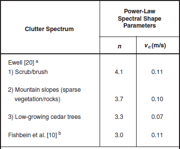
aSpectral shape parameters shown are valid for approximating clutter spectra over ac spectral dynamic ranges reaching ∼40 to 45 dB down from the zero-Doppler peak.
bValid to ∼ 35 dB down
Also included for comparison in Table 6.6 are Fishbein et al.’s original power-law spectral shape parameters. The Fishbein et al. power law is wider than the three desert power laws in Table 6.6 (e.g., the Fishbein et al. power law reaches the −30-dB level at v = 1.7 m/s), although part of the reason for the wider Fishbein et al. data is that they were noncoherent. Besides corroborating gross spectral extents of Phase One and LCE clutter spectra measured at upper ranges of spectral power under breezy conditions, the results of Ewell’s spectral measurements shown in Table 6.6 also tend to substantiate the Phase One and LCE findings that ac clutter spectral shape, at least to first-order, tends to be approximately independent of terrain type and that clutter spectral shape tends to be largely independent of polarization.
Status (Power-Law Spectral Shape). Many measurements of windblown clutter spectra obtained following the very early measurements of Barlow and others provide spectral dynamic ranges typically reaching ∼ 30 or ∼ 40 dB below zero-Doppler peaks. Such measurements, as reviewed in the preceding discussion, provide clutter spectral shapes that are frequently well represented as power laws.
In contrast to the Gaussian spectral shape which theoretically arises from a random group of scatterers each of constant translational drift velocity, there is no simple physical model or fundamental underlying reason requiring clutter spectral shapes to be power law. All theoretical investigations of clutter spectra based on physical models that include oscillation and/or rotation in addition to translation of clutter elements provide expressions for clutter spectra that are to greater or lesser degree of complex mathematical form [14, 18, 29, 39, 54, 55], although one such expression [14] is derived to be a negative power series in f (i.e., as a sum of elemental power laws) which at least does have a general power law-like behavior.
Because the preponderance of the empirical evidence in spectral measurements to levels 30 or 40 dB down from zero-Doppler peaks has been for simple power-law spectral shapes, there has been some motivation by theoreticians either to reduce an initially derived complex formulation for clutter spectral shape to a simpler, approximately power-law formulation [18] or to show that numerical evaluation of the complex formulation provides results that closely match a simple power law [19]. However, the evidence that clutter spectra have power-law shapes over spectral dynamic ranges reaching 30 to 40 dB below zero-Doppler peaks is essentially empirical, not theoretical.
6.6.1.3 EXPONENTIAL SPECTRAL SHAPE
Phase One and LCE ground clutter spectral measurements to levels 60 to 80 dB down indicate that the shapes of the spectra decay at rates often close to exponential [21, 25]. The two-sided exponential spectral shape is given by Eq. (6.2), repeated here as:
where β is the exponential shape parameter, K = β/2 is the normalization constant, k(v) = exp (–β|v|), and
To convert to Pac(f) in Eq. (6.2), i.e., Pac(f)df = Pac(v) dv, replace v by f and β by (λ/2)β. The standard deviation of the exponential spectrum of Eq. (6.2) is given by ![]() in units of m/s. The exponential shape is wider than Gaussian, but in the limit much narrower than power law whatever the value of the power-law exponent n. Like the Gaussian, the exponential is simple and analytically tractable. For example, the Fourier transform of the exponential function is a power-law function of power-law exponent n = 2 [8, 51]. The exponential shape is easy to observe as a linear relationship in a plot of 10 log Pac vs v. Figure 6.21 shows four cases of measured Phase One and LCE spectra that are remarkably close to exponential over most of their Doppler extents, and other examples of Phase One and LCE exponential or quasi-exponential clutter spectral decay are provided elsewhere in Chapter 6. There is no known underlying fundamental physical principle requiring clutter spectra to be of exponential shape. Rather, the exponential shape is a convenient analytic envelope approximating the shapes of many of the Phase One and LCE measurements to levels 60 to 80 dB down.
in units of m/s. The exponential shape is wider than Gaussian, but in the limit much narrower than power law whatever the value of the power-law exponent n. Like the Gaussian, the exponential is simple and analytically tractable. For example, the Fourier transform of the exponential function is a power-law function of power-law exponent n = 2 [8, 51]. The exponential shape is easy to observe as a linear relationship in a plot of 10 log Pac vs v. Figure 6.21 shows four cases of measured Phase One and LCE spectra that are remarkably close to exponential over most of their Doppler extents, and other examples of Phase One and LCE exponential or quasi-exponential clutter spectral decay are provided elsewhere in Chapter 6. There is no known underlying fundamental physical principle requiring clutter spectra to be of exponential shape. Rather, the exponential shape is a convenient analytic envelope approximating the shapes of many of the Phase One and LCE measurements to levels 60 to 80 dB down.
In Eq. (6.2), the independent variable v may itself be raised to a power, say n, as: exp (–β|v|n) to provide an additional degree of freedom in curve-fitting to measured data. When n > 1, this results in convex-from-above spectral shapes on 10 log P vs v axes, that is, in shapes that decay faster than exponential (e.g., when n = 2 the shape becomes Gaussian). On the other hand, n < 1 (i.e., fractional) results in concave-from-above spectral shapes on 10 log P vs v axes, which is the direction away from purely exponential that measured Phase One and LCE spectra usually tend towards, especially at lower wind speeds. Provision of a more complex exponential-like expression to possibly enable improved curve-fitting capability to particular empirical data sets is not further pursued here since the simple exponential form (i.e., n = 1) satisfactorily captures the general shapes and trends in the data.
The Phase One clutter data were shared with the Canadian government. Chan of Defence Research Establishment Ottawa (DREO) issued a report [22] and subsequent paper [23] on the spectral characteristics of ground clutter as determined largely from his investigations of the Phase One data, but also including measured ground clutter spectra from a DREO rooftop S-band phased-array radar. Figure 6.52 shows some of Chan’s results comparing clutter spectra from the same two resolution cells under windy and breezy conditions. In the main, Chan’s results agree with those of Lincoln Laboratory. In arriving at these results, Chan used a different set of the Phase One data than the long-time-dwell experiments used at Lincoln Laboratory in spectral processing. That is, to obtain a larger set of measurements, Chan used repeat sector Phase One data (see Chapter 3) which provided more spatial cells but shorter dwells, and performed maximum entropy spectral estimation on these data to obtain the necessary spectral resolution. Thus with different data, different processing, and, in the case of the DREO phased-array instrumentation, a different radar, Chan also arrived at exponential spectral decay for what he calls the “slow-diffuse” component of the ground clutter spectrum. Indeed, the spectra from the DREO radar shown in Figure 6.52 appear for the most part to be highly exponential in spectral shape. Stewart [43] has also shown a measured ground clutter spectral shape of relatively wide spectral extent that appears highly exponential.
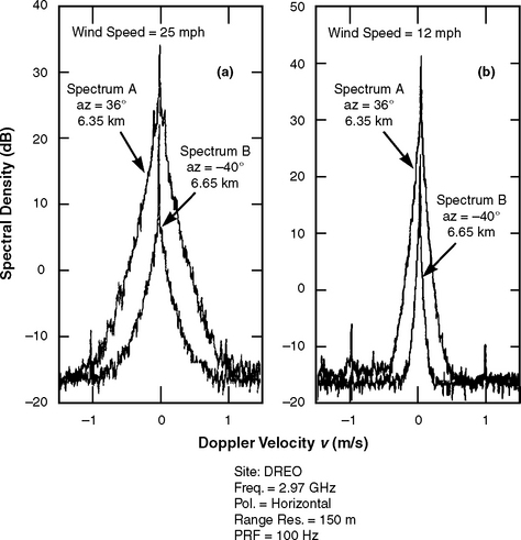
FIGURE 6.52 Measurements of radar ground clutter power spectra by Chan of DREO (Canada) showing results from the same two resolution cells under windy conditions (a), and breezy conditions (b). After [22], 1989.
The empirical observations of exponential decay in the Phase One and LCE clutter spectra motivated White [39] to develop a new first-principles physical model for radar backscatter from moving vegetation that also provides exponential spectral decay to conform in this respect with the experimental evidence. White’s model assumes that an important element of the scattering arises from the tree branches. The key feature of the model is the representation of each branch as a cantilever beam clamped at one end. Distributions of branch lengths is Gaussian. Distribution of branch angles with respect to horizontal is uniform over π radians. Scattering centers are distributed uniformly over an outer (specifiable) portion of each branch. A mathematical expression for the Doppler spectrum of the radar return from such an assemblage of branches under a distributed wind forcing function is derived. This expression is a complex five-part multiple integral requiring numerical evaluation. When numerically evaluated, the resultant Doppler spectrum is shown to very closely provide exponential decay with increasing Doppler frequency.
In addition, the sensitivity of White’s exponential spectral shape to a number of his model assumptions was tested numerically. It was found that the exponential shape was not very sensitive to a number of underlying assumptions concerning the beam modes of oscillation, but much faster than exponential decay occurred when the beams were not clamped (i.e., simple translation), when a nondistributed wind force was used, and when branch lengths were uniformly (as opposed to Gaussianly) distributed. Besides this exponential spectral component arising from branch motion, the model also postulates a rectangular wideband background spectral component at lower power levels arising from leaf motion (see Section 6.6.3.3). Although White’s main thrust was the development of a theoretical clutter spectral model, he also provided a small amount of measured radar clutter spectral data acquired using a rooftop C-band radar of spectral dynamic range reaching ≈30 to 40 dB below zero-Doppler peaks. White concluded from curve-fitting studies comparing power-law with exponential approximations to his measured data that “… the exponential model is the better fit” [39].
Using a different method of analysis than that of White, Lombardo [60] presents a mathematical formulation for ground clutter spectral shape derived from a phenomenologically representative negative binomial probability distribution of scatterer velocities that also can yield an exponential decay characteristic in the tail.
Measured results very similar to those of Phase One and LCE but over less wide, 40- to 60-dB dynamic ranges were obtained in a much earlier set of Lincoln Laboratory measurements of ground clutter spectra at UHF and L-band [59]. Clutter spectra from this earlier program averaged over a number (e.g., 5) of range cells and displayed on log-Doppler velocity axes typically show an increasing rate of downward curvature (convex from above) as in the LCE and Phase One measurements. By coincidence, this early Lincoln Laboratory program [59] of 1972 and the Russian X-band investigations [13] going forward in very nearly the same time period (1973) both developed first-principles physical models of clutter spectra from forest. In both studies, the tree was modeled as a mechanical resonator excited by a turbulent wind field of known spectral content. Both programs involved measurements of tree motion. In both programs, the spectral content of tree motion decayed at low frequencies below a resonance maximum according to an n = 5/3 power law; at higher frequencies above the resonance maximum, the decay was faster. The slightly later (1974), largely theoretical paper by Lincoln Laboratory authors [55] concerning electromagnetic scattering from vegetative regions included three measured clutter spectra from the 1972-era measurement program.
Shoulders before the onset of faster decay, such as those shown in some of the LCE- and Phase One-measured clutter spectra (e.g., see Figures 6.22, 6.24, and 6.25), are similar to those observed previously in the earlier Lincoln Laboratory program [59] and explained as local resonance maxima associated with the natural resonant frequency of trees. The resonance shoulder was more pronounced at lower frequencies and lower wind speeds, and tended to diminish at higher frequencies and higher wind speeds. The reason is that, at lower wind speeds and longer wavelengths, the motion of the tree is a small fraction of a radar wavelength. Thus under these conditions the tree motion superimposes a phase modulation with low index of modulation, and as a result the clutter spectrum directly corresponds with that of the tree’s physical motion. At higher frequencies and under stronger winds, the degree of phase modulation increases and the clutter spectrum no longer simply replicates that of the tree motion. These observations tend to be corroborated in LCE and Phase One results. In addition, the LCE and Phase One data tend to have resonance shoulders to somewhat higher frequencies in measurements from partially open or open terrain (desert, farmland, rangeland) in which there is a significant dc component; the measurements from forested terrain tend to have distinct resonance shoulders only at the lower radar frequencies (VHF and UHF). The earlier Lincoln Laboratory program observed, in passing, that the shapes of some measured spectra beyond the resonance shoulder were highly exponential, but this observation was not elaborated upon.
Another early, more explicit, observation of exponential spectral shape is in the results of Andrianov, Armand, and Kibardina [16] (see Figure 6.50). In these results, exponential decay was initially observed from the maximum zero-Doppler level down to −20 dB, followed by power-law decay thereafter to −70 dB with reported values of n equal to 3.4, 3.8, and 5.6 for pine, alder, and birch, respectively. The equipment used was ostensibly of 70-dB dynamic range [15] although, to use their words translated to English, two dynamic range intervals were “sewn together” [16], as shown in Figure 6.49, to provide the full 70-dB range. In terms of gross spectral extent (e.g., 1.5 m/s, 70 dB down; 0.4 m/s, 20 dB down), these results of Andrianov et al. [15, 16] fall closely within the range of measured LCE and Phase One spectral extents over similar spectral dynamic ranges. The earlier results of Kapitanov, Mel’nichuk, and Chernikov [13], as shown in Figure 6.48, were said to exhibit Gaussian decay down 10 to 15 dB, followed by power-law decay with n = 4 down to −40 dB. The initial Gaussian decay was later stated to be erroneous by Andrianov et al. [16] because of early equipment limitations and that initial exponential decay as reported by them (see Figure 6.50) was more correct.
The exponent n of the power law is easy to estimate in measured spectral data as simply one-tenth the slope of the approximating straight line on 10 log P vs log v axes in dB/decade. In Figure 6.50, the three measured spectral curves for pine, alder, and birch shown to the left do not exhibit decay anything like the quoted power-law slopes of n = 3.4, 3.8, and 5.6, respectively. These three curves are stated by the authors to be three particular examples of measured spectra, whereas their quoted values of n are averages over all measurements in which the value of n varies from 2.6 to 6.8. The rates of decay in the spectral tails of the data to the left in Figure 6.50 are much greater than any of these quoted values of n and, at least in qualitative appearance (increasing downward curvature), appear to be more exponential than power law. The data of Figure 6.49 appear to be more credibly of power-law behavior (n ≈6) in their tails, but the data plotted at the −68-dB level indicate slightly increasing curvature (rate of decay > n ≈6) at the lowest power levels shown. The data of Figure 6.48 closely match the n = 4 power law attributed by the authors to these data.
Some confusion may arise because these Russian investigators [13–16] associate power-law shapes with lower ranges of spectral power in their measured data, whereas other investigators [10–12, 17–20] match their data to power-law shapes over upper ranges of spectral power. Measured clutter data in any particular regime of spectral power may be fitted with a power law, but the danger lies in extrapolating the power law beyond its regime of applicability.
An additional, somewhat more significant, past use of the exponential function to characterize clutter spectra from windblown vegetation occurred in experimental work performed at the Laboratoire Central de Telecommunications in France [38]. These French measurements were also performed during the 1970s using coherent-on-receive radars, spectrum analyzers with limited (i.e., 50 dB) dynamic range, and a limited number of vegetation clutter types. In this work, the MTI filter cutoff frequency was adjusted so as to be just sufficient to remove the clutter to the −40-dB level. It was found that the cutoff frequency just sufficient to remove the clutter was best predicted by hypothesizing an exponential spectral clutter model. The cutoff frequency predicted by a Gaussian spectral model was too low (i.e., optimistic—if there was even a light wind, significant clutter was passed by the filter); whereas the cutoff frequency predicted by a power-law spectral model was too high (i.e., pessimistic—at X-band, all targets with radial speed < 50 km/h were missed). In contrast, cutoff frequencies in the range predicted by an exponential spectral model were successfully used as the standard specification for many service radars in the French military and elsewhere.
Status (Exponential Spectral Shape). The significantly increasing rate of downward curvature (i.e., convex from above) observed in the general shapes of Phase One- and LCE-measured windblown ground clutter Doppler spectra on 10 log P vs log v axes over spectral dynamic ranges reaching 60 to 80 dB below zero-Doppler peaks points to a general exponential characterization rather than a power-law characterization that plots linearly on such axes. Increasing rate of downward curvature in such plots has always been observed without exception in all measurements examined of clutter spectra from windblown trees and other vegetation under breezy or windy conditions taken from these extensive databases. Other investigators [22, 24] have corroborated that the exponential shape factor is generally representative of these data and is not the result of processing-specific particulars.
In early studies, theoretical investigators attempted to reduce complex mathematical formulations of clutter spectra based on physical models incorporating oscillation and/or shadowing of elemental scatterers to simple power-law forms to conform with the experimental evidence then available at upper levels of spectral power (down 30 or 40 dB from zero-Doppler peaks). Subsequent awareness of investigators of the Lincoln Laboratory clutter spectral results provided motivation to develop theoretical bases for the observed exponential spectral shapes. Thus there exist the interesting works of White [39] and Lombardo [60] in which formulations are developed for the clutter Doppler spectrum, that, although mathematically complex, provide close to exponential decay under numerical evaluation. In addition, White observed that “the series solutions produced by Bass et al. [54], Armand et al. [14], and Wong et al. [29] probably have sufficient degrees of freedom to produce a function that would be a close approximation to … exponential …” [39]. Nevertheless, as for the power law for spectral dynamic ranges 30 to 40 dB down, the evidence of exponential clutter spectral shape for spectral dynamic ranges reaching 60 to 80 dB down is essentially empirical.
The only known measurements of windblown clutter spectra of spectral dynamic ranges equal to or exceeding those of the Phase One and LCE instruments are the Russian measurements of the 1970s [13–16], for which the results over lower ranges of spectral power were approximated as power laws. However, these results are power law only in a piece-part sense; the upper range of spectral power was concluded to be exponential. Hence these results are not very useful or analytically tractable, in that no single simple analytic function was provided to describe the complete clutter spectral shape over its full measured spectral dynamic range. Furthermore, little actual measurement data were shown in these papers, thus restricting possibilities for independent assessment of the data and conclusions by present-day readers.
Like the Gaussian function, the exponential function is simple and analytically tractable. The exponential function provides spectral shapes that are wider than Gaussian, as required by all the empirical evidence and by theoretical constructs involving oscillation, rotation, and shadowing of clutter elements; that are very much narrower at lower power levels (60 to 80 dB down) than extrapolations to lower levels of power-law representations of measurements accurate at higher levels of spectral power (30 to 40 dB down); and that are reasonably equivalent to the measurement data at high and low levels of spectral power.
6.6.2 RECONCILIATION OF EXPONENTIAL SHAPE WITH HISTORICAL RESULTS
6.6.2.1 Current vs Historical Clutter Spectral Measurements
Figure 6.5 (Section 6.3.2.1) shows a measured LCE clutter spectrum from windblown trees and compares it with several exponential shape functions (dotted lines) of various values of exponential shape parameter β. In Figure 6.5, the measured data closely follow the exponential curve of shape parameter β = 5.2 over the full spectral dynamic range shown. Also shown in Figure 6.5 is a narrower Gaussian spectral shape function (dashed line) corresponding to Barlow’s much-referenced historical measurement [7] (see Figure 6.45). The Gaussian curve in the figure is shown extrapolated to low spectral power levels much below Barlow’s measured spectral dynamic range, which reached only 20 dB below the zero-Doppler peak. The overall rate of decay in the LCE data of Figure 6.5 is much more exponential than Gaussian in character. Spectral tails wider than Gaussian are theoretically required by branches and leaves in oscillatory motion [19, 29] (see Section 6.6.1).
Figure 6.53 shows another LCE windblown-tree clutter spectrum different from that of Figure 6.5. The spectrum of Figure 6.53 was measured at vertical polarization on 11
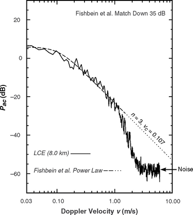
FIGURE 6.53 Comparison of an LCE windblown forest clutter spectrum with the Fishbein et al. power-law model [10].
September at Wachusett Mt. at range = 8.0 km. Also shown in the figure is the n = 3, vc = 0.107 power-law curve introduced by Fishbein et al. [10] to match their data (Figure 6.46). This Fishbein et al. power-law curve is shown dashed in Figure 6.53 to a level 35 dB down from the zero-Doppler peak, which is the region for which Fishbein et al. had data; at lower levels in Figure 6.53 the Fishbein et al. power-law curve is shown dotted to indicate extrapolation to levels below Fishbein et al.’s noise floor. The LCE data in Figure 6.53 provide a remarkably close match to the Fishbein et al. power-law curve at upper levels (viz., down 35 dB) over which Fishbein et al. had data. That is, these LCE spectral data confirm the historic Fishbein et al. spectral measurement with modern measurement instrumentation. However, it is also very clear in Figure 6.53 that the Fishbein et al. power-law curve cannot be extrapolated to lower levels. At lower levels, the LCE measured spectrum in this figure decays much more rapidly than at upper levels. In overall shape, the LCE data of Figure 6.53 are not very different from Figure 6.5 and are better modeled as exponential over their complete range than as any power law.
The Fishbein et al. measurement (Figure 6.46) was made with noncoherent instrumentation; thus the Fishbein et al. power-law approximation shown in Figure 6.53 is ∼1.4 times wider than would be expected if the measurement had been coherent (see Section 6.6.1.1; the 1.4 factor is specifically applicable to spectra of Gaussian shape, but a similar factor is expected to apply to spectra of power-law shape). The LCE coherent measurement shown in Figure 6.53, although of similar relative shape to what would be expected if Fishbein et al. had made a coherent measurement, is thus wider in absolute terms at upper power levels (> −35 dB) than what would be expected in such a measurement. Even so, the narrower Fishbein et al. coherent measurement, if modeled as an n = 3 power law, would still extrapolate at lower levels (< −35 dB) to spectral extents much broader than any LCE measurement at these lower levels, including LCE narrower measurements selected to match the coherent Fishbein et al. measurement at upper power levels.
Figure 6.21 (Section 6.4.2) shows measured LCE and Phase One clutter spectra as 10 log Ptot vs v from cells containing windblown trees on breezy and windy days. These results are among the widest windblown clutter spectra measured by these instruments. In contrast with most of the other historical spectral measurements discussed in Section 6.6.1, the measurements of Figure 6.21 over greater spectral dynamic ranges than were available in most of the other measurements have spectral shapes that are accurately representable as exponential. This accurate exponential representation is indicated by the good fits of the data to the straight lines drawn through the right sides of the spectra in Figure 6.21.
Figure 6.54 shows the right sides of Figures 6.21(a), (b), respectively, plotted as 10 log Ptot vs log v. Recall that the power-law spectral shape [Eq. (6.18)] plots as a straight line in the spectral tail region v >> vc using a log-Doppler velocity axis as in Figure 6.54. Certainly no single power-law straight line fits either of the spectral data traces in Figure 6.54, both of which exhibit strong downward curvature (convex from above) over their complete spectral extents. Even though the measurement data in Figure 6.54 exhibit strong downward curvature, a local power-law rate of decay can be defined for such data in a small Doppler interval δv as the value of power-law exponent n corresponding to the slope of the straight line tangent to the data curve in the region δv. The local power laws that thus fit the upper levels over historic dynamic range intervals in Figure 6.54 (n = 3 or 3.5) cannot be extrapolated to lower levels. Much faster decaying local power laws (n = 7, 8, or 10.5) fit the lower levels.
In both Figures 6.53 and 6.54, the more sensitive Phase One and LCE measurement instruments confirm measured rates of spectral power decay reported by other investigators at upper power levels, but in addition find that much faster local power-law rates of decay occur at lower power levels. Close examination of the spectral data in Figures 6.53 and 6.54 appear to indicate, in fact, two or more distinct rates of decay in the spectra, perhaps indicating different phenomenological regimes with different sets of scatterers and/or different mechanisms of scatter dominating at different spectral power levels. On the basis of these results, it is not surprising that many previous investigators have characterized the rate of ground clutter spectral decay at relatively high spectral power levels (i.e., 35 to 45 dB down) as n = 3 or n = 4 power laws.
In Figure 6.54, exponential fits to the data are shown lightly dotted. The exponential shape β = 7.1 closely fits the Phase One data of Figure 6.54(b) over its full ac spectral range away from its quasi-dc region (i.e., |v| > ≈0.2 m/s), including both regions of local power-law fits; similarly, the exponential shape β = 5.2 closely fits the LCE data of Figure 6.54(a) over its full ac range (i.e., |v| > ≈0.1 m/s). In Figure 6.44, the exponential β = 6 curve lying between Barlow’s g = 20 Gaussian curve and the Fishbein et al. n = 3 power-law curve is now seen as reasonably representative of the data shown in Figure 6.54 from two different instruments at two different sites across more than six orders of magnitude of diminishing spectral power.
6.6.2.2 MATCHING MEASURED CLUTTER SPECTRA WITH ANALYTIC SHAPES
Figure 6.55 compares the β = 6 exponential shape with vc = 0.1; n = 3, 4, 5 power-law shapes both on 10 log P vs v axes [Figure 6.55(a)] and on 10 log P vs log v axes [Figure 6.55(b)]. Each of the four spectral shapes shown is normalized to equivalent unit spectral power as per Eqs. (6.2) and (6.18). Figure 6.55(a) uses a linear Doppler velocity axis, making evident how all power-law shapes become slowly decaying at low levels of spectral power, whatever the value of n. Given that the maximum Doppler velocities observed in Phase One- and LCE-measured clutter spectra were in the 3- to 4-m/s range at levels 60 to 80 dB down, the power-law parameters vc and n can certainly be adjusted to provide similar spectral extents at similar power levels. However, the resultant power-law shapes will not match Phase One- and LCE-measured data at higher levels of spectral power and will rapidly extrapolate to excessive spectral width at lower levels.
As plotted against the logarithmic Doppler velocity axis in Figure 6.55(b), the β = 6 exponential shape demonstrates the increasing downward curvature (convex from above) with increasing Doppler velocity and decreasing power level that characterizes all the Phase One- and LCE-measured clutter spectra when plotted on such axes. In contrast, the power-law shapes in Figure 6.55(b) have little curvature. That is, on 10 log P vs log v axes, power-law shapes are asymptotic to two straight lines with a maximum departure in curvature below these asymptotes of only 3 dB at the v = vc breakpoint between them. This rapid rotation from near-horizontal to straight line spectral tails in which rapidly increasing downward curvature is constrained to a very narrow v = vc Doppler regime is not generally characteristic of the Phase One- and LCE-measured clutter spectral shapes.
6.6.2.3 SUMMARY
The Phase One and LCE measurements of ground clutter spectra presented in Chapter 6 are displayed on both linear and logarithmic Doppler velocity axes. What is clear in these presentations, and what has not been generally recognized, is that if the clutter ac spectral shape Pac is represented as a power law, the power-law exponent n is not constant but gradually increases from n = 3 or 4 when Pac is 35 or 40 dB down from its maximum to n = 5 or 6 or even higher when Pac is 60 to 80 dB down from its maximum. Uncertainty about whether “the law” of spectral decay is “n = 3 or n = 6 (or even exponential)” is abetted by the additional lack of general recognition that the shape of the spectrum to levels 60 to 80 dB down is usually not precisely representable by any single analytic expression. In the results presented herein, slight upward curvature (concave from above) often occurs on the 10 log Pac vs v plots, hence the shape can be slightly broader than exponential; whereas strong downward curvature (convex from above) almost always occurs on the 10 log Pac vs log v plots, hence the shape is much narrower than constant power law.
Thus there is no argument with Andrianov, Armand, and Kibardina that “It is [usually] impossible to [precisely match] the spectral density of the scattered signal by a single analytical function in the entire range of [Doppler] frequencies” [16]. However, much of the potentially ensuing difficulty in the general modeling of clutter spectra is overcome in Chapter 6 not just by utilizing exponential shapes, but also by introducing the concept of a quasi-dc region and absorbing excess power in this region into the dc delta function term of the model (see also [31]). However the spectrum is modeled, the Phase One and LCE results support the general existence of windblown clutter Doppler velocities only as great as ∼ 3 to 4 m/s for 15- to 30-mph winds to levels 70 to 80 dB down.
The evidence for both power-law and exponential clutter spectral shapes is essentially empirical. The concern in Chapter 6 is not which of these two forms fits the data best over spectral dynamic ranges of −30 or −40 dB, or even whether such a question can be definitively answered. Chapter 6 provides good examples of both power-law and exponential fits to measured clutter spectral data to levels 30 or 40 dB down, and in reviewing the technical literature finds it to be similarly bipartite on this matter. The concern is, however, in determining an appropriate functional form to describe clutter spectra over greater spectral dynamic ranges. The main observation in this regard, based on the Phase One and LCE databases, is that no matter how good the power-law fits are over spectral dynamic ranges extending 30 to 40 dB below zero-Doppler peaks, they cannot be extrapolated to lower levels. That is, power-law shapes extrapolate rapidly to excessive spectral width. In contrast, the exponential form generally represents the Phase One and LCE measurements not only over their upper ranges of spectral power but also over their complete spectral dynamic ranges extending to levels 60 to 80 dB below zero-Doppler peaks. Thus radar system design for which ground clutter interference is of consequence at such low levels of spectral power is much more accurately based on an exponential clutter spectral shape approximation than on an extrapolated power-law approximation. The validity of the exponential shape on the basis of best matching coherent detection system performance to that obtained using actual measured I/Q clutter data as input to the clutter processor is demonstrated in Section 6.5.4.
6.6.3 REPORTS OF UNUSUALLY LONG SPECTRAL TAILS
Several historical reports of spectral tails in ground clutter at unusually high power levels and/or extending to unusually high Doppler velocities are considered in the following subsections.
6.6.3.1 TOTAL ENVIRONMENT CLUTTER
There exists significant concern with how to characterize the clutter residues left in Doppler filter banks in high sensitivity radars after MTI cancellation that might cause false targets for subsequent multitarget tracking algorithms. Thus there is interest in specifying an overall environment clutter model that would include the Doppler interference from such things as aurora, meteor trails, cosmic noise, windblown material (leaves, dust, spray), birds and insects, rotating structures, rain and other precipitation, lightning, clear air turbulence, fluctuations of refractive index, etc. Often such phenomena are highly transient as they occur in measurements of radar Doppler spectra, so that it is difficult to causally and quantitatively associate unusual spectral artifacts directly with their sources. It is not suggested here that a specific program dedicated to measuring any one of these phenomena would not be successful—rather, that in a general database of spectral measurements collected from spatial ensembles of remote ground clutter cells, the occasional occurrence of causative agents different from windblown vegetation is difficult to determine. The main focus of interest in the Phase One and LCE spectral measurements is the general and continuous spectral spreading that occurs in ground clutter due to wind-induced motion of tree foliage and branches or other vegetative land cover. These clutter databases have not been very extensively used for systematic searching for infrequent, spatially unusual, narrowband, or transient spectral features resulting from other causative agents in the total clutter environment because of their ephemeral nature and uncertain signature characteristics, although occasional evidence of birds, airplanes, automobiles, and other anomalies has been encountered in the spectral analyses of these data. The one concrete example encountered by the LCE radar of clutter from the total environment over land with atypical spectral behavior was strong Bragg resonance at small, but nonzero Doppler frequencies in the returns from a small inland body of water [34, 35]. Some of the unusually long spectral tails attributed to windblown clutter in the following discussions may have originated from external sources other than windblown vegetation or from internal instrumentation or data processing effects of which the investigators were unaware.
6.6.3.2 CHAN’S “FAST-DIFFUSE” COMPONENT
In addition to a “slow-diffuse” exponential component in ground clutter spectra, Chan [22, 23] also introduced a “fast-diffuse” component at a relatively weak but constant power level out to a higher Doppler frequency cutoff than the slow-diffuse component. Both components are indicated in Chan’s idealized diagram of a composite ground clutter model shown in Figure 6.56. The fast-diffuse component is based on the observation of very infrequent or narrowband spectral features usually observed in isolated cells and for short-duration time intervals. The amplitude and cutoff frequency of the fast-diffuse component are not specified by Chan; however, for all his fast-diffuse examples, the maximum, or cutoff Doppler velocity, although greater than the slow-diffuse component present, was ≤ 2.5 m/s. Such occasional spectral features may often be caused by total environment clutter (birds, etc.).

FIGURE 6.56 Chan’s conceptual composite clutter model, including a fast-diffuse component. From [22], 1989. See also [23].
Transient, isolated, narrowband spectral features at low Doppler that do not exist symmetrically to either side of zero-Doppler can often, with some degree of confidence, be attributed to birds. Chan speculated that “regular oscillatory motion of [crop] vegetation, arising from restricted freedom of travel and natural elasticity” [22] might explain some unusual symmetrical features. Similar features have not been observed at Lincoln Laboratory, although Chan was using different Phase One data (repeat sector) and different processing (maximum entropy). Nonlinear superresolution processing techniques (such as maximum entropy) usually require large S/N ratios—not available at low levels in measured clutter spectra—to avoid spurious results. Spectral contaminants from the measurement instrument or from external RF sources of interference may also be present.
Spectral features that are not isolated but exist in all spatial resolution cells, and/or that exist symmetrically to either side of zero-Doppler, are likely to be instrumentation or processing contaminants.
Probabilities of occurrence, which would be difficult to determine, would eventually be required in a model for fast-diffuse spectral features. In any event, experience has indicated that Chan’s fast-diffuse spectral component is easily misunderstood to imply the existence of a long, continuous, low-level, uniform amplitude spectral tail in ground clutter that is always there for all cells and all times. In fact, the fast-diffuse component was based on the observation of infrequent spectral artifacts.
6.6.3.3 WHITE’S WIDEBAND BACKGROUND COMPONENT
White’s physical model [39] for windblown trees, which provides an exponential spectral component, also provides a rectangular wideband background spectral component at lower power levels. White essentially postulated the existence of his background component on the basis of Chan’s fast-diffuse component [22, 23]. In so doing, White—as others have done—appears to have misinterpreted Chan’s fast-diffuse component in the manner discussed above. Thus, whereas Chan’s fast-diffuse component was based on the observation of infrequent spectral artifacts out to a maximum observed Doppler velocity of 2.5 m/s, White took this as the basis for postulating a wideband noise-like spectral component with “… a uniform spread of spectral power over all [Doppler] frequencies up to about 1 kHz” [39]. A cutoff frequency of 1 kHz corresponds to Doppler velocities of 15 and 50 m/s for the X- and S-band radars, respectively, that White was considering, which is well beyond Chan’s observed cutoff.
White provided heuristic argument for the existence of a wideband background spectral component based on leaf (as opposed to branch) motion. In particular, he argued that rapid decorrelation in the returned signal resulting from the shadowing of one leaf by another and by leaf rotation can be expected to give rise to a wideband noise component. White did not derive a mathematical expression for the wideband component, and its absolute level was not specified.
White attempted to provide some experimental evidence for the wideband background spectral component in his limited set of C-band measured ground clutter data. This experimental evidence is unconvincing. The spectral dynamic range of the measurement radar was not shown or specified, but it was stated that the radar had a “… reasonably high radar noise floor” [39]. Results were provided for a quiet day and a windy day. In both sets of results, what was claimed to be the wideband background component also has the appearance of a system or processing noise floor. In both sets of results, cells with significantly spread clutter spectra, cells with little, and cells with no clutter Doppler spread were separately combined to provide averaged clutter spectra with wide, some, and no clutter spread.
It was observed that the noise-like background component was somewhat higher in spectral power level for the wide averaged spectrum than for the other two averaged spectra with little or no spread. In the quiet-day results, this difference in background level was small, and it was concluded that “the apparent white noise component … is due to … Fourier sidelobes and system noise” [39]. In the windy-day results, the difference was somewhat greater. It was argued that in this case this difference indicates “a real white-noise scatterer motion within the band limits of the radar” [39]. In White’s plotted results, what was claimed to be the white-noise spectral component occurs about 38 dB below the zero-Doppler peak.
The Phase One and LCE databases of clutter spectral measurements provide no evidence for the existence of a noise-like wideband background spectral component within the spectral dynamic ranges of these instruments, which reach 60 to 80 dB below the zero-Doppler spectral peaks. The Armand et al. [14] measured clutter spectral data (discussed subsequently in Section 6.6.3.6) at 4-mph wind speed show a noise-like component at a constant level of ∼ −115 dB extending over the range 2.5 < v < 20 m/s. At the higher wind speeds of 13 and 31 mph, the Armand et al. data decay continuously and reach the −115-dB level only at the limit of the measured data as v reaches ∼20 m/s. No convincing evidence is provided by Armand et al. that the −115-dB level in these data is not a noise level. The bare-hill data of Warden and Wyndham [11] show a hint of a possible constant noise-like tail beginning at the −24-dB level (0.55 < v < 0.65 m/s), which is almost certainly a noise level or other corruptive influence (see Figure 6.47). In a private communication, White agreed that some degree of skepticism was warranted concerning his postulated wideband noise-like background component [61].
6.6.3.4 SIMKINS’ “LOWLAND” DATA OF WIDE SPECTRAL EXTENT
This discussion concerns the L-band measurements of clutter spectra by Simkins, Vannicola, and Ryan [17] shown in Figure 6.51. Modeling information for spectral shape derived from these measurements was based on upper-bound approximations to worst-case spectra. These worst-case spectra came from resolution cells causing false alarms in a three-pulse-canceller MTI channel. These cells causing false alarms led to v−3 and v−4 power-law estimates of spectral shape. Spectra from adjacent cells with similar intensity but which did not cause false alarms were narrower, with v−5 or exponential shape.
Relative frequencies of occurrence of false alarm cells compared with non-false alarm cells were not specified. False alarms can be caused by transient events in the total clutter environment other than generally pervasive windblown vegetation. False alarms that moved measurable distances over several PPI scans were called angels; possible associations of angels, primarily with birds, but also with insects, clear air turbulence, and aurora, were discussed. Other false alarms were due to anomalous propagation, for which no spectral data were taken. Stationary false alarm cells were assumed to be caused directly by area-extensive ground clutter (as opposed to having less direct total environment origins) and used to develop ground clutter spectral modeling information.
Consider first the Simkins et al. ground clutter spectral data for “partially wooded hills” in 10- to 20-knot winds. The v−4 power-law shape attributed to these data in Figure 6.51 is an approximate upper-bound to an underlying scatter plot of data points. These data points, as typified by ≈–30 dB at 0.25 m/s and ≈–40 dB at 0.5 m/s, are not out of line with Phase One and LCE data. It is not the characterization of the bounding shape of these data as v−4 over the indicated 45-dB dynamic range that leads to difficulty, but the extrapolation of a constant v−4 power-law shape to power density levels significantly lower than −45 dB. Phase One and LCE also often show v−3 and v−4 rates of decay 35 to 40 dB down, but these become v−5 and v−6 rates of decay 60 to 80 dB down.
Consider next the Simkins et al. ground clutter spectral data for “heavily wooded valleys” or “lowlands” in 10- to 20-knot winds also shown in Figure 6.51. A wider v−3 power-law shape was attributed as an upper bound approximation to these data. These heavily-wooded-valley data, as typified by ∼ −7 dB at 0.5 m/s and ∼ −15 dB at 1 m/s, are significantly wider than Phase One- and LCE-measured spectra (the widest LCE spectrum is ∼ −20 dB at 0.5 m/s and ∼ −30 dB at 1 m/s). The maximum measured Doppler velocity among the heavily-wooded-valley spectral data points is 5.8 m/s, 40 dB down; 5.8 m/s is almost twice the maximum Doppler velocity of ∼ 3 m/s for windblown trees consistently seen by LCE in 15- to 30-mph winds, 70 to 80 dB down, and almost four times the Doppler velocity of 1.5 m/s seen in the widest LCE spectrum, 40 dB down. No other known measurement of a ground clutter spectrum approaches such high spectral power at such high Doppler velocity as given by the 5.8 m/s, −40-dB point of the Simkins et al. heavily-wooded-valley data.
On the basis of the many Phase One and LCE results in 15- to 30-mph winds, attributing Doppler velocities of 5.8 m/s, 40 dB down, to windblown trees would conjecturally require wind velocities much greater than the nominal 10 to 20 knots associated with the heavily-wooded-valley data. The only other known measurements of ground clutter spectra in which spectral power decays as slowly with increasing Doppler velocity as in the Simkins et al. heavily-wooded-valley data are early results reported by Goldstein [9] for trees in gale-force winds, discussed next in Section 6.6.3.5; however, these measurements only extend to a maximum Doppler velocity of 1 m/s. The only other known measurements of ground clutter Doppler velocities approaching or exceeding the 5.8 m/s maximum Doppler velocity shown at the −40-dB spectral power level in the Simkins et al. heavily-wooded-valley data (besides White’s improbable wideband noise-like component) are the highly questionable results of Armand et al. [14] discussed in Section 6.6.3.6; however, spectral extent ≥ 5.8 m/s in the Armand et al. data is at dubiously low spectral power levels in the range of −90 to −120 dB. Otherwise, the Phase One and LCE measurements and the rest of the published literature [7, 10–13, 15, 16, 18–20, 22, 38, 42, 43, 45], including the other Simkins et al. data [17] and the Armand et al. data [14] at higher, less questionable spectral power levels, are in general agreement in terms of gross spectral extent (as opposed to details of spectral shape), measured over equivalent spectral dynamic ranges.
Since these high Doppler-velocity heavily-wooded-valley or lowland data are worst-case results from occasional false alarm cells, they are probably caused by some phenomenon other than windblown trees. The fact that a v−3 power-law spectrum at low Doppler frequencies typically results from poor stability in a radar (in particular, the oscillator) might suggest possible equipment limitations. Simkins, Vannicola, and Ryan [17] discuss efforts to quantify the spectral contamination contributed by their measurement instrumentation, including spreading of observed spectra due to oscillator instability. Further assurance that the heavily-wooded-valley data were indeed of external origin and important consequence would be provided if they could be confirmed through routine replication in independent measurements. In any event, whether internally or externally caused, these high Doppler-velocity heavily-wooded-valley data should not be misconstrued as generally representative of clutter spectra from windblown trees. The further extrapolation of these heavily-wooded-valley data as an upper bound, v−3 constant power-law dependency to levels significantly below −40 dB (e.g., to Doppler velocities of 30 m/s, 60 dB down), while retaining their general association with windblown trees, is highly unrealistic on the basis of the LCE and Phase One measurements.
6.6.3.5 GOLDSTEIN’S SPECTRAL MEASUREMENTS IN GALE WINDS
Goldstein [9] describes three measurements in “gale winds or higher.”37 The actual maximum Doppler velocities to which spectral power was measured in these results are low (≤ 1 m/s), but the corresponding power levels are very high. The first two measurements were at X- and K-bands for which the power spectra are shown much as originally plotted in Figure 6.57 on linear scales of normalized spectral power density (0 to 1) vs Doppler velocity. The two spectra are quite similar; both are typical bell curves. The X-band spectrum is slightly wider than the K-band spectrum. At 0.5 m/s, the power levels in those spectra are 0.36 (–4.4 dB) and 0.28 (–5.5 dB) for X- and K-bands, respectively. At higher Doppler velocities, power levels in these bell-curve spectra diminish: at 0.85 m/s, the K-band curve is shown to reach zero power (–∞ dB); and at 1 m/s the X-band curve is at power level = 0.04 (–14 dB), this latter point being the maximum Doppler velocity provided in Goldstein’s gale force spectral results. This point is nearly equivalent to corresponding points provided by the exponential spectral model of Section 6.2 for gale force winds at 1 m/s (i.e., −15.4 and −13.7 dB for β = 4.3 and 3.8, respectively; see Section 6.2).
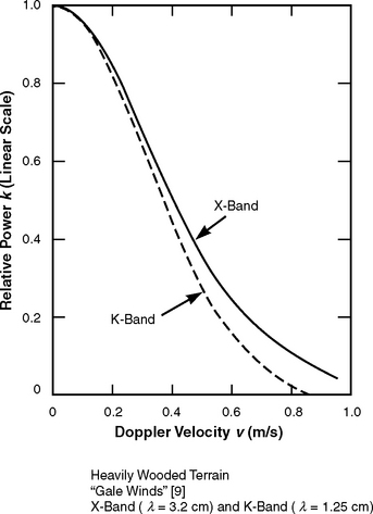
FIGURE 6.57 Measurements of radar ground clutter power spectra by Goldstein under gale winds. (After Goldstein [9]; by permission, The McGraw-Hill Companies, Inc.)
Fresh gale, 39 to 46 mph winds; (9) Strong gale, 47 to 54 mph winds; and (10) Whole gale, 55 to 63 mph winds.
Goldstein’s third measurement was at S-band in “winds of whole gale force.” This spectrum, reported by Goldstein to be of “strange shape” and “markedly out of line with the others” [9], was not shown, although three measured points38 were provided, viz., −1 dB at 0.1 m/s, −3 dB at 0.2 m/s, and −10 dB at 0.7 m/s. However, the autocorrelation function for this measurement was provided by Goldstein and shows a long, slowly diminishing tail plotted on linear scales. Subsequently, Wong, Reed, and Kaprielian [29] computed a corresponding power spectrum as the Fourier transform of a theoretical autocorrelation function incorporating scatterer rotational motion that was a very close match to Goldstein’s unusual experimental autocorrelation function.
Wong, Reed, and Kaprielian’s computed spectrum is reproduced in Figure 6.58 together with the three actual spectral points specified by Goldstein. The computed spectrum shows a long, slowly diminishing tail. Initially, it rapidly drops to power level = 0.2 (–7 dB) at 0.5 m/s, and thereafter slowly diminishes at a rate approximated by a power law of n = 3.3 to power level = 0.02 (–17 dB) at 2 m/s. In comparison, at 2 m/s the widest measured LCE spectrum is at −53 dB. In discussing these curves of correlation function and power spectrum, Wong, Reed, and Kaprielian noted that they “deviate significantly from the usual expected Gaussian shape. Instead, they drop very slowly toward zero” [29]. Thus these data have contributed to the concept of a long spectral tail, here at an usually high power level.

FIGURE 6.58 A radar ground clutter power spectrum computed from Goldstein’s measured correlation function by Wong, Reed, and Kaprielian showing a long spectral tail under winds of whole gale force. (Computed spectrum (solid curve) after [29]; by permission, © 1967 IEEE. Three plotted points from Table 6.8 in Goldstein [9]; by permission, The McGraw-Hill Companies, Inc.)
Some reservations must be accorded to Goldstein’s results, due to their very early origin. Goldstein was attempting to establish only the most basic general characteristics and, indeed, just the very existence of spectral spreading of ground clutter in these early results. Conversion of values from near the limits of Goldstein’s plots on linear scales to decibel quantities for comparison with modern measurements to much lower power levels where the concern is with detailed behavior of spectral tails is using Goldstein’s data out of historical context. In particular, Goldstein’s unusual S-band gale force data and their further elaboration by Wong, Reed, and Kaprielian [29] now appear to be best regarded as an anomalous occurrence in an isolated measurement. No modern measurements of windblown tree clutter spectra under gale force winds are known to exist.
6.6.3.6 ARMAND’S LONG, LOW-LEVEL CLUTTER SPECTRAL TAIL
Armand et al. [14] ostensibly measured X-band clutter spectra from windblown trees to very low levels of spectral power (–120 dB) and correspondingly very high Doppler velocities (20 m/s). Their results are reproduced in Figure 6.59. Armand et al. stated that these ground clutter spectra were measured with CW equipment in which the power received from the sidelobes of the transmitter was an order of magnitude higher than that reflected from the trees. Instabilities were reported to be eliminated through use of klystrons stabilized by cooling with liquid helium. Results were obtained in the 40- to 2,500- Hz Doppler frequency band (i.e., not near the carrier). Spectral results are shown for three wind speeds—4, 13, and 31 mph—over the range from 40 to ∼ 1,300 Hz (0.6 to ∼ 20 m/s). Over this range, the spectral power density levels are between −50 and −120 dB (i.e., are much lower than any other known spectral measurements).
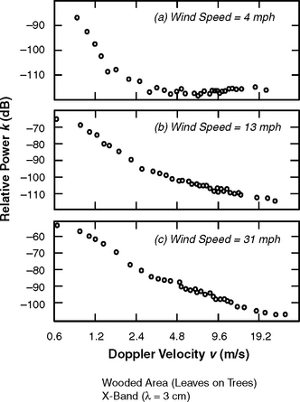
FIGURE 6.59 Measurements of radar ground clutter spectra by Armand et al. of the Russian Academy of Sciences showing very long, low-level spectral tails. After [14], 1975.
For the 4-mph spectrum, the power drops to −120 dB at 2.5 m/s, and thereafter stays at ∼ −120 dB all the way out to 20 m/s (i.e., exhibits a long spectral tail at a uniform low level, like White’s [39] conceptual wideband noise-like spectral component). The 13- and 31-mph spectra drop gradually from −63 and −52 dB, respectively, at 0.6 m/s to ∼ −115 dB at 20 m/s. At power levels 80 dB down, Doppler velocities in the Armand et al. results of Figure 6.59 are ∼ 0.9, 1.4, and 2.5 m/s for 4-, 13-, and 31-mph winds, respectively; these spectral widths are a very close match to those measured by Phase One and LCE at similar levels of spectral power (i.e., near their limits of sensitivity).
Armand et al. [14] claimed that their spectral shapes were power-law, with an average value of power-law exponent n = 3 in the 110- to 2,500-Hz band averaged over all tests and with n varying inversely with wind velocity between 3 and 6 in the 40- to 110-Hz band. The authenticity of these very long, very low-level clutter spectral tails is open to question; what was measured may have been effects of sidelobes, internal system instabilities, etc. Before undue credibility is ascribed to these results, they need to be confirmed by independent and consistent replication using modern measurement instrumentation. However, these results arguably keep open the possibility of long spectral tails at very low power levels below Phase One and LCE sensitivities. As previously discussed, spectral power at large Doppler velocities is theoretically accounted for by Armand et al. through amplitude modulation via leaf rotation and shadowing of one leaf by another, in addition to phase modulation caused by leaf oscillatory motion in the direction of the radar. Note that the Russian spectral measurements [15, 16] that followed those of Armand et al. [14] were performed specifically to obtain information close to the carrier. Although the Phase One and LCE results do not agree with this series of Russian results [13–16] in their assessments of spectral shape as power-law, none of these Russian measurements show inordinately wide spectra over the ranges of spectral power measured by the Phase One and LCE instruments.
6.6.3.7 INSTRUMENTATION AND PROCESSING EFFECTS
Internal effects from the measurement radar often have contaminated and corrupted attempted measurements of clutter frequency spectra to low spectral power levels. The fact that the shape of the spectrum resulting from oscillator instability is an n = 3 power law can raise suspicion of measured clutter spectra with n = 3 power-law characteristics. For example, the Simkins et al. [17] heavily-wooded-valley data of unusually wide spectral extent follow an n = 3 power-law shape, as do the Armand et al. [14] data at very low power levels (70 to 120 dB down) and high Doppler velocities (1.65 to 37.5 m/s). Care must be taken to isolate and avoid spectral contamination from system instabilities.
Quantification of spectral contamination is required for every measurement at the actual range at which the clutter measurement is performed, since instability of the stable local oscillator (STALO) produces a greater effect at longer ranges (the phase has more time to change when the STALO is used to upconvert on transmit and downconvert on receive). If the STALO is not used on receive, but the signal is merely envelope-detected prior to spectral analysis (as in the results of Goldstein [9] and Fishbein et al. [10]), the full STALO instability spectrum or that of the transmitter is impressed on the received clutter signal. Goldstein’s [9] early measurements were undoubtedly made using a klystron or magnetron as the transmitter, resulting in relatively poor stability.
In the Armand et al. [14] results, transitions are observable in the spectral data at low power levels (at 1.5 m/s Doppler velocity for 4-mph wind speed, and at 2.4 m/s Doppler velocity for 13-mph wind speed). For Doppler velocities greater than those of these transition points, it is conceivable that the data result from system instabilities. Note that the results of Armand et al. were obtained using a CW transmitter; use of pulsed radar can introduce additional instability due to noise contamination of trigger pulses. Nonlinearities in circuitry or processing (e.g., lin-limit amplifier) can also limit and spread the frequency spectrum, especially under strong signal (strong clutter) conditions. Data in saturation result in significant spectral spreading caused by the actual spectrum convolving with itself in such circumstances. Discounting this possibility for the stationary false alarm cells underlying the Simkins et al. heavily-wooded-valley data is the reported fact that spectra from adjacent non-false alarm cells of similar intensity were narrower. Unwanted antenna motion caused mechanically, and/or by the wind, can also spread the frequency spectrum by modulating the clutter signal. This modulation may go unobserved if stability testing is performed in low-wind conditions.
A few cases of long spectral tails extending to Doppler velocities >> 3 m/s were observed during the course of examining the Phase One database of spectral measurements. In every case, the long spectral tail was isolated to some sort of instrumentation problem (e.g., sticking bits on the A/D converter generating minute sample-and-hold stairsteps on the temporal signal, occasional saturations, external interference). One excessively wide Phase One spectral measurement caused by undetected saturation was inadvertently included in a set of “windy” spectra in a previous publication (spectrum 4, Figure 6.9, in [21]). Thus any unusually wide measured spectra should always be very carefully examined in the time domain before accepting the wide frequency domain result.
Attempts to improve Phase One stability by sampling the transmitted signal and correcting (i.e., subtracting) transmitted phase variations in the received signal were unsuccessful (i.e., proved to be not simple to implement). The LCE radar was a spectrally purer system than the Phase One radar and was never observed to generate an excessively wide spectral tail due to system or processing contamination. A number of windblown clutter spectral measurements by other investigators reviewed from time to time by the author have at first contained obviously corrupted clutter spectral tails of excessive width and extremely slow (e.g., n ≅ 3) decay; subsequent investigation has always found these long spectral tails to be caused by errors in instrumentation or processing. In considering all the possible ways in which instrumentation limitations or processing errors can broaden measured clutter spectra, it is well to bear in mind that of two measured spectra—one narrow and one wide—ostensibly characterizing the same clutter phenomenon, the narrower spectrum is always more credible since all corruptive influences due to instrumentation limitations or processing errors can only broaden the spectrum, not narrow it.
Because of all the potential uncertainties (i.e., potential contaminants of internal and external origin) in radar ground clutter spectral measurements as exemplified in the preceding discussions of Section 6.6.3, the use of such data requires the exercise of judgment. Ground clutter spectral models should reflect, for the most part, central repeatable trends in measured data, not unusual or isolated artifacts or aberrations.
6.7 SUMMARY
Accurate characterization of radar ground clutter spectral shape is important in radar technology applications in which target signals compete with strong ground clutter returns. Ground clutter spectral spreading can limit the performance of MTI/Doppler processors, including both conventional one-dimensional fixed-parameter designs [1, 2] and modern two-dimensional displaced phase-centered antenna or space-time adaptive techniques [3–5] for detecting and tracking moving targets in clutter backgrounds. Internal clutter motion can also cause defocusing in SAR processing [62] and indeed can degrade any radar processing technique that assumes the clutter to be stationary. Such reasons provide motivation to obtain a proper understanding of clutter spectral spreading and to obtain an accurate characterization of the shapes of clutter spectra to very low levels of spectral power. Historically, the state of knowledge of windblown ground clutter spectral shape has been rather poor, and considerable disagreement has existed concerning the extent to which Doppler spreading occurs in such spectra.
Lincoln Laboratory measurement data indicate that ground clutter power spectra over spectral dynamic ranges reaching 60 to 80 dB below the zero-Doppler peaks are relatively narrow and reasonably characterized as of exponential shape. First observation of exponential spectral decay in the clutter studies discussed herein occurred in the early examination of windblown foliage clutter spectra obtained with the Phase One clutter measurement radar at western Canadian sites. These first observations of exponential decay remained valid in the general representation of a much more complete set of L-band spectral measurements over various regimes of wind speed obtained with the Phase One radar at the Lincoln Laboratory measurement site of Katahdin Hill in eastern Massachusetts [21].
Exponential decay was also concluded to be the best overall characterization of windblown ground clutter spectral shape covering Phase One measurements at other frequencies (i.e., VHF, UHF, S-, and X-bands), from other sites, and over several thousand spectral observations taken from the extensive L-band database of clutter spectral measurements subsequently obtained with the LCE clutter measurement radar [25]. The LCE radar was a major L-band-only upgrade of the five-frequency Phase One radar with new, much improved receiver and data recording units, lower phase noise levels, and very clean and reliable spectral response. Analyses of Phase One clutter data in Canada [22, 23] and in the U. K. [24] also concluded that ground clutter spectra were generally best-fitted with exponential shapes.
On the basis of the Phase One and LCE clutter data, two different first-principles theoretical models [39, 60] were independently developed for the windblown clutter Doppler spectrum that, although mathematically complex, in both cases provide close to exponential decay under numerical evaluation. Other previous references to exponential (or quasi- or partially-exponential) clutter spectral decay exist in a much earlier Lincoln Laboratory measurement program [59] of the 1970s, and in Russian measurements [13–16] and French measurements [38] of the same early time period.
The very earliest indications were that windblown ground clutter spectra were of Gaussian spectral shape [6–9]. Many subsequent measurements to lower power levels 30 to 40 dB below the peak zero-Doppler level indicated spectral shapes that were significantly wider than Gaussian in their tails and that appeared to be well approximated with power-law functions [10–20]. The Phase One and LCE ground clutter spectral measurements, over such limited spectral dynamic ranges, also can be adequately modeled as of power-law shapes. However, the Phase One and LCE measurement data also clearly indicate that the power-law rates of decay at upper levels of spectral power do not continue to lower levels of spectral power reaching 60 to 80 dB down from the zero-Doppler peak. The measured power-law rates of decay at lower power levels are always much faster than at the upper levels.
An exponential representation generally captures, at least approximately and occasionally highly accurately, the major attributes of the windblown clutter ac spectral shape function over the entire range from near the zero-Doppler peak to measured levels 60 to 80 dB down. In contrast, the windblown clutter ac spectral shape is not at all representable by any power law over such a wide spectral dynamic range. The maximum Phase One- and LCE-measured Doppler velocity spectral extents from windblown foliage at levels 60 to 80 dB down are ≈3 to 4 m/s. Power-law models can extrapolate data of 40-dB spectral dynamic range to spectral extent as great as 30 m/s, 60 dB down. Such extreme windblown foliage spectral extents have never been corroborated by any results in the extensive Phase One and LCE databases of windblown clutter spectral measurements.
Chapter 6 provides a new empirical model for windblown ground clutter Doppler spectra based on many clutter spectral measurements obtained with the Lincoln Laboratory LCE and Phase One five-frequency (VHF, UHF, L-, S-, and X-band) radars. This model is complete, including both ac and dc components of the spectrum. The important parameters incorporated in the model are wind speed and radar carrier frequency. Ac spectral shape is specified as exponential, with the Doppler-velocity exponential shape factor strongly dependent on wind speed but independent of radar frequency, VHF to X-band. The fact that ac spectral spreading occurs at VHF in windblown clutter Doppler-velocity spectra more or less equivalently as at X-band is illustrated through representative measurement results; many other examples of VHF-measured clutter spectra with similar spectral spreading exist in the Phase One and LCE databases.
The major difference between VHF and X-band clutter spectra is that a much larger dc spectral component exists at VHF compared with X-band. The ratio of dc to ac spectral power in the model is determined by an analytic expression empirically derived from the measurements that captures the strong dependencies of dc/ac ratio on both wind speed and radar frequency. Chapter 6 includes both a complete specification of the clutter spectral model and a thorough comparison of model predictions with many examples of measured windblown clutter spectra under various combinations of radar parameters and measurement circumstances. Besides wind speed and radar frequency, other parameters that might be thought to significantly influence clutter spectra, but that appear to be largely subsumed within general ranges of statistical variability in the measurement data, include tree species, season of the year, wind direction, cell size, polarization, range, and grazing angle. The exponential model is explicitly derived to be applicable to windblown trees, but examples are also provided of measured clutter spectra from scrub desert, cropland, and rangeland that indicate the model can also perform adequately for other windblown vegetation types by suitably adjusting its dc/ac term.
Although it is now generally accepted that radar ground clutter spectral shapes are wider than Gaussian in their tails, the simple Gaussian continues to be how clutter spectra are usually represented in radar system engineering (at least as a method of first approach in representing effects of intrinsic clutter motion) because of its simplicity and analytic tractability. The Gaussian spectral shape is theoretically generated by a group of moving scatterers, each of random translational drift velocity [19]. Theory also suggests that the origin of the increased spreading observed in measured ground clutter spectra beyond that predicted by Gaussian is largely due to the random oscillatory motion of leaves and branches, in contrast to simple random translational motion [19, 29, 42]. Like the Gaussian spectral shape, the exponential spectral shape is also simple and analytically tractable and has the advantage of being wider than Gaussian as required by experiment and supported by theory.
There is no underlying fundamental physical principle requiring clutter spectra to be precisely of exponential shape. Many of the Phase One and LCE clutter spectral measurements, particularly many of the narrower spectra occurring at lower wind speeds, are less exponential overall than some of the wider measured spectra. To be clear on this matter, almost none of the Phase One- and LCE-measured clutter spectra can be accurately represented by any single simple analytic function, including exponential [31], over their complete spectral dynamic ranges, from the point of view of passing rigorous statistical hypothesis tests. Use of the exponential shape in Chapter 6 is as a convenient analytic bounding envelope that empirically approximates, occasionally very accurately, many of the LCE and Phase One measurements over most of their spectral dynamic ranges, including the lowest power levels measured. The resulting model overcomes much of the difficulty in modeling clutter spectra not only by using exponential shapes, but also by introducing the concept of a quasi-dc region and absorbing the excess power measured in the quasi-dc region into the dc delta function term of the model. This approach allows the model the flexibility of using the exponential representation to optimally match the measured spectral spreading in the spectral tail regions without regard to the narrow near-zero-Doppler quasi-dc region, which often displays a different rate of decay than occurs in the broad spectral tail [31].
In addition to showing that measured shapes of windblown ground clutter Doppler spectra appear to be much more closely matched by an exponential approximation than by Gaussian (too narrow) or power-law (too wide) approximations, Chapter 6 also investigates the impact of assigning the correct clutter spectral shape on MTI and STAP coherent target detection. Compared to the exponential shape, the Gaussian shape substantially underpredicts the effects of clutter on detection, and the power-law shape substantially overpredicts the effects of clutter on detection. The exponential spectral model for windblown foliage is validated by showing that the differences in clutter improvement factor performance prediction between using actual measured I/Q data as input to the clutter canceller, and modeled clutter data of Gaussian, exponential, or power-law spectral shape, are minimized when the spectral model employed is of exponential shape.
It is evident on the basis of the Phase One and LCE measurements that the current state of knowledge regarding the extent of spectral spreading in windblown ground clutter has been advanced to the point where it is relatively incontrovertible that clutter spectra from windblown vegetation, although wider than Gaussian, are still generally relatively narrow and spread to Doppler velocities < ≈ 3 or 4 m/s over spectral power levels reaching to 80 dB below zero-Doppler peaks for wind speeds in the 15- to 30-mph range. Investigators who may wish to continue to argue for much wider clutter spectra from windblown foliage over such ranges are faced with proving spectral purity in their wider measurements, since unknown corruptive instrumentation or processing effects can only widen spectra, not narrow them. Presumably, most of the spectral spreading that occurs in the Phase One and LCE data is caused by the velocity distribution (translational and/or oscillatory) of the foliage, that is, by the radial motion of individual scatterers (leaves and branches) toward and away from the radar causing phase modulation in the returned signal. To whatever extent other effects are also at work in the Phase One and LCE data, such as leaf rotation or the shadowing of one leaf by another causing more complex amplitude modulation effects, such effects are also constrained to cause limited spreading to levels 80 dB down.
Chapter 6 also provides a relatively thorough review of the available literature of clutter spectral measurements, which generally brings it and the Phase One and LCE results into conformity and agreement. There remain hints in the literature, however, not only from theoretical reasoning but also in various poorly substantiated measurement results, of long spectral tails existing in ground clutter data to Doppler velocities greatly exceeding the maximum ≈ 3 to 4 m/s observed in the Phase One and LCE data. Arguments for the existence of such wide tails often are based on postulated leaf-rotation and leaf-shadowing effects. Such long tails have never been observed, whether as slowly decaying power laws or as uniform-amplitude wideband noise-like components, in any of the several thousand spectra that have been examined from the extensive Phase One and LCE databases of ground clutter spectral measurements to levels reaching 60 to 80 dB below zero-Doppler peaks. What might occur at lower levels remains conjectural.
REFERENCES
1. Skolnik, M. I. Introduction to Radar Systems, 3rd ed. New York: McGraw-Hill, 2001.
2. Scheer J. A., Kurtz J. L., eds. Coherent Radar Performance Estimation. Boston, MA: Artech House, Inc., 1993.
3. Klemm, R. Space-Time Adaptive Processing: Principles and Applications. : IEE Press, Radar, Sonar, Navigation and Avionics Series, 1999.
4. Ward, J. “Space-Time Adaptive Processing for Airborne Radar,”. Lexington, MA: MIT Lincoln Laboratory, Technical Rep. 1015, 13 December 1994. [DTIC AD-A293032. ].
5. P. Richardson, “Relationships between DPCA and adaptive space-time processing techniques for clutter suppression,” Proc. International Conf. Radar, SEE 48 rue de la Procession, 75724 Paris Cedex 15 (May 1994), pp. 295–300.
6. Ridenour L. N., ed. Radar System Engineering. in the MIT Radiation Laboratory Series; Vol. 1. McGraw-Hill, New York, 1947. [Reprinted, Dover Publications (1965). ].
7. Barlow, E. J. “Doppler Radar,”. Proc. IRE. 37(4), 1949.
8. Lawson J. L., Uhlenbeck G. E., eds. Threshold Signals. in the MIT Radiation Laboratory Series; Vol. 24. McGraw-Hill, New York, 1950.
9. Goldstein, H. “The Fluctuations of Clutter Echoes,” pp. 550–587. In: Kerr D. E., ed. Propagation of Short Radio Waves, Vol. 13 in the MIT Radiation Laboratory Series. New York: McGraw-Hill, 1951.
10. Fishbein, W., Graveline, S. W., Rittenbach., O. E. “Clutter Attenuation Analysis,” Fort Monmouth, NJ: U. S. Army Electronics Command, Technical Rep. ECOM-2808 (March 1967). In: Schleher D. C., ed. Reprinted in MTI Radar. Boston, MA: Artech House, Inc., 1978.
11. Warden, M. P., Wyndham, B. A. “A Study of Ground Clutter Using a 10-cm Surveillance Radar,”. In: Royal Radar Establishment, Technical Note No. 745. U. K. : Malvern; 1969. [DTIC AD 704874. ].
12. N. C. Currie, F. B. Dyer, and R. D. Hayes, “Radar Land Clutter Measurements at Frequencies of 9. 5, 16, 35, and 95 GHz,” Engineering Experiment Station, Georgia Institute of Technology, Technical Report No. 3, United States Army, Contract DAAA-25-73-C-0256, April 1975. DTIC AD-A012709.
13. Kapitanov, V. A., Mel’nichuk, V., Chernikov, A. A. “Spectra of radar signals reflected from forests at centimeter waves,”. Radio Eng. and Electron. Phys. 18(9), 1973.
14. Armand, N. A., Dyakin, V. A., Kibardina, I. N., Pavel’ev, A. G., Shuba, V. D. “The change in the spectrum of a monochromatic wave when reflected from moving scatterers,”. Radio Eng. and Electron. Phys. 20(7), 1975.
15. Andrianov, V. A., Bondarenko, I. S., Kibardina, I. N., Prosshin, V. K., Shtern, D. Y. “Characteristics of measurement of spectra of radio signals scattered by an underlying surface,”. Radio Eng. and Electron. Phys. 21(2), 1976.
16. Andrianov, V. A., Armand, N. A., Kibardina, I. M. “Scattering of radio waves by an underlying surface covered with vegetation,”. Radio Eng. and Electron. Phys. 21(9), 1976.
17. W. L. Simkins, V. C. Vannicola, and J. P. Ryan, “Seek Igloo Radar Clutter Study,” Rome Air Development Center, Technical Rep. RADC-TR-77-338 (October 1977). Updated in FAA-E-2763b Specification, Appendix A (May 1988). See also FAA-E-2763a (September 1987), FAA-E-2763 (January 1986, July 1985).
18. Jiankang, J., Zhongzhi, Z., Zhong, S. “Backscattering power spectrum for randomly moving vegetation,”. In: Proc. IGARSS Symposium. Zurich: ; August 1986:1129–1132.
19. Li, N. J., “A study of land clutter spectrum,”Suzuki T., Ogura H., Fujimura S., eds. Proc. 1989 International Symp. on Noise and Clutter Rejection in Radars and Imaging Sensors. IEICE,: Kyoto, 1989; 48–53.
20. G. W. Ewell, private communication (December 1995).
21. Billingsley, J. B., Larrabee, J. F. “Measured Spectral Extent of L- and X-Band Radar Reflections from Windblown Trees,”. Lexington, MA: MIT Lincoln Laboratory, 6 February 1987. [Project Rep. CMT-57 DTIC AD-A179942. ].
22. Chan, H. C. “Spectral Characteristics of Low-Angle Radar Ground Clutter,”. Ottawa, Canada: Defence Research Establishment Ottawa, December 1989. [Report No. 1020 DTIC AD-A220817. ].
23. Chan, H. C. “Radar ground clutter measurements and models, part 2: Spectral characteristics and temporal statistics,”. In: AGARD Conf. Proc. Target and Clutter Scattering and Their Effects on Military Radar Performance. Ottawa: ; 1991. AGARD-CP-501 AD-P006374.
24. Sarno, G. C. “A model of coherent radar land backscatter,”. In: AGARD Conf. Proc. Target and Clutter Scattering and Their Effects on Military Radar Performance. Ottawa: ; 1991. [AGARD-CP-501 AD-P006375. ].
25. Billingsley, J. B. “Exponential Decay in Windblown Radar Ground Clutter Doppler Spectra: Multifrequency Measurements and Model,”. Lexington, MA: MIT Lincoln Laboratory, Technical Report 997, 29 July 1996. [DTIC AD-A312399. ].
26. J. B. Billingsley, “Windblown radar ground clutter Doppler spectra: measurements and model,” submitted to IEEE Trans. AES, May 2000, accepted subject to minor revision, October 2000.
27. Long, M. W. Radar Reflectivity of Land and Sea, 3rd ed. Boston: Artech House, Inc., 2001.
28. Nathanson, F. E. Radar Design Principles, 2nd ed. New York: McGraw-Hill, 1991. [Reprinted, SciTech Publishing, Inc., 1999. ].
29. Wong, J. L., Reed, I. S., Kaprielian, Z. A. “A model for the radar echo from a random collection of rotating dipole scatterers,”. IEEE Trans. AES. 3(2), 1967.
30. Greco, M. V., Gini, F., Farina, A., Billingsley, J. B. “Analysis of clutter cancellation in the presence of measured L-band radar ground clutter data,”. In: Proceedings of IEEE International Radar Conference (Radar 2000). Alexandria, VA: ; May 8–12, 2000.
31. Greco, M. V., Gini, F., Farina, A., Billingsley, J. B. “Validation of windblown radar ground clutter spectral shape,”. IEEE Trans. AES. Vol. 37(no. 2), April 2001.
32. Billingsley, J. B., Farina, A., Gini, F., Greco, M. V., Lombardo, P. “Impact of experimentally measured Doppler spectrum of ground clutter on MTI and STAP,”. In: Proceedings of IEE International Radar Conference (Radar ‘97), IEE Conf. Pub. No. 449, pp. 290-294. Edinburgh: ; October 1997:14–16.
33. Lombardo, P., Greco, M. V., Gini, F., Farina, A., Billingsley, J. B. “Impact of clutter spectra on radar performance prediction,”. IEEE Trans. AES. Vol. 37(no. 3), July 2001.
34. Billingsley, J. B., Larrabee, J. F. “Bragg Resonance in Measured L-band Radar Clutter Doppler Spectra from Inland Water,”. Lexington, MA: MIT Lincoln Laboratory, Technical Rep. 1019, 1 August 1995. [DTIC AD-A297680. ].
35. Billingsley, J. B. “Measurements of L-band inland-water surface-clutter Doppler spectra,”. IEEE Trans AES. April 1998; Vol. 34(No. 2):378–390.
36. Ferranti, R. L. “Very low phase noise in a pulsed 10-kw L-band triode power amplifier,”. In: Proc. RF Expo West. Santa Clara, CA: ; February 1991:59–66.
37. Harris, F. J. “On the use of windows for harmonic analysis with the discrete Fourier transform,”. Proc. IEEE. January 1978; 66:51–83.
38. Basard, R. “Vegetation clutter Doppler spectrum models,”. In: International Conference on Radar, (Session II). Paris: ; December 1978:28–31. 4–8
39. White, R. G. “A model for MTI radar clutter,”. In: Proc. SEE Int. Radar Conf. Paris: ; May 1994:540–545.
40. Narayanan, R. M., Doerr, D. W., Rundquist, D. C. “Temporal decorrelation of X-band backscatter from wind-influenced vegetation,”. IEEE Trans. Aerosp. Electron. Syst. 1992; 28(2):404–412.
41. Narayanan, R. M., Nelson, S. E., Dalton, J. P. “Azimuthal scattering pattern of trees at X-band,”. IEEE Trans. Aerosp. Electron. Syst. 1993; 29(2):588–593.
42. Narayanan, R. M., Doerr, D. W., Rundquist, D. C. “Power spectrum of wind-influenced vegetation backscatter at X-band,”. IEE Proc. -Radar, Sonar Navig. 1994; 141(2):125–131.
43. Stewart, N. A. “Use of crosspolar returns to enhance target detectability,”. In: Clarke J., ed. Advances in Radar Techniques, IEE Electromagnetic Wave Series 20. London, U. K. : Peter Peregrinus, Ltd. ; 1985:449–454.
44. Billingsley, J. B., Larrabee, J. F. “Multifrequency Measurements of Radar Ground Clutter at 42 Sites,”; Volumes 1, 2, 3. MIT Lincoln Laboratory, Technical Rep. 916, Lexington, MA, 15 November 1991. [DTIC AD-A246710. ].
45. de Loor, G. P., Jurriens, A. A., Gravesteijn, H. “The radar backscatter from selected agricultural crops,”. IEEE Trans. on Geoscience Electronics. April 1974; 12:70–77.
46. Kelly, E. J. “An adaptive detection algorithm,”. IEEE Trans. on Aerospace and Electronic Systems. March 1986; Vol. 22(No. 2):115–127.
47. Farina, A., Lombardo, P., Pirri, M. “Non-linear space-time processing for airborne early warning radar,”. IEE Proc. on Radar, Sonar and Navigation. February 1998; Vol. 145(No. 1):9–18.
48. Klemm, R. “Adaptive clutter suppression for airborne phased-array radars,”. IEE Proceedings-F. February 1983; Vol. 130(No. 1):125–132.
49. Barbarossa, S., Farina, A. “Space-time-frequency processing of synthetic aperture radar signals,”. IEEE Trans. on Aerospace and Electronic Systems. April 1994; Vol. 30(No. 2):341–358.
50. Barton, D. K. Modern Radar System Analysis. Artech House, Inc., Boston, MA, 1988:246.
51. Papoulis, A. The Fourier Integral and Its Applications. New York: McGraw-Hill, 1962.
52. Davenport, W. B., Jr., Root, W. L. An Introduction to the Theory of Random Signals and Noise. New York: McGraw-Hill, 1958.
53. Goldman, S. Frequency Analysis, Modulation, and Noise. New York: McGraw-Hill, 1948. [Reprinted, Dover Publications (1967). ].
54. Bass, F. G., Bliokh, P. V., Fuks, I. M. “Statistical characteristics of a signal scattered from randomly moving reradiators on a plane section,” translated from. Radiotechnika i Electronika (USSR). May 1965; 10(5):731–739.
55. Rosenbaum, S., Bowles, L. W. “Clutter return from vegetated areas,”. IEEE Trans. Ant. Propag. March 1974; AP-22(2):227–236.
56. Schleher, D. C. MTI and Pulsed Doppler Radar. Artech House, Norwood, MA, 1991:127.
57. Scheer, J. A. “Coherent Radar Performance Estimation,”. In: IEEE National Radar Conference, Tutorial Notes. Atlanta: ; 1994.
58. Currie N. C., Brown C. E., eds. Principles and Applications of Millimeter-Wave Radar. Norwood, MA: Artech House, Inc., 1987.
59. Cartledge, L., Labitt, M., Teele, J. H., Yates, R. D. “An Experimental UHF Ground Surveillance Radar, Volume 2,”. Lexington, MA: MIT Lincoln Laboratory, Technical Rep. 497, 12 October 1972. [DTIC AD-757565. ].
60. Lombardo, P., Billingsley, J. B. “A new model for the Doppler spectrum of windblown radar ground clutter,”. In: Proceedings of 1999 IEEE Radar Conference. Boston, MA: ; April 1999:20–22. [pp. 142–147. ].
61. R. G. White, private communication (11 September 1995).
62. Elachi, C., Evans, D. D. “Effects of random phase changes on the formation of synthetic aperture radar imagery,”. IEEE Trans. on Antennas and Propagation. January 1977; Vol. AP-25(No. 1):149–153.
32.The term “Doppler velocity” as used herein is equivalent to scatterer radial velocity.
33.In Chapter 6, r represents dc/ac ratio. In preceding chapters, r represents radar range (see Section 2.3.1.1).
34.In Chapter 6, f represents Doppler frequency and fo represents radar carrier frequency. In preceding chapters, f represents radar carrier frequency.
35.Formed from all 16 primary-swath gates at Beulah, not just the six pure-wheat gates for which results are shown in Figure 6.25.
36.The summary provided here includes material originally published in [30, 31, and 33] by permission of IEEE, and in [32] by permission of IEE.
37.The Beaufort scale of wind velocities covers 13 Beaufort force numbers [from (0) Calm and (1) Light air to (12) Hurricane], including the following “gale force” numbers: (7) Moderate gale, winds from 32 to 38 mph; (8)
38.Labelled as occurring at wind speed of 50 mph in Goldstein’s Table 6.8 [9].