
PRELIMINARY X-BAND CLUTTER MEASUREMENTS
2.1 INTRODUCTION
Chapter 2 provides general information describing the amplitude distributions of X-band land clutter returns received from regions of visible ground, based on Phase Zero measurements at 106 sites. Subsequent chapters provide similar information at other frequencies. In presenting land clutter data and results, Chapter 2 attempts both to do justice to describing a very complex phenomenon, and also to efficiently provide useful and easily accessible modeling information. The result is a chapter that provides increasing insight into the clutter phenomenon by cyclically building up an understanding of the many interacting influences affecting clutter amplitude statistics. As insights are developed, they are accompanied with the presentation of modeling information that generalizes such influences at various levels of fidelity.
2.1.1 OUTLINE
The major results of Chapter 2 are summarized within this section.
Basic Clutter Modeling Information. Chapter 2 provides basic ensemble modeling information describing X-band clutter amplitude distributions over macropatches of visible terrain as a function of depression angle for three comprehensive terrain types—rural/low-relief, rural/high-relief, and urban. Chapter 2 goes on to explain, enlarge upon, and extend the nature of low-angle clutter amplitude statistics as encoded within the basic modeling information.
Angle Characteristic. There traditionally has existed within the body of ground clutter literature the idea that a clutter model could be a simple characteristic of clutter strength vs illumination angle. Such a model is provided in Chapter 2 as an expected-value generalization of all the Phase Zero measurements. However, ground clutter is inherently a statistical phenomenon in which large statistical variation occurs. Thus this simple angle-characteristic model shows two characteristics of clutter strength, mean and median, vs angle. Together these characteristics demonstrate the important fact that clutter is statistical and show not only clutter strength vs angle, but also specify the variability (i.e., mean-to-median ratio) of clutter strength at any given angle.
Worst-Case Situations. The basic X-band modeling information of Chapter 2 provides general information. Chapter 2 also provides upper bounds on how strong ground clutter can become in exceptional circumstances by comparing the amplitude distributions from the strongest Phase Zero clutter patches (urban clutter, mountain clutter) with those of the basic information.
Fine-Scaled Variations with Terrain. The basic modeling information separates terrain into just three categories, which, simply interpreted, implies that, in general, only “mountains” (rural/high-relief terrain) and “cities” (urban terrain) warrant separation from all other terrain types (rural/low-relief terrain). However, with decreasing significance finer trends occur in the Phase Zero data with more specific description of terrain type. Within rural low-relief terrain, fine-scaled differences in clutter amplitude statistics among wetland, forest, and agricultural land are shown to exist. Within urban terrain, fine-scaled differences between terrain of residential (i.e., low-rise) and commercial (i.e., high-rise) character are illustrated. The effect of trees as discrete scattering sources is discussed. Modeling information in which, on low-relief open terrain, trees are the predominant X-band discrete scattering source, and such that clutter amplitude distributions vary with the relative incidence of occurrence of trees (i.e., percent tree cover), is provided.
Negative Depression Angle. Negative depression angles occur when terrain is observed by the radar at elevations above the antenna. Such terrain is usually rough and steep. Information is provided describing clutter amplitude distributions occurring at negative depression angles.
Non-Angle-Specific Modeling Information. Chapter 2 principally provides generalized X-band modeling information for clutter amplitude statistics as a function of depression angle. However, the chapter also provides some non-angle-specific modeling information. For example, the overall distribution that results from combining all of the Phase Zero measured clutter samples is specified, irrespective of terrain type and depression angle, into one all-encompassing ensemble distribution. Much information concerning frequency of occurrence of various levels of low-angle clutter strength is contained in this overall distribution, as measured from 2,177 clutter macropatches at 96 different sites. Chapter 2 also provides non-angle-specific expected value information by showing distributions of mean patch clutter strength by landform and land cover, respectively. To the extent that the overall terrain at a given radar site may be classified as being of one terrain class, such information can characterize mean clutter strength over the whole site, not only in terms of most likely values, but also in terms of worst-case (strong clutter) and best-case (weak clutter) values.
Appendices. The appendices of Chapter 2 provide discussions of the following subjects: (a) Phase Zero measurement equipment and calibration, (b) formulation of clutter statistics, and (c) numerical computation of depression angle.
2.2 PHASE ZERO CLUTTER MEASUREMENTS
2.2.1 RADAR INSTRUMENTATION
The pilot phase clutter measurements and modeling program was designated as Phase Zero. The Phase Zero radar was a pulsed system (0.5 μs pulse width for many of the Chapter 2 results) that operated at X-band (9375 MHz) with horizontal polarization. The primary display of this radar was a 16-inch diameter, digitally generated, PPI unit. A precision IF attenuator was installed in the radar receiver as a means of measuring clutter strength. The radar was put under control of a minicomputer, by means of which a raw digital record of clutter strength could be obtained by digitally recording the contents of the PPI display in stepped levels of attenuation (1-dB steps over a 50-dB dynamic range).
For many of the results of Chapter 2, the maximum PPI range was set at 12 km, and the clutter data sampling interval size in the polar PPI display was 37 m in range extent and ∼0.25° in azimuth extent.
The radar and digital recording equipment were installed in an all-wheel drive one-ton truck that was equipped with a 50-ft pneumatically extendable antenna mast and self-contained prime power. With this mobile Phase Zero clutter measurement instrument, clutter data were recorded in surveillance mode from all clutter sources within the field-of-view by azimuthally scanning the beam which was narrow (0.9°) in azimuth, wide (23°) in elevation, and fixed horizontally at zero degrees depression angle, through 360° in azimuth. Azimuthally scanned data were acquired at each site for each of seven experiments of increasing maximum range from 1.5 to 94 km. Clutter strength calibration was based on the elevation beam gain applicable at the depression angle at which each clutter patch was measured, not just the boresight gain, even though most patches were measured within the 3-dB elevation beamwidth. Each Phase Zero clutter measurement included internal calibration based on accurate measurement of the minimum detectable signal of the receiver. Occasional external calibrations were performed using balloon-borne spheres as test targets. The Phase Zero radar is more fully described in Appendix 2.A.
2.2.2 MEASUREMENT SITES
Figure 2.1 shows the location of all 106 sites at which Phase Zero ground clutter measurements were obtained. Photographs of the terrain at two of the measurement sites are shown in Figure 2.2. Figure 2.2(a) shows low-relief undulating prairie farmland at the Beiseker site located 75 km northeast of Calgary. Figure 2.2(b) shows high-relief mountainous terrain at the Plateau Mountain site located 120 km southwest of Calgary in the Canadian Rocky Mountains. Significantly different backscatter characteristics would be expected, and indeed were measured, from the terrain in Figure 2.2(a) compared with that of Figure 2.2(b). However, later in Chapter 2 it will be shown that a useful first step in clutter prediction is to simply distinguish terrain type by whether it is of low relief, as pictured in Figure 2.2(a), or of high relief, as pictured in Figure 2.2(b).
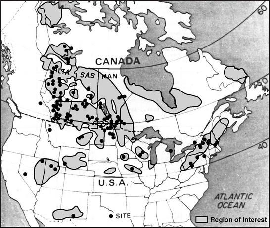

FIGURE 2.2 Two clutter measurement sites in Alberta, Canada. (a) Low-relief farmland at Beiseker. (b) High-relief mountainous terrain at Plateau Mt.
The Phase Zero radar served in a pilot role in site selection activities for Phase One measurements. It is apparent in Figure 2.1 that many of the measurement sites were in Canada. The Phase Zero and Phase One clutter measurement programs were jointly conducted by the United States and Canada within an intergovernmental Memorandum of Understanding. Coordinated analyses of the measurement data took place in both countries [1, 2].
2.2.3 TERRAIN DESCRIPTION
Procedures were developed to systematically describe and classify the clutter-producing terrain at each measurement site. It was necessary that these procedures cause the clutter data, as measured from many sites, to usefully cluster within the same terrain class, and separate between different terrain classes. The terrain within each clutter patch at each site was classified both in terms of the characteristics of its land cover [3] and of its landform or surface relief [4]. The land cover and landform categories utilized in this classification are shown in Tables 2.1 and 2.2, respectively. The classification was performed principally through use of topographic maps and stereo aerial photos, usually at 1:50,000 scale. Since clutter producing terrain is often heterogeneous in its character, even within spatial macropatches, terrain classification often proceeded at two or even three levels to adequately capture the terrain characteristics important in the clutter data.
TABLE 2.1
| 1 | Urban or Built-up Land |
| 11 Residential | |
| 12 Commercial | |
| 2 | Agricultural Land |
| 21 Cropland | |
| 22 Pasture | |
| 3 | Rangeland |
| 31 Herbaceous | |
| 32 Shrub | |
| 33 Mixed | |
| 4 | Forest |
| 41 Deciduous | |
| 42 Coniferous | |
| 43 Mixed | |
| 5 | Water |
| 51 Rivers, Streams, Canals | |
| 52 Lakes, Ponds, Sloughs | |
| 6 | Wetland |
| 61 Forested | |
| 62 Non-Forested | |
| 7 | Barren Land |
TABLE 2.2
Landform Classes and Descriptions
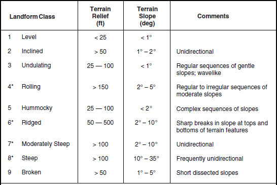
*Classes so indicated are “high-relief;” classes not so indicated are “low-relief.”
In addition to land cover and landform, the height of each site is also important in its effect on the ground clutter measured at that site. High sites see clutter to greater ranges and result in higher depression angles and stronger clutter, compared to low sites. Effective site height is the difference between the terrain elevation of the radar position and the mean of the elevations of all the discernible clutter cells (most of the visible terrain) that occurred at that site. Effective radar height is equal to effective site height plus antenna mast height. By such definition, effective site height and effective radar height are with respect to illuminated terrain only and indicate how high the site or antenna is above the terrain causing clutter backscatter; they are not influenced by masked or shadowed terrain.
The question may be asked as to whether the Phase Zero set of site heights is extensive enough to cover the sorts of height variations that occur in actual radar siting. Figure 2.3 compares site heights for a set of 93 actual radar sites [in Figure 2.3(a)] with Phase Zero site heights [in Figure 2.3(b)], the latter over a set of 93 Phase Zero sites for which effective site height was quantized. In Figure 2.3(a), the 93 actual radar sites were known locations occurring worldwide—of these, 27 occurred around relatively low-relief urban areas, 43 were hilltop sites, and 27 were other sites geographically dispersed (see Appendix 4.B for the definition of “site advantage”). It is seen in Figure 2.3 that this set of other sites provides significantly less extreme siting situations than do the Phase Zero sites. The median Phase Zero site height is 20 m, compared to 10 m for the actual site set. The Phase Zero site set not only encompasses the regime of actual site heights but extends to significantly higher and lower sites. This broad expanse of Phase Zero site heights indicates that the database of clutter measurements that results is not constrained in any unrealistic way—for example, in terms of the range of depression angles available, or the range extents at which clutter occurs, or any other important height-dependent parameter that might affect the clutter results.

2.3 THE NATURE OF LOW-ANGLE CLUTTER
2.3.1 CLUTTER PHYSICS I
2.3.1.1 CLUTTER COEFFICIENT σ°
Radar land clutter is characterized herein in terms of the intrinsic clutter backscattering coefficient σ°, defined to be the radar cross section (RCS) per unit of intercepted surface area A within the spatial resolution cell of the radar on the ground. As shown in Figure 2.4, at the relatively low depression angles α of ground-based radar, the range dimension of A is given by Δr = (c τ/2) sec α, where c is the velocity of propagation (c ≅ 3 × 10⁸ m/s in free space) and τ is the pulse length. The factor of 1/2 in this expression for Δr is necessitated by the two-way round trip travel of the radar pulse. See Section 2.3.4 and Appendix 2.C for definition of depression angle α. The cross-range dimension of A [see Figure 2.4(b)] is given by r·Δθ, where r is slant range to the cell and Δθ, is the one-way 3-dB azimuth beamwidth of the radar. Thus, A is given by A = r·Δθr·Δθ; and σ° is given by σ° = σc/A, where σc is the RCS of the clutter cell under consideration. Appendix 2.A and Appendix 3.C, Eqs. (3.C.1) and (3.C.2), specify how σc is computed in the measurement data.

FIGURE 2.4 Geometry of land clutter for surface radar showing the area A within the radar spatial resolution cell on the ground. (a) Elevation view—range extent Δr is determined primarily by radar pulse length τ. (b) Plan view—cross-range extent is rΔθ, where r is range and Δθ is azimuth beamwidth.
Formulas for A at higher angles where the elevation beamwidth starts to take effect instead of the radar pulse length are available elsewhere (e.g., see [5]). In the ground-based radar results of this book for which α is generally < 2° and at most < ∼8°, not only is A given by A = r·Δr·Δθ, but in addition the sec α factor in Δr differs insignificantly from unity.
In characterizing A some authors have specified Δθ to be the two-way 3-dB azimuth beamwidth rather than the one-way beamwidth (e.g., [6]; see discussion in [7]). The specification of which point on a tapered beam to take as its width in this matter is somewhat arbitrary. The σ° results of this book are based on the more traditional approach of specifying Δθ as the one-way 3-dB beamwidth. If the σ° results of this book had been based on the two-way 3-dB beamwidth, they would have been ∼1 to 2 dB stronger depending upon the actual beam shapes involved.
This book uses the prefix micro to refer to resolution-cell-sized areas on the ground, as shown in Figure 2.4, where Δr in the measured data ranges from 9 to 150 m and Δθ is usually from one to several degrees. Each resolution cell area A contributes a value of σ° into a histogram collected over a much larger region called a clutter patch (see Figure 2.5) consisting of many resolution cells. The prefix macro refers to such large clutter patches. Thus a clutter patch is a spatial macroregion typically several kilometers on a side, usually containing hundreds or thousands of resolution cells.

2.3.1.2 MAJOR ELEMENTS
The major elements that are involved in low-angle clutter are shown in Figure 2.5. Attention is focused on directly illuminated clutter from large kilometer-sized spatial macroregions or patches of visible terrain. Within such clutter patches, at the low angles of ground-based radars, the dominant clutter sources tend to be all of the vertical features on the landscape, either objects associated with the land cover such as trees or buildings, or just the high points of the terrain itself. Such sources are usually spatially localized or discrete in nature, with regions of microshadow occurring between them where the receiver is at its noise floor. As the angle of illumination increases, the amount of microshadowing decreases. As a result, mean strengths in clutter amplitude distributions increase, and spreads (i.e., statistical dispersions) in clutter amplitude distributions decrease with increasing angle. These effects with angle constitute a highly significant parametric dependency in low-angle clutter data, and are emphasized in the modeling information presented in Chapter 2 and throughout the book.
The terrain between the radar and the clutter patch influences the illumination of the clutter patch. For example, multipath reflections can interfere with the direct illumination and cause lobing on the free-space antenna pattern. All such propagation effects (including multipath reflection from intervening low-relief open surfaces; diffraction into shadowed regions over intervening high-relief terrain features; and non-standard refraction through the atmosphere) are included within the pattern propagation factor F, which is defined to be the ratio of the incident field that actually exists at the clutter cell being measured to the incident field that would exist there if the clutter cell existed by itself in free space and on the axis of the antenna beam (see Section 1.5.4). What is measured as clutter strength is the product of the clutter coefficient σ° and the fourth power of the propagation factor. The propagation factor F is a ratio of field strengths (voltages); it appears to the fourth power in clutter strength σ°F4, first because it is squared in going from voltage to power (σ° is a power-like quantity), and second because F2 is squared again to account for the two-way round trip travel of the radar pulse. Clutter strength σ°F4 is the quantity in the radar range equation that requires characterization in dealing with clutter (and propagation to clutter) phenomenology.
At X-band, terrain reflection coefficients are often lower, and hence multipath effects are diminished, from those that can exist at lower radar carrier frequencies. When they exist at X-band, propagation lobes are usually relatively narrow such that typical clutter sources such as trees and buildings over most visible terrain often subtend a number of lobes (see Figure 2.5). As a result, the effects of propagation are diminished and tend to average out at X-band, compared with lower radar frequencies (e.g., VHF) where they can dominate. Throughout this book, clutter strength is given by σ°F4, in units of m2/m2, and is usually expressed in decibels as 10 log10(σ°F4). See Appendix 3.B for further discussion of propagation effects in ground clutter.
2.3.2 MEASURED LAND CLUTTER MAPS
Low Range Resolution (150 m). Figure 2.6 shows Phase Zero X-band measurements of ground clutter in PPI format at six Canadian sites. In each case, the range resolution is 150 m, and the maximum range is 47 km. These data are shown at full Phase Zero sensitivity; cells with discernible clutter return from the ground are shown as white, and cells where the receiver is at its noise floor are shown as black. The terrain at Altona, Manitoba is level cropland. Clutter is measured there only from discrete vertical objects (such as barns, silos, telephone poles, isolated trees, etc.) to a spherical earth horizon (nominally given by 16 km for the 50-ft Phase Zero antenna mast) except for the terrain feature (Pembina Hills) that rises to the far southwest. Only on such level sites is a smooth spherical earth model of terrain applicable in characterizing low-angle microwave clutter. At such level sites, dominant clutter sources are often high cultural or natural discrete objects distributed over the spherical surface.

FIGURE 2.6 Ground clutter maps at six sites. Phase Zero X-band data, 150-m range resolution, horizontal polarization. In each map, maximum range = 47 km, north is zenith, clutter is white, clutter threshold is 8 dB from full sensitivity. PPI scope photos.
At most other sites, even relatively low-relief sites, specific terrain features dominate in low-angle clutter measurements over what would be measured on a spherical earth. Thus, in moving across Saskatchewan (Dana) and into Alberta (Penhold and Beiseker), the terrain becomes more undulating and rolling, and the influence of specific large-scale terrain features dominates over spherical earth effects in the clutter maps for these sites. For example, even in the relatively low-relief terrain at Beiseker, it is the terrain surfaces inclined toward the radar (e.g., to the north and south) from which clutter is received; these surfaces are shadowed (i.e., black) on their far sides. Moving on in Figure 2.6, Burnstick is a forested site in the foothills of the Rocky Mountains, and Plateau Mountain is a site high in the Rockies. To the west at Plateau Mountain, clutter is measured from barren rock faces of high mountain peaks, and to the east clutter is measured looking down at the prairie. Figure 2.2 shows photographs of the terrain at Beiseker and Plateau Mountain.
In all cases in Figure 2.6, the patterns of spatial occurrence of clutter are patchy and granular. The nature of the clutter is on-again, off-again as it arises from discrete sources distributed over surfaces within line-of-sight visibility. The details of each pattern are specific to the terrain features at that site. Digitized terrain elevation data (DTED) are useful for geometrically predicting and modeling the specific nature of the spatial patterns of occurrence of clutter such as are shown in Figure 2.6. Two general observations may be made about all such patterns. First, the amount of clutter that occurs gradually diminishes with increasing range from the site. Second, where clutter occurs (i.e., white patches), its strength is relatively independent of range. Subsequently, Chapter 4 bases the development of non-site-specific modeling information on these two observations. Here attention is focused on the following question: Where clutter occurs (i.e., over spatial regions largely within geometric line-of-sight visibility in which a relatively high percentage of resolution cells contain discernible clutter), what are its spatial amplitude statistics?
High Range Resolution (9 m). Figure 2.7 shows measurements at six sites similar to those of Figure 2.6, but at higher range resolution, namely, 9 m. At this increased resolution (and shorter maximum range, 6 km), the discrete or localized nature of the clutter sources within regions of general terrain visibility is evident. The pattern of vertical cultural objects on the level cropland at Altona is obvious. On the undulating terrain at Beiseker, terrain features are evident in the clutter map, but a rectangular pattern of cultural discretes overlays them. At ranges within 6 km, Dundurn is a military wasteland area of shrub and brush-covered sand dunes, typically 20 to 30 ft high, but without a road grid or cultural overlay. The clutter pattern there is seen to be of granular texture, where the top of each sand dune gives rise to a discrete or localized clutter return. In totality, the high-resolution plots of Figure 2.7 amply illustrate that within directly illuminated clutter regions, the low-angle clutter sources are all of the discrete vertical objects that rise above the surface. These discrete sources are densely distributed within illuminated regions. Clutter returns from the area-extensive terrain surfaces themselves, as opposed to discrete objects rising above these surfaces, are much weaker and, in fact, are often below the sensitivity of the receiver. In viewing the clutter maps of Figure 2.7, a sea of discretes is envisaged as the appropriate physical model for low-angle ground clutter, in contrast to the historical tendency in clutter modeling to associate the phenomenon primarily with area-extensive σ° backscatter from the terrain surfaces themselves (with a relatively few strong discretes such as water towers sometimes added in subsequently as an RCS adjunct; see the preceding discussions of two-component clutter models in Sections 1.2.4 and 1.4.4). The discrete clutter sources that high resolution reveals in Figure 2.7 are also the dominant clutter sources at lower resolution.

FIGURE 2.7 High resolution ground clutter maps at six sites. Phase Zero X-band data, 9-m range resolution, horizontal polarization. In each map, maximum range is 5.9 km, north is zenith, clutter is white, and clutter threshold is reduced by 6 dB to 18 dB from full sensitivity to show strong clutter cells. PPI scope photos.
2.3.3 CLUTTER PATCHES
The approach taken to modeling clutter amplitude statistics in this book is as follows. Within the clutter map measured at each site, clutter patches were selected as spatial macroregions generally within line-of-sight illumination in which a relatively high percentage of resolution cells contained discernible clutter. The meaning of “relatively high” depends on the terrain type and corresponding nature of microshadow in the clutter map. Typically, relatively high meant about 50%, but for high sites and/or steep terrain in which relatively full illumination existed it could approach 100%, and in level terrain in which only isolated discretes were illuminated it could be as low as ∼25%. Overlaying and registering clutter maps onto stereo aerial photographs and topographic maps ensured in patch specification that the terrain within each patch was, in large measure, uniform. Interpretation of the air photos and topographic maps provided descriptive information of the terrain within the patch. For each clutter patch, the distribution of clutter strengths occurring within the patch was obtained and stored in a computer file together with the applicable terrain descriptors of the patch. Altogether, 2,177 clutter patches were selected from the Phase Zero 12-km maximum range experiment at 96 different sites. The modeling task then became one of establishing general correlative properties between the 2,177 stored distributions of measured clutter strength and the corresponding terrain descriptions.
2.3.3.1 CLUTTER PATCHES AT GULL LAKE WEST
Some typical clutter patches and measured clutter patch spatial amplitude distribution from the Gull Lake West site in Manitoba are now shown. Figure 2.8(a) shows a measured clutter map of 12-km radius for Gull Lake West; selected clutter patches within the region are shown in Figure 2.8(b). Figure 2.9 shows the measured amplitude distributions for six of the Gull Lake West patches shown in Figure 2.8.


FIGURE 2.9 Phase Zero clutter statistics and terrain classification for selected patches at Gull Lake West site, February visit.
The terrain from which clutter was measured at Gull Lake West lies in the valley of the Red River and as a result is extremely level. The site itself at Gull Lake West lies on the western brow of a north-south situated ridge about 100 ft above the level terrain to the west, which the site overlooks. The effect of the ridge is to extend the Phase Zero mast height from its nominal 50-ft value to a higher elevation of about 150 ft. Otherwise, the very level terrain at Gull Lake West in some respects represents a canonical situation in which complicating effects of terrain relief are absent. The specific effects observed in the clutter distributions at Gull Lake West are largely caused by variation and complexity in land cover.
Consideration of these effects provides a deeper understanding of the general low-angle clutter amplitude distributions presented subsequently.
Patches 19/1 and 19/2. First consider patches 19/1 and 19/2. These patches are level forested wetland, relatively uncomplicated by the presence of roads, clearings, cultural discretes, and shadowing caused by variations in terrain elevation. Many of the taller trees making up this forested wetland are larch or tamarack. The other major component of the forested wetland is spruce. Also present is an understory of willow. The radar overlooks these patches from its nearby ridge location at a depression angle of ∼1°.
At first consideration, 1° may not seem to be a very large illumination angle, but it is large enough to make all the difference in causing these patches to be fully illuminated obliquely from above, rather than from the side at grazing incidence as they would have been if the radar position had not had its 100-ft terrain elevation advantage. As a result, the clutter histograms for patches 19/1 and 19/2 in Figure 2.9 are uncontaminated by cells at radar noise level (σ°F4 bins containing one or more cells at radar noise level are doubly underlined; these bins appear to the left side of the histograms for the other four patches in Figure 2.9, and indicate the sensitivity limit of the radar in these histograms). That is, every cell in patches 19/1 and 19/2 provides a discernible clutter return, which is not the case for most low-angle clutter patches. In addition, patches 19/1 and 19/2 provide well-behaved histograms of traditional bell shape. In fact, and as expected for full illumination of relatively homogeneous tree foliage, the amplitude distributions for patches 19/1 and 19/2 are very nearly Rayleigh, as is evident from their close match to the Rayleigh slope in the Weibull cumulative plot in Figure 2.9, as well as from the relative values of σ°F4 moments and percentiles listed (in a Rayleigh distribution, mean = standard deviation, skewness = 3 dB, kurtosis = 9.5 dB, mean/median = 1.6 dB, 90 percentile/median = 5.2 dB, 99 percentile/median = 8.2 dB). Note the following matter of terminology—in this book, the adjective “Rayleigh” is often used to specify the situation in which ![]() σ° is Rayleigh-distributed and thus σ° is exponentially distributed (hence the values of moments and percentile ratios just specified apply to the σ° distribution for which
σ° is Rayleigh-distributed and thus σ° is exponentially distributed (hence the values of moments and percentile ratios just specified apply to the σ° distribution for which ![]() is Rayleigh).
is Rayleigh).
Other Patches. Few low-angle clutter patches provide such well-behaved, nearly Rayleigh statistics as do patches 19/1 and 19/2. Over large extents of composite landscape such as typically produce low-angle clutter in surface radars, most sites provide very little in the way of homogeneous terrain. For example, consider patch 18 at Gull Lake West. Although the terrain is level, the land cover is mixed between forest and cropland. At a depression angle of ∼0.5°, the clutter return from the agricultural field surfaces is either masked by the surrounding trees or is below sensitivity at this low angle. As a result, a considerable number of samples in the distribution are at noise level (spike at left side of histogram). To the right of the noise samples, the histogram is less bell-shaped and more spread out than those of patches 19/1 and 19/2 (dotted vertical lines indicating 50, 90, and 99 percentiles are more separated). The cumulative distribution for patch 18 plotted on the Weibull scale in Figure 2.9 is of much lower slope than Rayleigh.
Patches 23 and 26 are relatively similar to patch 18. These three patch distributions as a set (bottom graph, Figure 2.9) characterize much of the clutter-producing terrain at Gull Lake West. Note that these cumulative distributions are shown only above (i.e., to the right of) their regions of noise contamination. Thus, over the regions shown in Figure 2.9, these distributions are not affected by the sensitivity limit of the radar and are what would be measured there by an infinitely sensitive radar. Even on canonically level terrain with an artificially high antenna mast, complexity and heterogeneity in land cover has introduced a considerable extra degree of spread in these three distributions (patches 18, 23, 26) compared with homogeneous land cover (patches 19/1 and 19/2), all evident in comparing their cumulative amplitude distributions on the Weibull scale.
2.3.3.2 PURE VS MIXED TERRAIN
Figure 2.10 shows clutter strength vs range looking west at Gull Lake West. Between 2 and 3 km in range, a relatively constant level of return is received from the level forested wetland. In this region, only small-scale fluctuation is observed from range gate to range gate. However, beyond 3.3 km in Figure 2.10 the nature of the clutter phenomenon changes dramatically. This region is characterized by extreme and rapid fluctuations in clutter strength as the various vertical features, many of which are tree lines, are encountered. Knowing how homogeneous tree cells or homogeneous cropland cells backscatter does not provide much information on how important boundary cells backscatter in transition zones, where forest meets cropland. Clearly, even for this canonically level terrain, a cell-specific predictive approach would require an enormous amount of land cover information to be able to accurately predict the deterministic clutter strength profile shown across patches 17 and 18. Such an approach would be easier to apply if more terrain were, like patch 19/1, relatively homogeneous.

FIGURE 2.10 Clutter strength vs range looking west at Gull Lake West, Manitoba, Phase Zero X-band data, 75-m range resolution. Compare with Figure 2.8.
Referring back to Figure 2.7, to a large extent most of the dominant backscatter sources in low-angle ground clutter are the myriad features of verticality that exist on landscape. A correct empirical approach in dealing with all these edges of features is to collect meaningful numbers of them together within macropatches, like patches 17 and 18 in Figure 2.10, and let the terrain classification system carry the burden of statistically describing the attributes of the discontinuous clutter sources within the patch at a general overall level of description. Study of heterogeneous patches like patches 17 and 18 at Gull
Lake West help lead to a general understanding of the clutter spatial amplitude distributions occurring in radar receivers as their beams sweep over large extents of composite landscape.
In Figure 2.9, the cumulative distributions plotted on the Weibull scale appear more linear than those plotted on the lognormal scale. This is often (but not always) the case. To the extent that this is the case, Weibull formulations represent better engineering approximations to clutter spatial amplitude distributions than do lognormal formulations. Lognormal formulations of clutter amplitude statistics tend to provide somewhat too much spread (see Appendix 5.A). The measured clutter amplitude distributions almost never pass rigorous statistical hypothesis tests for belonging to Weibull, lognormal, K-, or any other theoretical distributions that were routinely tried over the full extents of the measured distributions (see Appendix 5.A).
Microshadowing. Consider again the noise-level cells that occur in many of the Gull Lake West clutter patches. The random occurrence of noise-level cells in low-angle clutter within general regions of geometric visibility is referred to as microshadowing. Microshadowing is further illustrated by the results shown in Figure 2.11. Figure 2.11(a) shows measured clutter (white) in the northwest quadrant at Katahdin Hill, Massachusetts to 12-km maximum range over hilly forested terrain. For comparison, Figure 2.11(b) shows predicted terrain visibility (white) in the same quadrant. It is evident that there is a considerable degree of general correspondence between predicted terrain visibility and discernible clutter in these results.
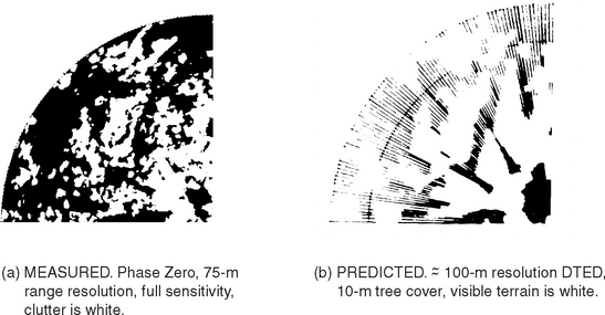
FIGURE 2.11 Measured and predicted clutter visibility in the northwest quadrant at Katahdin Hill. Maximum range is 12 km, north is zenith.
This relatively good correspondence between predicted terrain visibility and clutter occurrence at Katahdin Hill is further illustrated by the results shown in Chapter 4, Figure 4.2. However, careful observation reveals that significant (black) microshadowing occurs within visible regions in Figure 2.11 where the radar is at its noise floor. That is, at low illumination angles (∼0.5° in Figure 2.11) over hilly forested terrain it is not possible to predict every microshadowed cell. The theoretical probability distributions as developed herein for prediction of clutter statistics within visible regions include weak clutter values in the correct proportions by terrain type and illumination angle to correctly account for the microshadowing that occurs in the measurements. This matter is taken up again in Section 2.4.4.1 (see Figure 2.46), and in Chapter 4, Section 4.4 (see also the relevant discussion on phenomenology concluding Section 2.4.2.1).
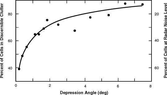
FIGURE 2.46 General incidence of microshadowing within clutter patches as a function of depression angle. Phase Zero X-band data, 75-m range resolution, horizontal polarization, 2- to 12-km range. All terrain types, 1,926 patches from 86 sites. Each plotted point represents the overall percentage of all cells from all patches at a given depression angle.
Tree Lines. Tree lines constitute dominant clutter sources on much composite landscape. Figure 2.12 shows backscatter from one particular tree line measured at relatively long range, 14.7 km, over intervening farmland at Gull Lake East. The data in Figure 2.12 show that, in the transition region between farmland and forest, a very strong specular-like return is received from the leading edge of the tree zone, which rapidly decays in the next few range gates as the wavefront penetrates further into the forest. The trees of this forest are predominantly aspen. The backscatter from the edge of the forest is from the beginning of a tree foliage zone (largely leaves and branches) rather than a line of trunks. Figure 2.13 shows Phase Zero backscatter from another tree line measured at much closer range at the Lincoln Laboratory outdoor antenna range at Bedford, Massachusetts. Here again a strong return is evident from the leading edge of the trees in the transition zone between the level grass (of the antenna range) and the forest, which rapidly decays with increasing penetration of the wavefront into the forest.
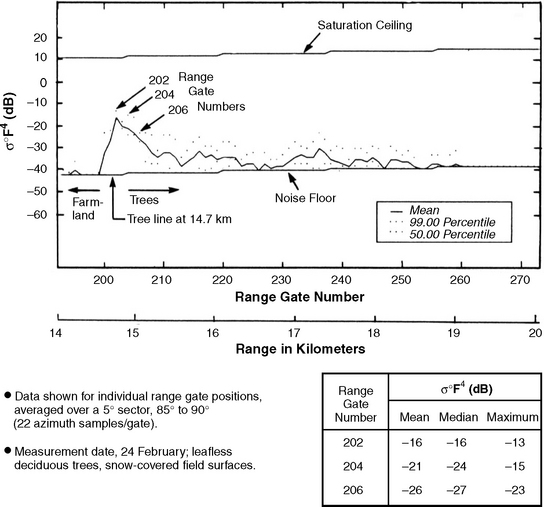
FIGURE 2.12 Backscatter from a tree line at 15-km range at Gull Lake East, Manitoba. Phase Zero X-band data, 75-m range resolution, horizontal polarization, 23.5-km maximum range, 74.2-m sampling interval.
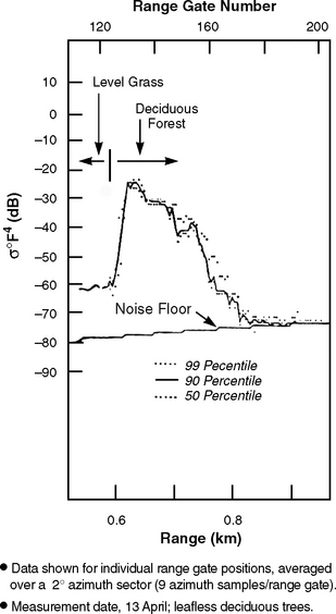
FIGURE 2.13 Backscatter from a tree line at Bedford, Massachusetts. Phase Zero X-band data, 9-m range resolution, horizontal polarization, 1.47-km maximum range setting, 4.6-m sampling interval.
Step Discontinuity. A theoretical problem directly relatable to low-angle clutter is backscattering from a dielectric step discontinuity at grazing incidence [8], as is illustrated in Figure 2.14(a). A solution to this problem consisting of a strong impulse-like leading edge return followed by a subsequent decay is of more direct applicability to low-angle clutter than one attempting to deal with low-angle clutter as an extended continuous surface. A Poisson distribution of many such discrete landscape elements leads to a K-distribution of clutter amplitudes [9] similar to the empirical Weibull distributions of this book.

Generality vs Specificity. Patch 20 at Gull Lake West occurs at the edge of Lake Winnipeg and largely comprises open water in which the ground clutter sources are shrub-covered sandy bars illuminated at a depression angle of ≈0.7°. The clutter amplitude distributions for patch 20 shown in Figure 2.9 are characterized by extreme spread. These distributions are very similar to distributions measured at much lower depression angles, typically at 0.1° or 0.2°, from cropland. The reason that patch 20 at higher angle looks like cropland at lower angle is that, in both cases, there exists a relatively low incidence of discrete clutter sources of widely varying strength rising above a low-backscattering medium. Patch 20 illustrates a general point in ground clutter modeling. With ever increasing detail and specificity in terrain description (e.g., the key to the unusualness of patch 20 is its land cover classification), prediction accuracy can be improved, but at the same time generality and simplicity—essential features of any model—are lost. Taken to the extreme, every measured patch is different (terrain is essentially infinitely variable) and an archival file of many specific measurements does not constitute a model. An objective of Chapter 2 is to develop simple general clutter modeling information that is not too demanding in terms of terrain representation but correctly presents fundamental trends in clutter statistics. Such a model will of necessity lack specificity in terrain representation—it will not predict every clutter patch exactly correctly, but over many patches and many sites it will exhibit correct general trends.
2.3.4 DEPRESSION ANGLE
Figure 2.15 shows depression angle α to be the angle below the horizontal at which a clutter patch is observed at the radar (see also Figure 2.5). More specifically, depression angle is defined herein to be the complement of incidence angle at the terrain point under consideration. Incidence angle equals the angle between the projection of the earth’s radius at the terrain point and the direction of illumination at that point, assuming a 4/3 earth radius to account for nominal atmospheric refraction. Thus the rigorous definition of depression angle is in a reference frame centered at the terrain point, not at the antenna. This definition of depression angle includes the effect of earth curvature on the angle of illumination, but does not include any effect of the local terrain slope.
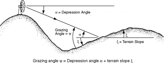
What is thusly referred to herein as “depression angle” has occasionally in the past been referred to as “grazing angle,” especially with airborne radar looking at long ranges over the spherical earth such that earth curvature effects are large (e.g., see [5], p.36). However, as shown in Figure 2.15, grazing angle as used herein refers to the angle between the tangent to the local terrain surface at the backscattering terrain point and the direction of illumination. Thus grazing angle as used herein does take into account the local terrain slope. The effects of grazing angle on clutter strength are discussed more fully in Section 2.3.5.
The formula used for rigorous computation of depression angle α is derived in Appendix 2.C to be
where h = effective radar height, r = slant range from radar to terrain point, and a = effective earth’s radius (actual earth’s radius times 4/3 to account for standard atmospheric refraction). At short enough ranges that earth curvature is insignificant, which is the case for much of the data in Chapter 2, Eq. (2.1) for depression angle simplifies to be α ≅ h/r; i.e., to be the angle below the horizontal at which the terrain point is viewed from the antenna. Figure 2.16 shows three clutter histograms which together illustrate the major effect of depression angle on histogram shape, such that variations with depression angle—i.e., as it ranges from 2.8° [Figure 2.16(a)] to 0.8° [Figure 2.16(b)] to 0.2° [Figure 2.16(c)]—tend to wash out other variations such as those that occur with changing landform and land cover. Note that the mean strengths (dashed vertical lines) in these three histograms vary by only several dB; it is the shapes and resultant spreads (e.g., ratios of 99-to 50-percentile) in these results that vary more dramatically with small changes in depression angle. In what follows, effects with depression angle on both mean strength and spread are discussed in low and high angle regimes.

FIGURE 2.16 Histograms of Phase Zero clutter amplitude statistics for three clutter patches at different depression angles. (a) High Knob, dep. ang. = 2.8°; (b) Orion, dep. ang. = 0.8°; (c) Coaldale, dep. ang. = 0.2°.
2.3.4.1 LOW-ANGLE CLUTTER
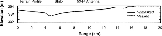
To illustrate the effect of depression angle on low-angle clutter, results are shown from two sites. First, results are shown from Shilo, Manitoba at a very low depression angle, 0.1° or 0.2°. Then results are shown from Cazenovia, New York at a much higher depression angle of ∼9°. In contrast to Gull Lake West, which was wooded terrain with occasional agricultural fields, the terrain at Shilo was open prairie farmland. Terrain relief at Shilo was low, less than 50 m over 10- to 20-km extents. The site position itself provided little elevation advantage over surrounding terrain. A terrain elevation profile to the southwest at Shilo is shown in Figure 2.17, incorporating the curvature of a 4/3 radius spherical earth. Geometrical masking is also shown in this figure. In this southwest terrain profile, the depressional dip at about 4.5-km range is a river valley. From 5.2 to 13.4 km, the terrain gradually rises out of the river valley at an average terrain slope of 0.26°. Although this is a small angle, it is more than sufficient to bring this terrain into full visibility from the radar position. Small changes in terrain slope to the southwest at Shilo, for example, in the regions from 13.4 to 15.1 km and beyond 17.3 km, are enough to cause these regions to be masked, which leads to an important point that is often misconstrued at first consideration. Terrain slope and changes in terrain slope, even when quite small, are very important in how they directly and deterministically affect the spatial patterns of occurrence of the clutter. The effect of terrain slope on clutter strength, however, is an entirely different matter, which is discussed in Section 2.1.5.
σ° vs Range. Figure 2.18 shows clutter strength vs range in a narrow azimuth sector to the southwest at Shilo. The available dynamic range between the noise floor and the saturation ceiling of the Phase Zero receiver is shown in the figure. Only in the first 2 km on the relatively discrete-free prairie grassland that exists in this near-in region is seen anything approaching a traditional deterministic effect between area-extensive σ° from the terrain surface itself and grazing angle. This close to the radar, the antenna mast height is sufficient to provide grazing angles greater than 0.5°. Thus as range decreases from 2 km, grazing angle increases from 0.5 degrees, and clutter strengths rise. Even in this near-in region, the nature of the increase of σ° with grazing angle is not smooth and monotonic but shows wide fluctuations.

FIGURE 2.18 Clutter strength vs range to the southwest at Shilo, Manitoba. Phase Zero X-band data, 11.8-km maximum range experiment, 75-m range resolution.
Beyond 2 km, the clutter strengths in Figure 2.18 are dominated by discrete clutter sources. This is evident in Figure 2.19, which shows a sector of a measured 12-km Phase Zero ground clutter map looking to the southwest at Shilo, overlaid and registered on an aerial photograph of the site. The agricultural fields within this sector are within geometric line-of-sight of the radar and are thus under direct illumination. Yet it is evident in Figure 2.19 that the radar is not sensitive to the backscatter from the field surfaces themselves. Rather, the clutter sources in these fields are all vertical discrete objects, including individual farmsteads (usually surrounded by trees) and other vertical features such as fence lines, telephone poles, bushes, and buildings.

FIGURE 2.19 A sector of ground clutter at Shilo, Manitoba. Within the sector, microregions of terrain generating discernible Phase Zero clutter are circumscribed with a heavy black line. Within each such microregion, some vertical feature can be identified in the air photo. Much of the area within the sector, including most open field surfaces, is at the Phase Zero noise floor (i.e., not circumscribed). The radial extent of the sector shown is 12 km.
The overall nature of the low-angle clutter amplitude phenomenon shown in Figure 2.18 shows extreme and rapid variation of clutter strength from range gate to range gate. These variations easily encompass 30 dB or more at a given percentile level of strength. The overall picture is not one of well-behaved or easy-to-describe statistics. Rather, it is one of patchiness and heterogeneity. The effects shown are not capturable in a traditional grazing angle model based on terrain slope. This, however, is the phenomenon, highly terrain-profile-specific and discrete-dominated, that requires characterization.
2.3.4.2 HIGHER-ANGLE CLUTTER
Consider now clutter strength vs range data from a much higher site, Cazenovia, New York. At Cazenovia the radar was set up high on the side of a steep valley, as shown in the top sketch in Figure 2.20. The radar looked down into the valley at high airborne-like depression angles. Beneath the terrain profile in Figure 2.20 are σ°F4 data vs range shown in the same manner as in Figure 2.18 for Shilo, averaged azimuthally over an azimuth sector in individual range gate positions. The dashed lines between the upper terrain profile and the lower clutter data trace are included merely to aid the eye in associating particular points within the data window on the terrain profile with corresponding points in the clutter data.

FIGURE 2.20 Clutter strength vs range at a high depression angle at Cazenovia, NY. Phase Zero X-band data, 3-km maximum range experiment, 9-m range resolution.
The data in Figure 2.20 seem to belong to a completely different phenomenological regime than the data in Figure 2.18. At the higher depression angle, the fluctuations of clutter strength with range are much less, more on the order of 6 dB than the 30-dB swings shown in Figure 2.18. The variation of clutter strength with range at high depression angle in Figure 2.20 is much less patchy, more homogeneous, and gives much more indication of being of a continuous process rather than being like the discrete-dominated process of Figure 2.18. The amount of shadowing (i.e., noise level cells) is dramatically reduced (essentially to zero) from Figure 2.18 to Figure 2.20. Thus, the most remarkable feature in the high-angle data of Figure 2.20 is the reduction of spread in clutter amplitudes exhibited at the higher illumination angle. Besides reduction in spread, the mean clutter strength has increased with depression angle also, from about σ°F4 ∼ −33 dB in Figure 2.18 to about σ°F4 ∼ −24 dB in Figure 2.20. These two major effects of decreasing spread and increasing mean strength in clutter amplitude distributions as depression angle increases and shadowing decreases are basic effects around which is formulated the preliminary X-band clutter modeling information of Chapter 2.
Next consider more closely the clutter data in Figure 2.20. The terrain on the valley floor is agricultural, with some scattered trees in wood lots, around farmsteads, and along roads. As the terrain slopes increase on the valley walls, however, the terrain becomes more completely forest covered. The effects of these variations in land cover are seen in the clutter data of Figure 2.20. There is more fluctuation in clutter strength from the farmland on the valley floor between 1.0 and 1.5 km in range. From the forested surfaces, between 0.75 and 1.0 km and between 1.75 km and 2.25 km, there is less fluctuation, and the amplitude distributions become close to Rayleigh.
Grazing Angle. Also shown in Figure 2.20 is an approximate indication of grazing angle. A traditional way to model higher angle ground clutter is by means of a constant-γ model, where clutter strength varies directly with the sine of the grazing angle, the constant of proportionality being γ (see Section 1.2.5). The mean clutter strength data in Figure 2.20 show rises and drops with changing grazing angle, with each of the changes being of about the expected 2- or 3-dB order of magnitude. Thus the data of Figure 2.20 support a constant-γ grazing angle model for mean clutter strength at high angle as being quite realistic. The value of γ suggested by the data of Figure 2.20 is 0.023 (i.e., −16.4 dB), with γ being somewhat independent of terrain type, a conclusion supported by the airborne SAR clutter measurements discussed in Section 2.4.4.2. However, the grazing angles of Figure 2.20 are so high as to be much more typical of airborne radar than general ground-based radar. Certainly a constant-γ model has no applicability to the lower angle regimes of ground-based radar exemplified by the Shilo data and which constitute the major subject of this book. The data of Figure 2.20 indicate what kind of an unusual terrain geometry is required in a ground-based measurement for grazing angle and constant-γ to be useful.
It is only because of its closeness (< ∼2 km) that visibility exists into the deep Cazenovia valley at all. Similar valleys at longer ranges are typically screened to ground-based radar. Still, consideration of the Cazenovia data of Figure 2.20 within the context of the preliminary clutter modeling information presented later in Chapter 2 provides a better indication of how the model works and the terrain scale at which it is meant to work. Although the very local close-in data of Figure 2.20 can be analyzed through grazing angle, the subsequent model works more globally and to much longer ranges, utilizing large terrain patches characterized in terms of terrain relief (i.e., terrain slope) and depression angle.
Only in special circumstances, such as looking down into and across a single deep linear valley at close range such as occurs at Cazenovia, are direct and specific causative influences of grazing angle on clutter strength in surface radar able to be shown. Consider again backscatter from a step discontinuity as shown in Figure 2.14. At very low angles of illumination [i.e., Figure 2.14(a)], vertical surfaces are illuminated at normal incidence and give rise to strong returns, whereas horizontal surfaces are illuminated at grazing incidence and give rise to weak returns. This is the situation prevailing in the Shilo data. However, at higher angles of illumination [i.e., Figure 2.14(b)], both vertical and horizontal surfaces are illuminated at angles in between normal and grazing and give rise to returns of more nearly equivalent strength. This is the situation prevailing in the Cazenovia data. That is, at the higher angles of the constant-γ regime, vertical features are less obtrusive and tend to “melt into” the horizontal background.
2.3.5 TERRAIN SLOPE/GRAZING ANGLE
Depression angle does not depend on the local terrain slope at the backscattering terrain point, whereas grazing angle, defined to be the angle between the tangent to the local terrain surface at the backscattering terrain point and the direction of illumination, does depend on the local terrain slope (see Figure 2.15). If depression angle is a useful modeling parameter of low-angle clutter, should not grazing angle be a better parameter? Intuition strongly suggests that the best measure of illumination angle in considering backscattering from a rough surface is the angle between the direction of illumination and the plane of the surface.
Discrete vertical land cover features often dominate as clutter sources in low-angle clutter. For example, if a tree exists in a spatial resolution cell, the slope of the ground under the tree is not very significant in affecting the backscatter from the cell. Trees and other vertical landscape features are vertical irrespective of the underlying terrain slope. Thus discrete land cover features, which are the dominant low-angle clutter sources, act to emphasize depression angle and de-emphasize grazing angle as the fundamental measure of illumination angle.
2.3.5.1 DIGITIZED TERRAIN ELEVATION DATA
Set aside for the moment the issue of discrete vertical features in land cover—assume that terrain slope will act as a dominant parameter strong enough to overcome such dispersive effects in low-angle clutter. How should these important terrain slopes be computed or measured? At this point, consider the availability of digitized terrain elevation data (DTED) from various sources. Such DTED are provided as points of terrain elevation of specified vertical precision (e.g., ∼1 m) on a horizontal latitude/longitude grid of specified sampling interval (e.g., ∼100 m). In clutter modeling, can grazing angle be usefully brought to bear to predict clutter strength, cell by cell in the DTED, based on the elemental terrain slopes provided by these data? If such an approach were successful, the DTED could carry the burden of describing terrain, which is a root cause of difficulty in clutter modeling. A clutter model could then be a simple relationship between cell-level grazing angle and clutter strength.
σ° vs Grazing Angle. An example of cell-level correlation between measured clutter strength and DTED-predicted grazing angle is shown in Figure 2.21. The site for which the data of Figure 2.21 apply is Brazeau, a forested site of significant relief in Alberta, Canada. Selection of a forested site provides a more spatially continuous scattering medium and minimizes the effects of strong discretes such as occur on more open landscapes, thus potentially giving grazing angle a better chance to work.15 For each resolution cell within 20-km maximum range at Brazeau, terrain slope and grazing angle were computed from DTED and registered with the measured Phase Zero clutter strength for the cell. Then, for each cell that was within geometric visibility and for which the Phase Zero radar measured a discernible clutter return, a single point was plotted in Figure 2.21. Doing so for all such points resulted in the scatter plot shown.
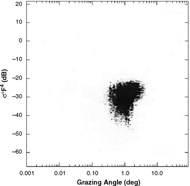
FIGURE 2.21 Cell level scatter diagram of measured σ°F4 vs grazing angle at Brazeau, Alta. Range interval = 1 to 20 km. Azimuth interval = 1.0° to 360°. Phase Zero X-band clutter data, horizontal polarization, 75-m range resolution. Terrain slope at each cell computed from digitized terrain elevation data (DTED).
Very little useful correlation is seen between clutter strength and grazing angle in Figure 2.21. The actual correlation coefficient computed for these data is 0.21. Scatter plots similar to Figure 2.21 were generated for six different sites of widely varying terrain type. The largest correlation coefficient obtained was 0.23. Negative correlation between grazing angle and clutter strength was equally likely to positive correlation. For one site, additional DTED of five-fold improvement in scale, precision, and accuracy were utilized with little improvement in the results. These investigations have shown the idea of a simple clutter model based on statistically significant direct correlation between cell-level estimates of grazing angle from DTED and measured clutter strength to be inefficacious. Such a simple model does not resolve the complexities of real terrain. Any usefulness in such correlative associations requires more sophisticated analyses looking for more subtle effects (see Appendix 4.D).
DTED Accuracy. Why is so little correlation seen between clutter strength and grazing angle predicted from DTED? First recall that DTED describes only a bare earth and contains no information describing land cover, the edges of land cover features, or other discrete land cover objects that dominate low-angle clutter. Beyond this, however, the results shown in Figure 2.22 provide more insight. These results apply to forested terrain in eastern Massachusetts. In Figure 2.22, terrain elevations are shown based on two sources,
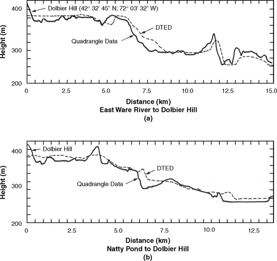
FIGURE 2.22 Terrain elevation profile along two paths in Massachusetts, comparing digitized terrain elevation data (DTED) and data derived from quadrangle topographic maps. The quadrangle-map-derived data are ∼10 times more accurate than the DTED.
(1) DTED and (2) quadrangle topographic maps. The quadrangle maps from which information was plotted directly in Figure 2.22 were of much higher precision and accuracy (by a factor of ∼10) than the DTED. The two terrain profiles in Figure 2.22, DTED and quadrangle, show general similarity. Consequently, use of DTED to predict macroscale regions of terrain visibility and shadow provides useful information. However, it is another matter to consider correlating local terrain slopes with clutter strength, cell by cell, in the data of Figure 2.22. Since the quadrangle data are more accurate, it is evident that many DTED cells provide markedly inaccurate estimates of terrain slope. Clearly such DTED do not contain precise and accurate enough information to provide terrain slope detail at the scale of radar transmission wavelength, which is the scale at which the mechanisms of electromagnetic backscattering take place. Nor, in fact, do the quadrangle data provide such necessary precision and accuracy, since any map is a simplification of reality. As has been observed elsewhere, “… in typical agricultural and rolling terrain … the grazing angle is not readily definable” [10]; and “it [is] difficult to define grazing angle over a non-flat surface such as natural terrain” [6].
2.3.5.2 PATCH CLASSIFICATION BY TERRAIN SLOPE
The discussion now returns to the implicit idea that, at some level or some scale, terrain slope must strongly affect clutter strength. In contrast to DTED cells, consider the Phase Zero clutter patches, typically sized to be several kilometers on a side. Such patches are macroscale in comparison with microscale DTED cells. Recall that the landform within each patch is classified through interpretation of stereo aerial photographs and topographic maps. In this classification, terrain slope is a principal criterion. Of course, any patch several kilometers on a side presents various slopes to the radar, so it is the distribution of slopes over each patch that must be considered. This distribution of slopes over a patch depends on the measurement scale employed—increasing magnification always reveals increasing detail and new structure in the surface (i.e., fractal phenomenon). Thus the actual distribution of slopes over a patch is regarded as an indeterminate quantity.
Mean Clutter Strength By Landform. Through subjective interpretation of air photos and maps, bounds or limits may be set to the slopes existing within each patch, and subsequent binning of patches can occur within classes defined by these slope limits. Figure 2.23 specifies six categories of landform in increasing order of terrain slope. Within the category of level terrain, there exist Phase Zero measurements from 524 different patches. For each level patch, there exists a corresponding measured mean clutter strength. Figure 2.23 shows the cumulative distribution of mean clutter strength from all 524 patches of level terrain. Wide spread exists in this distribution of mean clutter strength measured from level patches. From maximum to minimum measured mean values, there is over 30 dB of variation. The cumulative distributions of mean clutter strength from the five remaining terrain types are also shown. If, as a measure of centrality, the median level (indicated by the horizontal dashed line) is selected in each distribution of mean clutter strength in Figure 2.23, a statistically significant monotonic increase in mean clutter strength with terrain slope is observed. That is, at the median level the distributions are displaced increasingly to the right with increasing terrain slope over a range of 11 dB from minimum to maximum. Hence intuition is justified. These data unequivocally illustrate that clutter strength depends on terrain slope. The effect is strong enough to be observed through dispersive influences of land cover, terrain heterogeneity, and depression angle. Two other important facts are also observed: (1) there is much spread within the distribution of mean clutter strength for any given class of landform, and (2) although significant, there is relatively little separation between adjacent classes.

FIGURE 2.23 Cumulative distributions of mean ground clutter strength by landform in rural terrain. Phase Zero X-band data, 75-m range resolution, horizontal polarization, 2- to 12-km range, 1809 patches, 96 sites. Each curve shows the cumulative distribution of mean clutter strengths from all patches of a given terrain type, one value of mean strength per patch.
Mean Clutter Strength By Land Cover. Similar to the way in which Figure 2.23 shows how Phase Zero mean clutter strengths separate in six classes of landform, Figure 2.24 shows how Phase Zero mean clutter strengths separate in six classes of land cover. As might be intuitively expected, the data of Figure 2.24 indicate that, in terms of mean clutter strength, urban terrain is stronger and wetland weaker than most other land cover types. The expected-value results in Figures 2.23 and 2.24 are derived from the same set of 2,177 Phase Zero clutter patch measurements described earlier.

FIGURE 2.24 Cumulative distributions of mean ground clutter strength by land cover. Phase Zero X-band data, 75-m range resolution, horizontal polarization, 2- to 12-km range, 2,172 patches, 96 sites. Each curve shows the cumulative distribution of mean clutter strengths from all patches of a given terrain type, one value of mean strength per patch.
2.3.6 CLUTTER MODELING
Assume that DTED are available for the site to be modeled. The DTED can be used to define kilometer-sized clutter patches as regions of general geometric visibility. This is an appropriate use of DTED, well matched to the information content of the database. Within these macroregions of visibility, clutter strength cannot be accurately predicted cell by cell simply by association with the local terrain slope and grazing angle at the cell. This is an inappropriate use of DTED because the sought-after information is at a scale, accuracy, and precision not contained within the data.
Still, illumination angle is of major importance in its effects on low-angle clutter strength. Rather than grazing angle, results in this book are based on depression angle. Depression angle is a quantity that can be computed relatively rigorously and unambiguously from available information. For example, within a macropatch of visible terrain in DTED, depression angle—which depends only on the cell-level elevations over the patch and not the detailed rates of change of these elevations—is a quantity that varies relatively slowly over the patch. If the mean depression angle over the patch is computed, this mean value is relatively insensitive to the questions of accuracy, precision, and scale that plague grazing angle.
But in using depression angle, how are the important effects of terrain slope incorporated? Reconsider the data in Figure 2.23 that statistically show how mean clutter strength increases with terrain slope. As shown there, terrain is simply separated into two categories, low and high relief. Low-relief terrain provides slopes of < 2°; high-relief terrain provides slopes of > 2°. Thus in Figure 2.23, level, inclined, and undulating terrain categories are all low relief; whereas rolling, moderately steep, and steep terrain categories are all high relief. This simple landform-descriptive scheme consisting of two relatively general classes captures much of the statistical significance in the dependency of clutter strength on terrain slope, given the large spread within and little separation between more specific classes. In addition, this simple twofold scheme has the attendant advantage of liberating the user of these results from providing highly detailed descriptions of terrain.
Superficially, it may appear that terrain slope enters the current results only through specification of terrain relief as low or high. However, the further quantitative dependence of these results on depression angle also carries with it an implicit dependence on terrain slope, wherein higher terrain slopes generally occur at higher depression angles (i.e., high sites usually occur in hilly terrain). Thus, results in this book take into account terrain slope, not in simplistic or idealized ways, but in practicable ways that have stood the test of trial in the empirical data.
2.4 X-BAND CLUTTER SPATIAL AMPLITUDE STATISTICS
Section 2.4 provides modeling information for predicting ground clutter amplitude statistics applicable to spatial distribution over patches of visible terrain as seen by a surface-sited X-band radar. This information is arrived at by combining measurements from many similar Phase Zero patches into ensemble distributions of clutter amplitude statistics. By the word “similar” is meant patches of like-classified terrain that are viewed at closely similar depression angles. Section 2.4 provides clutter strength modeling information for both general and various specific levels of terrain classification.
Modeling information is presented in Section 2.4 within a standard tabular format involving (1) terrain type, (2) depression angle, (3) Weibull coefficients of the approximating Weibull amplitude distribution, (4) measured mean strength of the ensemble amplitude distribution, (5) the percent of microshadowed cells (i.e., percent of cells at radar noise level)16 within the ensemble distribution, and (6) the number of clutter patches included in the ensemble. The three Weibull coefficients presented are the Weibull shape parameter aw, the Weibull median clutter strength ![]() , and the Weibull mean clutter strength
, and the Weibull mean clutter strength ![]() . The important characteristic of spread in the approximating Weibull distribution is observable, either directly in the aw parameter, or in the mean-to-median ratio.
. The important characteristic of spread in the approximating Weibull distribution is observable, either directly in the aw parameter, or in the mean-to-median ratio.
The modeling information in Section 2.4 illustrates the first important trends discovered in the Phase Zero data—namely, the dependencies of ![]() and aw on depression angle. The information provided for aw is limited to Phase Zero spatial resolution (i.e., 1° azimuth beamwidth and, generally, 0.5 μs pulse length; but see also Section 2.4.5). More general effects of resolution on aw are developed in following chapters. The important trends of
and aw on depression angle. The information provided for aw is limited to Phase Zero spatial resolution (i.e., 1° azimuth beamwidth and, generally, 0.5 μs pulse length; but see also Section 2.4.5). More general effects of resolution on aw are developed in following chapters. The important trends of ![]() and aw with depression angle observed to occur in the preliminary X-band modeling information of Section 2.4 also occur at other spatial resolutions, but the precise numbers specifying aw vary with the resolution of the radar under consideration.
and aw with depression angle observed to occur in the preliminary X-band modeling information of Section 2.4 also occur at other spatial resolutions, but the precise numbers specifying aw vary with the resolution of the radar under consideration.
2.4.1 AMPLITUDE DISTRIBUTIONS BY DEPRESSION ANGLE FOR THREE GENERAL TERRAIN TYPES
Specified here are spatial amplitude distributions of low-angle X-band ground clutter for three general terrain types: (1) rural/low-relief, (2) rural/high-relief, and (3) urban. These three terrain types are summarily described in Table 2.3. These terrain types are all-inclusive—any patch of terrain must be classified as one and only one of these three types. Thus rural terrain includes such diverse specific terrain types as agricultural, forest, rangeland, wetland, and barren. Urban terrain includes any kind of built-up land such as commercial, industrial, and residential. In terms of degrees of roughness of terrain surface, the classification system utilized (see Table 2.2) incorporates the following specific categories: level, undulating, hummocky, inclined, broken, rolling, ridged, moderately steep, and steep. Low relief encompasses the first five categories, and high relief encompasses the last four. Note that the actual distribution of slopes that exists within a macroscale clutter patch is specified, not the overall slope of the best-fit plane through the patch.
TABLE 2.3
| 1 | Rural/Low-Relief |
| (Slopes < 2°; Relief < 100 ft) | |
| 2 | Rural/High-Relief |
| (Slopes > 2°; Relief > 100 ft) | |
| 3 | Urban |
In data reduction and analysis, X-band clutter amplitude distributions were formed from 2,177 Phase Zero clutter patches, each generally several kilometers on a side. For each patch, detailed terrain descriptions at the specific level just described were determined. It was found that in the separation of clutter amplitude data into such specific terrain-descriptive classes, spread within class was broad and separation between similar or neighboring classes was narrow. Thus the three general terrain classes of Table 2.3 are utilized, which do provide significant and useful separation of X-band clutter data. A simple way of interpreting these three general terrain types is that only “mountains” (rural/high-relief) and “cities” (urban) grossly warrant separation from all other terrain types (rural/low-relief).
Empirical ground clutter spatial amplitude distributions are presented in Figure 2.25 by depression angle for rural/low- and rural/high-relief terrain. Similar results are presented in Figure 2.26 for urban terrain (in which the regime of the rural distributions is shown lightly shaded for comparison). These distributions include all spatial samples within patches including cells at radar noise level, but are shown only over σ°F4 regimes to the right of the highest noise-contaminated bin. Thus, where shown, these distributions are independent of Phase Zero sensitivity and represent what a theoretically infinitely sensitive radar would measure.

FIGURE 2.25 Cumulative ground clutter amplitude distributions by depression angle for rural terrain of low- and high-relief. Phase Zero X-band data, 75-m range resolution, horizontal polarization, 2- to 12-km range, 1,743 patches, 87 sites.

FIGURE 2.26 Cumulative ground clutter amplitude distributions by depression angle for urban terrain. Phase Zero X-band data, 75-m range resolution, horizontal polarization, 2- to 12-km range, 109 patches, 33 sites.
It is seen that, within each of these three terrain types, the shape of the spatial amplitude distribution is strongly dependent on depression angle, such that there is a continuous rapid decrease in the spread of the distribution with increasing depression angle, even over the very small depression angles (usually < 1.5° in low-relief terrain) associated with surface-sited radar. The distributions in Figures 2.25 and 2.26 are formed by combining like-classified clutter data from a large data set altogether comprising 2,177 clutter patch amplitude distributions obtained from measurements at 96 sites at ranges from 2- to 12-km from the radar. It is only by means of such extensive averaging that the smooth monotonic dependence of both strength (the distributions gradually move to the right with increasing angle) and spread (the slopes of the distributions gradually increase with increasing angle) emerge in these empirical distributions to provide a general predictive capability. These underlying fundamental trends are often obscured by specific effects in individual measurements.
Most (66%) of these measured data are contained in the rural/low-relief distributions of Figure 2.25. It is this parametric regime that is applicable to most surface radar situations and has traditionally been least well understood. The set of rural/low-relief distributions is extended in the rural/high-relief distributions (the latter accounting for 18% of the data), where higher depression angles are realized in high-relief terrain through higher site locations. Across the rural data set as a whole, the effect of continuously decreasing spread in the distributions with increasing angle is at the heart of understanding low-angle clutter as a physical phenomenon dominated by microshadowing. The highest angle distribution (6° to 8° depression angle) almost achieves the Rayleigh slope, reflecting the fact that the amount of microshadowing is relatively small at such high airborne-like angles. The resultant nearly full illumination, as expected, provides approximately Rayleigh statistics. The urban distributions of Figure 2.26 (which contain 6% of the measured data) also show monotonically decreasing spread with increasing angle, but contain significantly stronger clutter than the corresponding rural/low-relief distributions. Ten percent of clutter patches were measured at negative depression angles; these data are discussed in Section 2.4.2.6.
Depression Angle Distributions. The distributions of depression angle at which Phase Zero clutter patches were measured are shown in Figure 2.27, both as an overall distribution and separated into rural/low-relief, rural/high-relief, and urban components. Depression angle is a fundamental parameter in low-angle clutter. It is the distributions shown in Figure 2.27, partitioned into appropriate contiguous intervals, that exert controlling influence on the distributions in Figures 2.25 and 2.26. In each part of Figure 2.27, cumulative probability is given by the s-shaped curve and read on the left ordinate; percentage of patches is given by the underlying histogram and read on the right ordinate. The data in Figure 2.27 indicate that depression angles to visible terrain for surface-sited radars are usually quite low, but the data also show that depression angles in high-relief terrain range over significantly higher values than those in low-relief terrain. The single highest depression angle at which a Phase Zero clutter patch was measured was 13.8° at the Equinox Mountain site in Vermont. The largest negative depression angle at which a Phase Zero clutter patch was measured was −4.4° at the Waterton site in Alberta.

FIGURE 2.27 Distributions of depression angle at which clutter patches were measured. Phase Zero measurements, 96 sites, 2- to 12-km range.
2.4.1.1 WEIBULL PARAMETERS
The cumulative clutter amplitude distributions shown in Figures 2.25 and 2.26 are relatively linear as plotted on the Weibull probability scale of these figures, and thus can be usefully approximated with Weibull statistics (a theoretical Weibull distribution plots as a straight line in these figures). The Weibull distribution is discussed in Appendix 2.B, including the methodology utilized for obtaining Weibull approximations to measured distributions. Weibull distributions provide the wide degree of spread appropriate to low-angle ground clutter amplitude distributions. The Weibull cumulative distribution function may be written [11, 12]:
where
The mean-to-median ratio for Weibull statistics is
where ![]() is the mean value of x and Γ is the gamma function. Here the random variable x represents clutter strength σ°F4 including propagation effects.
is the mean value of x and Γ is the gamma function. Here the random variable x represents clutter strength σ°F4 including propagation effects.
Section 2.4 characterizes measured Phase Zero empirical clutter amplitude distributions by means of the two Weibull coefficients, the Weibull shape parameter aw, and the decibel value of Weibull median clutter strength ![]() (dB). These two coefficients entirely characterize the modeled distribution; from them the distribution can be easily visualized or sketched, and Weibull random numbers belonging to the modeled distribution can be generated. The Weibull shape parameter aw is a dimensionless quantity indicative of the spread of the distribution. For aw = 1, the Weibull distribution degenerates to a Rayleigh17 distribution, which represents a lower bound on spread in clutter spatial amplitude statistics. Most of the Phase Zero empirical spatial amplitude distributions are approximated by values of shape parameter such that aw > 1.
(dB). These two coefficients entirely characterize the modeled distribution; from them the distribution can be easily visualized or sketched, and Weibull random numbers belonging to the modeled distribution can be generated. The Weibull shape parameter aw is a dimensionless quantity indicative of the spread of the distribution. For aw = 1, the Weibull distribution degenerates to a Rayleigh17 distribution, which represents a lower bound on spread in clutter spatial amplitude statistics. Most of the Phase Zero empirical spatial amplitude distributions are approximated by values of shape parameter such that aw > 1.
In addition, Section 2.4 provides ![]() (dB), the decibel value of Weibull mean strength in the modeled distribution. The Weibull mean strength
(dB), the decibel value of Weibull mean strength in the modeled distribution. The Weibull mean strength ![]() (dB) is provided to compare with the mean strength in the actual measured ensemble distribution as a first measure of goodness-of-fit of the Weibull model to the measured data. The spread in the approximating distribution may also be assessed by the mean-to-median ratio,
(dB) is provided to compare with the mean strength in the actual measured ensemble distribution as a first measure of goodness-of-fit of the Weibull model to the measured data. The spread in the approximating distribution may also be assessed by the mean-to-median ratio, ![]() (dB) minus
(dB) minus ![]() (dB). Median levels of the actual measured ensemble distributions may be read or estimated from their graphed cumulative distributions. As mentioned in Section 2.3.3.2, almost none of the measured distributions pass rigorous statistical hypothesis tests for Weibull on any other analytically representable statistical distribution that was tried (but see Appendix 5.A, Section 5.A.4).
(dB). Median levels of the actual measured ensemble distributions may be read or estimated from their graphed cumulative distributions. As mentioned in Section 2.3.3.2, almost none of the measured distributions pass rigorous statistical hypothesis tests for Weibull on any other analytically representable statistical distribution that was tried (but see Appendix 5.A, Section 5.A.4).
Figure 2.28 shows five theoretical Weibull distributions plotted in the same manner as the empirical Phase Zero ensemble clutter amplitude distributions in Figures 2.25 and 2.26. All five of these theoretical distributions have the same median clutter strength, ![]() (dB) = −40, but have values of shape parameter aw ranging from aw = 1 to aw = 5. Comparison of similar percentile levels over these five distributions indicates their extreme differences. For example, for the distribution with aw = 5, one in a thousand samples is 50 dB stronger than
(dB) = −40, but have values of shape parameter aw ranging from aw = 1 to aw = 5. Comparison of similar percentile levels over these five distributions indicates their extreme differences. For example, for the distribution with aw = 5, one in a thousand samples is 50 dB stronger than ![]() (dB), whereas for the distribution with aw = 1 (the Rayleigh degenerative case), one in a thousand samples is only 10 dB stronger than
(dB), whereas for the distribution with aw = 1 (the Rayleigh degenerative case), one in a thousand samples is only 10 dB stronger than ![]() (dB). Clearly the shape parameter aw of a ground clutter spatial amplitude distribution strongly affects the false alarm statistics of a radar operating in that clutter. Use of Eq. (2.3) shows that the distribution for aw = 5 has mean strength
(dB). Clearly the shape parameter aw of a ground clutter spatial amplitude distribution strongly affects the false alarm statistics of a radar operating in that clutter. Use of Eq. (2.3) shows that the distribution for aw = 5 has mean strength ![]() dB whereas the distribution for aw = 1 has
dB whereas the distribution for aw = 1 has ![]() , which is 27 dB weaker.
, which is 27 dB weaker.
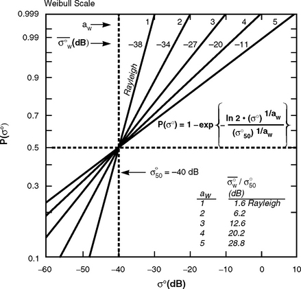
Specific Weibull approximations for the ground clutter amplitude distributions shown in Figures 2.25 and 2.26 are presented in Table 2.4 by depression angle for each of the three general terrain types. The table shows that large shape parameters at low angles rapidly diminish with increasing angle, approaching the Rayleigh value of unity at the highest angles. At the same time, median clutter strengths rapidly increase with increasing angle. Mean clutter strengths increase more gradually with increasing angle, so spread in terms of mean-to-median ratio is also observed to rapidly decrease with increasing angle. This behavior mirrors that of K-distributions (which also decrease in spread and degenerate to Rayleigh) which arise out of theoretical investigations of low-angle clutter amplitude distributions [13, 14]. To just describe these amplitude distributions, which is the intent here, Weibull distributions serve the purpose as well as K-distributions (see Appendix 5.A) and are simpler to use. The depression angle regimes are narrower and more numerous in Table 2.4 than in Figures 2.25 and 2.26, indicating that the parametric trend with depression angle is significant even for small steps of depression angle. The measured mean clutter strength for each ensemble distribution in the table is observed to closely match the mean strength of the approximating Weibull distribution, a first indication that laying a best-fitting Weibull straight line over central parts of each measured distribution of Figures 2.25 and 2.26 produces approximating distributions of reasonable mean strength. Table 2.4 strongly indicates that shadowing is a major cause of the variations that are observed with depression angle—the incidence of microshadowed cells varies from as much as 64% at grazing incidence in low-relief terrain to as little as 14% at high angle in high-relief terrain. The condensation and codification of properties of low-angle ground clutter within Weibull coefficients as presented in Table 2.4 fulfills much of what was initially sought to be understood about low-angle X-band ground clutter.

2.4.1.2 OVERALL DISTRIBUTION
Figure 2.29 shows the overall cumulative clutter amplitude ensemble distribution resulting from combining individual measurements from all 2,177 Phase Zero clutter patches into one distribution. This overall distribution is plotted cumulatively in Figure 2.29 on a Weibull probability axis that shows much more of the high (i.e., strong-side) tail of the distribution, up to 0.999999 on the probability axis, compared to the upper limit defined by 0.995 on the probability axis for the distributions shown in Figures 2.25 and 2.26.

FIGURE 2.29 Cumulative ground clutter amplitude distributions for rural/low-relief terrain, rural/high-relief terrain, urban terrain, and the overall combination of all three terrain types. Phase Zero X-band data, 75-m range resolution, horizontal polarization, 2- to 12-km range, 2,177 clutter patches. See also Table 2.5.
For cumulative probabilities below 0.995, the overall distribution is reasonably well fit by a linear Weibull approximation with shape parameter aw ≅ 3.9. However, this overall distribution has an upper tail at higher probabilities greater than 0.995, approximated by a much larger value of shape parameter. This upper tail of strong clutter values of increased spread compared with the central part of the distribution is due to occasional strong localized discrete scattering sources on the landscape such as water towers and grain storage elevators. Such objects are larger and of less frequent occurrence than the myriad smaller discrete objects acting as sources for the central part of the distribution. This high tail is relatively linear on the Weibull scale. The distribution of these relatively infrequent, widely ranging, strong clutter values, is thus well approximated for cumulative probability > 0.999 with Weibull shape parameter ![]() .
.
A Weibull fit to the central part of the overall distribution of Figure 2.29 represents the general spatial amplitude distribution of low-angle X-band land clutter, irrespective of depression angle and terrain type. The Weibull parameters of this general distribution are given in Table 2.5. The degree of linearity of the central part of the overall distribution in Figure 2.29 indicates that it is relatively well-fit by its Weibull approximation—this is borne out by the close comparison between the Weibull and actual ensemble mean clutter strengths in Table 2.5. In actuality, the central part of the overall distribution in Figure 2.29 is slightly concave upward, indicating that the exact shape of the distribution lies between that of a Weibull distribution and that of a K-distribution (see Appendix 5.A).
TABLE 2.5
Statistical Attributes of Rural/Low-Relief, Rural/High-Relief, Urban, and Overall Ground Clutter Amplitude Distributionsa
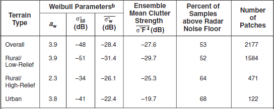
aPhase Zero X-band data, 75 m range res., hor. pol., 2 to 12 km range, 2177 patches. See also Figure 2.29.
bFor cumulative probability < 0.999
Rural/Low-Relief, Rural/High-Relief, Urban. Also shown in Figure 2.29 are the component ensemble distributions of the overall amplitude distribution corresponding to each of the three general terrain types: rural/low-relief, rural/high-relief, and urban. Statistical attributes for these three component distributions are also shown in Table 2.5. These three distributions may be used in non-site-specific ground clutter modeling to simply characterize the overall terrain at a site as one of these three general types. The increased spread in the high tail of the overall distribution caused by large discrete objects is mirrored in both the rural/low-relief and high-relief distributions in Figure 2.29.
At higher probabilities (> 0.9999) in the high tails, there is no distinction between the rural/low-relief and rural/high-relief distributions because large discrete objects cause these tails. The urban distribution also has a high tail with increased spread that extends to lower probability levels than do the high tails in rural terrain. The incidence of receiver saturation in the Phase Zero measurements is also shown in Figure 2.29. It is evident that the high-side tails in the distributions of Figure 2.29 are significantly affected by saturation, increasingly so with increasing clutter strength. These effects of saturation are to slightly under-estimate the high-side tails, which must extend to slightly higher strengths and be of slightly greater spread than indicated by the data of Figure 2.29. The effects of saturation are somewhat greater in the urban distribution in Figure 2.29—they cause an obvious break in slope in the urban high tail.
2.4.1.3 HIGH DISTRIBUTION TAILS
Having discussed the high tails in the overall ensemble clutter amplitude distributions, the discussion now turns to the high tails in the measured ensemble clutter amplitude distributions partitioned by depression angle. The high tails of the rural terrain clutter ensemble amplitude distributions of Figure 2.25 partitioned by depression angle are shown in Figure 2.30—the distributions by depression angle for low-relief terrain are shown in Figure 2.30(a), and those for high-relief terrain are shown in Figure 2.30(b).
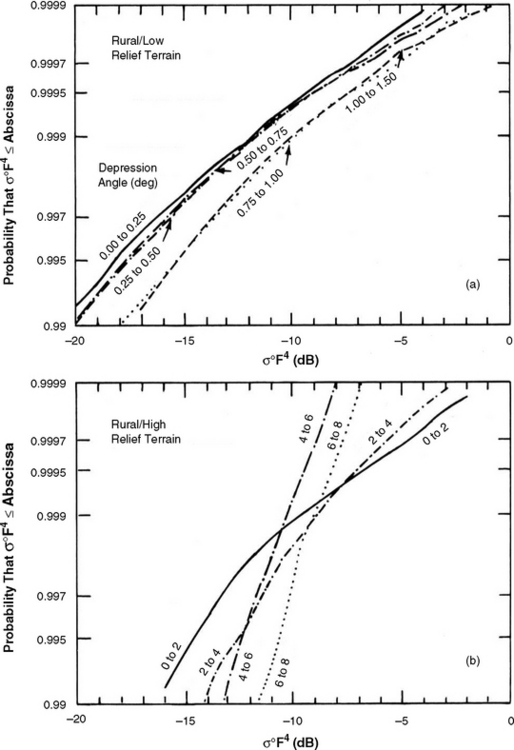
FIGURE 2.30 High tails of cumulative ground clutter amplitude distributions by depression angle for rural terrain of low- and high-relief. Phase Zero X-band data, 75-m range resolution, horizontal polarization, 2- to 12-km range, 1,743 patches, 87 sites. See also Figure 2.25.
Linear extrapolation of the distributions in Figure 2.25 to higher levels suggests a region of coalescence and possible crossover at higher probability levels. For low-relief terrain, Figure 2.30(a) shows that these distributions actually all roll to the right to assume the increased spread seen in the overall results of Figure 2.29, with little or no cross-over. For high-relief terrain, Figure 2.30(b) shows that the distributions for 0° to 2° and 2° to 4° also roll to the right with a crossover, but the distributions for 4° to 6° and 6° to 8° do not roll to the right but stay relatively linear on the Weibull scale to the highest probability levels shown.
These results indicate that at low angles in high-relief terrain large discrete objects are still evident, but that at high enough angles large discretes become much less evident. That is, at high angles in high-relief terrain, large discrete objects tend to “melt into” the background (as previously discussed, see Figure 2.14) so that it is much less probable to receive specular-like broadside flashes from discrete vertical objects at high angles in high-relief terrain than is the case at lower angles in high-relief terrain or in low-relief terrain in general. The high tails shown in Figures 2.29 and 2.30 are of interest because of their potential to cause false alarms in surface-sited radar operating in ground clutter.
2.4.2 CLUTTER RESULTS FOR MORE SPECIFIC TERRAIN TYPES
The basic Phase Zero ground clutter modeling information of Section 2.4.1 is based on three general terrain types. Although Weibull statistics and three terrain types are enough to show fundamental trends in low-angle clutter, the resultant basic construct cannot contain all the complex higher-order attributes of the actual phenomenon. Section 2.4.2 illustrates that increasing fidelity in terrain descriptive information can reveal higher-order trends in clutter statistics.
2.4.2.1 MOUNTAIN CLUTTER
Besides needing information describing general clutter strengths, an analyst may also need to know something about worst-case situations. Provided here is additional specific information on how strong mountain clutter can become.
Clutter Patches at Plateau Mountain. The steepest roughest terrain from which ground clutter was measured was that of the Canadian Rocky Mountains. One site, Plateau Mountain, was a flat-topped mountain site high in the Rockies that provided road access for the truck-borne clutter measurement equipment. From Plateau Mountain, the view to the west was of steep barren rock faces from high peaks in the Rockies. The lower slopes of these mountains were tree-covered with the trees gradually thinning out at the higher elevations. A photograph looking west from Plateau Mountain is shown in Figure 2.2(b). The measured Phase Zero clutter map for 12-km maximum range at Plateau Mountain is shown in Figure 2.31. The clutter patches selected within 12-km range at Plateau Mountain are also shown in Figure 2.31. Measured clutter amplitude distributions from the five strongest of these Plateau Mountain clutter patches are shown in Figure 2.32. Descriptive information and mean clutter strengths for these five patches are provided in Table 2.6. In Figure 2.32 the regime of the rural distributions of the basic Phase Zero clutter modeling information is shown lightly shaded for comparison. Also shown for comparison in Figure 2.32 is the strongest Phase Zero urban clutter patch amplitude distribution.
TABLE 2.6
Descriptions and Statistical Attributes of the Five Strongest X-Band Clutter Patches at Plateau Mt.

*Except for patch 15/3, these patches all include exposed rock and near vertical rock faces at mountain summits; in patch 15/3, the terrain constitutes forested slopes (still steep) at lower elevations.

FIGURE 2.31 Measured ground clutter map and patches at Plateau Mountain. Maximum range = 11.8 km, north is zenith, clutter threshold is 3 dB from full sensitivity. See Figure 2.2(b), Figure 2.32, Table 2.6.
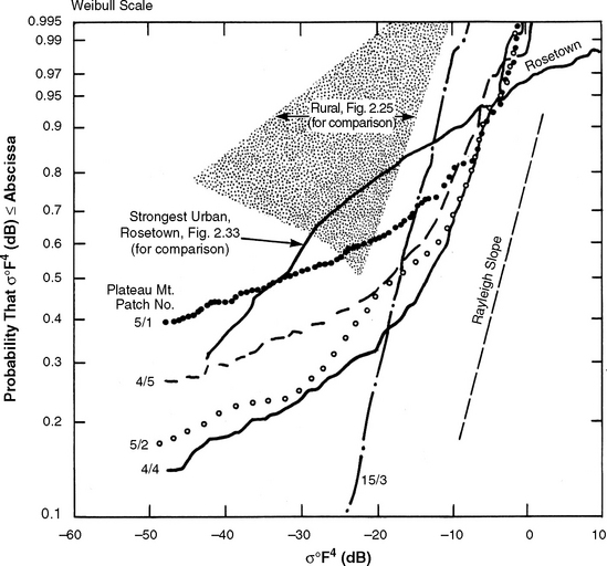
FIGURE 2.32 Ground clutter cumulative amplitude distributions for five patches containing strong clutter from the Rocky Mts. Phase Zero X-band data, Plateau Mt. site, 12-km maximum range experiment, 75-m range resolution, horizontal polarization. See Table 2.6.
First consider patches 4/4, 4/5, 5/1, and 5/2. These four mountain patches represent very strong ground clutter. In terms of mean clutter strength, the strongest patch measured at Plateau Mountain was patch 4/4, at −9.6 dB, approximately 10 dB stronger than the strongest mean clutter from general rural terrain in Table 2.4. In perusing Table 2.6, it is seen that all four of these patches are of steep barren mountain peaks with various incidences of trees on their lower slopes and observed at various depression angles. Mean clutter strengths from these four patches range from −9.6 to −10.8 dB. Taken together, these four patches may be thought of as representing a worst-case (i.e., strongest clutter) for rural terrain.
Altogether at Plateau Mountain there were 43 patches carrying the primary landform classification of “steep.” The average strength of these patches was −21.2 dB. Their average depression angle was +2.7°. The basic Phase Zero clutter modeling information of Table 2.4 predicts mean clutter strength ![]() of −24 or −25 dB for depression angle of 2.7° in high-relief terrain. Of course steep terrain is the extreme case of high-relief. A 3-dB increase in this predicted value of −24 or −25 dB comes very close to the average Plateau Mountain mean strength.
of −24 or −25 dB for depression angle of 2.7° in high-relief terrain. Of course steep terrain is the extreme case of high-relief. A 3-dB increase in this predicted value of −24 or −25 dB comes very close to the average Plateau Mountain mean strength.
Waterton. The other Rocky Mountain site was at Waterton, Alberta. At Waterton the radar was set up on the high prairie in southern Alberta just a few kilometers east of steep mountain terrain. The area around Waterton is characterized by an abrupt transition from prairie to mountains without an intermediate forested foothills region. From the Waterton site, the first range of mountains screened from view other peaks at longer ranges. As a result, only four patches carrying primary landform classification of steep existed at Waterton. Their average strength is −22.0 dB. The average depression angle to these four Waterton patches was −2.8° (i.e., the radar looked up to this steep terrain).
If more precise patch specification could completely avoid all shadowed cells in high-relief terrain, the worst-case clutter strengths that an analyst should assign to mountain terrain would be the “shadowless” mean strengths given in the third column of Table 2.6. The shadowless mean clutter strength is computed as the mean strength from the subset of cells within the patch above radar noise level. It is seen that avoidance of shadowing raises mean strengths by less than 1 or 2 dB for the patches shown in Table 2.6. Use of shadowless statistics must be approached cautiously since they are dependent on the particular sensitivity of the measurement radar.
Bi-Modal Distributions. The clutter amplitude distributions from the four Plateau Mountain patches, patches 4/4, 4/5, 5/1, and 5/2, in Figure 2.32 are bi-modal, meaning that each distribution is widely spread out over relatively weaker clutter strengths, but is much tighter over the strongest clutter strengths. In the cumulative plots of Figure 2.32, each of these four distributions consists of two parts, a shallowly sloped part to the left and a steeply sloped part to the right. The reasons for this bi-modality are as follows. Strong returns from relatively uniform rock faces oriented toward the radar are close to Rayleigh distributed. However, many other possibilities exist for the physical contents of visible resolution cells in mountain terrain, accounting for a large number of returns of widely spread out strength, all non-shadowed and well above radar noise level. These returns from physically complex cells account for the shallow parts of the distributions to the left in Figure 2.32.
Physically complex high-relief cells cannot easily be distinguished a priori from uniformly steep high-relief cells. The interpretation of high-relief bi-modal distributions was validated at one site, Blue Knob, Pennsylvania. At Blue Knob, a steep linear ridge existed across the field-of-view from the site at ∼10-km range. An original patch was specified in the region where the line-of-sight of the radar was normal to the line of the ridge and to the contour lines rising up the ridge. The bi-modal amplitude distribution from this original patch specified on the steep side of the ridge at Blue Knob was separated under smaller, more precise, multiple patch specification into a Rayleigh distribution from a central area of uniform steep planar surface, and several highly spread out distributions from more complex surrounding areas on the side of the ridge.
Consider next the distribution for patch 15/3 in Figure 2.32. Patch 15/3 also has a small left-side shallow portion in its distribution, but it appears at cumulative probability < 0.1. Table 2.6 indicates that patch 15/3 is a steep forested patch rather than a steep barren patch, and that it was observed at a relatively high depression angle of 2.2 degrees. The mean strength of the clutter in patch 15/3 is −16.2 dB. The distribution for patch 15/3 in Figure 2.32 is seen to have a slope very close to the Rayleigh slope. Other indications that patch 15/3 provides close to Rayleigh statistics are that it has the following statistical attributes: ratio of standard deviation-to-mean = 0.15 dB; ratio of mean-to-median = 0.85 dB; ratio of 90 percentile-to-median = 4 dB; ratio of 99 percentile-to-median = 8 dB. Corresponding Rayleigh values are, respectively: 0 dB, 1.6 dB, 5.2 dB, and 8.2 dB.
Most high-relief patches have bi-modal amplitude distributions like patches 4/4, 4/5, 5/l, and 5/2 in Figure 2.32. As a result, the high-relief cumulative ensemble clutter amplitude distributions in the basic clutter modeling information of Figure 2.25 are also bi-modal. The high-relief ensemble distributions of Figure 2.25 only show the right-side steep part of each distribution and are truncated at the left, at the point of onset of the left-side shallow part of the distribution. In Table 2.4, the Weibull distributions approximating the right-side steep parts of the distributions in Figure 2.25 closely match the measured ensemble mean strengths inclusive of their shallow-sloped parts, indicating that mean clutter strength in high-relief terrain is controlled by the right-side steep parts of the amplitude distributions.
Phenomenology. The distinction between low- and high-relief terrain in low-angle clutter is not an arbitrary separation by terrain roughness and steepness as first encountered in Figure 2.23, but more basically relates to shadowing. Low-relief terrain is characterized by large nearly-level regions of general geometric visibility, as predicted by DTED, in which cells containing discrete vertical sources causing strong returns are interspersed with weak cells—either microshadowed, or visible but discrete-free (e.g., see Figure 4.17 and its discussion). In such circumstances, it is not practicable to adjust patch boundaries to avoid interspersed geometrically microshadowed cells and to predict only individual discretes. High-relief terrain is characterized by highly-sloped regions of general geometric visibility in which the majority of cells return discernible clutter. In high-relief terrain, the distinction between cells with and without discretes is less apparent, and it is possible to set patch boundaries so as to contain only visible cells. The differences between these two kinds of terrain are those separating the low-angle specular phenomenon traditionally associated with ground-based radar and the high-angle diffuse phenomenon traditionally associated with airborne radar. Transition from the low-angle to the high-angle regime occurs gradually with increasing depression angle, as illustrated by the data in Figure 2.25 and Table 2.4.
2.4.2.2 URBAN CLUTTER
The basic Phase Zero clutter modeling information of Section 2.4.1 includes general clutter amplitude distributions for urban terrain. Besides such general information, an analyst may wish to know how severe urban clutter can become in worst-case situations. This section provides information on this subject by showing clutter patch amplitude distributions for several of the strongest urban patches measured by the Phase Zero radar. These strong urban patches are compared with the strong mountain patches discussed in Section 2.4.2.1.
Figure 2.33 shows measured cumulative amplitude distributions for three urban clutter patches. The regime of the general urban ensemble distributions from Figure 2.26 is shown lightly shaded in Figure 2.33 for comparison. Table 2.7 shows terrain descriptions, depression angles, and mean clutter strengths for these three patches, which constitute backscatter measurements made from the town of Rosetown, Saskatchewan (population 2,500); the city of Lethbridge, Alberta (population 55,000); and the city of Calgary, Alberta (population 600,000), respectively. All three urban areas exist on the relatively low-relief
TABLE 2.7
Descriptions and Statistical Attributes of Three Urban Clutter Patches at X-Band

aCommercial sector of Rosetown.
bIndustrial section, some open development land, TV tower.
cDowntown Calgary, high rise buildings, Bow River and parks near river, railroad, some residential (minor)

FIGURE 2.33 Ground clutter cumulative amplitude distributions for three patches containing strong urban clutter. Phase Zero X-band data, 75-m range resolution, horizontal polarization, 12-km maximum range experiment. See Table 2.7.
Canadian prairies. In each case, the patch was selected to include only relatively high commercial buildings within the urban complex in contrast to lower outlying residential areas. Differences in clutter strength between commercial and residential urban clutter are discussed subsequently.
Although the data in Figure 2.33 are from three commercial patches, their physical differences are great. Rosetown is a small prairie town providing services to the local agricultural community. Its commercial sector is physically very small but includes grain elevators illuminated at low depression angle. The mean clutter strength of −4.6 dB for the Rosetown patch is the single strongest mean clutter strength that exists within the database of 2,177 Phase Zero patch measurements. However, this Rosetown patch is not particularly exceptional—there are many other relatively small, relatively strong clutter patches from small towns.
It may be preferable to base the worst-case urban clutter strength estimate on larger urban patches than Rosetown, allowing for much more extensive statistical averaging to take place within the distributions. Lethbridge is a moderate-sized regional city in southern Alberta. The industrial area constituting its urban clutter patch is approximately ten times larger than Rosetown but, as was the Rosetown patch, is illuminated at quite low depression angle. Notwithstanding the substantial physical differences in these two patches, their clutter amplitude distributions and mean clutter strengths are very similar. The Calgary patch in Figure 2.33 is approximately twice as large as the Lethbridge patch. Calgary is a major city, and the Calgary patch was selected to include, for the most part, just the high-rise central urban core. Thus the Calgary patch is quite different, physically, from both the Lethbridge and the Rosetown patches. At Calgary, the radar position was on a hill in the outskirts of the city, 490 ft higher than the average terrain height at the city center. Thus the depression angle at which the radar viewed the ground at the city center was substantial, 1.2°, although the highest buildings in the city core were more than 500 ft high. The hilltop location may have resulted in less multipath augmentation and in many surfaces being illuminated at more oblique angle than the near-grazing-incidence illumination at Rosetown and Lethbridge and may be the cause of the somewhat weaker mean clutter strength for Calgary (in Table 2.7) compared with Rosetown and Lethbridge.
Taken together, these three distributions provide a reasonable indication of how strong X-band urban clutter can become. Compared with the general urban distributions of Table 2.4, the data in Table 2.7 indicate that worst-case urban clutter can be 10 dB stronger in mean strength than more general urban levels. This is approximately the same conclusion reached about severe mountain clutter compared with more general high-relief clutter. In terms of mean clutter strength, severe urban clutter can be 5 dB stronger than severe mountain clutter. The Rosetown urban clutter amplitude distribution is included in Figure 2.32 to compare with mountain distributions.
Residential vs Commercial. In considering urban clutter, attention has been restricted to relatively strong urban clutter from commercial sectors. Considered now are the differences in urban clutter strength between residential sectors (expected to be weaker) and commercial sectors (expected to be stronger). Table 2.1 indicates that within the general land cover class of urban, the more specific subclasses of residential and commercial are employed. All the measured clutter amplitude distributions from patches classified by land cover as residential were combined into one ensemble amplitude distribution, and all measured distributions from patches classified by land cover as commercial were combined into another ensemble amplitude distribution. These two clutter amplitude distributions for urban terrain of residential and commercial character, respectively, are shown in Figure 2.34. The regime of the rural amplitude distributions of the basic Phase Zero model is also shown lightly shaded in Figure 2.34 for comparison. Statistical attributes for the residential and commercial ensemble distributions are shown in Table 2.8. These two distributions are quite similar in shape but are horizontally displaced from one another, indicating that clutter from commercial urban sectors is several dB stronger than clutter from residential urban sectors at most percentile levels. In terms of mean clutter strength, Table 2.8 indicates that clutter from commercial sectors is 3.4 dB stronger than clutter from residential sectors. This is regarded as a general result based on measurements from many clutter patches.
TABLE 2.8
Statistical Attributes of Urban Residential and Commercial Ground Clutter Amplitude Distributions*

*Phase Zero X-band data, 75 m range res., hor. pol., 2 to 12 km range. Also see Figure 2.34.

FIGURE 2.34 Comparison of cumulative ground clutter amplitude distributions for urban terrain of residential character and urban terrain of commercial character. Phase Zero X-band data, 75-m range resolution, horizontal polarization, 2- to 12-km range, 113 patches, 33 sites. See also Table 2.8.
2.4.2.3 WETLAND CLUTTER
Figure 2.35 shows cumulative expected value distributions of mean clutter strength from measured Phase Zero patches for four distinctive terrain types—wetland, rural/low-relief, mountains, and urban. The data of Figure 2.35 strongly reinforce the earlier finding that mountain clutter and urban clutter are significantly stronger than most other clutter (i.e., rural/low-relief clutter). At the median position in Figure 2.35, mountain clutter and urban clutter are both about 10 dB stronger in clutter patch mean strength than rural/low-relief clutter. The distribution of mean clutter strength from wetland patches is included in Figure 2.35 with the expectation that wetland might be a terrain type for which clutter might be significantly weaker than most other clutter. Indeed, Figure 2.35 shows that, at the median level, wetland clutter patches are about 5 dB weaker in mean clutter strength than rural/low-relief patches.

FIGURE 2.35 Cumulative distributions of mean ground clutter strength for four distinctive terrain types. Phase Zero X-band data, 75-m range resolution, horizontal polarization, 2- to 12-km range, 1,796 patches, 96 sites. Each curve shows the cumulative distribution of mean clutter strengths from all patches of a given terrain type, one value of mean strength per patch.
Patches of trees often occur on wetland terrain—in thinking about backscatter from general wetland, it is necessary to think as much in terms of clumps of trees and tree lines as in terms of level reed- or sedge-covered marshland or open water conditions. Thus Table 2.1 separates wetland into forested wetland (class 61) and non-forested wetland (class 62) in land cover classification. About half of Phase Zero wetland patches are mixtures of various proportions of forested and non-forested wetland.
All of the Phase Zero wetland clutter patch amplitude distributions were combined into ensemble amplitude distributions in four regimes of depression angle, as shown in Figure 2.36. The regime of the rural amplitude distributions of the basic Phase Zero clutter modeling information is shown lightly shaded in Figure 2.36 for comparison. Statistical attributes for these four wetland ensemble distributions are shown in Table 2.9. These four wetland ensemble distributions are now compared with the rural/low-relief distributions of the basic Phase Zero model (see Figure 2.25 and Table 2.4) at similar depression angles. There is considerable overlap of the wetland ensemble distributions with the rural/low-relief ensemble distributions, compared with the separation of the patch mean clutter strengths of these terrain types in Figure 2.35. In Figure 2.36, the wetland ensemble distributions only separate out as being substantially weaker than the rural/low-relief ensemble distributions at the higher percentile levels—it is the higher percentile levels that control the mean. Comparing ensemble mean clutter strengths (Tables 2.4 and 2.9), rural/low-relief terrain is about 5 dB stronger than wetland in the first three depression angle regimes; in the fourth depression angle regime, 0.75° to 1°, the ensemble mean clutter strength from wetland terrain is approximately equal to that from rural/low-relief terrain.
TABLE 2.9
Statistical Attributes of Wetland Ground Clutter Amplitude Distributions, by Depression Angle*

*Phase Zero X-band data, 75 m range res., hor. pol., 2 to 12 km range. Also see Figure 2.36.
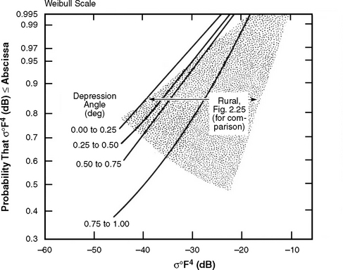
FIGURE 2.36 Cumulative ground clutter amplitude distributions by depression angle for wetland terrain. Phase Zero X-band data, 75-m range resolution, horizontal polarization, 2- to 12-km range, 75 patches, 16 sites. See also Table 2.9.
In comparing the data of Figures 2.25 and 2.36, it is seen that the spreads in the wetland ensemble distributions are much less than those in rural/low-relief ensemble distributions at corresponding depression angles (significantly lower values of aw in wetland). Less spread in clutter amplitude statistics from wetland terrain indicates that wetland is more homogeneous than general rural/low-relief terrain. This is partly due to the fact that wetland is predominantly level, and also partly due to less heterogeneity of land cover in wetland. Because of the general overlap of wetland ensemble amplitude distributions with the corresponding rural/low-relief distributions, they were not separated out as a specific weak-clutter terrain category in the basic Phase Zero clutter modeling information in Section 2.4.1.
2.4.2.4 LEVEL TERRAIN
Level terrain is a canonically simple landform in which only variation in land cover and not variations in surface topology exist to introduce spread in clutter statistics. Thus level terrain provides the opportunity to isolate and understand better the parametric dependencies generally at work in low-angle clutter in which generality can be reached with fewer measurement samples. Twenty-six percent of Phase Zero patches have primary landform classification of level. In what follows, ensemble clutter amplitude distributions for level terrain formed from these level patches are shown for two quite different commonly occurring land cover classes, forest and agricultural, each as a function of depression angle.
Level Forest. All of the Phase Zero clutter measurements from patches of level forest were combined into ensemble amplitude distributions in three regimes of depression angle. The results are shown in Figure 2.37. Statistical attributes for these three level forest ensemble distributions are shown in Table 2.10. The regime of the rural ensemble distributions from Figure 2.25 is shown lightly shaded in Figure 2.37 for comparison.
TABLE 2.10
Statistical Attributes of Ground Clutter Amplitude Distributions for Level Forested Terrain, by Depression Angle*
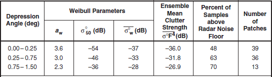
*Phase Zero X-band data, 75 m range res., hor. pol., 2 to 12 km range. Also see Figure 2.37.
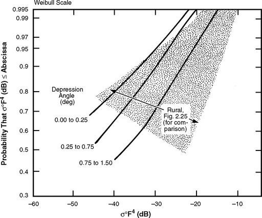
FIGURE 2.37 Cumulative ground clutter amplitude distributions by depression angle for level forested terrain. Phase Zero X-band data, 75-m range resolution, horizontal polarization, 2- to 12-km range, 88 patches. See also Table 2.10.
In the data of Figure 2.37 and Table 2.10, a strong trend with depression angle is observed—with increasing depression angle, spreads in clutter amplitude statistics from level forest rapidly decrease and mean strengths rapidly increase. Compared with clutter amplitude statistics from rural/low-relief terrain at similar depression angles, clutter statistics from level forested terrain have significantly less spread (i.e., much smaller values of aw). This results from the fact that level forested terrain represents a much more homogeneous backscattering medium than rural/low-relief terrain in general, in spite of the fact that, within level forest patches, there exists considerable heterogeneity introduced by higher-order classifiers. For example, 71% of level forested patches carry some category of open terrain (agriculture, rangeland, etc.) as secondary land cover classification.
Level Farmland. Ensemble amplitude distributions in four regimes of depression angle for level agricultural terrain are shown in Figure 2.38. Statistical attributes of these distributions are shown in Table 2.11. The regime of the rural ensemble distributions from Figure 2.25 is shown lightly shaded in Figure 2.38 for comparison. As with level forest, these level agricultural distributions show a strong dependence on depression angle. In other aspects, however, these level agricultural distributions are very different from level forest. The level agricultural distributions show a strong tendency to merge at the higher cumulative probability levels shown (around cumulative probability = 0.97), whereas at such levels the level forest distributions stay well separated. This indicates a dominating influence from discrete clutter sources at these probability levels on level agricultural terrain, from which backscatter would be expected to be less sensitive to depression angle. The spreads in the level agricultural distributions are extreme (much larger values of aw) not only compared with level forest, but also, at very low depression angles (0° to 0.5°), with rural/low-relief terrain in general.
TABLE 2.11
Statistical Attributes of Ground Clutter Amplitude Distributions for Level Agricultural Terrain, by Depression Angle*
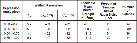
*Phase Zero X-band data, 75 m range res., hor. pol., 2 to 12 km range. Also see Figure 2.38.
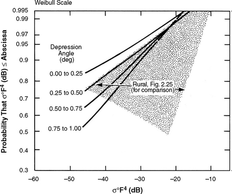
FIGURE 2.38 Cumulative ground clutter amplitude distributions by depression angle for level agricultural terrain. Phase Zero X-band data, 75-m range resolution, horizontal polarization, 2- to 12-km range, 245 patches. See also Table 2.11.
At higher angles (0.75° to 1°), the spread in the level agricultural distribution becomes equal to that of the rural/low-relief distribution. Mean clutter strengths in level agricultural terrain show very little variation with depression angle (although median strengths rise quickly as the spread decreases with increasing depression angle), in contrast to the significantly increasing mean strength with depression angle of level forest. Of the level agricultural patches, 34% carry secondary land cover classification of forest. That is, similarly to level forest containing openings of non-forested terrain, so also does open level agricultural terrain contain patches of trees. Level agricultural terrain is highly heterogeneous because of strong localized discrete scattering sources (including patches of trees) existing in a weakly backscattering medium (the field surfaces themselves).
Comparison with Wetland. Next the characteristics of wetland clutter (Figure 2.36, Table 2.9) are compared with those of level forest (Figure 2.37, Table 2.10). The wetland clutter patches were almost all level. Considered simplistically, both level forest and level wetland might be considered to constitute level vegetative backscattering mediums relatively free of discrete scattering objects. Hence level forest and level wetland might be expected to backscatter relatively similarly, with perhaps wetland causing somewhat weaker clutter because of a possibly enhanced tendency for forward scatter as a result of increased reflection coefficient. Consider next some of the complicating characteristics of real forest and wetland that have been previously discussed. It was indicated in previous discussions of terrain heterogeneity that the majority of wetland patches contained clumps of trees, and that many forested patches contained open areas of, for example, farmland or other open land cover types brought in through second- and third-order classifiers. Thus, from this point of view also, the backscattering characteristics of wetland and level forest might still be expected to be similar.
It turns out that the clutter characteristics of wetland and level forest are, indeed, surprisingly similar. The distributions of Figure 2.36 and Figure 2.37 almost exactly overlay one another in similar regimes of depression angle. (Since the level forest and level wetland depression angle regimes do not exactly coincide, some minor angular interpolation is required to see the match.) This almost exact overlay of the resultant two sets of three curves requires, however, a horizontal displacement of approximately 2 to 3 dB between the two sets of curves, such that the wetland curves are shifted to the right. Thus these data suggest that wetland backscatters very similarly to level forest, except that wetland clutter is about 2 or 3 dB weaker. Thus the initial simplistic speculation that wetland clutter might be like forest clutter, but weaker, is borne out. It is quite remarkable that such similarities should exist between two entirely different data sets, with the approximately 2 or 3 dB offset maintained throughout, depression angle regime by depression angle regime and percentile level by percentile level. The similarity in shapes (Weibull shape parameter aw) and approximately 2 to 3 dB difference in strength between these two data sets is also evident in comparing Tables 2.9 and 2.10.
2.4.2.5 EFFECTS OF TREES
Trees are a dominant component of landscape. In examining any particular low-angle clutter measurement involving trees, the influence of the trees on the backscatter data is often paramount. When large numbers of trees exist as a forest, they cover many other potential sources of clutter on the ground, including discrete cultural objects, so that a relatively homogeneous vegetative medium is presented to the radar. In partially cleared forested regions, the edges of forest can dominate the backscatter. On open agricultural land containing only small incidences of trees, either in isolated occurrence, in shelter belts around farmsteads, in tree lots, or around ponds and along streams, even a small incidence of trees can dominate the landscape in terms of large vertical discrete objects and hence dominate the backscatter.
Because of the importance of trees in low-angle ground clutter, a procedure was implemented within the terrain classification system utilized whereby every clutter patch was classified by percent tree cover. This was done by moving a fine uniform dot pattern over the region of the patch on the air photo and counting the number of dots within the area of the patch containing trees. Clutter statistics were separated into six categories of percent tree cover. For assigning “forest” as the primary land cover classifier of any patch, the percent tree cover within the patch had to be greater than 50%. In what follows, in separating clutter statistics by percent tree cover, all forest patch data were combined to represent greater than 50% tree cover and, for the five remaining categories of percent tree cover less than 50%, patch data were combined from all patches specified to have percent tree cover within each category, irrespective of land cover class.
Ensemble amplitude distributions by percent tree cover η are shown in Figure 2.39 for patches of “level” primary landform classification (similar percent tree cover results were obtained for other landform classes). Statistical attributes of the ensemble distributions of Figure 2.39 are shown in Table 2.12. A significant trend is observed in these distributions, whereby the spread in the distributions as given by the Weibull shape parameter aw strongly decreases with increasing percent tree cover, for percent tree cover between zero and 50%. The “no trees” distribution is a special case. Median clutter strengths gradually increase with increasing percent tree cover, also over the same range for percent tree cover between zero and 50%, but not enough to compensate for the decreasing spread, so to a lesser extent mean clutter strengths tend to decrease with increasing percent tree cover. Spreads in these statistics decrease with increasing percent tree cover between zero and 50% because, with increasing percent tree cover, the sizes of individual stands of trees grow, resulting in fewer isolated trees, tree lines, and edges of stands (with their inherent wide variability in clutter strength) and larger areas covered more or less homogeneously with trees (within each of which the inherent variability in clutter strength is less). For the same reason, the percent of samples above noise level in these ensemble distributions increases with increasing percent tree cover as shown in Table 2.12. In transitioning from the category with percent tree cover between 30% and 50% to the forest category (percent tree cover > 50%), the spread in the amplitude distributions remains about the same (aw = 3.4) but the strengths at most percentile levels increase by about 2 dB.
TABLE 2.12
Statistical Attributes of Ground Clutter Amplitude Distributions by Percent Tree Cover on Level Terrain*

*Phase Zero X-band data, 75 m range res., hor. pol., 2 to 12 km range. Also see Figure 2.39.
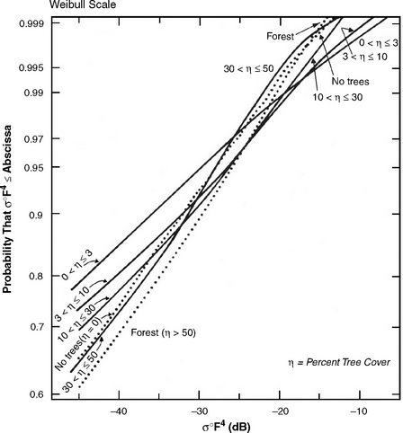
FIGURE 2.39 Ground clutter amplitude statistics by percent tree cover η on level terrain. Phase Zero X-band data, 75-m range resolution, horizontal polarization, 2- to 12-km maximum range, 530 clutter patches. See also Table 2.12.
The “no tree” distribution is a special case, standing outside the general trend of variation in the other distributions with percent tree cover. Simplistically interpreted, “no trees” means, to some extent, “no discretes” (or at least a de-emphasis of discretes). That is, treeless terrain brings out more of the characteristics of area-extensive backscatter from a continuous medium. Forest terrain also begins to show more of the characteristics of a continuous medium, with a de-emphasis on discretes. Hence, simplistically, treeless terrain might be expected to backscatter somewhat like forested terrain. In fact, in Figure 2.39, the “no trees” distribution has abruptly departed from the general trend of increasing spread aw with decreasing percent tree cover and has suddenly assumed much reduced spread characteristics nearly identical to the forest distribution at the other extreme of percent tree cover. In terms of strength, the “no trees” distribution is 2 or 3 dB weaker than the forest distribution.
The data of Figure 2.39 and Table 2.12 clearly show a considerable difference in low-angle clutter characteristics between terrain with absolutely no trees and terrain with “few trees” (where “few” means tree cover between zero and three percent). This emphasizes the importance of isolated trees as the dominant type of discrete clutter source causing the wide spreads seen in low-angle clutter from agricultural land and other open terrain types.
2.4.2.6 NEGATIVE DEPRESSION ANGLE
A small portion of the Phase Zero clutter measurement sites are of negative effective site height. This is the result of terrain features in some directions rising abruptly to elevations higher than the site elevation. Terrain higher than the antenna is observed by the radar at negative depression angle. Ten percent of the 2,177 Phase Zero clutter patches were observed at negative depression angle. To see terrain at negative depression angle from antennas of positive mast height implies a positive terrain slope greater than the absolute value of the particular depression angle involved. Indeed, the terrain occurring above a radar position was often observed to be inaccessibly rough and steep—otherwise, the radar would have been sited at the higher position.
Patches observed at negative depression angle are now separated into three regions of negative depression angle, namely, 0° to −0.25°, −0.25° to −0.75°, and −0.75° to −1.75°, irrespective of terrain type. The clutter data from each of these three sets of patches are combined into an ensemble amplitude distribution. The resultant cumulative ensemble amplitude distributions for three regimes of negative depression angle are shown in Figure 2.40. Statistical attributes for these ensembles are given in Table 2.13. The regime of the rural terrain distributions of Figure 2.25 is shown lightly shaded in Figure 2.40 for comparison.
TABLE 2.13
Statistical Attributes of Ground Clutter Amplitude Distributions in Three Regimes of Negative Depression Angle*

*Phase Zero X-band data, 75 m range res., hor. pol., 2 to 12 km range. See also Figure 2.40.
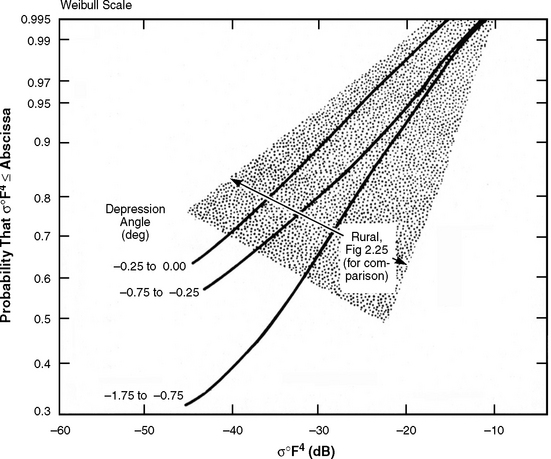
FIGURE 2.40 Cumulative ground clutter amplitude distributions in three regimes of negative depression angle. Phase Zero X-band data, 75-m range resolution, horizontal polarization, 2- to 12-km range, 194 patches. See also Table 2.13.
First, consider the data in the 0° to −0.25° regime. The clutter data within this low negative depression angle regime are dominated by terrain in the undulating and inclined classes presenting slight positive slopes that are visible. In contrast, the clutter data at low positive depression angle from 0° to +0.25° in Figure 2.25 and Table 2.4 are much more influenced by level terrain. As a result, the 0° to −0.25° amplitude distribution is about 2 dB stronger in mean strength than the 0° to +0.25° amplitude distribution and is of less significantly spread (aw = 3.9 compared with 4.8).
Next, consider the data in the −0.25° to −0.75° depression angle regime. Within this regime, many of the patches have moderately steep or steep landform components. As a result, the clutter amplitude distribution in the −0.25° to −0.75° depression angle regime is about 5 dB stronger in mean strength than the corresponding distribution at positive depression angle. In terms of spread, however, the shape parameter aw at −0.25° to −0.75° is very similar to that for terrain at corresponding positive depression angles.
For depression angles from −0.75° to −1.75°, these trends continue but with increasing domination by high-relief terrain. The clutter amplitude distribution in this regime is similar to corresponding distributions in the 0° to 1° and 1° to 2° regimes in high-relief terrain. In moving from the −0.25° to −0.75° depression angle regime to the −0.75° to −1.75° regime, the increased incidence of steep terrain has increased mean strength very little but has substantially reduced the spread aw.
Thus, it is evident that clutter amplitude statistics at negative depression angles are, on the whole, relatively dissimilar to amplitude statistics at corresponding positive depression angles. At low negative angles (i.e., 0° to −0.25°), strengths are somewhat higher and spreads are somewhat lower than corresponding positive angles because the generally low-relief terrain surfaces under observation at low negative angles have to be slightly more inclined towards the radar to be seen. At slightly higher negative angles (i.e., above −0.25°), the only terrain usually seen is for the most part quite rough and steep, with attendant increases in clutter strength. Once the terrain is high enough and steep enough to be observed at significant negative depression angles (i.e., depression angle < −0.25°), further increases in negative depression angle (i.e., depression angle < −0.75°) do not significantly increase mean clutter strengths but do continue to significantly decrease clutter spreads.
2.4.3 COMBINING STRATEGIES
2.4.3.1 ENSEMBLE DISTRIBUTIONS VS EXPECTED VALUES
Throughout Section 2.4, general understandings and descriptions of the low-angle clutter phenomenon have been sought for the most part by combining measurement data from many individual, like-classified, clutter patches into ensemble amplitude distributions generally representative of that class. In combining clutter data, individual spatial cells or samples can represent the elemental spatial quantity being combined, or clutter macropatches—each patch containing many cells—can represent the elemental quantity.
First consider combination at the cell level. Imagine from a set of like-classified patches, a set of clutter amplitude histograms—one histogram per patch—that all have identical bell shapes but that have widely varying means so that there exists little overlap from histogram to histogram. Aggregation of the data in all of these elemental histograms, cell by cell, into one overall ensemble histogram, yields an ensemble histogram of quite different characteristics from any of the individual histograms. In particular, in these circumstances the ensemble histogram contains much more spread in its data than any of the individual histograms.
The failure of the above set of histograms as a proper ensemble is the failure of the classification system that grouped the patches together in the first place. Now, from a set of like-classified patches, imagine a set of histograms of similar but not identical shape, with similar means and standard deviations, but with each histogram containing different specific higher-order attributes. Combining these histograms cell-by-cell into an ensemble histogram yields a useful general distribution in which individual differences are averaged out. The resultant ensemble distribution is generally representative of any of the individual histograms. This situation is the result of a classification system which successfully finds and groups together patches with similar amplitude statistics in the first place. In the actual world of clutter patches, neither of the above positions is entirely true. The classification system utilized works usefully but not perfectly. As a result, aggregation of amplitude statistics from a set of patches sample by sample at the spatial cell level does provide much useful information, but it also introduces some extra spread into the resultant ensemble distributions.
The above discussion is now quantified around a specific example; namely, the ensemble of rural/low-relief terrain with depression angle from 0.25° to 0.5°. This ensemble contains 448 individual clutter patches giving rise to 448 individual clutter amplitude histograms. For each patch, the mean strength of its histogram is computed, and the distribution of 448 mean strengths is plotted cumulatively in Figure 2.41. Given this set of data, the task of modeling is to select an appropriate general value for representing mean clutter strength in rural/low-relief terrain at depression angles from 0.25° to 0.5°.
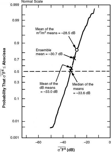
FIGURE 2.41 Cumulative distribution of mean ground clutter strength for rural/low-relief terrain with depression angle from 0.25° to 0.5°. Phase Zero X-band data, 75-m range resolution, horizontal polarization, 2- to 12-km range, 448 patches, 70 sites. The curve shows the distribution of mean strengths, one value of mean strength (Eq. 2.B.8) per patch. See text for definitions of indicated central measures of the distribution.
Observe that the cumulative distribution in Figure 2.41 is quite linear as plotted against the normal probability scale there. To the extent that it is linear, the distribution can be represented by a normal or Gaussian distribution. That is, the distribution of dB values of mean patch clutter strength (each mean computed in units of m2/m2 and subsequently converted to dB, as per Eqs. (2.B.3) and (2.B.8), in Figure 2.41 is closely approximated by a well-behaved normal distribution. This being the case, a reasonable value to select from this distribution as being generally representative of rural/low-relief, 0.25° to 0.5° depression angle, mean patch clutter strength is the median value in the distribution, −33.6 dB. If the distribution were exactly symmetrical, its mean, median, and modal measures of dB values would be identical. The mean value of the dB values of mean clutter strength [calculated similarly to Eq. (2.B.12), although with yi representing mean clutter strength of the i-th patch in dB as computed by Eq. (2.B.8)] in Figure 2.41 is −33.0 dB.
If the distribution of dB values of mean clutter strength in Figure 2.41 is normal, then the distribution of the values of mean clutter strength in units of m2/m2 is lognormal. All of the percentile values in this fundamental m2/m2 distribution simply transform logarithmically to corresponding values in the dB distribution (e.g., the median position in the m2/m2 distribution is also the median position in the dB distribution). But mean and modal values in the m2/m2 distribution are not simply related to corresponding values in the dB distribution, and do not occur at the same percentile positions in the m2/m2 distribution as they do in the dB distribution. The mean value of the m2/m2 values of mean patch clutter strength in the distribution of Figure 2.41 is −28.5 dB, 4.5 dB stronger than the mean value of the dB values of mean patch clutter strength in the same distribution. Note that this value of −28.5 dB occurs at the 82-percentile level in the distribution.
Finally, consider the overall ensemble histogram of individual cell-by-cell spatial samples assembled aggregatively from the 448 patches corresponding to the data of Figure 2.41. The mean value of this ensemble histogram computed in m2/m2 and converted to dB [by Eqs. (2.B.3) and (2.B.8)] is −30.7 dB. This value of −30.7 dB occurs at the 72-percentile level in the distribution. Let this value, −30.7 dB, be called the cell-level ensemble mean. Comparing it to the mean of the m2/m2 means = −28.5 dB, the mean of the dB means = −33.0 dB, and the median of the means = −33.6 dB, the ensemble mean lies between the mean of the m2/m2 means and the mean of the dB means, 1.2 dB below the former and 2.3 dB above the latter. The ensemble mean is not equal to the mean of the m2/m2 means because the clutter patches are not all of equal size; if they were, these two quantities would be identically equal.
At this point in the discussion, three reasonable definitions of mean clutter strength exist to represent a patch of rural/low-relief terrain observed at 0.25° to 0.5° depression angle. There is no single correct definition. The clutter modeler wants to select a reasonable definition appropriate to the application of the model. The modeler wants to look for parametric trends in this defined quantity and wants to stay aware of the extent to which the characteristics of such trends might be dependent on the quantity selected.
There is nothing in Figure 2.41 to discourage use of the ensemble aggregation of cell-level statistics to model clutter. The ensemble mean occupies middle ground between the mean of the dB means and the mean of the m2/m2 means at the 72-percentile level in the distribution. Thus a model based on ensemble aggregations of cell-level statistics is biased somewhat towards more severe clutter leading to conservative estimates of radar capability. This is not necessarily undesirable. In overview, there are many patches with both stronger and weaker clutter strength than the ensemble mean value.
At the beginning of Section 2.4, the question was raised of whether cell values or patch values should be regarded as elemental spatial statistical quantities to be combined in clutter modeling. The data in Figure 2.41 show the combination of all patch mean clutter strengths for a given ensemble of patches. Thus within the distribution of Figure 2.41, the patch is the elemental quantity. The particular statistical attribute of the patch amplitude histogram that is quantified in Figure 2.41 is patch mean strength. Other statistical attributes of patch amplitude may be similarly plotted (see Figure 2.42). The advantage of regarding patches as elemental statistical quantities is that it avoids cell-level aggregation of data from non-similar histograms. However, once the distribution of a particular patch attribute is plotted such as in Figure 2.41, the modeler still has to face up to selecting one value from a range of values.
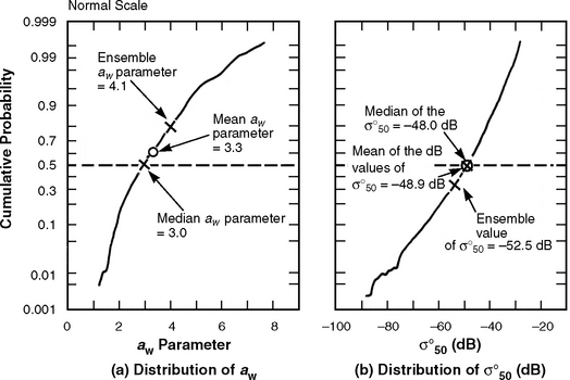
FIGURE 2.42 Cumulative distributions of approximating Weibull coefficients aw and ![]() (dB) for clutter patch amplitude distributions for rural/low-relief terrain with depression angle from 0.25° to 0.5°. Phase Zero X-band data, 75-m range resolution, horizontal polarization, 2- to 12-km range, 448 patches, 70 sites. The curves show distributions of Weibull shape parameter aw and mean clutter strength
(dB) for clutter patch amplitude distributions for rural/low-relief terrain with depression angle from 0.25° to 0.5°. Phase Zero X-band data, 75-m range resolution, horizontal polarization, 2- to 12-km range, 448 patches, 70 sites. The curves show distributions of Weibull shape parameter aw and mean clutter strength ![]() , one value of each per patch.
, one value of each per patch.
In the end, it still is an act of reasoned judgment to select the modeling quantity. If it is argued that a cell-level aggregative approach to ensemble statistics is too demanding of a terrain classification system, it is certainly true that a failed classification system also fails at the patch level. Under a failed system, collections of patch attributes will contain much spread and show no parametric variation. The advantage of forming cell-level aggregative ensemble distributions is that it is a convenient way to show resultant averaged or generalized amplitude distributions. That is, the general histogram is just the sample-by-sample sum of the data in the individual histograms. It is less easy to provide an actual general histogram or cumulative distribution in a patch-oriented approach in which only various attributes of individual patch histograms are collected, as opposed to the histograms themselves.
One thing that can be done in this regard is to approximate the shape of each individual patch amplitude distribution with a Weibull shape parameter aw The distribution of all such values of aw can then be formed for a particular ensemble of patches. Such a result is shown in Figure 2.42(a), for the same rural/low-relief, 0.25° to 0.5° depression angle ensemble for which data are shown in Figure 2.41. Three representative values for aw are also indicated in Figure 2.42(a), the median value of aw equal to 3.0, the mean value of aw equal to 3.3, and the value of approximating shape parameter aw for the cell-level aggregate distribution previously obtained (see Table 2.4) equal to 4.1. This last quantity is denoted as the cell-level ensemble value of aw.
The data shown in Figure 2.42(a) quantify the concern discussed at the beginning of Section 2.4; that cell-level aggregation can cause too much spread in resultant average distributions. The ensemble value of aw is, indeed, greater than the mean or median values of aw in Figure 2.42(a). The ensemble value of aw is at the 80-percentile level in the distribution. Consider that the median level does not necessarily constitute a better modeling value than the 80-percentile level. There are many individual patches with both significantly greater spread and significantly less spread than that specified by the ensemble value of aw in the data of Figure 2.42(a). However, use of the cell-level aggregation does provide a slight bias towards increased spread in clutter amplitude statistics in the modeling information of Chapter 2, as well as increased strength. Again, such a conservative bias from the point-of-view of radar capability is not necessarily undesirable. It does, however, require quantification. In the data of Figure 2.42(a), this bias is not extreme. The bias is most extreme at the lowest depression angles, as in the depression angle regime of 0.25° to 0.5° for which data are shown in Figures 2.41 and 2.42. The bias decreases with increasing depression angle. Comprehensive modeling information of clutter amplitude statistics based on patch-level expected-value characterization is the main approach taken in subsequent chapters in this book. This is a more challenging empirical task than that based on simple cell-level sample-to-sample ensemble aggregation.
Besides the shape parameter aw, a Weibull model requires specification of the ![]() parameter. In approximating the clutter amplitude distribution of each of the 448 rural/low-relief patches observed at 0.25° to 0.5° depression angle with a Weibull distribution, besides collecting all of the patch values of aw as shown in Figure 2.42(a), all of the patch
parameter. In approximating the clutter amplitude distribution of each of the 448 rural/low-relief patches observed at 0.25° to 0.5° depression angle with a Weibull distribution, besides collecting all of the patch values of aw as shown in Figure 2.42(a), all of the patch ![]() (dB) values were also collected as shown in Figure 2.42(b). It is observed that the ensemble value of
(dB) values were also collected as shown in Figure 2.42(b). It is observed that the ensemble value of ![]() is 4.5 dB weaker than the median value. This also reflects the increased spread of cell-level aggregate models compared with aggregates of patch attributes. The increased spread of the cell-level distribution has driven
is 4.5 dB weaker than the median value. This also reflects the increased spread of cell-level aggregate models compared with aggregates of patch attributes. The increased spread of the cell-level distribution has driven ![]() in the approximating Weibull distribution to somewhat lower levels (i.e., 33 percentile) in the distribution of patch-level
in the approximating Weibull distribution to somewhat lower levels (i.e., 33 percentile) in the distribution of patch-level ![]() values. Again, compared to the overall range of this distribution, this value of −52.5 dB appears reasonable for a general model.
values. Again, compared to the overall range of this distribution, this value of −52.5 dB appears reasonable for a general model.
In the end, the relative goodness or badness of the cell-level ensemble aggregate approach is the fidelity with which the ensemble distribution represents a typical patch distribution. As indicated by the comparisons with constituent patch data shown in Figures 2.41 and 2.42, the rural/low-relief, 0.25° to 0.5° depression angle, ensemble aggregate distribution on the whole satisfactorily represents a clutter amplitude distribution from a typical clutter patch.
2.4.3.2 STATISTICAL CONVERGENCE
Consideration now is given to whether a given ensemble of like-classified patches contains enough patches to provide generality. A simple empirical test for whether a trial set of patches is sufficient to provide converged results18 characteristic of the general set is to simply randomly partition the trial set any number of ways into two equal and independent subsets, each containing half as many patches as the original set, and to subsequently determine if the results obtained from the subsets agree with those of the original set [15]. Continuing with the rural/low-relief, 0.25° to 0.5° depression angle ensemble of 448 patches selected for previous discussion in Section 2.4.3.1, these patches are now randomly divided into two subsets, each containing 224 patches. This is done in three different ways. For each of these six subsets, the cell-level ensemble clutter amplitude distribution is formed and plotted cumulatively in Figure 2.43.

FIGURE 2.43 Three halvings of the 0.25° to 0.5° depression angle, rural/low-relief ensemble clutter amplitude distribution. Phase Zero X-band data, 75-m range resolution, horizontal polarization, 2- to 12-km range. Full ensemble mean clutter strength = −30.72 dB.
It is apparent in Figure 2.43 that, within each partition generating two independent subsets, each independent pair of distributions are closely converged to one another. On the basis of these results, it is expected that, if a new clutter measurement program were to be initiated, in which clutter was measured from 448 newly selected patches of similar classification, the new measurements would lead to a new cell-level ensemble clutter amplitude distribution well within the interval of uncertainty indicated in Figure 2.43.
2.4.4 DEPRESSION ANGLE CHARACTERISTICS
2.4.4.1 GENERAL CHARACTERISTICS
A traditional approach to ground clutter modeling is to specify clutter strength as a simple characteristic of illumination angle. Following this approach, Figure 2.44 shows generalized mean and median clutter strengths as a function of depression angle, inclusive of all terrain types. The results of Figure 2.44 are based on Phase Zero measurements of 1,926 macropatches from 86 sites. Figures 2.45 and 2.46 show the ratio of standard deviation-to-mean vs depression angle and the incidence of occurrence of microshadowing within clutter patches vs depression angle, respectively, for the same set of Phase Zero data upon which the results in Figure 2.44 are based. At very low angles, clutter is caused to a very great extent by discrete sources distributed over a weakly backscattering surface. Hence, at very low angles, less than half (38%) of cells within visible patches contain clutter discernible to the Phase Zero radar. As angle rises through the low-angle regime (depression angle < 2°), the percent of cells containing discernible clutter rises very quickly as the shadowed terrain between discrete sources rapidly comes into view. As a result, the median clutter strength, which was driven down by the large number of shadowed cells at very low angles, also rises relatively quickly with increasing depression angle. Median clutter strength does not rise quite as abruptly as the shadowing function, because even when terrain comes into visibility at very low angle, the area-extensive backscatter from the terrain surfaces themselves, as opposed to the discrete objects on them, is very weak.
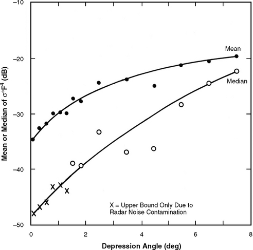
FIGURE 2.44 General variation of ground clutter strength with depression angle. Phase Zero X-band data, 75-m range resolution, horizontal polarization, 2- to 12-km range. All terrain types, 1,926 patches from 86 sites. Data shown are expected values, see text.
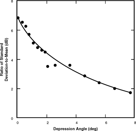
FIGURE 2.45 General dependence of ratio of standard deviation-to-mean in ground clutter spatial amplitude statistics on depression angle. Phase Zero X-band data, 75-m range resolution, horizontal polarization, 2- to 12-km range. All terrain types, 1,926 patches from 86 sites. Data shown are expected values, see text.
With increasing angle, however, as the shadowing function levels off, the median clutter strength continues to rise as area-extensive backscatter rises with increasing angle. Mean clutter strengths rise less rapidly than median clutter strengths, because the means are dominated more by the discrete vertical sources and less by the statistics of shadowing. The ratio of mean-to-median in Figure 2.44 and the ratio of standard deviation-to-mean in Figure 2.45, which are measures of spread in clutter amplitude distributions, both decrease strongly with increasing angle as the shadowed and weak samples at the low end of the distributions rise towards the stronger values that are dominating the mean. In the high angle limit of 8° for the data in Figures 2.44 and 2.45, both these measures of spread begin to approach their limiting values associated with Rayleigh statistics. This reflects the relatively low incidence of microshadowing (14%) and relatively full illumination prevailing at high angles.
In modeling ground clutter at the high depression angles associated with airborne platforms, clutter strength is often approximated as being directly dependent on the sine of the depression angle. Such a model is referred to as “constant γ,” where σ° = γ sin α (see Sections 1.2.5 and 2.3.4.2). Typical decibel values of γ (i.e., 10 log10γ) in use for rural terrain are −10 and −15 dB [5, 10, 16]. The mean clutter strength curve above 1° in Figure 2.44 is very accurately represented by σ° = γ (sin α)1.2 with a decibel value of γ equal to −8.9 dB. Note that the exponent to which sin α is raised in this latter expression is 1.2; that is, the sin α dependence of the Phase Zero data in Figure 2.44 above 1° (457 macropatches) is somewhat stronger than the linear dependence often assumed [5, 10, 16]. Fitting the constant-γ model with linear sin α dependence to the mean clutter strength data above 1° in Figure 2.44 leads to a decibel value of γ of approximately −11 dB, although doing so results in a poorer fit to the data. A summary of simple semi-empirical clutter models such as the constant-γ model and its variations that have been utilized historically to fit various experimental data sets is provided in Ruck [17].
At lower angles, however, where most land clutter occurs in surface-sited radar, mean clutter strength is much stronger than is predicted by the sine of the depression angle dependency, the latter becoming vanishingly small as depression angle approaches zero. Strong mean clutter at low angles is the consequence of domination of the low-angle phenomenon by discrete clutter sources. There has been occasional speculation in the clutter literature as to whether clutter strengths might “come back up” at very low angles because of possible specular incidence on discretes. The data of Figure 2.44 indicate that, although mean clutter strength remains relatively high at low angles, its general characteristic is to always decrease with decreasing angle, with no reversal occurring in this characteristic at very low angle.
Mean clutter strength is observed to vary over a range of 15 dB with depression angle in Figure 2.44, from −34.2 dB at grazing incidence in the 0° to 0.25° depression angle regime to −19.3 dB in the 7° to 8° regime. This mean strength variation of 15 dB with depression angle is the most significant general parametric variation observed of any single parameter in the Phase Zero X-band data. The effect of higher average terrain slopes at higher depression angles is implicit in this dependence. The dependence may be summarized by saying that it is depression angle as it influences shadowing on a sea of discretes that most directly affects strength in low-angle ground clutter.
Most of the measured Phase Zero data occur at low depression angle. For example, 95% of Phase Zero patches were observed at depression angles of < 2.6°. Thus, in Figures 2.44, 2.45, and 2.46, in the 0° to 0.25° depression angle regime there are 456 patches contributing, but in the 7° to 8° depression angle regime there are only 3 patches contributing. The major information content in these figures is at the low angles—available data are included at higher angles to show a more complete depression angle characteristic. The data in Figures 2.44 and 2.45 are expected-value results. The microshadowing data in Figure 2.46 are ensemble values.
2.4.4.2 FARMLAND VS FOREST
Figure 2.47 shows how the depression angle characteristics of low-angle clutter strongly depend on terrain type. In this figure, ![]() and aw are shown as a function of depression angle for four rural terrain types. First, if rural terrain is separated into low relief (terrain slopes < 2°) and high relief (terrain slopes > 2°), in both categories of relief
and aw are shown as a function of depression angle for four rural terrain types. First, if rural terrain is separated into low relief (terrain slopes < 2°) and high relief (terrain slopes > 2°), in both categories of relief ![]() increases and aw decreases with increasing depression angle; and
increases and aw decreases with increasing depression angle; and ![]() is significantly greater and aw significantly less in high-relief terrain than in low-relief terrain, for a given depression angle. The results of Figure 2.47 may be compared with those of Figure 1.9 in Chapter 1.
is significantly greater and aw significantly less in high-relief terrain than in low-relief terrain, for a given depression angle. The results of Figure 2.47 may be compared with those of Figure 1.9 in Chapter 1.

FIGURE 2.47 X-band ground clutter results for (a) rural/low-relief terrain, (b) rural/high-relief terrain, (c) level farmland, and (d) level forest.
Second, if within general rural/low-relief terrain specific subcategories of level farmland and level forest are separated out, Figure 2.47 shows that with increasing depression angle in level farmland ![]() does not vary at all, but aw rapidly decreases, whereas in level forest
does not vary at all, but aw rapidly decreases, whereas in level forest ![]() gradually increases and aw gradually decreases.
gradually increases and aw gradually decreases.
The reasons for this are as follows. In level farmland dominant clutter sources are large, discrete, vertical objects, which at low depression angles cause the clutter amplitude distributions to have very large spread. As depression angle increases, the weak returns from the intervening terrain between strong discrete sources rapidly increase, causing spreads in amplitude distributions to rapidly decrease, but the strong returns from the discrete objects continue to dominate their mean strengths relatively independent of depression angle. In contrast, level forest is much more a homogenous scattering medium, not dominated by large discrete objects. Nevertheless, at low angles in level forest, there still occurs a large amount (e.g., 50%) of microshadowing. As angle increases, the shadowing gradually decreases. As a result the amplitude distributions gradually tighten up, and their mean strengths—not dominated here by large singular discrete sources—gradually rise.
The depression angle characteristics of Figure 2.47 were obtained from ensemble clutter amplitude distributions previously discussed in Section 2.4—the rural/low-relief and rural/high-relief data come from Section 2.4.1, and the level farmland and forest data come from Section 2.4.2.4.
2.4.4.3 SOME AIRBORNE CLUTTER MEASUREMENTS
As part of the ground clutter studies at Lincoln Laboratory, some airborne ground clutter data were collected with an X-band synthetic-aperture radar (SAR) contemporaneously with the ground-based Phase Zero program. Motivation existed to collect airborne data to validate the presumed better understanding of airborne clutter and to provide some connectivity to ground-based measurements at higher angles. Clutter statistics at the higher angles provided by an airborne platform were expected to be approximately Rayleigh distributed—if so, this would largely confirm that the airborne clutter phenomenon is properly represented in traditional manner as a simple constant-γ angle characteristic.
The SAR was mounted on a Convair 580 aircraft. The SAR operated at both L- and X-bands but only X-band data are discussed in what follows. The resolution of the SAR at X-band was six meters. Calibrated X-band ground clutter measurement data were collected at six measurement sites of various terrain types in western Canada in side-looking ground swath or strip map mode. Depression angle ranged from 4° to 18°. Within each 5 km × 30 km ground swath, many clutter patches of uniform terrain were identified. The terrain within these clutter patches was characterized through use of maps and air photos. For each patch, the clutter distribution was formed and pertinent parameters such as mean, median, and standard deviation were calculated.
Figure 2.48 shows clutter results from many patches selected from all six sites. These results show mean values of clutter strength from each patch as scatter plots vs depression angle, separated in four classes of terrain—agricultural, rangeland, forest, and wetland. Each scatter plot shows wide variability, although suggestions of trends of increasing mean strength with increasing depression angle are evident in each plot. Overall, mean clutter strength in agricultural terrain and forest is stronger, compared to rangeland and wetland where it is weaker. However, as in the Phase Zero low-angle data, wide variability exists within terrain class and little separation exists between classes in these airborne data.

FIGURE 2.48 X-band SAR airborne clutter measurements: clutter strength vs depression angle for four terrain types.
Figure 2.49 focuses on agricultural patches collected at five sites. The top two scatter plots show mean and median clutter strength vs depression angle. The bottom two scatter plots show patch values of standard deviation vs mean and mean vs median. A regression curve is shown through each of the top two scatter plots. These curves indicate that, as expected, both mean and median clutter strengths gradually increase with increasing depression angle. Furthermore, they indicate that the mean strength is slightly stronger than the median. The bottom two plots indicate that the standard deviation is usually very nearly equal to the mean (in Rayleigh statistics, standard deviation = mean), and that the mean is usually 1 or 2 dB stronger than the median (in Rayleigh statistics, mean/median ratio = 1.6 dB). Hence these farmland data strongly suggest near-Rayleigh statistics, based on the first two moments and the median of clutter amplitude distributions measured over many (622) clutter patches.
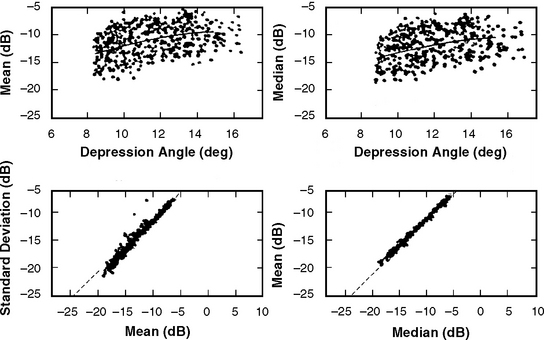
FIGURE 2.49 X-band SAR airborne clutter measurements: clutter patch statistics in agricultural terrain.
Early reduction of the SAR X-band clutter measurement data was based on optical processing in which cumulative distributions of clutter patch amplitude statistics appeared to be lognormal. Subsequent finalized reduction of the SAR clutter measurement data utilized digital processing. Comparison with the digitally processed data revealed that the lognormal distributions of the optically reduced data were caused by an averaging effect in the optical processor due to the finite sample aperture. The digitally processed data, as expected, showed near-Rayleigh distributions, as shown by the results of Figure 2.50 and
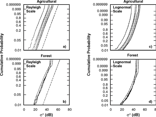
FIGURE 2.50 X-band SAR cumulative clutter distribution for sample patches in agricultural and forest terrain. Rayleigh (a),(b) vs lognormal (c),(d) probability scales.
Table 2.14. Figure 2.50 shows plots of cumulative distributions of amplitude distributions from a number of clutter patches of agricultural terrain—top [(a) and (c)], and forest terrain—bottom [(b) and (d)]; plotted against a Rayleigh probability scale—left [(a) and (b)], and a lognormal probability scale—right [(c) and (d)]. It is evident that all of these measured patch cumulatives without exception are very linear on the Rayleigh scale and are very much upwards curved on the lognormal scale, strongly indicating that all these patch cumulatives are well approximated as Rayleigh distributions. Table 2.14 confirms this finding in terms of mean/median ratio (Rayleigh = 1.6 dB), and sd/mean ratio (Rayleigh = 0 dB). These results indicate that the agricultural data are indeed very nearly Rayleigh; whereas the forest data are on the whole of just slightly more spread than purely Rayleigh.

Thus, with respect to spatial amplitude statistics, these airborne clutter data are indeed of simple behavior and well approximated as tight Rayleigh or quasi-Rayleigh distributions. Next, consider continuity with depression angle between the low-angle Phase Zero data and the higher-angle airborne data. Figure 2.51 shows global characteristics of mean clutter strength vs depression angle as measured across very many rural clutter patches for both ground-based Phase Zero data and the X-band SAR airborne data. Most of the ground-based data are at angles below 2° depression angle; most of the airborne data are at angles above 8°. General continuity of increasing mean clutter strength with increasing angle inclusive of both ground-based and airborne angle regimes and including the more lightly sampled crossover regime is evidenced in the data of Figure 2.51; a single overall characteristic of mean strength vs depression angle closely approximates these data.

Thus ground-based and airborne land clutter, which at first observation appear to be completely different phenomena, can be viewed as a single continuous process connected by depression angle. At low angles clutter distributions are very broad and spread out because of effects of discrete sources and microshadow. With increasing angle, mean clutter strengths rise and spreads diminish. Eventually, at high enough angles, floodlit illumination occurs with no microshadowing and little effect from discretes. The spiky discrete-dominated heterogeneous Weibull process at low angles gradually converts over, with increasing depression angle, to more diffuse clutter and the accompanying homogeneous Rayleigh process that exists in airborne radar.
2.4.5 EFFECT OF RADAR SPATIAL RESOLUTION
Ensemble amplitude distributions were formed from ground clutter measured at each of the three Phase Zero pulse lengths over common spatial regions between 2 and 6 km in range from the radar at 14 sites of various terrain types. The three pulse lengths available were 60 ns, 0.5 μs, and 1.0 μs; corresponding range resolutions were 9, 75, and 150 m. The ratio of standard deviation-to-mean was computed as a measure of spread for each of these three ensemble distributions and plotted vs range resolution in Figure 2.52. The results in Figure 2.52 indicate a strong trend of increasing spread in low-angle clutter amplitude distributions with increasing resolution, or in other words, with decreasing resolution cell size A. In the discrete-dominated, heterogeneous process of low-angle clutter, increasing resolution results in less averaging within cells, more cell-to-cell variability (i.e., more strong cells, more weak cells), and increasing spread in clutter amplitude distributions. A scale showing Weibull shape parameter aw as it varies with ratio of standard deviation-to-mean in Weibull distributions is also shown in Figure 2.52.
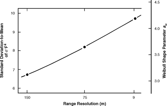
FIGURE 2.52 Spread in clutter amplitude statistics vs resolution. Phase Zero X-band data measured at each of the three Phase Zero pulse lengths over common spatial regions from 2 to 6 km in range at 14 sites of various terrain types.
The characterization of low-angle clutter strength by σ°, an area density function, implies spatial homogeneity of land clutter. If each clutter resolution cell in a spatial field contained a large number of elemental scatterers with no single scatterer dominating, cell-to-cell variations in clutter amplitudes would be Rayleigh distributed. In these circumstances, neither the mean strength of the distribution of clutter amplitudes over the spatial field nor their spread would vary with resolution cell size. However, the conditions for Rayleigh statistics do not apply to low-angle clutter—strong discretes often dominate within low-angle cells. In these circumstances, Phase Zero results indicate that the mean strength over the spatial field or clutter patch is still largely insensitive to the resolution cell area, thus validating the basic characterization of low-angle clutter as properly being a density function σ°. However, as indicated in the results of Figure 2.52, the spreads in low-angle clutter amplitude distributions take on much greater values than Rayleigh (for Rayleigh voltage statistics and hence exponential σ° statistics, aw = 1; ratio of standard deviation-to-mean = 0 dB) and vary strongly with resolution cell size A.
It is fundamentally important to accurately model the wide spreads that occur in low-angle land clutter. These spreads strongly affect radar performance in clutter through target detection and false alarm statistics. The results of Figure 2.52 provide a first indication of the effect of radar resolution cell size on spreads in low-angle clutter and a preliminary means to adjust the Phase Zero modeling information of Chapter 2—heretofore provided as clutter modeling information based on range resolution of 75 m—to apply to other resolutions. In subsequent chapters, the dependence of spread in low-angle clutter spatial amplitude distributions is developed as fundamentally dependent on radar spatial resolution from the outset within the basic parameterization of the modeling information provided.
2.4.6 SEASONAL EFFECTS
Microwave backscatter from terrain depends upon the fine-scale structure of the landscape surfaces being illuminated. Dynamic processes of change associated with season, weather, human activity (i.e., land use), and even plant morphology (i.e., diurnal variability) cause these surfaces to be continuously varying. The effects of such variations on clutter statistics and the extent to which they need to be incorporated in clutter modeling require investigation.
The overall effects of season on land clutter are not obvious. If attention is focused on a single agricultural field, its constitutive characteristics and hence radar backscatter will be considerably different in the summer when it is covered with mature wheat than in the winter after the wheat has been harvested to stubble and the field is covered with snow. However, it has been shown that over large composite landscapes as viewed by ground-based radar, backscatter is often largely caused by macroscopic features of vertical discontinuity (e.g., treelines, woodlots, towns, ridge tops, vertical obstructions along roads and field boundaries, etc.). To the extent that the major physical characteristics of such vertical features do not change substantially with season, it may be that seasonal effects on clutter are not strong.
This latter supposition is supported by the data of Figure 2.53. This figure compares summer and winter Phase Zero clutter measurements at Gull Lake West, Manitoba. The Gull Lake West site (as previously discussed at some length in Section 2.3.3) presented a mixed woodland and farmland scene with many composite features, including a railway, a high voltage power line, rivers and streams, the shoreline of a large lake, and considerable areas of wetland, all over relatively low-relief terrain and viewed from a local site elevation advantage of 100 ft. The winter measurements were performed in February with deep snow cover over the fields, plowed roads with high snowbanks, frozen streams and lake (with piled ice along the shoreline), and with all deciduous trees bare of leaves. The summer measurements were performed in June with crops up, leaves out, and the countryside generally verdant. In comparing summer and winter data for many clutter patches at Gull Lake West, very few significant differences were observed.
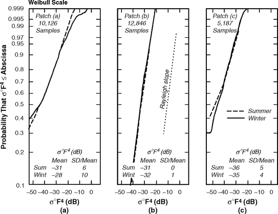
FIGURE 2.53 Seasonal variations in low-angle clutter amplitude statistics for three clutter patches. Phase Zero data, 75-m range resolution. Gull Lake West, Manitoba. (a) Composite cropland/mixed forest, dep. ang. = 0.7°; (b) level uniform forest, dep. ang. = 1.1°; (c) mixed forest/cropland (with river), dep. ang. = 0.5°.
Data from three such representative patches—patches (a), (b), and (c)—are shown in Figure 2.53. (This patch designation is from a different analysis period and does not correspond to that shown in Figure 2.8.) Patch (a) is an area largely cleared for crops but with some patches of trees remaining, and with some trees along roads and the edges of fields. The summer and winter σ° distributions largely overlap for this patch, except that the winter measurement shows an accumulation of strong σ° values as a high-side tail in the distribution, which is not evident in the summer data. Note that these relatively few strong values in the tail of this distribution cause the mean and ratio of standard deviation-to-mean of the winter distribution to be significantly different from those of the summer distribution. Whatever the cause of this high-side winter tail, it is not acting in the patch (c) measurement, which is from a similar composite scene except that it is more forested and less cropland, and which indicates very little seasonal variation.
Patch (b) consists of level forested wetland at close range where the 100 ft terrain advantage (plus 50 ft tower height) allows full illumination of the tree canopy at ∼1° depression angle (cf. patch 19/2 in Figure 2.8). This patch of forested wetland, unlike patches (a) and (c), is highly homogeneous (i.e., no roads, no cultural discretes, no gaps in the tree cover). It consists largely of coniferous tree cover of two major intermixed components, 60 ft tamarack and 40 ft spruce. The resultant measurement is as close to a classical Rayleigh situation (level, uniform tree cover) as is ever encountered in viewing large patches of usually heterogeneous terrain, where by Rayleigh is meant (as elsewhere in this book) that ![]() (voltage) is Rayleigh distributed, so that σ° (power) is exponentially distributed. The measured statistics indicate that the data are close to Rayleigh, both in the fact that the slope of the cumulative σ° distribution in Figure 2.53(b) is, as indicated there, very nearly equivalent to that of a Rayleigh distribution; and as shown by the results of
(voltage) is Rayleigh distributed, so that σ° (power) is exponentially distributed. The measured statistics indicate that the data are close to Rayleigh, both in the fact that the slope of the cumulative σ° distribution in Figure 2.53(b) is, as indicated there, very nearly equivalent to that of a Rayleigh distribution; and as shown by the results of
Table 2.15 which compare moments and percentile ratios of the patch (b) distribution with those of a theoretical Rayleigh distribution (cf. Table 2.B.1).
TABLE 2.15
Little Seasonal Variability in Approximately Rayleigh Spatial Amplitude Statistics from Patch (b)* at Gull Lake West, Manitoba. Phase Zero X-Band Data, Range Resolution = 75 m.

*Patch (b) is level forested wetland. Landform = 1-3; land cover = 61; depression angle = 1.1°.
TABLE 2.B.1
Approximately Rayleigh Spatial Amplitude Statistics for Two Patches at Equinox Mountain, Vermonta

aPhase Zero X-band data, range resolution = 75 m.
bModerately steep mixed forest. Depression angle = 7.6°. Range limits are from 2.0 to 6.6 km. Azimuth limits are from 327° to 360°.
cModerately steep to steep mixed forest. Depression angle = 4.3°. Range limits are from 6.2 to 9.3 km. Azimuth limits are from 110° to 171°.
The patch (b) data show an almost complete absence of significant seasonal dependence. This might be largely expected of a coniferous forest but somewhat less expected upon considering that there was snow and ice in the branches as well as under them in February, and upon noting that tamarack is a deciduous conifer and its branches were bare of needles in February. The Phase Zero results of Figure 2.53 and other similar results from other seasonally revisited sites indicate that seasonal variations in composite low-angle clutter data are low.
A more general Phase Zero result with respect to seasonal variation is shown in Figure 2.54, where many of the Phase Zero measurements on rural/low-relief terrain are separated by time of year. The February measurements were conducted on wintry snow-covered landscapes. The April measurements were conducted on wet muddy landscapes without crops and without deciduous foliage. The June, July, and August measurements were conducted on dry summer landscapes with leaves out and crops up. If there were any profound order-of-magnitude seasonal variation in ground clutter strengths, such mean strength data, averaged over many different kinds of sites, would show it. No strong general seasonal variation is seen in the X-band results of Figure 2.54. Similar conclusions on seasonal effects in low-angle ground clutter are reached when five-frequency Phase One measurement data are brought into consideration in Chapter 3 (e.g., see Figures 3.11 and 3.12 for additional Gull Lake West seasonal results; see also Figures 3.24 and 3.31 and Section 3.7).
