
Preliminary simulation of intelligent force control
Abstract:
In this chapter, simulations of an impedance model following force control using generalized learning-based fuzzy environment model (GFEM) are presented for articulated industrial robots with an open-architecture controller. The desired damping, which is one of the impedance parameters, has a substantial effect on force control performance, so that an important point for successfully using the force controller is how to suitably tune the desired damping according to each environment and task. We introduce an approach that produces the desired time-varying damping, giving the critical damping condition in contact with an object. However, the approach requires that the physical parameters of the object, such as viscosity and stiffness, are known beforehand. In order to deal with unknown environments, the proposed GFEM not only estimates the stiffness of unknown environments but also systematically yields the desired time-varying damping for stable force control. The effectiveness and promise of the proposed method are demonstrated through hybrid position/force control simulations using the dynamic model of a PUMA560 manipulator.
2.1 Introduction
Simulations of impedance models following force control using generalized learning-based fuzzy environment model are presented for articulated-type industrial robots with an open-architecture controller [81]. The desired damping, which is one of the impedance parameters, mainly has an effect on force control performance. An important question for successfully using conventional impedance control methodologies is: how to suitably tune the desired damping according to each environment and task? However, there are no systematic tuning methods, so that the desired damping is generally tuned by trial and error. To overcome this problem we have already introduced an approach that produces the desired time-varying damping, giving the critically damped condition in contact with an object. However, considering the critically damped condition requires that the physical parameters of the object, such as viscosity and stiffness, are known beforehand.
In this chapter, a generalized fuzzy environment model (GFEM) is introduced to deal with unknown environments. The GFEM is designed by integrating several FEMs. Each FEM is respectively optimized by using genetic algorithms under several fixed environments. The GFEM not only estimates the stiffness of unknown environment but also systematically yields the desired time-varying damping for stable force control. The time-varying desired damping allows the impedance model following force controller to have an ability to suppress overshoots and oscillations in force control. The effectiveness and promise are demonstrated through hybrid position/force control simulations using a dynamic model of the PUMA560 manipulator.
In order to perform the generalization under unlearned environments, the GFEM is next proposed for the impedance model following force control. The GFEM is designed by integrating several FEMs which are optimized under fixed environments in advance. Since fuzzy rules constructing each FEM must be suitably designed according to each environment and task, a systematic tuning method of the FEM is further presented using genetic algorithms (GA) [14–16]. The GFEM estimates only the stiffness of the object by using a simple fuzzy reasoning method and generates the desired time-varying damping to keep a stable response. Using the desired damping generated by the GFEM, the impedance model following force controller can improve the contact force stability, suppressing overshoots and oscillations. Finally, we apply the control strategy to a task in which an industrial robot profiles the surface of an isotropic material. The promising results are demonstrated through simple hybrid position/force control simulations under several unknown and unlearned environments.
2.2 Impedance model following force control
2.2.1 Impedance model in Cartesian space
A desired impedance equation for a robot manipulator in Cartesian space is designed by
where x∈ ℜ6,![]() ∈ ℜ6 and
∈ ℜ6 and ![]() ∈ ℜ6 are the position, velocity and acceleration vectors, respectively. Mx (θ) ∈ ℜ6 × 6 is the inertia matrix, θ∈ ℜ6 is the vector of generalized joint coordinates describing the pose of the manipulator. F∈ ℜ6 is the force-moment vector acting on the endeffector defined by FT = [fT nT], where f∈ ℜ3 and n ∈ ℜ3 are the force and moment vectors, respectively. Kf = diag(Kf1,…,Kf6) is the force feedback gain matrix. xd,
∈ ℜ6 are the position, velocity and acceleration vectors, respectively. Mx (θ) ∈ ℜ6 × 6 is the inertia matrix, θ∈ ℜ6 is the vector of generalized joint coordinates describing the pose of the manipulator. F∈ ℜ6 is the force-moment vector acting on the endeffector defined by FT = [fT nT], where f∈ ℜ3 and n ∈ ℜ3 are the force and moment vectors, respectively. Kf = diag(Kf1,…,Kf6) is the force feedback gain matrix. xd, ![]() and FdT = [fdTndT] are the desired position, velocity, force and moment vectors; Bd = diag(Bd1,…,Bd6) and Kd = diag(Kd1,…,Kd6) are the coefficient matrices of desired damping and desired stiffness, respectively. S = diag(S1,…, S6) and I are the switch matrix and identity matrix. It is assumed that Kf, Bd, and Kd are all positive-definite diagonal matrices. Note that if S = I, then Eq. (2.1) becomes a compliance control system in all directions; on the other hand if S is the zero matrix, it becomes a force control system in all directions. It is assumed that the acceleration of Eq. (2.1) is very small, so the inertia term can be ignored. Defining X:=x − xd, then Eq. (2.1) can be rewritten as
and FdT = [fdTndT] are the desired position, velocity, force and moment vectors; Bd = diag(Bd1,…,Bd6) and Kd = diag(Kd1,…,Kd6) are the coefficient matrices of desired damping and desired stiffness, respectively. S = diag(S1,…, S6) and I are the switch matrix and identity matrix. It is assumed that Kf, Bd, and Kd are all positive-definite diagonal matrices. Note that if S = I, then Eq. (2.1) becomes a compliance control system in all directions; on the other hand if S is the zero matrix, it becomes a force control system in all directions. It is assumed that the acceleration of Eq. (2.1) is very small, so the inertia term can be ignored. Defining X:=x − xd, then Eq. (2.1) can be rewritten as
In general, Eq. (2.2) is solved as
In the following, we consider the form in discrete-time system using a sampling width ∆t. It is assumed that u and A are constant at ∆t(k–1) ≤ t < ∆tk. Defining X(k) = X(t)|t = ∆tk(k = 0,1,…), Eq. (2.4) is transformed into the discrete-time domain description:
Remembering X(k) = x(k) − xd(k) leads to
where x(k) consists of position vector [x(k) y(k) z(k)]T and orientation vector [ϕ(k) ξ(k) ψ(k)]T expressed by Z-Y-Z Euler angles. In order to realize the impedance given by Eq. (2.1), x(k) is given to the reference of robotic servo system every sampling period.
2.2.2 How to generate the reference for servo controller
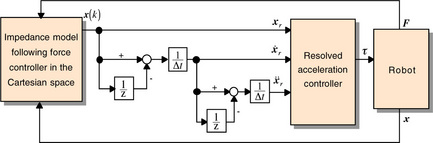
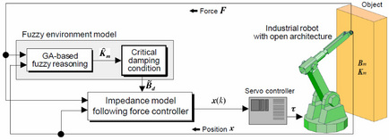
To simulate the impedance model following force control method using an industrial robot model, the manipulated variable x(k) calculated from Eq. (2.6) has to be transformed into joint driving torques. Accordingly, we propose a transformation technique where x(k) is given to the reference value of the Cartesian-based servo controller. The block diagram of this transformation is illustrated in Fig. 2.1. The joint driving torques transformed from x(k) control each joint independently.
First of all, a velocity and acceleration are generated by using a discrete time k and sampling width Δt.
For example, in the case that the resolved acceleration control law is used in the servo system of an industrial robot, x(k), ![]() (k) and
(k) and ![]() (k) generated from Eqs. (2.6), (2.7) and (2.8) are respectively given to the references xr,
(k) generated from Eqs. (2.6), (2.7) and (2.8) are respectively given to the references xr, ![]() and
and ![]() of the servo system, so that the joint torques are generated from
of the servo system, so that the joint torques are generated from
where, M(θ) ∈ ℜ6 × 6 is the inertia term in joint space; J−l(θ) is the inverse matrix of Jacobian with the relation ![]() = J(θ)
= J(θ) ![]() . Kv = diag(Kvl,…, Kv6) and Kp = diag(Kp1,…, Kp6) are the gains of velocity and position, respectively.
. Kv = diag(Kvl,…, Kv6) and Kp = diag(Kp1,…, Kp6) are the gains of velocity and position, respectively. ![]() and G(θ) are the Coriolis and centrifugal forces term and gravity term in joint space, respectively. Note that θ,
and G(θ) are the Coriolis and centrifugal forces term and gravity term in joint space, respectively. Note that θ, ![]() , x and
, x and ![]() in Eq. (2.9) are actual values, i.e., controlled variables. The non-linear compensation terms H (θ,
in Eq. (2.9) are actual values, i.e., controlled variables. The non-linear compensation terms H (θ, ![]() ) and G(θ) are effective to achieve a stable control system.
) and G(θ) are effective to achieve a stable control system.
Thus, the proposed method allows us not only to implement the impedance model following force controller in the computer simulations, but also to easily apply it to industrial robots with an open-architecture control system.
2.2.3 Design of desired damping considering the dynamics of environment
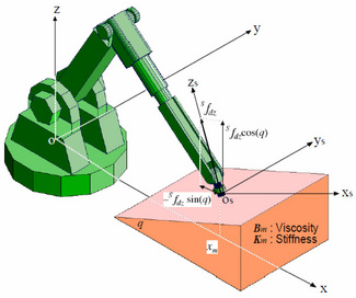
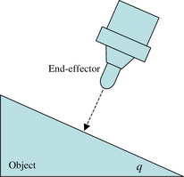
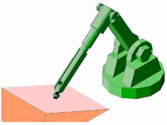
In the previous section, we have introduced the impedance model following force control for articulated industrial robots with an open-architecture controller. The problem now is how to tune the desired damping that mainly affects the force control performance. In this section we propose a tuning method of desired damping using known physical parameters. Fig. 2.2 shows an example where an industrial robot is making contact with an object inclined at q degrees from the floor. It is assumed that a stiff end-effector is fixed to the tip of the robot arm as shown in Fig. 2.3. The contact force from the normal direction of the slope is controlled to converge to a reference value Sfd. Here, the left superscript S means the value in sensor coordinate system. The end-effector is controlled to exert a small force on the object along the normal direction.
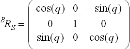
The rotation matrix in the sensor coordinate system based on the base coordinate system is described as
Therefore, the desired force vector in the base coordinate system is obtained by
For example, ![]() is transformed into
is transformed into ![]() . Here, it is assumed that the contact force f = [fx fy fz]T acting on the end-effector is represented by
. Here, it is assumed that the contact force f = [fx fy fz]T acting on the end-effector is represented by
where Bm = diag(Bm1, Bm2, Bm3) and Km = diag(Km1, Km2, Km3) are the object’s viscosity and stiffness coefficients to be positive-definite diagonal matrices. It is also assumed that the tip of the robot arm contacts the object at the position xmT = [xm ym zm]. The transition from unconstrained motion to constrained motion is simply considered by Eq. (2.12), since it has been reported that analyzing the contact force at impact with proper models is difficult and complex [17].
In force control mode, the desired damping ![]() considering the critical damping condition of Eq. (2.1) is given by
considering the critical damping condition of Eq. (2.1) is given by
Here, i(i = 1,2,3) denotes the i-th diagonal element of each matrix. When the impedance model following force controller is applied, ![]() is given as a reference of desired damping so that promising force control suppressing overshoots and oscillations can be realized. It should be noted that when this tuning method is used, physical parameters of environments, i.e. Bmi and Kmi, are indispensable to calculate
is given as a reference of desired damping so that promising force control suppressing overshoots and oscillations can be realized. It should be noted that when this tuning method is used, physical parameters of environments, i.e. Bmi and Kmi, are indispensable to calculate ![]() .
.
2.3 Influence of environmental viscosity
In this section, it is evaluated that how much influence the environmental viscosity gives to force control performance when the impedance model following force control is applied. The contact force given by Eq. (2.12) is considered under sixteen kinds of different environments where the combination of the stiffness and viscosity are shown in Tables 2.1 and 2.2, respectively. As can be seen from these tables, it is assumed that the physical characteristics in x- and z-directions are equivalent, i.e., Km1 = Km3 and Bm1 = Bm3. Force control simulations illustrated in Fig. 2.4 are conducted under above sixteen conditions. The slope angle q is set to 30°. The orientation of the end-effector is controlled to be fixed with [0 150° 0] so that the robot arm can exert the force on the surface of the slope along the normal direction. When f is obtained by Eq. (2.12), the four kinds of environmental viscosity shown in Table 2 are used. On the other hand, when the desired damping given by Eq. (2.13) is calculated, Bm is fixed to diag(15,0,15). By means of these conditions, force control schemes given by Eq. (2.6) with and without the information of environmental viscosity are compared. Simulations are carried out using the kinetic and dynamic parameters of the PUMA560 manipulator [3]. The dynamic equation is written by
Table 2.1
Stiffness of environment [N/m]
| (1) | Km1 = Km3 = 5000 |
| (2) | Km1 = Km3 = 10000 |
| (3) | Km1 = Km3 = 15000 |
| (4) | Km1 = Km3 = 20000 |
Table 2.2
Viscosity of environment [Ns/m]
| (a) | Bm1 = Bm3= 0 |
| (b) | Bm1= Bm3= 1 |
| (c) | Bm1 = Bm3 = 15 |
| (d) | Bm1 = Bm3 = 20 |
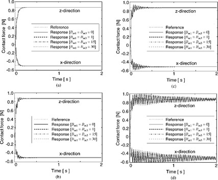
Figure 2.4 Force control results: (a)Km1 = Km3 = 5000 N/m, (b)Km1= Km3 = 10000 N/m, (c)Km1 = Km3 = 15000 N/m, (d)Km1 = Km3 = 20000 N/m
The simulation time and sampling width are set to 2 sec. and 0.01 sec., respectively. In this case, the initial contact position xm was given to the desired position xd in Eq. (2.6). The desired stiffness and force feedback gain are set to Kd1 = Kd3 = 400 N/m and Kf1 = Kf3 = 10, respectively. Fig. 2.4 show the sixteen kinds of results.
For example, Fig. 2.4(a) shows the compared results of force control responses when the combination of Bm1,Bm3 to Km1, Km3 = 5000 N/m are changed with values shown in Table 2.1. It is observed from the result that the environmental viscosity does not affect the force control performance because there is little superiority or inferiority of each response shown in Fig. 2.4(a). The similar tendency are observed also from Figs. 2.4(b)-(d). In other words, it is confirmed from these simulations that the instability of the manipulator’s force control mainly depends on the stiffness of the environment. Furthermore, it is also shown that the response becomes more unstable when the end-effector comes in contact with stiffer environments. An et al. [19] and Sasaki et al. [18] have already reported two kinds of detailed stability analysis of this behavior using a conventional force control and impedance control, respectively: the stability problem in contact with an environment is general and not limited to force control methodologies used, because the manipulated variables in most force control methods have a term consisting of the product of the environmental stiffness and force feedback gain. Therefore, the force feedback system is forced to have a high gain feedback loop, if the robot deals with a stiff environment.
When a robot comes in contact with its environment in actual tasks, there are several factors that decrease the total stiffness of the system. They are called clearance, strain and deflection, all of which exist not only in the robot itself but also in the end-effector, force sensor and so on. That is the reason why such a total stiffness should be carefully addressed in designing a robotic force control system. Hereafter, it is assumed that the environmental stiffness includes that of the robot itself. By considering these preliminary simulation results, estimating the stiffness of environment is expected to be sufficient to realize a stable force control system suppressing overshoots and oscillations. In the next section, the fuzzy environment model (FEM) that estimates the stiffness of unknown environment is proposed for the impedance model following force controller.
2.4 Fuzzy environment model
2.4.1 Design of fuzzy environment model
The fuzzy environment model (FEM), based on fuzzy reasoning theory, estimates the stiffness of environment. We design the FEM by using the simple fuzzy reasoning theory, which is regarded as a kind of model, developed by Takagi et al. [21]. In this section, we describe how to construct the FEM giving an example of force control shown in Fig. 2.2. According to the former definition, the position vector and the force vector at the tip of the robot arm are given with xT = [x(t) y(t) z(t)] and fT = [fx(t) 0 fz(t)], respectively. The motivation behind the proposed concept is to simplify the construction of the FEM, so each reasoning in the x-or z-direction is conducted independently. Fuzzy inputs for reasoning are defined by
If the information on only x-direction is used, the FEMs are described by
IF x*(t) is ![]() , THEN
, THEN ![]() + Km1 (x − xm) = − f
+ Km1 (x − xm) = − f
IF x*(t) is ![]() , THEN
, THEN ![]() + Km2 (x − xm) = − f
+ Km2 (x − xm) = − f
IF x*(t) is ![]() , THEN
, THEN ![]() + KmL (x − xm) = − f
+ KmL (x − xm) = − f
Where ![]() (i = 1,…,L) is the antecedent fuzzy set and L is the number of labels. If the x-directional element Km1 of stiffness coefficient matrix Km is estimated in parallel with above fuzzy environment models, the reasoning rules are represented by
(i = 1,…,L) is the antecedent fuzzy set and L is the number of labels. If the x-directional element Km1 of stiffness coefficient matrix Km is estimated in parallel with above fuzzy environment models, the reasoning rules are represented by
where Km1i(i = 1,…,L) denotes the consequent constant. Using these rules, the estimated stiffness ![]() in the x-direction is computed by the weighted mean method expressed as
in the x-direction is computed by the weighted mean method expressed as
where pi {x*(t)} denotes the normalized confidence given by
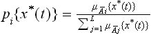
with the antecedent confidence ![]() {x∗(t)}described by the following Gaussian membership function
{x∗(t)}described by the following Gaussian membership function
where, αj is the center of membership function and βj is the reciprocal value of standard deviation, and j(j = 1,…,L) denotes the number of fuzzy rules. The Gaussian type membership function is shaped by only the center of membership function and the reciprocal value of standard deviation. In optimizing the FEM using genetic algorithms (GA), the confidence is calculated after the genotype of each FEM is decoded to the phenotype. In this case, the Gaussian type membership function allows the system to easily calculate the confidence, compared with triangular type membership functions. Because of this advantage, we use the Gaussian type membership function. The weighted mean method is generally used in the simple fuzzy reasoning method. This method requires no centroidal calculations, so that high speed operation and analysis can be realized, compared to the min-max centroidal method or the product-sum cen- troidal method. In the same manner, the estimated stiffness ![]() in the z-direction is computed by giving Eq. (2.16) to the input of fuzzy reasoning. Fig. 2.5 shows the block diagram of the impedance model following force controller with the FEM. The FEM estimates the environmental stiffness sensing the force measurements and provides the desired damping
in the z-direction is computed by giving Eq. (2.16) to the input of fuzzy reasoning. Fig. 2.5 shows the block diagram of the impedance model following force controller with the FEM. The FEM estimates the environmental stiffness sensing the force measurements and provides the desired damping ![]() based on Eq. (2.13) to maintain the system in critically damped condition. The impedance model following force controller generates the manipulated variable x(k) for the servo system with
based on Eq. (2.13) to maintain the system in critically damped condition. The impedance model following force controller generates the manipulated variable x(k) for the servo system with ![]() .
.
As can be seen from the above arguments, the key point for the design of the FEM is to appropriately adjust α, β in the antecedent part and consequent constant given by γ. However, the effective design method for such parameters has not been developed. This means that if we want to use the FEM then the complicated parameter tuning through many simulations or experiments by trial and error is unavoidable. In the remainder of this paper, we propose a systematic tuning method for the FEM using a GA approach.
2.4.2 Offline learning of FEMs using genetic algorithms
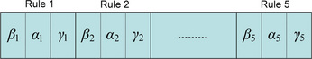
Fortunately, if the model of a manipulator used is known, then the robust FEM can be derived in advance using the GA. Before optimizing the FEM by using GA, we design the base of a FEM as follows: the type of membership functions is Gaussian; the fuzzy rule number is five; consequent parts have constant values; and so on. The GA is used to automatically adjust the parameters associated with the fuzzy rules. In other words, the GA optimizes the parameters of fuzzy rules such as the center of membership function αj, reciprocal value of standard deviation βj and constant value of consequent part γj.αj, βj and γj are the phenotypes of FEM, and each phenotype is encoded into the genotype of 16 bits binary code. An individual, i.e. a FEM, is composed of 5 fuzzy rules (L = 5) as shown in Fig. 2.6.
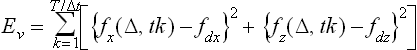
In our proposed FEM, a parameter space model deals with the viscosity and the stiffness independently. It is also assumed that the parameter space can be partitioned abstractly and formally, in which the combinations of the viscosity and the stiffness are not considered. In this case, the partition number of the parameter space is equal to the number of fuzzy rules. We empirically designed the FEM (i.e., an individual) with five fuzzy rules. For example, we can design the fuzzy labels as Further Soft, Rather Soft, Approximately Same, Rather Stiff, and Further Stiff. Of course, it is possible to use more fuzzy rules, e.g. 7 fuzzy rules for finer reasoning. Each individual is evaluated by applying the proposed method shown in Fig. 2.5 to the force control problem given in Fig. 2.2. The evaluation function Ev of each individual is the sum of squared error between the force facting on the tip of the robot arm and the reference value fd at every sampling time ∆tk, which is calculated by
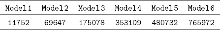
where T is the total simulation time. This is a minimization problem and therefore if the individual has the minimum Ev then it can survive as an elite. When an overshoot, oscillation or a non-contact state appears, a large dummy fitness (penalty) is given to the individual to be excluded, because such an individual is undesirable in a stable force control system. The parameters used in the GA operation are tabulated in Table 2.3. To learn the FEM, the seven kinds of environments shown in Table 2.4 are selected. Because of the aforementioned reason, the viscosity of the environments was fixed to 15 Ns/m. In addition, it was assumed that the stiffness and the viscosity of the environments have the same characteristics in x- and z-directions, respectively.
Table 2.3
| Population size | 60 |
| Number of elites | 6 |
| Selection | Tounament selection |
| Crossover | Uniform crossover |
| Mutation | Random mutation(rate=1/240) |
| Maximum generation | 100 |
Table 2.4
Stiffness of learned environments [N/m]
| (1) | Km1 = Km3 = 350 |
| (2) | Km1 = Km3 = 3500 |
| (3) | Km1 = Km3 = 7000 |
| (4) | Km1 = Km3 = 10500 |
| (5) | Km1 = Km3 = 14000 |
| (6) | Km1= Km3 = 17500 |
| (7) | Km1 = Km3 = 21000 |
Here, we examine the computational cost for learning. When a PC (CPU: Intel Celeron 1.73 GHz) is used on Windows XP Professional, it takes about 15 seconds to evaluate one individual, i.e., to integrate the dynamic model given by Eq. (2.14) for the simulation time of 2 seconds by using a Runge-Kutta algorithm. Hence, at least 15 seconds × 60 individuals × 100 generations × 7 environments = 175 hours are required to finish the whole learning.
2.4.3 Learning results
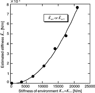
Figure 2.7 shows the relationship between the true stiffness Km1 (or Km3) of an environment and the estimated stiffness ![]() (or
(or ![]() ) in a steady state which has been obtained with best individuals. Figure 2.8 shows the relationship between the Km1 (or Km3) and the desired damping
) in a steady state which has been obtained with best individuals. Figure 2.8 shows the relationship between the Km1 (or Km3) and the desired damping ![]() (or
(or ![]() ) in the x- or z-direction given from Eq. (2.13). In Fig. 2.8, the solid lines show the desired damping (
) in the x- or z-direction given from Eq. (2.13). In Fig. 2.8, the solid lines show the desired damping (![]() :
:![]() ,
, ![]() :
:![]() ) in using
) in using ![]() and
and ![]() . On the other hand, the dotted lines represent the one (∆:
. On the other hand, the dotted lines represent the one (∆: ![]() , o:
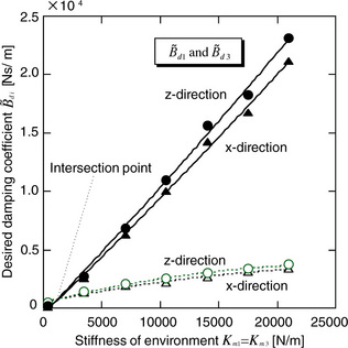
, o: ![]() ) in using Km1 and Km3 in which it is assumed that Km1 and Km3 are known. It can be observed from the result that they intersect at near the stiffness 1000 N/m. These learned results suggest that the desired damping, considering the critical damping condition with Km1 (or Km3), could achieve stable force control without overshoots and oscillations if the Km1 (or Km3) is under 1000 N/m and its neighborhood. However, if the Km1 (or Km3) is larger than the range, then a larger desired damping is needed to suppress the overshoots and oscillations. This means that if the Km1 (or Km3) becomes larger than 1000 N/m and its neighborhood, then the environmental stiffness in Eq. (2.13) must be estimated to be much larger than the true one in order to realize a desirable response. Furthermore, it can also be observed that there is a proportional relation between the real stiffness and the desired damping coefficient. It is supposed that the slope would change depending on how to evaluate and select the individuals.
) in using Km1 and Km3 in which it is assumed that Km1 and Km3 are known. It can be observed from the result that they intersect at near the stiffness 1000 N/m. These learned results suggest that the desired damping, considering the critical damping condition with Km1 (or Km3), could achieve stable force control without overshoots and oscillations if the Km1 (or Km3) is under 1000 N/m and its neighborhood. However, if the Km1 (or Km3) is larger than the range, then a larger desired damping is needed to suppress the overshoots and oscillations. This means that if the Km1 (or Km3) becomes larger than 1000 N/m and its neighborhood, then the environmental stiffness in Eq. (2.13) must be estimated to be much larger than the true one in order to realize a desirable response. Furthermore, it can also be observed that there is a proportional relation between the real stiffness and the desired damping coefficient. It is supposed that the slope would change depending on how to evaluate and select the individuals.
As an example of the learning effectiveness on seven kinds of environments, the average and minimum values of fitness are shown in Fig. 2.9, which is the evolutionary history in the case of Km1 = Km3 = 17500 N/m. It is recognized that more excellent individuals have been selected through the alternation of generations with GA operations. Figure 2.10 and Table 2.5 respectively show the antecedent membership functions and consequent constants which mean the best elite individual (a best FEM) after 100 generations. Figure 2.11 shows the simulation results using the best individual in the case of Km1 = Km3 = 17500 N/m. Figure 2.11(a) shows the force control result using the desired damping which is calculated by substituting the estimated stiffness into Eq. (2.13). Certainly, the desirable performance without overshoots and oscillations is observed. At this time, ![]() ,
,![]() and
and ![]() ,
,![]() are varied as shown in Figs. 2.11(b), (c), respectively.
are varied as shown in Figs. 2.11(b), (c), respectively.
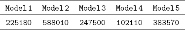
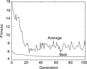
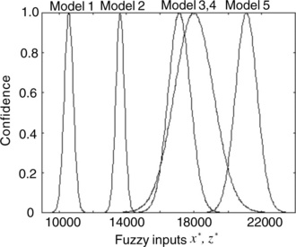
Figure 2.10 Learned antecedent membership functions (best individual) in the case of Km1 = Km3 = 17500 N/m
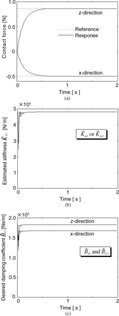
Figure 2.11 Simulation results using the best individual in the case of Km1 = Km3 = 17500 N/m: (a) force control result, (b), (c) time history of estimated stiffness ![]() ,
, ![]() and desired damping
and desired damping ![]() ,
, ![]()
It should be noted, however, that there are nonoverlapping membership functions in Fig. 2.10. In this environment, since fuzzy inputs are generated around 17500 N/m, the non-overlapping part has no impact on the response. However, the robot must deal with all supposed cases (i.e., range) in real applications, so that some flexibility (referred to as generalization) is required. At this stage, seven FEMs exist as many as the learned environments. Of course, it is not guaranteed that the desired performance can be achieved except for the learned environments. The most important function required for the FEMs is that the desired damping can be generated for all environments with any stiffness within an assumed range. In order to address this function, we consider on how to construct the learned FEMs for the generalization, where the antecedent part has no non-overlapping membership function.
2.4.4 Generalization of FEMs
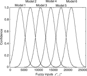
Each FEM discussed in the previous section has five fuzzy rules. If those are simply combined, then the number of fuzzy rules becomes 35 and the antecedent membership functions overlaps each other on the support set. When the combined FEMs are used, it might be that a suitable force control cannot be achieved even under a learned environment. The reason is that the fuzzy rules undesirably influence each other. Therefore, we propose a design method for the generalization which can make the FEMs work well for any environment only if the stiffness is within the range (e.g., from 3500 N/m to 21000 N/m) shown in Fig. 2.7. In order to generalize the FEMs learned under seven fixed environments, it should be considered how to interpolate the antecedent parts between two adjacent FEMs. The approach for the generalization is as follows: Although the number of learned environments is seven as shown in Table 2.4, the generalized fuzzy environment model (GFEM) is composed of six results except for Table 2.4(1) (i.e., Km1 = Km3 = 350). It is assumed that Table 2.4(1) is included in Table 2.4(2). The stiffness values of Table 2.4(2)-(7) are used for the centers of antecedent membership functions in the GFEM, and also a suitable value is given to the standard deviation of Gaussian membership functions so that there is no nonoverlapping area. On the other hand, in the design of the consequent part, the estimated stiffness coefficients shown in Fig. 2.7 are directly used for the consequent constant values.
The concrete design method is that the antecedent membership functions are placed within the range (e.g., from 3500 N/m to 21000 N/m) with the same interval as shown in Fig. 2.12, and the estimated values of environmental stiffness shown in Fig. 2.7 are set to the corresponding consequent constants. Taking account of the fact that the number of FEMs (from 3500 N/m to 21000 N/m) integrated for the generalization is six, we design the GFEM with six fuzzy rules. Km1 (or Km3) shown in Table 2.4(2)-(7) are used as the center of each membership function so that they are allocated on the support set [3500,21000] with an equal interval. Furthermore, we give 1750 to the standard deviation in order that the membership functions disposed side by side can intersect at the fitness 0.5 each other. In the design of the consequent part, the consequent models as many as the antecedent labels are prepared. The estimated stiffness coefficients, which are obtained by giving the center values of the antecedent membership functions to the horizontal values shown in Fig. 2.7, are used for the consequent constants as tabulated in Table 2.6. Fig. 2.12 and Table 2.6 show the designed antecedent membership functions and consequent constant values, respectively. The designed GFEM requires no additional acquirements and modifications of fuzzy rules during the execution of force control.
2.4.5 Results of hybrid position/force control
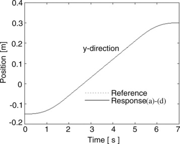
In this section, the property of robustness is proved using the impedance model following force controller with the GFEM. Here, a simple hybrid position/force control problem shown in Fig. 2.13 is conducted under the four kinds of unlearned environments shown in Table 2.7. The degree of slope is set to 30°. The contact force in the z-direction and the trajectory from point P to point Q in the y-direction in the sensor coordinate system are simultaneously controlled. To perform this task, the switch matrix S is set to diag(0, 1, 0). The desired contact force is given as
Table 2.7
Stiffness of unlearned environments [N/m]
| (a) | Kml = Km3 = 4000 |
| (b) | Km1 = Km3 = 9000 |
| (c) | Km1 = Km3 = 14000 |
| (d) | Km1 = Km3 = 19000 |
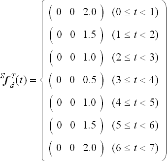
Using Eq. (2.11), SfdT(t) is transformed to fdT(t) in the base coordinate system such as
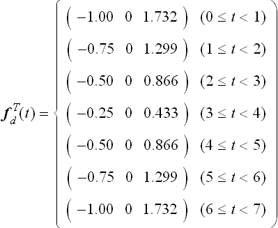
Where Z-Y-Z Euler angles, which represent the orientation of the tip of the robot arm, are fixed to [0 150° 0].
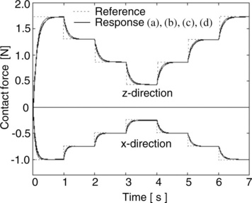
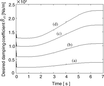
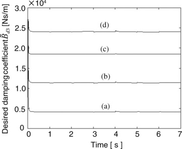
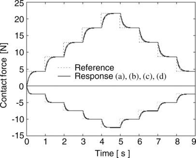
The experimental results of hybrid position/force control are shown in Figs. 2.14 and 2.15. It was confirmed that the contact forces could follow the changes of the reference without overshoots and oscillations under four environments. In this case, the desired damping coefficients in the x- and z-directions are generated from the GFEM as shown in Figs. 2.16 and 2.17, respectively. Figure 2.18 demonstrates another result, in which the desired contact force was set to larger magnitudes. From these simulation results, it was proved that the proposed GFEM could systematically generate the desired damping for stable force control even under unlearned environments.
2.5 Conclusion
In this chapter, simulations of impedance model following force control using generalized learning-based fuzzy environment model (GFEM) have been presented for articulated industrial robots with an open-architecture controller. The desired damping, which is one of the impedance parameters, has a substantial effect on force control performance, so that an important goal for successfully using the force controller is working out how to suitably tune the desired damping according to each environment and task. However, the desired damping is generally tuned by trial and error since there are no systematic tuning methods. To overcome this problem we have introduced an approach that produces the desired time-varying damping, giving the critical damping condition in contact with an object. This approach requires that the physical parameters of the object, such as viscosity and stiffness, are known beforehand.
In order to deal with unknown environments, the GFEM has been also proposed. The GFEM is designed by integrating several FEMs. Each FEM is optimized under several fixed environments in advance, using genetic algorithms. The GFEM not only estimates the stiffness of unknown environments but also systematically yields the desired time-varying damping for stable force control. The desired time-varying damping allows the impedance model following force controller to have an ability to suppress overshoots and oscillations in force control. The effectiveness and promise of the proposed method are demonstrated through hybrid position/force control simulations by using the dynamic model of a PUMA560 manipulator.
References
[1] Chen, C., Trivedi, M.M., Bidlack, C.R. Simulation and animation of sensor-driven robots. IEEE Trans. on Robotics and Automation. 1994; 10(5):684–704.
[2] Benimeli, F., Mata, V., Valero, F. A comparison between direct and indirect dynamic parameter identification methods in industrial robots. Robotica. 2006; 24(5):579–590.
[3] Corke, P. A Robotics Toolbox for MATLAB. IEEE Robotics & Automation Magazine. 1996; 3(1):24–32.
[4] Corke, P. MATLAB Toolboxes: robotics and vision for students and teachers. IEEE Robotics & Automation Magazine. 2007; 14(4):16–17.
[5] Luh, J.Y.S., Walker, M.H., Paul, R.P.C. Resolved acceleration control of mechanical manipulator. IEEE Trans. on Automatic Control. 1980; 25(3):468–474.
[6] Nagata, F., Kuribayashi, K., Kiguchi, K., Watanabe, K. Simulation of fine gain tuning using genetic algorithms for model-based robotic servo controllers. IEEE International Symposium on Computational Intelligence in Robotics and Automation. (196–201):2007.
[7] Nagata, F., Okabayashi, I., Matsuno, M., Utsumi, T., Kuribayashi, K., Watanabe, K., Fine gain tuning for model-based robotic servo controllers using genetic algorithms. 13th International Conference on Advanced Robotics. 2007:987–992.
[8] Hogan, N. Impedance control: An approach to manipulation: Part I - Part III. Transactions of the ASME, Journal of Dynamic Systems, Measurement and Control. 1985; 107:1–24.
[9] Nagata, F., Watanabe, K., Hashino, S., Tanaka, H., Matsuyama, T., Hara, K., Polishing robot using a joystick controlled teaching system. IEEE International Conference on Industrial Electronics, Control and Instrumentation. 2000:632–637.
[10] Craig, J.J. Introduction to ROBOTICS —Mechanics and Control Second Edition—. Addison Wesley Publishing Co., Reading, Mass; 1989.
[11] Nagata, F., Kusumoto, Y., Fujimoto, Y., Watanabe, K. Robotic sanding system for new designed furniture with free-formed surface. Robotics and Computer-Integrated Manufacturing. 2007; 23(4):371–379.
[12] Kawato, M. The feedback-error-learning neural network for supervised motor learning. In: Advanced Neural Computers. Elsevier Amsterdam; 1990:365–373.
[13] Nakanishi, J., Schaal, S. Feedback error learning and nonlinear adaptive control. Neural Networks. 2004; 17(10):1453–1465.
[14] Furuhashi, T., Nakaoka, K., Maeda, H., Uchikawa, Y. A proposal of genetic algorithm with a local improvement mechanism and finding of fuzzy rules. Journal of Japan Society for Fuzzy Theory and Systems. 1995; 7(5):978–987. [(in Japanese)].
[15] Linkens, D.A., Nyongesa, H.O. Genetic algorithms for fuzzy control part 1: Offline system development and application. IEE Proceedings Control Theory and Applications. 1995; 142(3):161–176.
[16] Linkens, D.A., Nyongesa, H.O. Genetic algorithms for fuzzy control part 2: Online System Development and Application. IEE Proceedings Control Theory and Applications. 1995; 142(3):177–185.
[17] Ferretti, G., Magnani, G., Zavala Rio, A. Impact modeling and control for industrial manipulators. IEEE Control Systems Magazine. 1998; 18(4):65–71.
[18] Sasaki, T., Tachi, S. Contact stability analysis on some impedance control methods. Journal of the Robotics Society of Japan. 1994; 12(3):489–496. [(in Japanese)].
[19] An, H.C., Hollerbach, J.M., Dynamic stability issues in force control of manipulators. IEEE International Conference on Robotics and Automation. 1987:890–896.
[20] An, H.C., Atkeson, C.G., Hollerbach, J.M., Model-based control of a robot manipulatorThe MIT Press classics series. Massachusetts: The MIT Press, 1988.
[21] Takagi, T., Sugeno, M. Fuzzy identification of systems and its applications to modeling and control. IEEE Transactions Systems, Man & Cybernetics. 1985; 15(1):116–132.
[22] Nagata, F., Watanabe, K., Sato, K., Izumi, K., An experiment on profiling task with impedance controlled manipulator using cutter location data. IEEE International Conference on Systems, Man, and Cybernetics. 1999:848–853.
[23] Nagata, F., Watanabe, K., Izumi, K., Furniture polishing robot using a trajectory generator based on cutter location data. IEEE International Conference on Robotics and Automation. 2001:319–324.
[24] Raibert, M.H., Craig, J.J. Hybrid position/force control of manipulators. Transactions of the ASME, Journal of Dynamic Systems, Measurement and Control. 1981; 102:126–133.
[25] Nagata, F., Hase, T., Haga, Z., Omoto, M., Watanabe, K. CAD/CAM-based position/force controller for a mold polishing robot. Mechatronics. 2007; 17(4/5):207–216.
[26] Nagata, F., Watanabe, K., Hashino, S., Tanaka, H., Matsuyama, T., Hara, K. Polishing robot using joystick controlled teaching. Journal of Robotics and Mechatronics. 2001; 13(5):517–525.
[27] Nagata, F., Watanabe, K., Kiguchi, K. Joystick teaching system for industrial robots using fuzzy compliance control. Industrial Robotics: Theory, Modelling and Control, INTECH, pages. (799–812):2006.
[28] Maeda, Y., Ishido, N., Kikuchi, H., Arai, T., Teaching of grasp/graspless manipulation for industrial robots by human demonstration. IEEE/RSJ International Conference on Intelligent Robots and Systems. 2002:1523–1528.
[29] Kushida, D., Nakamura, M., Goto, S., Kyura, N. Human direct teaching of industrial articulated robot arms based on force-free control. Artificial Life and Robotics. 2001; 5(1):26–32.
[30] Sugita, S., Itaya, T., Takeuchi, Y. Development of robot teaching support devices to automate deburring and finishing works in casting. The International Journal of Advanced Manufacturing Technology. 2003; 23(3/4):183–189.
[31] Ahn, C.K., Lee, M.C., An off-line automatic teaching by vision information for robotic assembly task. IEEE International Conference on Industrial Electronics, Control and Instrumentation. 2000:2171–2176.
[32] Neto, P., Pires, J.N., Moreira, A.P., CAD-based offline robot programming. IEEE International Conference on Robotics Automation and Mechatronics. 2010:516–521.
[33] Ge, D.F., Takeuchi, Y., Asakawa, N. Automation of polishing work by an industrial robot, – 2nd report, automatic generation of collision-free polishing path –. Transaction of the Japan Society of Mechanical Engineers. 1993; 59(561):1574–1580. [(in Japanese)].
[34] Ozaki, F., Jinno, M., Yoshimi, T., Tatsuno, K., Takahashi, M., Kanda, M., Tamada, Y., Nagataki, S. A force controlled finishing robot system with a task-directed robot language. Journal of Robotics and Mechatronics. 1995; 7(5):383–388.
[35] Pfeiffer, F., Bremer, H., Figueiredo, J. Surface polishing with flexible link manipulators. European Journal of Mechanics, A/Solids. 1996; 15(1):137–153.
[36] Takeuchi, Y., Ge, D., Asakawa, N., Automated polishing process with a human-like dexterous robot. IEEE International Conference on Robotics and Automation. 1993:950–956.
[37] Pagilla, P.R., Yu, B. Robotic surface finishing processes: modeling, control, and experiments. Transactions of the ASME, Journal of Dynamic Systems, Measurement and Control. 2001; 123:93–102.
[38] Huang, H., Zhou, L., Chen, X.Q., Gong, Z.M. SMART robotic system for 3D profile turbine vane airfoil repair. International Journal of Advanced Manufacturing Technology. 2003; 21(4):275–283.
[39] Stephien, T.M., Sweet, L.M., Good, M.C., Tomizuka, M. Control of tool/workpiece contact force with application to robotic deburring. IEEE Journal of Robotics and Automation. 1987; 3(1):7–18.
[40] Kazerooni, H. Robotic deburring of two-dimensional parts with unknown geometry. Journal of Manufacturing Systems. 1988; 7(4):329–338.
[41] Her, M.G., Kazerooni, H. Automated robotic deburring of parts using compliance control. Transactions of the ASME, Journal of Dynamic Systems, Measurement and Control. 1991; 113:60–66.
[42] Bone, G.M., Elbestawi, M.A., Lingarkar, R., Liu, L. Force control of robotic deburring. Transactions of the ASME, Journal of Dynamic Systems, Measurement and Control. 1991; 113:395–400.
[43] Gorinevsky, D.M., Formalsky, A.M., Schneider, A.Y. Force Control of Robotics Systems. New York: CRC Press; 1997.
[44] Takahashi, K., Aoyagi, S., Takano, M., Study on a fast profiling task of a robot with force control using feedforward of predicted contact position data. 4th Japan-France Congress & 2nd Asia-Europe Congress on Mechatronics. 1998:398–401.
[45] Takeuchi, Y., Watanabe, T. Study on post-processor for 5-axis control machining. Journal of the Japan Society for Precision Engineering. 1992; 58(9):1586–1592. [(in Japanese)].
[46] Takeuchi, Y., Wada, K., Hisaki, T., Yokoyama, M. Study on post-processor for 5-axis control machining centers —In case of spindle-tilting type and table/spindle-tilting type. Journal of the Japan Society for Precision Engineering. 1994; 60(1):75–79. [(in Japanese)].
[47] Xu, X.J., Bradley, C., Zhang, Y.F., Loh, H.T., Wong, Y.S. Tool-path generation for five-axis machining of free-form surfaces based on accessibility analysis. International Journal of Production Research. 2002; 40(14):3253–3274.
[48] Chen, S.L., Chang, T.H., Inasaki, I., Liu, Y.C. Postprocessor development of a hybrid TRR-XY parallel kinematic machine tool. The International Journal of Advanced Manufacturing Technology. 2002; 20(4):259–269.
[49] Lei, W.T., Hsu, Y.Y. Accuracy test of five-axis CNC machine tool with 3D probe-ball Part I: design and modeling. Machine Tool & Manufacture. 2002; 42(10):1153–1162.
[50] Lei, W.T., Sung, M.P., Liu, W.L., Chuang, Y.C. Double ballbar test for the rotary axes of five-axis CNC machine tools. Machine Tool & Manufacture. 2006; 47(2):273–285.
[51] Cao, L.X., Gong, H., Liu, J. The offset approach of machining free form surface. Part 1: Cylindrical cutter in five-axis NC machine tools. Journal of Materials Processing Technology. 2006; 174(1/3):298–304.
[52] Cao, L.X., Gong, H., Liu, J. The offset approach of machining free form surface. Part 2: Toroidal cutter in 5-axis NC machine tools. Journal of Materials Processing Technology. 2007; 184(1/3):6–11.
[53] Timar, S.D., Farouki, R.T., Smith, T.S., Boyadjieff, C.L. Algorithms for time optimal control of CNC machines along curved tool paths. Robotics and Computer-Integrated Manufacturing. 2005; 21(1):37–53.
[54] Heo, E.Y., Kim, D.W., Kim, B.H., Chen, F.F. Estimation of NC machining time using NC block distribution for sculptured surface machining. Robotics and Computer-Integrated Manufacturing. 2006; 22(5–6):437–446.
[55] Tarng, Y.S., Chuang, H.Y., Hsu, W.T. Intelligent cross-coupled fuzzy feedrate controller design for CNC machine tools based on genetic algorithms. International Journal of Machine Tools and Manufacture. 1999; 39(10):1673–1692.
[56] Zuperl, U., Cus, F., Milfelner, M. Fuzzy control strategy for an adaptive force control in end-milling. Journal of Materials Processing Technology. 2005; 164/165:1472–1478.
[57] Farouki, R.T., Manjunathaiah, J., Nicholas, D., Yuan, G.F., Jee, S. Variable-feedrate CNC interpolators for constant material removal rates along Pythagorean-hodograph curves. Computer-Aided Design. 1998; 30(8):631–640.
[58] Farouki, R.T., Manjunathaiah, J., Yuan, G.F. G codes for the specification of Pythagorean-hodograph tool paths and associated feedrate functions on open-architecture CNC machines. Machine Tools & Manufacture. 1999; 39(1):123–142.
[59] Frank, A., Schmid, A. Grinding of non-circular contours on CNC cylindrical grinding machines. Robotics and Computer-Integrated Manufacturing. 1988; 4(1/2):211–218.
[60] Couey, J.A., Marsh, E.R., Knapp, B.R., Vallance, R.R. Monitoring force in precision cylindrical grinding. Precision Engineering. 2005; 29(3):307–314.
[61] Tawakoli, T., Rasifard, A., Rabiey, M. Highefficiency internal cylindrical grinding with a new kinematic. Machine Tools & Manufacture. 2007; 47(5):729–733.
[62] Nagata, F., Kusumoto, Y., Hasebe, K., Saito, K., Fukumoto, M., Watanabe, K., Post-processor using a fuzzy feed rate generator for multi-axis NC machine tools with a rotary unit. International Conference on Control, Automation and Systems. 2005:438–443.
[63] Nagata, F., Watanabe, K. Development of a postprocessor module of 5-axis control NC machine tool with tilting-head for woody furniture. Journal of the Japan Society for Precision Engineering. 1996; 62(8):1203–1207. [(in Japanese)].
[64] Fujino, K., Sawada, Y., Fujii, Y., Okumura, S., Machining of curved surface of wood by ball end mill – Effect of rake angle and feed speed on machined surface. 16th International Wood Machining Seminar, Part 2. 2003:532–538.
[65] Nagata, F., Hase, T., Haga, Z., Omoto, M., Watanabe, K., Intelligent desktop NC machine tool with compliance control capability. 13th International Symposium on Artificial Life and Robotics. 2008:779–782.
[66] Duffy, J. The Fallacy of modern hybrid control theory that is based on orthogonal complements of twist and wrench spaces. Journal of Robotic Systems. 1990; 7(2):139–144.
[67] Lee, M.C., Go, S.J., Lee, M.H., Jun, C.S., Kim, D.S., Cha, K.D., Ahn, J.H. A robust trajectory tracking control of a polishing robot system based on CAM data. Robotics and Computer-Integrated Manufacturing. 2001; 17(1/2):177–183.
[68] Nagata, F., Mizobuchi, T., Tani, S., Hase, T., Haga, Z., Watanabe, K., Habib, M.K., Kiguchi, K., Desktop orthogonal-type robot with abilities of compliant motion and stick-slip motion for lapping of LED lens molds. IEEE International Conference on Robotics & Automation. 2010:2095–2100.
[69] Bilkay, O., Anlagan, O. Computer simulation of stick-slip motion in machine tool slideways. Tribology International. 2004; 37(4):347–351.
[70] Mei, X., Tsutsumi, M., Tao, T., Sun, N. Study on the compensation of error by stick-slip for high-precision table. International Journal of Machine tools & Manufacture. 2004; 44(5):503–510.
[71] Tsai, M.J., Chang, J.L., Haung, J.F., Development of an automatic mold polishing system. IEEE International Conference on Robotics & Automation. 2003:3517–3522.
[72] Tsai, M.J., Fang, J.J., Chang, J.L. Robotic path planning for an automatic mold polishing system. International Journal of Robotics & Automation. 2004; 19(2):81–89.
[73] Hocheng, H., Sun, Y.H., Lin, S.C., Kao, P.S. A material removal analysis of electrochemical machining using flat-end cathode. Journal of Materials Processing Technology. 2003; 140(1/3):264–268.
[74] Uehara, Y., Ohmori, H., Lin, W., Ueno, Y., Naruse, T., Mitsuishi, N., Ishikawa, S., Miura, T., Development of spherical lens ELID grinding system by desk-top 4-axes Machine Tool. International Conference on Leading Edge Manufacturing in 21st Century. 2005:247–252.
[75] Ohmori, H., Uehara, Y. Development of a desktop machine tool for mirror surface grinding. International Journal of Automation Technology. 2010; 4(2):88–96.
[76] Nagata, F., Hase, T., Haga, Z., Omoto, M., Watanabe, K. Intelligent desktop NC machine tool with compliant motion capability. Artificial Life and Robotics. 2009; 13(2):423–427.
[77] Nagata, F., Tani, S., Mizobuchi, T., Hase, T., Haga, Z., Omoto, M., Watanabe, K., Habib, M.K., Basic performance of a desktop NC machine tool with compliant motion capability. IEEE International Conference on Mechatronics and Automation, WC1-5. 2008:1–6.
[78] Nagata, F., Watanabe, K., Sato, K., Izumi, K. Impedance control using anisotropic fuzzy environment models. Journal of Robotics and Mechatronics. 1999; 11(1):60–66.
[79] Nagata, F., Otsuka, A., Yoshitake, S., Watanabe, K., Automatic control of an orthogonal-type robot with a force sensor and a small force input device. The 37th Annual Conference of the IEEE Industrial Electronics Society. 2011:3151–3156.
[80] Nagata, F., Watanabe, K. Feed rate control using a fuzzy reasoning for a mold polishing robot. Journal of Robotics and Mechatronics. 2006; 18(1):76–82.
[81] Nagata, F., Watanabe, K., Japanese Patent 4094781, Robotic force control method, 2008.
[82] Nagata, F., Tsuda, K., Watanabe, K., Japanese Patent 4447746, Robotic trajectory teaching method, 2010.
[83] Tsuda, K., Yasuda, K., Nagata, F., Kusumoto, Y., Watanabe, K., Japanese Patent 4216557, Polishing apparatus and polishing method, 2008.