
Desktop orthogonal-type robot for LED lens cavities
Abstract:
In this chapter, a desktop-size orthogonal-type robot with compliance controllability is developed to finish an axis-asymmetric workpiece with multiple small concave areas. Elemental technologies such as the transformation of manipulated values from velocity to pulse, desired damping considering the critically damped condition, weak coupling control method between force and position feedback loops, stick-slip motion control method, neural network-based stiffness estimator, automatic truing of a thin wood-stick tool for long-time lapping process, and force input device for manual operation are explained in detail. The finishing performance of the proposed orthogonal-type robot is evaluated through finishing experiments of an LED lens cavity with multiple small concave areas of 4.0 mm.
7.1 Background
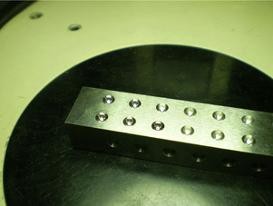
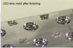
The polishing of LED lens mold after the machining process requires high accuracy, delicateness and skill, so that the process has not also been automated yet. Generally, a target mold has several concave areas precisely machined with a tolerance of ± 0.01 mm as shown in Fig. 7.1. In this case, each diameter is 4 mm. That means the target mold is not axis-symmetric, so that conventional effective polishing systems, which can deal with only axis-symmetric workpiece, cannot be applied. Accordingly, such an axis-asymmetric lens mold as shown in Fig. 7.1 is polished by skilled workers in almost all cases. Skilled workers generally polish a small lens mold using a wood-stick tool with diamond paste while checking the polished area through a microscope. However, the smaller the workpiece is, the more difficult the task. In particular, it is necessary for a pickup lens mold to handle the surface uniformly and softly, so high resolutions of position and force are indispensable. As an example of using an NC machine tool with high position resolution, Lee et al. proposed a polishing system composed of two subsystems: a three-axis machining center and a two-axis polishing robot. Although a sliding mode control algorithm with velocity compensation was implemented to reduce tracking errors, a method which could absorb undesirable positioning errors in each workpiece was not considered [67].
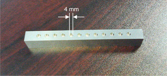
Figure 7.1 LED lens mold with several concave areas precisely machined within a tolerance, which is a typical axis-asymmetric workpiece.
In this chapter, a new desktop orthogonal-type robot with compliance controllability is presented for finishing metallic molds with small curved surfaces [65]. The orthogonal-type robot consists of three single-axis devices. A tool attached to the tip of the z-axis has a ball-end shape. Also, the control system of the orthogonal-type robot is composed of a force feedback loop, position feedback loop and position feedforward loop. The force feedback loop controls the polishing force consisting of tool contact force and kinetic friction force; the position feedback loop controls the position in the direction of spiral motion; and the position feedforward loop leads the tool tip along a spiral path. It is expected that the orthogonal-type robot delicately smooths the surface roughness with about 50 μm height on each concave area, and produces a high-quality finish for the surface.
In order to first confirm the application limit of a conventional articulated-type industrial robot to a finishing task, we evaluate the backlash that causes the position inaccuracy at the tip of the abrasive tool, through a simple position/force measurement. Through a similar position/force measurement and a surface-following control experiment along a lens mold, the basic position/force controllability of the proposed orthogonal-type robot is demonstrated.
7.2 Limitation of a polishing system based on an articulated-type industrial robot
Effective stiffness is one of the important factors to objectively evaluate the property of industrial machineries. It has already been reported that effective stiffness has a large influence on force control stability [19, 20]. Therefore, gains written in force control laws have to be tuned according to the effective stiffness so as to maintain the force control stability.
Here, as a preliminary experiment, the effective stiffness in an articulated-type industrial robot YASKAWA MOTOMAN UP6, as shown in Fig. 7.2, is examined. The arm tip has a force sensor with a stiff ball-end tool. The effective stiffness means the total stiffness including the characteristics composed of an industrial robot itself, force sensor, attachment, abrasive tool, workpiece, jig and floor. The effective stiffness, valid position resolution of Cartesian-based servo systems and resultant force resolution are evaluated simply by measuring the static position and contact force.
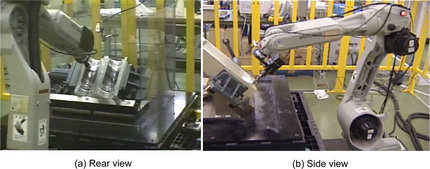
Figure 7.2 Polishing scene of a PET bottle blow mold using a conventional articulated-type industrial robot with a servo spindle.
Fig. 7.3 shows the relation between the position and contact force obtained by a simple contact experiment. The position written in the horizontal axis is the z-directional component at the tip of an abrasive tool, which is calculated by the forward kinematics using the joint angles obtained from the inner sensors. The force written in the vertical axis is yielded by contacting the tool tip with an aluminum workpiece and measured by a force sensor. When the tool tip contacts to the workpiece, small manipulated variables under 10 μm could not cause any effective force measurements,so we conducted the experiment while giving the minimum resolution − 10 μm in press motion and 10 μm in unpress motion.
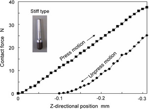
Figure 7.3 Static relation between position and contact force in case of a conventional articulated-type industrial robot.
In the experiment, the tool tip approaches an aluminum workpiece at a low speed, and after touching the workpiece, i.e., after detecting a contact force, the tool tip was pressed against the workpiece with every 0.01 mm. The graph written with ![]() in Fig. 7.3 shows the relation of the position and contact force. The force is about 36 N when the position of the tool tip is − 0.3 mm, so the effective stiffness within the range can be estimated at 120 N/mm. After the contact motion, the tool tip was away from the workpiece once, and returned to the position again where 36 N had been obtained. After that, the tool tip was unpressed every 10 im. The graph written with • in Fig. 7.3 shows the relation of the position and contact force of this case. It is observed from the result that there exists a large backlash around 0.1 mm. This value is almost the same as the general one that is guaranteed as a repetitive position accuracy of articulated-type industrial robots. That is the reason why in order to design a polishing system using an articulated-type industrial robot we must consider a force control system with the force resolution of 1.2 N under a position uncertainty of 0.1 mm. A little nonlinearity in unpress motion is also observed from the graph. The undesirable backlash and nonlinearity should be suitably eliminated or dealt with when a force control system is employed in the robot as shown in Fig. 7.2.
in Fig. 7.3 shows the relation of the position and contact force. The force is about 36 N when the position of the tool tip is − 0.3 mm, so the effective stiffness within the range can be estimated at 120 N/mm. After the contact motion, the tool tip was away from the workpiece once, and returned to the position again where 36 N had been obtained. After that, the tool tip was unpressed every 10 im. The graph written with • in Fig. 7.3 shows the relation of the position and contact force of this case. It is observed from the result that there exists a large backlash around 0.1 mm. This value is almost the same as the general one that is guaranteed as a repetitive position accuracy of articulated-type industrial robots. That is the reason why in order to design a polishing system using an articulated-type industrial robot we must consider a force control system with the force resolution of 1.2 N under a position uncertainty of 0.1 mm. A little nonlinearity in unpress motion is also observed from the graph. The undesirable backlash and nonlinearity should be suitably eliminated or dealt with when a force control system is employed in the robot as shown in Fig. 7.2.
Unfortunately, the backlash of about 0.1 mm in Cartesian space is a unpreferable property for the articulated-type industrial robot, however, it is too difficult to decrease the value. Accordingly, for example, it is almost impossible for the industrial robot to finish an LED lens mold which has the several small machined areas precisely arranged within the tolerance of 0.01 mm as shown in Fig. 7.1. The diameter of one concave area is 4.0 mm.
7.3 Desktop orthogonal-type robot with compliance controllability
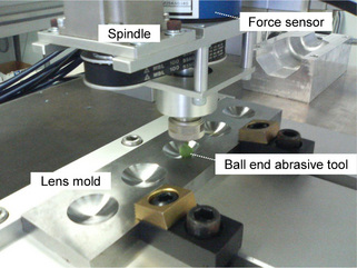
In order to polish a small concave area as shown in Fig. 7.1, a novel polishing system is proposed in this section. Fig. 7.4 shows the proposed desktop orthogonal-type robot consisting of three single-axis devices with a position resolution of 1 μm. The three single-axis devices are used for x-, y- and z-directional motions. A servo spindle motor is also used for the rotational motion of the tool axis. A compact three-DOFs force sensor is fixed between the z-axis and the attachment of the tool. The servo spindle motor with a reduction gear and the tool axis work together with a belt. The size of the robot is 850 × 645 × 700 mm. The single-axis device is a position control robot ISPA with high-precision resolution provided by IAI Corp., which is composed of a base, linear guide, ball-screw, AC servo motor and so on. The effective strokes in x-, y- and z-directions are 400, 300 and 100 mm, respectively. The hardware block diagram is shown in Fig. 7.5.
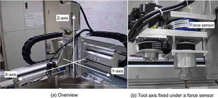
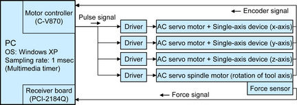
Figure 7.5 Hardware block diagram of the desktop orthogonal-type robot composed of three single-axis devices with a position resolution of 1 μm.
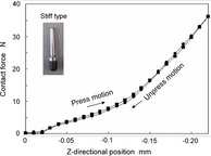
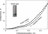
Fig. 7.6 shows the static relation between position and contact force in the case of the proposed orthogonal-type robot with a stiff ball-end abrasive tool. The experiment was conducted in the same condition as shown in Fig. 7.3. It is observed that the undesirable backlash is largely decreased and the effective stiffness is about 30/0.2 = 150 N/mm. On the other hand, Fig. 7.7 shows the relation in the case that an elastic ball-end abrasive tool is used. It is observed that the effective stiffness changes down to about 30/0.36 ≈ 83.3 N/mm according to the property of the elastic abrasive tool. As can be seen, the effective stiffness of the force control system is largely affected by the kinds of the abrasive tool used. In the case of the elastic abrasive tool called a rubber abrasive tool, it is expected that the force resolution about 0.083 N can be performed due to the position resolution of 1 μm.
7.4 Transformation technique of manipulated values from velocity to pulse
From the viewpoints of programming interface, torque command, position command and pulse command are available for the control of servo motors. Recently, a position-based servo controller in Cartesian coordinate system is provided for articulated-type industrial robots with an open-architecture, such as KAWASAKI FS20, MITSUBISHI PA10 and YASKAWA MOTOMAN UP6. The position manipulated values less than the repetitive position resolution guaranteed, e.g. 0.1 mm, are valid and can be given to the servo controller with “float” type or “double” type data in the C programming language. On the other hand, the pulse-based servo controller is widely spread to the mechatronics field because of its performance and easiness of the treatment, and is also employed in the servo motor to control each axis in the proposed NC machine tool. The pulse-based servo controller transforms the pulse command into the motor driving torque.
However, when realizing a precise position control system by using the pulse-based servo controller, a relationship between one pulse and the corresponding minimum resolution should be noted. The position control of a single axis of the robot is performed by the number of pulses, and the relative position per one sampling time can be regarded as the velocity. For example, assume that the minimum resolution in position is 1 μm for a single axis of the robot, i.e., the robot can move 1 μm by one pulse. In this case, the single-axis of the robot does not move, even if the manipulated value of 0.1 μm is continuously given to the pulse-based servo controller every sampling time period with 1 msec in order to achieve the velocity control of 100 μm/s. This is attributed to the fact that the pulse-servo controller generally ignores a fraction (i.e., values below one decimal point) less than one pulse.
Fig. 7.9 shows an example of the normal velocity vnormal(k) that was generated by the impedance model following force controller, according to the force error Ef (k) in the profiling control experiment. The values in Fig. 7.9 mean relative position commands (μm) per one sampling time with 1 msec. Observe that almost all values are plotted within the range of ± 1 μm. It should be noted, however, that the values less than 1 μm can not be treated with the pulse-based servo controller.
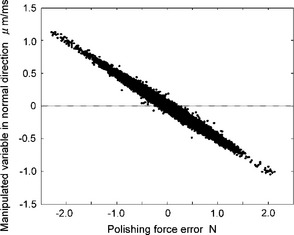
Figure 7.9 Relation between the polishing force error Ef(k) and manipulated variable vnormal(k) calculated from Eq. (4.13).
To overcome this problem, a transformation technique called the velocity-pulse conversion is proposed here. The velocity-pulse converter transforms the fine manipulated value in velocity into the pulse command given by an integer, which can be outputted to the pulse-based servo controller. The velocity-pulse converter for the pulse-based servo controller is located after the CAD/CAM-based position/force controller as shown in Fig. 7.8. Every sampling time period, to obtain the output of the velocity-pulse converter in x-direction, ![]() , calculate the summation of fractions, S(k), such as
, calculate the summation of fractions, S(k), such as
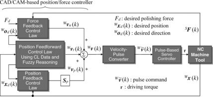
Figure 7.8 Block diagram of the CAD/CAM-based hybrid position/force controller with a velocity-pulse converter.
where Wvx(n) denotes the fraction value at time n and ki is the latest discrete time when the velocity-pulse converter generated non-zero value. If the absolute value of S(k) is greater than one, then the velocity-pulse converter generates the following pulse:
where Int(∙) is the function that extracts only the part of an integer with sign from the value of (∙). Furthermore, the fraction value should be calculated, for the next step, as
where update ki_new = k as a new nonzero output time when satisfying |S(k)| ≥ 1μm. Similarly, ![]() and
and ![]() in y- and z-directions are obtained. Thus, applying the proposed velocity-pulse converter, the velocity vector Wv(k) for Cartesian-based servo controller can be transformed into the pulse command vector
in y- and z-directions are obtained. Thus, applying the proposed velocity-pulse converter, the velocity vector Wv(k) for Cartesian-based servo controller can be transformed into the pulse command vector ![]() which can be given to the pulse-based servo controller.
which can be given to the pulse-based servo controller.
7.5 Desired damping considering the critically damped condition
The tool tip is basically controlled similar to the mold polishing robot in the previous chapter. Next, a tuning method of desired damping is proposed by using the effective stiffness of the robot. When the polishing force is controlled, the characteristics of force control system can be varied according to the combination of impedance parameters such as desired mass and desired damping. In order to increase the force control stability the desired damping, which has much influence on force control stability, should be tuned suitably. In this section, a desired damping tuning method using the effective stiffness of the robot is proposed based on the critically damped condition. When the force control mode is selected in a direction, the desired impedance model is simply written by
where ![]() ,
, ![]() and F are the acceleration, velocity and force scalars in the direction of force control, respectively.
and F are the acceleration, velocity and force scalars in the direction of force control, respectively. ![]() ,
, ![]() and Fd are the desired acceleration, velocity and force, respectively. When the force control is active,
and Fd are the desired acceleration, velocity and force, respectively. When the force control is active, ![]() ,
, ![]() and are set to zero. It is assumed that F is the external force given by the environment and is model as
and are set to zero. It is assumed that F is the external force given by the environment and is model as
where Bm and Km are the viscosity and stiffness coefficients of the environment, respectively. Eqs. (7.4) and (7.5) lead to the following second order lag system.
The characteristics equation of Eq. (7.6) is written by
In this case, the damping coefficient ζ and natural frequency ωn are given by
Further, solving Eq. (7.7) for Bd using the critical damping condition, the following condition is obtained.
Thus Hurwitz stability criterion leads to the following two relations.
Because Md, Bd and Kf are all set to positive values in advance, and Km and Bm generally have positive values. Accordingly, it is confirmed that the force control system is asymptotically stable.
In the profiling control experiment, the base value for the desired damping is calculated with Eq. (7.9). If possible, the desired damping should be fine-tuned and varied around the base value because Km has nonlinear characteristics as shown in Fig. 7.6 or 7.7.
7.6 Design of weak coupling control between force feedback loop and position feedback loop
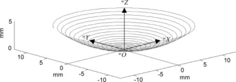
A skillful control strategy is proposed as a control strategy for LED lens molds with aspherical surfaces. An abrasive tool moves along a spiral path as shown in Fig. 7.10 while keeping the polishing force stable. The weak coupling controller has been already proposed for the PET bottle polishing robot, in which the force feedback loop and position feedback loop are coupled in a selected direction such as pick feed direction. In this case, a zigzag path is generally used for the desired trajectory, so that a position feedback control is active only in the pick feed direction, e.g., y-direction. On the contrary, in the case of the spiral path for an LED lend mold as shown in Fig. 7.10, the directions of the position feedback loops must be changed gradually all the time when the abrasive tool contacts the center of the workpiece and rises along the spiral path. Since the contact force is given to the normal direction at the contact point, the following three conditions are considered.
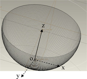
1. Around the bottom area in Fig. 7.10, the x- and y- directional components of the normal vector are almost 0. Therefore the force feedback control system should be constructed in z-direction, and the position feedback control system also should be given to the x- and y-directions.
2. Around the upper area in which the z-directional component of the normal vector is almost 0, so that the direction of the force control system should be changed x- and y-directions according to the spiral path. The position feedback control system is assigned only in the z-direction.
3. Around the middle area, the x-, y- and z-directional components of the normal vector changes every moment along the spiral path, so that the force feedback control system should be designed in x-, y- and z- directions.
The coupling control is not needed in cases 1 and 2. In case 3, however, the weak coupling control is indispensable if the the regular pick feed motion in z-direction is to be realized while performing the stable polishing force. Furthermore, it is important to independently regulate the weight of the coupling control coping with the shape of the workpiece. To deal with the problem, each component of the position feedback gain Kp = diag(Kpx, Kpy, Kpz) is varied by
where Kp is the basic gain for the weak coupling control. nz (0 < nz < 1) is the z-directional component of the normal direction vector calculated by using CL data. When the abrasive tool rises along the spiral path, nz varies from 1 to0. For example, if Kp is given the value 0.001, Kpx and Kpy varies from 0.001 to 0, and Kpz varies from 0 to 0.001.
7.7 Basic experiment
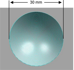
In this section, the fundamental performance of the proposed desktop orthogonal-type robot is evaluated with respect to force control and position control. A profiling control experiment is conducted by using a plastic lens mold as shown in Fig. 7.11. The target mold is precisely machined based on the forms as shown in Fig. 7.11, where the diameter and depth under the partition line are 30 mm and 5 mm, respectively. At the start of the experiment, an elastic small ball-end abrasive tool approaches to the center of machined part with 2 mm/s. After detecting 5 N, which is 1/2 of the desired polishing force 10 N, the tool tip starts to follow a spiral path. Control parameters in the profiling control are tabulated in Table 7.1. The effective stiffness Km is estimated 30/0.36 ≈ 83.3 N/mm from Fig. 7.7 in case of the elastic ball-end abrasive tool. The desired mass Md and force feedback gain Kf are set to 0.01, respectively. Also, it is assumed that Kf Bm ≈ 0 since the viscosity of the force control system is considerably small. Accordingly, Eq. (7.8) leads to Bd = 0.183 N∙s/mm.
Table 7.1
Parameters tuned for profiling control experiment.
| Conditions | Values |
| Robot | Orthogonal-type robot |
| Force sensor | NITTA IFS-67M25A |
| Desired trajectory along curved surface | Spiral path |
| Pitch in X—Y plane | 0.8 mm |
| Radius of ball-end abrasive tool R | 5 mm |
| Grain size of abrasive tool | ⋕220 |
| Desired polishing force Fd | 10 N |
| Tangent directional velocity ||vt|| | 5 mm/s |
| Desired mass coefficient Md | 0.01 N∙s2 /mm |
| Desired damping coefficient Bd | 0.183 N∙s/mm |
| Force feedback gain Kf | 0.01 |
| Diagonal elements of switch matrix Sp | 0, 0,1 |
| Position feedback gain Kpx, Kpy, Kpz | 0, 0, 0.001 |
| Integral control gain Kix, Kiy, Kiz | 0, 0, 0.00001 |
| Sampling time ∆t | 1 ms |
Next, control systems in x-,y- and z-directions are explained. The polishing force and z-directional position are regulated by feedback control laws, and also x- and y- directional positions are feedforwardly controlled based on CL data. The CL data (which are the desired trajectory) form a spiral path with a 0.8 mm pitch viewed in x-y plane. Fig. 7.12 shows the profiling control. Also, Fig. 7.13 shows the position control result, in which the pitch in x-y plane at the height 4 mm becomes about 0.7 mm. This is caused because the manipulated variable from the force feedback control law gradually yields in x- and y- directions when the tool goes up along the spiral path. In other words, the reason is that only the z-direction is designed with a position closed loop, so that the positions in x- and y-directions are corrected by the manipulated variable of the force control system, i.e., by the constraint of the force control system.
Also, the z-directional position was designed with a weak closed loop using small PI gains, so that a weak coupling was conducted against to the force feedback loop. In spite of such a situation, the mean error of z-directional position in the profiling motion was about 2.7 μm. The mean error of z-directional position was evaluated by
where N is the total step number in CL data, i.e., the number of ’GOTO’ statement. xdz(n) is the z-directional component at the n step in CL data, xz (k) is the z-directional position at the tool tip obtained from an encoder. k is the discrete time when the xdz(n) is set.
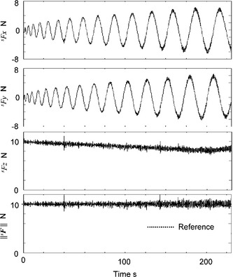
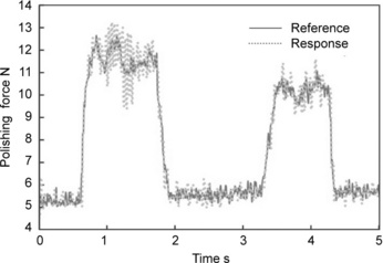
Fig. 7.14 illustrates the control result of the polishing force. The upper, second and third figures show x, y- and z-directional forces in sensor coordinate system, respectively. The lower figure shows the norm ![]() . It is observed from the SFx and SFy in Fig. 7.14 that the direction of force control periodically varies due to the position control along the spiral path. Also, although the force measurements in x- and y-directions increase with the rise of the tool and the z-directional force one decreased gradually, it can be confirmed that the polishing force ||SF|| could satisfactorily follow the reference value 10 N. The cutoff frequency of the force sensor was set to 500 Hz. Fig. 7.9 shows the normal velocity vnormal (k) which the impedance model following force controller generated according to the force error Ef(k) in the profiling control experiment. The values in Fig. 7.9 mean relative position commands μm per sampling time of 1 ms.
. It is observed from the SFx and SFy in Fig. 7.14 that the direction of force control periodically varies due to the position control along the spiral path. Also, although the force measurements in x- and y-directions increase with the rise of the tool and the z-directional force one decreased gradually, it can be confirmed that the polishing force ||SF|| could satisfactorily follow the reference value 10 N. The cutoff frequency of the force sensor was set to 500 Hz. Fig. 7.9 shows the normal velocity vnormal (k) which the impedance model following force controller generated according to the force error Ef(k) in the profiling control experiment. The values in Fig. 7.9 mean relative position commands μm per sampling time of 1 ms.
7.8 Frequency characteristics
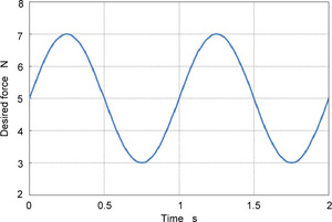
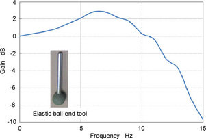
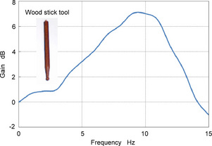
Next, the frequency characteristics of the force control system are evaluated through a simple force control experiment. Two types of tools attached to the tip of the spindle are the elastic ball-end tool (ϕ = 10 mm) and wood-stick tool (ϕ = 1 mm). Fig. 7.15 shows an example of the desired force, the frequency of which is set to 1 Hz. The peak-to-peak value of desired force is 4 N. The frequency characteristics are measured within the range from 0 Hz to 15 Hz in this order. The frequency of 0 Hz means that the desired force is set to the constant value 5 N. Figures 7.16 and 7.17 show the frequency characteristics of magnitude in the cases of the elastic ball-end abrasive tool and wood-stick tool, respectively. Although 0 dB is the ideal result in the force control system, results of more than 0 dB tend to occur with the increase of frequency. This phenomena is caused by undesirable overshots and oscillations in the stiff force control system. However, the desired polishing force in actual finishing tasks is generally set to a constant value, so that the frequency characteristics are almost no problem.
7.9 Application to finishing an LED lens mold
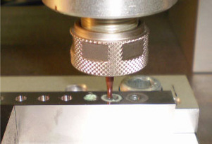
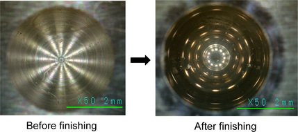
In this section, the proposed system is applied to the finishing of the LED lens mold as shown in Fig. 7.1. A small ball-end tool lathed from a wood stick is used, the tip diameter of which is 1 mm. Other parameters further tuned for the LED lens mold finishing are tabulated in Table 7.2. Fig. 7.18 shows the finishing scene of the LED lens mold, into which a special oil including the diamond lapping paste is poured. Fig. 7.19 shows the surfaces before and after the finishing process. A large-scale photo before finishing process is also shown in Fig. 7.20. It is observed that the concave surface area is of an extremely good quality like a mirror surface reflecting the room lights. Although oily spots are also observed, they can be cleaned easily.
Table 7.2
Parameters further tuned for the LED lens finishing.
| Conditions | Values |
| Desired trajectory along curved surface | Spiral path |
| Pitch of CL data viewed in X—Y plane | 0.01 mm |
| Radius of ball-end abrasive tool R | 1 mm |
| Grain size of diamond lapping paste | 4 μm |
| Desired polishing force Fd | 5 N |
| Tangent directional velocity ||vt|| | 0.1 mm/s |
| Tool revolution per minute | 400 rpm |

7.10 Stickslip motion of tool
In this section, the effectiveness of the tool’s stick-slip motion is evaluated to improve the surface quality [68]. Fig. 7.21 shows the image of the stickslip motion. Generally, the stickslip motion is an undesirable phenomenon and should be eliminated [69, 70]. However, the proposed orthogonal type robot employs a small stick-slip motion to improve the finishing quality. The stick-slip motion is given along curved surface and also to orthogonal directions of tool profiling velocity Wvt(k), i.e., tangential velocity. Here, how to generate small stick-slip motion vectors is explained in detail by using Fig. 7.22. In Fig. 7.22, point O is the origin in work coordinate system, where the tool tip initially contacts the workpiece. Point P is the current contact point. p = [px py pz]T is the position vector viewed from O; n = [nx ny nz]T is the normalized normal vector at the point P; t = [tx ty tz]T is the tangential vector at the point P; vv = [vvx vvy vvz]T is the small stickslip motion vector. In this example, the tool approaches to the workpiece with a low speed and follow the spiral path after contacting the point O. Because vv is perpendicular to n, the following relation is obtained.
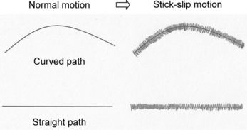
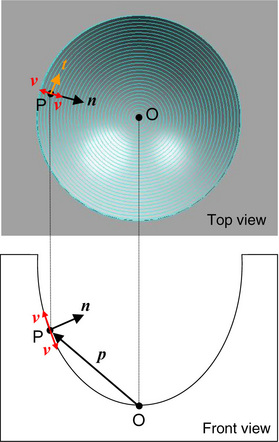
Figure 7.22 Surface of the LED lens mold before and after the finishing process. The diameter is 4 mm.
Also, vv and t are orthogonal each other, so that
Further, vv is located in a plane which includes both n and p, so that the components of vv are represented by
where i and j are the real numbers. Substituting Eqs. (7.19), (7.20) and (7.20) into Eq.(7.16) leads to
Accordingly, by giving Eq. (7.21) to Eqs. (7.17), (7.19) and (7.20), the following equations are obtained.
Because both n and p are known, vv is normalized as vv/||vv||. By using a gain kv, the stick-slip motion vector is finally obtained as kvvv/||vv||. kvvv/||vv|| is a velocity vector to yield a novel polishing energy, and which is given to the tool alternatively changing the sign every sampling period.
Next, the effectiveness of the stickslip motion control is examined through an actual finishing test. Fig. 7.23 shows a workpiece of an LED lens mold after the conventional finishing process. Although the workpiece may seem to be a high-quality surface, spotted areas are observed as shown in Fig. 7.24 in which cusps still remain. Fig. 7.25 shows a large-scale photo of the LED lens mold after the finishing process using the proposed stickslip motion control. It is observed that the undesirable cusp marks can be removed uniformly. It has been confirmed from the results that the proposed finishing strategy using the stick-slip motion control has significant effectiveness to achieve a higher-quality surface.


7.11 Neural Network-Based Stiffness Estimator
7.11.1 Nonlinear effective stiffness
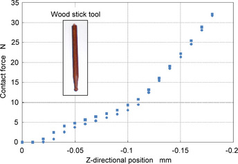
In this section, an impedance model following force control (IMFFC) using neural networks is proposed to deal with the nonlinear effective stiffness. In advance, the nonlinearity is examined by a simple static position and force measurement. The effectiveness stiffness is easily obtained by the measurement. The desired damping in IMFFC is statically calculated from the critically damped condition of the force control system. The neural networks learn the relation between the contact force and effective stiffness, so that the desired damping can be dynamically generated according to the contact force. The effectiveness is demonstrated by experiments using the orthogonal-type robot. Fig. 7.26 shows the static relation between the position and contact force obtained by a simple contact experiment. The quantity of the position is the z-directional component at the tip of a wood-stick tool. The quantity of force is yielded by contacting the tool tip with a workpiece and measured by the force sensor. The experiment was conducted while giving the relative position − 0.01 mm in press motion and 0.01 mm in unpress motion. In the experiment, the tool tip approaches an aluminum workpiece with a low speed, and after touching the workpiece, i.e., after detecting a small contact force, the tool tip was pressed to the workpiece with every 0.01 mm. The graph drawn as ![]() in Fig. 7.26 shows the relation the position and contact force. After the press motion, the tool tip was away from the workpiece once, and returned to the position again where 32 N had been obtained. After that, the tool tip was unpressed every 0.01 mm. The graph drawn as • in Fig. 7.26 shows the relation of the position and contact force of this case. It is observed that a small backlash exists. Also, the force is about 32 N when the position of the tool tip is − 0.18 mm, so that the effective stiffness within the range can be estimated as 177.7 N/mm. It is expected that a force resolution of about 0.178 N can be performed due to a position resolution of 1 μm. It has been confirmed from the experimental results that orthogonal-type robot has un- preferable nonlinearity and hysteresis. The effective stiffness is largely affected by the kinds of abrasive tools used.
in Fig. 7.26 shows the relation the position and contact force. After the press motion, the tool tip was away from the workpiece once, and returned to the position again where 32 N had been obtained. After that, the tool tip was unpressed every 0.01 mm. The graph drawn as • in Fig. 7.26 shows the relation of the position and contact force of this case. It is observed that a small backlash exists. Also, the force is about 32 N when the position of the tool tip is − 0.18 mm, so that the effective stiffness within the range can be estimated as 177.7 N/mm. It is expected that a force resolution of about 0.178 N can be performed due to a position resolution of 1 μm. It has been confirmed from the experimental results that orthogonal-type robot has un- preferable nonlinearity and hysteresis. The effective stiffness is largely affected by the kinds of abrasive tools used.
7.11.2 Learning of nonlinearity of effective stiffness
The orthogonal-type robot has a CAD/CAM-based position/force controller. The force control method used is called the impedance model following force control (IMFFC). When the force controller is applied, the desired damping should be suitably tuned according to the effective stiffness. Since unstable phenomena such as overshoot and oscillation tend to appear in the force control system with the increase of the effective stiffness, the desired damping has to use larger values. A systematic tuning method for the desired damping was already proposed in consideration of the critically damped condition in the force control system [77]. The calculation of the critically damped condition requires the effective stiffness of the force control system with nonlinearity [78]. Fig. 7.27 shows the nonlinear variation of effective stiffness in press and unpress motions obtained from Fig. 7.26. The number of measured points is 19, respectively.
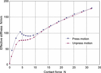
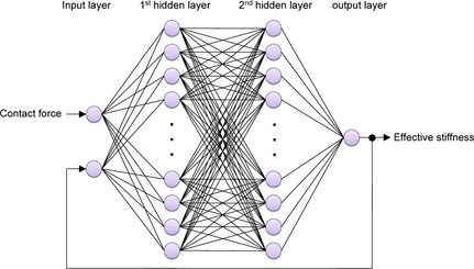
In this subsection, three examples of nonlinearity have been introduced, in which a stiff abrasive tool, an elastic abrasive tool and a thin wood-stick tool are used. As can be seen, the orthogonal-type robot has to deal with many kinds of abrasive tools with both different nonlinearity and hysteresis. In order to deal with the nonlinearity as shown in Fig. 7.27, a recurrent neural network (RNN) is employed as shown in Fig. 7.28. The RNN is chosen for the proposed robot in consideration of the following generally-known four reasons.
1. A multi-layered neural network works as an effective nonlinear regression model.
2. The learning method known as the back propagation algorithm is simple to implement in software. The learning result obtained as an input/output model can also easily be applied to the control system.
3. The learned RNN has a promising generalization ability for unlearned input data.
4. It has a superior extensibility to a multi-input and multi-output system.
In order to make a map of a single-input and single-output system, a straightforward method based on the sampling points shown in Fig. 7.27 is to use linear functions to interpolate them. However, when the system is extended to a multi-input and single-output system, the NN-based design will perform more suitable role. In the first subsection, in order to compare with the property of a conventional industrial robot that had already been tested in section 8.2, a simple static effective stiffness of the orthogonal-type robot was similarly measured. As a next step, it is planned to measure a dynamic effective stiffness and to utilize the model in the controller. When the dynamic effective stiffness is modeled, the corresponding NN is designed as a three-input and single-output system. The inputs are contact force, its rate and velocity in force control, and the output is the dynamic effective stiffness. That is the reason why the NN-based design has been selected from the initial stage of the development. In the proposed orthogonal-type robot, two RNNs are used for press motion and unpress motion. Each RNN consists of an input layer, two hidden layers and an output layer. Each layer has 2, 30 and 1 unit(s), respectively. Each unit is activated by a sigmoid function. Note that the output layer does not have an activate function, i.e., sigmoid function. Therefore, the RNN yields an estimated effective stiffness from the calculation of weighted sum. The RNN acquires the relation between the contact force and the effective stiffness shown in Fig. 7.27 by back propagation algorithm. Teaching patterns are given in the order left to right on the horizontal axis in Fig. 7.27.
7.11.3 NN-based effective stiffness estimator
Fig. 7.31 shows a detailed block diagram of the force feedback control law illustrated in Fig. 7.8. Fig. 7.32 also shows the detailed block diagram of the NN-based effective stiffness estimator illustrated in Fig. 7.31. The two NNs in Fig. 7.32 are switched by the sign of
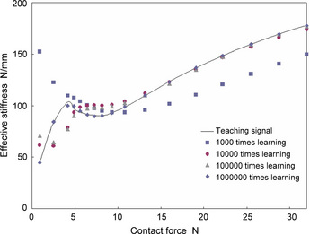
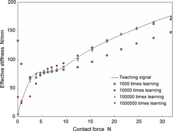
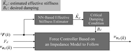
Figure 7.31 Block diagram of the force feedback control law shown in Fig. 3.4.
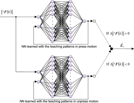
Figure 7.32 Detailed block diagram of the NN-based effective stiffness estimator shown in Fig. 7.31.
If Δ||SF(k)|| > 0, then a NN learned with the teaching patterns in press motion is selected, whereas, if Δ||SF(k)|| < 0, then NN learned with the teaching patterns in unpress motion is used. For example, when the desired polishing force Fd is set to 10 N, the points of 10 N in Figs. 7.29 and 7.30 become the operating points. The NN-based effective stiffness estimator generates time-varying effective stiffness ![]() around the operating points. In the next example, a critically damped condition in the force control system generates the desired damping for stable force control.
around the operating points. In the next example, a critically damped condition in the force control system generates the desired damping for stable force control.
Fig. 7.33 shows the example, in which the polishing force is successfully controlled around 20 N in spite of oscillations caused by a tool rotation of 400 rpm. In this case, it is observed that the NN-based effective stiffness estimator yielded the effective stiffness ![]() as shown in Fig. 7.34. Since the viscosity Bm in Eq. (7.9) could be regarded as zero, the desired damping was calculated with
as shown in Fig. 7.34. Since the viscosity Bm in Eq. (7.9) could be regarded as zero, the desired damping was calculated with ![]() as given by
as given by
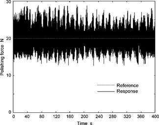
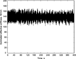
Figure 7.34 Effective stiffness ![]() estimated by the neural networks illustrated in Fig. 7.32
estimated by the neural networks illustrated in Fig. 7.32
7.12 Automatic Tool Truing for Long-Time Lapping Process
When a polishing compound such as a diamond paste is used, the finishing or polishing process is called the lapping process. It is not easy to automate the lapping process of a metallic LED lens cavity because the cavity itself is not axis-symmetric and a lot of concave areas on the cavity to be finished are very small, e.g., each diameter is 4 mm. Tsai et al. developed a novel mold-polishing robot [71] and its path-planning technique [72], however, the applicability to the lapping process of an axis-asymmetric LED lens cavity was not described. We could not find previous literature concerning the finishing of an axis-asymmetric LED lens cavity. That is the reason why such an LED cavity is being dexterously finished by the hand lapping of a skilled worker in the related industrial field. However, hand lapping over a long period of time cannot be successfully carried out even by a skilled worker, consequently, defective products caused by the dispersion of quality tend to occur.
Recently, desktop-type machine tools have been developed for various industrial machining fields [73-75]. In the previous section, a computer-controlled orthogonal-type robot has been proposed to finish a concave area on an LED cavity [76]. The orthogonal-type robot is comprised of three single-axis devices with a high position resolution of 1 μm. A thin wood-stick tool is attached to the tip of the z-axis. A compact force sensor with three-DOFs is built in the z-axis. The robot has two functional applications. One is the 3D machining function, which is easily realized by using the position control mode. It is expected that the 3D machining function can be applied to the truing of a wood-stick tool. The other is the profiling function, which is performed using the hybrid position/force control mode along a spiral path. It is also expected that the profiling function can be applied to the lapping of concave areas on a metallic LED lens cavity.
We have experimentally found that a thin wood stick with a ball-end tip is very suitable for the lapping tool of an LED lens cavity. When the lapping is conducted, a special oil including diamond lapping paste, the grain size of which is about 3 μm, is poured into each concave area on the cavity. The wooden material tends to fit both the metallic material of the LED lens cavity and the diamond lapping paste due to the soft characteristics of wood compared with other conventional metallic abrasive tools. The serious problem in using a wood-stick tool is the abrasion of the tool tip. For example, an actual LED lens cavity has 180 concave areas so that the cavity can form small plastic LED lenses using mass production. However, after about five concave areas are finished, the tool tip of the wood stick is deformed from the initial ball shape as a result of the abrasion. Therefore, in order to realize a complete automatic finishing system, some truing function must be developed to systematically cope with the undesirable tool abrasion. The truing of a wood-stick tool means the reshaping to the original shape, i.e., ball-end tip.
In this section, a novel and simple automatic truing method using CL data is proposed for the long-time lapping process of an LED lens cavity and its effectiveness and validity are evaluated through an experiment. The CL data can be produced from the main-processor of 3D CAD/CAM widely used in industrial fields. The proposed orthogonaltype robot can easily carry out the truing of a wood-stick tool based on the generally-known CL data, which is another important feature of our proposed robot. The structure is very simple for the provided functions. For example, the 3D machining function is easily realized using the position control mode. Also, compliant motion to a workpiece is performed due to the profiling control mode along a desired trajectory, which will be able to be applied to the lapping process of a metallic LED lens cavity. Here, a lapping experiment is conducted to show the effectiveness of the orthogonal-type robot. And, an automatic truing function for a thin wood-stick tool is further proposed to achieve the long-time finishing process. The idea and the detailed software flowchart are described in detail.
7.12.1 Lapping experiment
The effectiveness of the orthogonal-type robot is examined through an actual lapping test of an LED lens cavity. Fig. 7.35 shows an example of a skilled worker’s hand lapping, where an LED lens cavity with multiple concave areas is being finished. The lapping process has been being required to be automated; however, its complete achievement is not easy even at the present stage.
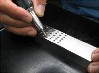
Figure 7.35 Skilled worker’s hand lapping of an LED lens cavity with multiple concave areas to be finished.
Fig. 7.36 shows the lapping scene by using the orthogonal-type robot. In this case, the polishing force acting between the tool and the LED lens cavity was successfully controlled, in which the desired value was set to 20 N. The high frequency vibrations are caused by the tool rotation of 400 rpm. Fig. 7.38 shows the surfaces before and after the lapping process. It can be observed that the undesirable cusp marks can be almost removed uniformly. It has been confirmed from the result that the proposed orthogonal-type robot has the ability to achieve a higher-quality surface.
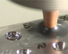
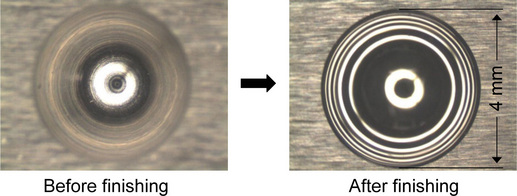
Figure 7.38 Finished surface of a concave area on an LED lens cavity, in which the controller shown in Fig. 7.32 is used.
7.12.2 Automatic on-line truing function for a thin wood-stick tool
In the previous subsection, a lapping process of an LED lens cavity is introduced as one of the applications of the proposed robot. In order to apply the robot to an actual industrial manufacturing line, the problem of the abrasion of a wood-stick tool should be overcome. Finally, an interesting and important peripheral technique is described briefly. Here, an automatic on-line truing function is proposed for the orthogonal-type robot to be able to continuously finish multiple concave areas machined on an LED lens cavity. Although the tool tip has a ball-end shape with a radius of R [mm] at the start time of the finishing, its ball shape is gradually deformed by the contour abrasion with the passage of the finishing time. Therefore, to maintain the initial performance of the tool, the truing of the tool tip plays a vital role. Fig. 7.39 shows the proposed simple scheme for an automatic wood-stick tool truing. A tool bit for automatic truing is fixed precisely on the table of the robot, so that the contour of the wood-stick tool can be easily reformed to the initial shape, i.e., the radius of R, by moving the rotating abraded tool along the trajectory from point (A) to point (B). Note that the desired trajectory written with a dotted line, where the tool with a radius of R is reversed in top and bottom, can be easily drawn by using 3D CAD, and the CL data are generated using the main-processor of the CAM.
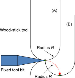
Fig. 7.40 shows the truing of a wood-stick tool, in which its desired contour shape is illustrated. The CL data used is generated within the area from point O to point P. As can be seen, the tool is being reshaped like the CAD model. The diameter of the wood-stick tool is 3 mm, so that the stiffness in the side directions is lower than the one in the vertical direction. Hence, if the truing is not conducted with a small machining force, then undesirable tool flexure will appear. The machining method used is the position feedforward control law given by Wvt(k) in the block diagram shown Fig. 7.8. It has been confirmed from the experiment that the automatic on-line truing function is successfully realized by using the proposed method.
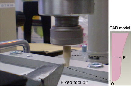
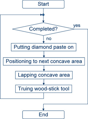
Fig. 7.41 shows the software flowchart of the orthogonaltype robot in running. First of all, if all concave areas, e.g. 180, are all finished, then the task is completed. Otherwise, the ball-end tip of the wood-stick tool puts the diamond paste on, and goes to the slightly above position of the next concave area. Then, the tool tip approaches to the concave area with a low speed of 1 mm/s. After detecting a contact with the center of the concave area, a lapping action based on the proposed control scheme starts immediately. Next, the truing of the wood-stick tool is conducted by using the method as introduced in this section, and the completion of the task is checked at the top of the flowchart. Due to the automatic truing method, the orthogonal-type robot will be able to be applied to the long-time lapping process.
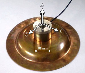
7.13 Force Input Device
Generally, when an industrial robot is used for machining, operators cannot intervene in the motion, because the motion is programmed in advance with a teaching pendant. Finally, a promising force input device is introduced for an operator to manually regulate the desired feed rate vtangent(k) as written in Eq. (6.7) or the desired polishing force Fd(k) as written in Eq. (1.17) [79]. The device is designed based on a small capacitive force sensor with three-DOFs. The force sensor is the model PD3-32-05-080 provided by Nitta Corporation. The operator’s skill can be reflected in the robotic behavior using the force input device.
The desired polishing force is varied by
where f (k) = [fx(k) fy(k) fz(k)]T is the force vector given by an operator’s finger. is the gain for decay or amplification, and Fd_base is the base value of the desired polishing force. Also, the desired feed rate, i.e, tangent velocity, is regulated by
where β is the gain for decay or amplification, and vvangent_base(k) is the output of the fuzzy feed rate generator [80]. The force sensor has three-DOFs, so that it is effective to deal with the resultant force in order to give suitable force easily and steadily by operator’s finger.
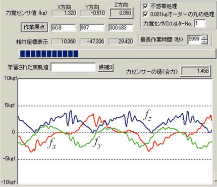
Fig. 7.43 shows the CAD/CAM-based position/force controller with the force input device to manually regulate the desired polishing force Fd(k). As an example, Fig. 7.44 shows the control result of the polishing force, in which Fd_base is set to 5 N and the desired polishing force is regulated with the force input device by an operator. As can be seen, the polishing force ||F(k)|| can follow the desired one Fd(k). Although the force input device is not equipped with any feedback factors, it is suitable for a finger tip to give small manipulated values. The operator can use the force input device while viewing the variation of the response F(k) or the force input f(k) through the dialog window as shown in Fig. 7.45.
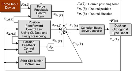
Figure 7.43 CAD/CAM-based position/force controller with the force input device to manually regulate the desired polishing force Fd(k).
7.14 Conclusion
In this chapter, we have first examined the resolution of position and force, and effective stiffness through an experiment using an automatic polishing system based on an articulated-type industrial robot with six-DOFs. Also, technical points to be improved have been considered to develop a new finishing system which can be applied to small workpieces such as an LED lens mold. Next, an orthogonal-type robot with a static position resolution of 1 μm and force resolution of 0.083 N has been designed by combining single-axis robots.
A CAD/CAM-based position/force controller with a velocity-pulse converter has been also proposed for a desktop-size orthogonal-type robot with a pulse-based servo controller, in which position control, force control or their weak coupling control can coexist together according to each finishing strategy. The velocity-pulse converter can transform minute manipulated values of velocity into a pulse command which is directly given to the pulse-based servo controller employed in various mechatronics systems.
Further, we have introduced a systematic tuning method of the desired damping. The desired damping is calculated from the critically damped condition using the static relation between the position and force. Then, a profiling control experiment using a plastic lens mold with axis symmetric surface has been conducted along a spiral path to evaluate the characteristics of position and force control. Consequently, it has been confirmed that the proposed orthogonal-type robot has a desirable control performance of position and force which would be applied to the finishing task of plastic lens molds.
Furthermore, a force input device has been introduced for an operator to manually regulate the desired feed rate or the desired polishing force. It is expected that the force input device will allow industrial machineries to realize cooperative motion between an automatic control and a manual control based on the operator’s skill, which is another important advantage of the proposed orthogonal-type robot.
In future work, we plan to develop a much smaller ballend abrasive tool for finishing a workpiece with smaller concave areas of 3.6 mm and to conduct a finishing experiment by using the proposed orthogonal-type robot with compliance controllability.
References
[1] Chen, C., Trivedi, M.M., Bidlack, C.R. Simulation and animation of sensor-driven robots. IEEE Trans. on Robotics and Automation. 1994; 10(5):684–704.
[2] Benimeli, F., Mata, V., Valero, F. A comparison between direct and indirect dynamic parameter identification methods in industrial robots. Robotica. 2006; 24(5):579–590.
[3] Corke, P. A Robotics Toolbox for MATLAB. IEEE Robotics & Automation Magazine. 1996; 3(1):24–32.
[4] Corke, P. MATLAB Toolboxes: robotics and vision for students and teachers. IEEE Robotics & Automation Magazine. 2007; 14(4):16–17.
[5] Luh, J.Y.S., Walker, M.H., Paul, R.P.C. Resolved acceleration control of mechanical manipulator. IEEE Trans. on Automatic Control. 1980; 25(3):468–474.
[6] Nagata, F., Kuribayashi, K., Kiguchi, K., Watanabe, K. Simulation of fine gain tuning using genetic algorithms for model-based robotic servo controllers. IEEE International Symposium on Computational Intelligence in Robotics and Automation. (196–201):2007.
[7] Nagata, F., Okabayashi, I., Matsuno, M., Utsumi, T., Kuribayashi, K., Watanabe, K., Fine gain tuning for model-based robotic servo controllers using genetic algorithms. 13th International Conference on Advanced Robotics. 2007:987–992.
[8] Hogan, N. Impedance control: An approach to manipulation: Part I - Part III. Transactions of the ASME, Journal of Dynamic Systems, Measurement and Control. 1985; 107:1–24.
[9] Nagata, F., Watanabe, K., Hashino, S., Tanaka, H., Matsuyama, T., Hara, K., Polishing robot using a joystick controlled teaching system. IEEE International Conference on Industrial Electronics, Control and Instrumentation. 2000:632–637.
[10] Craig, J.J. Introduction to ROBOTICS —Mechanics and Control Second Edition—. Addison Wesley Publishing Co., Reading, Mass; 1989.
[11] Nagata, F., Kusumoto, Y., Fujimoto, Y., Watanabe, K. Robotic sanding system for new designed furniture with free-formed surface. Robotics and Computer-Integrated Manufacturing. 2007; 23(4):371–379.
[12] Kawato, M. The feedback-error-learning neural network for supervised motor learning. In: Advanced Neural Computers. Elsevier Amsterdam; 1990:365–373.
[13] Nakanishi, J., Schaal, S. Feedback error learning and nonlinear adaptive control. Neural Networks. 2004; 17(10):1453–1465.
[14] Furuhashi, T., Nakaoka, K., Maeda, H., Uchikawa, Y. A proposal of genetic algorithm with a local improvement mechanism and finding of fuzzy rules. Journal of Japan Society for Fuzzy Theory and Systems. 1995; 7(5):978–987. [(in Japanese)].
[15] Linkens, D.A., Nyongesa, H.O. Genetic algorithms for fuzzy control part 1: Offline system development and application. IEE Proceedings Control Theory and Applications. 1995; 142(3):161–176.
[16] Linkens, D.A., Nyongesa, H.O. Genetic algorithms for fuzzy control part 2: Online System Development and Application. IEE Proceedings Control Theory and Applications. 1995; 142(3):177–185.
[17] Ferretti, G., Magnani, G., Zavala Rio, A. Impact modeling and control for industrial manipulators. IEEE Control Systems Magazine. 1998; 18(4):65–71.
[18] Sasaki, T., Tachi, S. Contact stability analysis on some impedance control methods. Journal of the Robotics Society of Japan. 1994; 12(3):489–496. [(in Japanese)].
[19] An, H.C., Hollerbach, J.M., Dynamic stability issues in force control of manipulators. IEEE International Conference on Robotics and Automation. 1987:890–896.
[20] An, H.C., Atkeson, C.G., Hollerbach, J.M., Model-based control of a robot manipulatorThe MIT Press classics series. Massachusetts: The MIT Press, 1988.
[21] Takagi, T., Sugeno, M. Fuzzy identification of systems and its applications to modeling and control. IEEE Transactions Systems, Man & Cybernetics. 1985; 15(1):116–132.
[22] Nagata, F., Watanabe, K., Sato, K., Izumi, K., An experiment on profiling task with impedance controlled manipulator using cutter location data. IEEE International Conference on Systems, Man, and Cybernetics. 1999:848–853.
[23] Nagata, F., Watanabe, K., Izumi, K., Furniture polishing robot using a trajectory generator based on cutter location data. IEEE International Conference on Robotics and Automation. 2001:319–324.
[24] Raibert, M.H., Craig, J.J. Hybrid position/force control of manipulators. Transactions of the ASME, Journal of Dynamic Systems, Measurement and Control. 1981; 102:126–133.
[25] Nagata, F., Hase, T., Haga, Z., Omoto, M., Watanabe, K. CAD/CAM-based position/force controller for a mold polishing robot. Mechatronics. 2007; 17(4/5):207–216.
[26] Nagata, F., Watanabe, K., Hashino, S., Tanaka, H., Matsuyama, T., Hara, K. Polishing robot using joystick controlled teaching. Journal of Robotics and Mechatronics. 2001; 13(5):517–525.
[27] Nagata, F., Watanabe, K., Kiguchi, K. Joystick teaching system for industrial robots using fuzzy compliance control. Industrial Robotics: Theory, Modelling and Control, INTECH, pages. (799–812):2006.
[28] Maeda, Y., Ishido, N., Kikuchi, H., Arai, T., Teaching of grasp/graspless manipulation for industrial robots by human demonstration. IEEE/RSJ International Conference on Intelligent Robots and Systems. 2002:1523–1528.
[29] Kushida, D., Nakamura, M., Goto, S., Kyura, N. Human direct teaching of industrial articulated robot arms based on force-free control. Artificial Life and Robotics. 2001; 5(1):26–32.
[30] Sugita, S., Itaya, T., Takeuchi, Y. Development of robot teaching support devices to automate deburring and finishing works in casting. The International Journal of Advanced Manufacturing Technology. 2003; 23(3/4):183–189.
[31] Ahn, C.K., Lee, M.C., An off-line automatic teaching by vision information for robotic assembly task. IEEE International Conference on Industrial Electronics, Control and Instrumentation. 2000:2171–2176.
[32] Neto, P., Pires, J.N., Moreira, A.P., CAD-based offline robot programming. IEEE International Conference on Robotics Automation and Mechatronics. 2010:516–521.
[33] Ge, D.F., Takeuchi, Y., Asakawa, N. Automation of polishing work by an industrial robot, – 2nd report, automatic generation of collision-free polishing path –. Transaction of the Japan Society of Mechanical Engineers. 1993; 59(561):1574–1580. [(in Japanese)].
[34] Ozaki, F., Jinno, M., Yoshimi, T., Tatsuno, K., Takahashi, M., Kanda, M., Tamada, Y., Nagataki, S. A force controlled finishing robot system with a task-directed robot language. Journal of Robotics and Mechatronics. 1995; 7(5):383–388.
[35] Pfeiffer, F., Bremer, H., Figueiredo, J. Surface polishing with flexible link manipulators. European Journal of Mechanics, A/Solids. 1996; 15(1):137–153.
[36] Takeuchi, Y., Ge, D., Asakawa, N., Automated polishing process with a human-like dexterous robot. IEEE International Conference on Robotics and Automation. 1993:950–956.
[37] Pagilla, P.R., Yu, B. Robotic surface finishing processes: modeling, control, and experiments. Transactions of the ASME, Journal of Dynamic Systems, Measurement and Control. 2001; 123:93–102.
[38] Huang, H., Zhou, L., Chen, X.Q., Gong, Z.M. SMART robotic system for 3D profile turbine vane airfoil repair. International Journal of Advanced Manufacturing Technology. 2003; 21(4):275–283.
[39] Stephien, T.M., Sweet, L.M., Good, M.C., Tomizuka, M. Control of tool/workpiece contact force with application to robotic deburring. IEEE Journal of Robotics and Automation. 1987; 3(1):7–18.
[40] Kazerooni, H. Robotic deburring of two-dimensional parts with unknown geometry. Journal of Manufacturing Systems. 1988; 7(4):329–338.
[41] Her, M.G., Kazerooni, H. Automated robotic deburring of parts using compliance control. Transactions of the ASME, Journal of Dynamic Systems, Measurement and Control. 1991; 113:60–66.
[42] Bone, G.M., Elbestawi, M.A., Lingarkar, R., Liu, L. Force control of robotic deburring. Transactions of the ASME, Journal of Dynamic Systems, Measurement and Control. 1991; 113:395–400.
[43] Gorinevsky, D.M., Formalsky, A.M., Schneider, A.Y. Force Control of Robotics Systems. New York: CRC Press; 1997.
[44] Takahashi, K., Aoyagi, S., Takano, M., Study on a fast profiling task of a robot with force control using feedforward of predicted contact position data. 4th Japan-France Congress & 2nd Asia-Europe Congress on Mechatronics. 1998:398–401.
[45] Takeuchi, Y., Watanabe, T. Study on post-processor for 5-axis control machining. Journal of the Japan Society for Precision Engineering. 1992; 58(9):1586–1592. [(in Japanese)].
[46] Takeuchi, Y., Wada, K., Hisaki, T., Yokoyama, M. Study on post-processor for 5-axis control machining centers —In case of spindle-tilting type and table/spindle-tilting type. Journal of the Japan Society for Precision Engineering. 1994; 60(1):75–79. [(in Japanese)].
[47] Xu, X.J., Bradley, C., Zhang, Y.F., Loh, H.T., Wong, Y.S. Tool-path generation for five-axis machining of free-form surfaces based on accessibility analysis. International Journal of Production Research. 2002; 40(14):3253–3274.
[48] Chen, S.L., Chang, T.H., Inasaki, I., Liu, Y.C. Postprocessor development of a hybrid TRR-XY parallel kinematic machine tool. The International Journal of Advanced Manufacturing Technology. 2002; 20(4):259–269.
[49] Lei, W.T., Hsu, Y.Y. Accuracy test of five-axis CNC machine tool with 3D probe-ball Part I: design and modeling. Machine Tool & Manufacture. 2002; 42(10):1153–1162.
[50] Lei, W.T., Sung, M.P., Liu, W.L., Chuang, Y.C. Double ballbar test for the rotary axes of five-axis CNC machine tools. Machine Tool & Manufacture. 2006; 47(2):273–285.
[51] Cao, L.X., Gong, H., Liu, J. The offset approach of machining free form surface. Part 1: Cylindrical cutter in five-axis NC machine tools. Journal of Materials Processing Technology. 2006; 174(1/3):298–304.
[52] Cao, L.X., Gong, H., Liu, J. The offset approach of machining free form surface. Part 2: Toroidal cutter in 5-axis NC machine tools. Journal of Materials Processing Technology. 2007; 184(1/3):6–11.
[53] Timar, S.D., Farouki, R.T., Smith, T.S., Boyadjieff, C.L. Algorithms for time optimal control of CNC machines along curved tool paths. Robotics and Computer-Integrated Manufacturing. 2005; 21(1):37–53.
[54] Heo, E.Y., Kim, D.W., Kim, B.H., Chen, F.F. Estimation of NC machining time using NC block distribution for sculptured surface machining. Robotics and Computer-Integrated Manufacturing. 2006; 22(5–6):437–446.
[55] Tarng, Y.S., Chuang, H.Y., Hsu, W.T. Intelligent cross-coupled fuzzy feedrate controller design for CNC machine tools based on genetic algorithms. International Journal of Machine Tools and Manufacture. 1999; 39(10):1673–1692.
[56] Zuperl, U., Cus, F., Milfelner, M. Fuzzy control strategy for an adaptive force control in end-milling. Journal of Materials Processing Technology. 2005; 164(165):1472–1478.
[57] Farouki, R.T., Manjunathaiah, J., Nicholas, D., Yuan, G.F., Jee, S. Variable-feedrate CNC interpolators for constant material removal rates along Pythagorean-hodograph curves. Computer-Aided Design. 1998; 30(8):631–640.
[58] Farouki, R.T., Manjunathaiah, J., Yuan, G.F. G codes for the specification of Pythagorean-hodograph tool paths and associated feedrate functions on open-architecture CNC machines. Machine Tools & Manufacture. 1999; 39(1):123–142.
[59] Frank, A., Schmid, A. Grinding of non-circular contours on CNC cylindrical grinding machines. Robotics and Computer-Integrated Manufacturing. 1988; 4(1/2):211–218.
[60] Couey, J.A., Marsh, E.R., Knapp, B.R., Vallance, R.R. Monitoring force in precision cylindrical grinding. Precision Engineering. 2005; 29(3):307–314.
[61] Tawakoli, T., Rasifard, A., Rabiey, M. Highefficiency internal cylindrical grinding with a new kinematic. Machine Tools & Manufacture. 2007; 47(5):729–733.
[62] Nagata, F., Kusumoto, Y., Hasebe, K., Saito, K., Fukumoto, M., Watanabe, K., Post-processor using a fuzzy feed rate generator for multi-axis NC machine tools with a rotary unit. International Conference on Control, Automation and Systems. 2005:438–443.
[63] Nagata, F., Watanabe, K. Development of a postprocessor module of 5-axis control NC machine tool with tilting-head for woody furniture. Journal of the Japan Society for Precision Engineering. 1996; 62(8):1203–1207. [(in Japanese)].
[64] Fujino, K., Sawada, Y., Fujii, Y., Okumura, S., Machining of curved surface of wood by ball end mill – Effect of rake angle and feed speed on machined surface. 16th International Wood Machining Seminar, Part 2. 2003:532–538.
[65] Nagata, F., Hase, T., Haga, Z., Omoto, M., Watanabe, K., Intelligent desktop NC machine tool with compliance control capability. 13th International Symposium on Artificial Life and Robotics. 2008:779–782.
[66] Duffy, J. The Fallacy of modern hybrid control theory that is based on orthogonal complements of twist and wrench spaces. Journal of Robotic Systems. 1990; 7(2):139–144.
[67] Lee, M.C., Go, S.J., Lee, M.H., Jun, C.S., Kim, D.S., Cha, K.D., Ahn, J.H. A robust trajectory tracking control of a polishing robot system based on CAM data. Robotics and Computer-Integrated Manufacturing. 2001; 17(1/2):177–183.
[68] Nagata, F., Mizobuchi, T., Tani, S., Hase, T., Haga, Z., Watanabe, K., Habib, M.K., Kiguchi, K., Desktop orthogonal-type robot with abilities of compliant motion and stick-slip motion for lapping of LED lens molds. IEEE International Conference on Robotics & Automation. 2010:2095–2100.
[69] Bilkay, O., Anlagan, O. Computer simulation of stick-slip motion in machine tool slideways. Tribology International. 2004; 37(4):347–351.
[70] Mei, X., Tsutsumi, M., Tao, T., Sun, N. Study on the compensation of error by stick-slip for high-precision table. International Journal of Machine tools & Manufacture. 2004; 44(5):503–510.
[71] Tsai, M.J., Chang, J.L., Haung, J.F., Development of an automatic mold polishing system. IEEE International Conference on Robotics & Automation. 2003:3517–3522.
[72] Tsai, M.J., Fang, J.J., Chang, J.L. Robotic path planning for an automatic mold polishing system. International Journal of Robotics & Automation. 2004; 19(2):81–89.
[73] Hocheng, H., Sun, Y.H., Lin, S.C., Kao, P.S. A material removal analysis of electrochemical machining using flat-end cathode. Journal of Materials Processing Technology. 2003; 140(1/3):264–268.
[74] Uehara, Y., Ohmori, H., Lin, W., Ueno, Y., Naruse, T., Mitsuishi, N., Ishikawa, S., Miura, T., Development of spherical lens ELID grinding system by desk-top 4-axes Machine Tool. International Conference on Leading Edge Manufacturing in 21st Century. 2005:247–252.
[75] Ohmori, H., Uehara, Y. Development of a desktop machine tool for mirror surface grinding. International Journal of Automation Technology. 2010; 4(2):88–96.
[76] Nagata, F., Hase, T., Haga, Z., Omoto, M., Watanabe, K. Intelligent desktop NC machine tool with compliant motion capability. Artificial Life and Robotics. 2009; 13(2):423–427.
[77] Nagata, F., Tani, S., Mizobuchi, T., Hase, T., Haga, Z., Omoto, M., Watanabe, K., Habib, M.K., Basic performance of a desktop NC machine tool with compliant motion capability. IEEE International Conference on Mechatronics and Automation, WC1-5. 2008:1–6.
[78] Nagata, F., Watanabe, K., Sato, K., Izumi, K. Impedance control using anisotropic fuzzy environment models. Journal of Robotics and Mechatronics. 1999; 11(1):60–66.
[79] Nagata, F., Otsuka, A., Yoshitake, S., Watanabe, K., Automatic control of an orthogonal-type robot with a force sensor and a small force input device. The 37th Annual Conference of the IEEE Industrial Electronics Society. 2011:3151–3156.
[80] Nagata, F., Watanabe, K. Feed rate control using a fuzzy reasoning for a mold polishing robot. Journal of Robotics and Mechatronics. 2006; 18(1):76–82.
[81] Nagata, F., Watanabe, K., Japanese Patent 4094781, Robotic force control method, 2008.
[82] Nagata, F., Tsuda, K., Watanabe, K., Japanese Patent 4447746, Robotic trajectory teaching method, 2010.
[83] Tsuda, K., Yasuda, K., Nagata, F., Kusumoto, Y., Watanabe, K., Japanese Patent 4216557, Polishing apparatus and polishing method, 2008.