6
Methodology
This book is intended as a guide to carbon emissions and the built environment rather than a precise technical textbook. Therefore, this chapter is an introduction to the current state of embodied and whole life carbon methodology. It is worth noting that progress in this area is speeding up through both the IWLCIB/RICS project (due 2017) mentioned in the Introduction, and BREEAM 2018, which together are expected to bring WLC into the mainstream.
The principal measurement metrics described in this chapter for assessing whole life carbon efficiency are BS EN 159781 (and 15804 materials),2 life cycle analysis (LCA), marginal abatement cost curve analysis (MAC curves) and carbon cost analysis (CCA). Together, these provide for comprehensive assessment of whole life carbon emissions and the economic costs and benefits of the low carbon options under consideration, and the ability to understand and measure reuse, recycling and the circular economy.
Background
Carbon emissions reporting sits within greenhouse gas (GHG) emissions reporting, as described in the UK government’s July 2009 Low Carbon Transition Plan3 and the Low Carbon Industrial Strategy.4 The extract below, on scopes 1, 2 and 3 emissions, is from ‘Guidance on how to measure and report your greenhouse gas emissions’:
Scope 1 (Direct emissions)
Activities owned or controlled by your organisation that release emissions straight into the atmosphere. They are direct emissions. Examples of scope 1 emissions include emissions from combustion in owned or controlled boilers, furnaces, vehicles; emissions from chemical production in owned or controlled process equipment.
Scope 2 (Energy indirect)
Emissions being released into the atmosphere associated with your consumption of purchased electricity, heat, steam and cooling. These are indirect emissions that are a consequence of your organisation’s activities but which occur at sources you do not own or control.
Scope 3 (Other indirect)
Emissions that are a consequence of your actions, which occur at sources which you do not own or control and which are not classed as scope 2 emissions. Examples of scope 3 emissions are business travel by means not owned or controlled by your organisation, waste disposal, or purchased materials or fuels. 5
Embodied carbon emissions as described in this book sit within scope 3, in that the materials that we use are produced by others and would be counted as their scope 1 or 2 emissions. Whole life carbon, in relation to a building, falls under scopes 1, 2 and 3 emissions.
Implementing the British Standard BS EN 15978
(Refer to RICS Professional Statement: Whole Life carbon measurement: Implementation in the built environment 2017’ for detailed definitions)
In November 2011, the British Standard BS EN 15978:2011 was published,6 deriving from the European CEN/TC 350 standard7 and bringing it into the British Standards framework. As shown in the summarising diagram below, BS EN 15978 sets out a whole life methodology, covering operational carbon emissions, from both energy and water use (B6 & B7), and embodied emissions (A1-A5, B1-B5, C1-C4 and D). This is the basis on which embodied and whole life carbon emissions are understood and assessed today.
BS EN 15978 covers entire buildings, while the associated BS EN 15804 covers materials. Ideally these two Standards should be read together. Other relevant Standards are PAS 2050,8 PAS 20809 and the ISO 14000 series.10
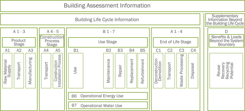
Figure 6.01:
BS EN 15978:2011 – display of modular information for the different stages of the building assessment.
The following explains the practical aspects and scopes of delivering a whole life carbon assessment on a project. This summary goes beyond the British Standard to answer some of the specific questions that arise from undertaking such an assessment in practice.
Boundaries
The assessment should cover all works relating to the proposed building and its intended use, including its foundations, external works within the site, and all adjacent land associated with its typical operations. A planning ‘red line’ can serve as the boundary if applicable. As a minimum, an assessment should be undertaken both at design stage, ie ‘as designed’, and post practical completion, ie ‘as built’. Ideally an assessment should also be undertaken at tender stage to identify design stage carbon reductions and provide an up-to-date ‘carbon budget’ for the main contractor. Further localised assessments can be made to examine, for example, structural or cladding options during the design stages.
Physical characteristics
All items within the project’s cost plan/bill of quantities should be assessed. This would include the building components listed in table 6.01 on page 102.
Reasonable assumptions should be made for provisional sums, and the assessment should cover at least 90% of the cost of each building element category to accommodate the cost efficiency of the assessment.
Reference study period
For all building types an assessment should be 60 years although for shorter life expectancies the anticipated life expectancy can be used. For Infrastructure the period should be 100 years, although for shorter life expectancies the anticipated life expectancy can be used.
Life cycle stages
The WLC assessment should consider all emissions produced over the entire life of the building per the above periods (cradle to grave). Resource efficiency and carbon footprint optimisation also require taking into account future reusability/recyclability of the different elements that make up the building (cradle to cradle). Therefore, all life cycle stages defined by BS EN 15978 (A1-A5, B1-B7, C1-C4, D) should be included in WLC studies.
Floor area measurement
This should be in accordance with Royal Institute of Chartered Surveyors (RICS) property measurement standards (2015 onwards).11 The recommended floor areas sources are listed in order of preference: 1) cost plan/bill of quantities; 2) schedule of accommodation/architectural drawings; 3) BIM model; 4) other.

Quantities measurement
Material quantities should be as per the project cost plan/bill of quantities, BIM model or as estimated from drawings. These should be in accordance with the RICS property measurement standards (2015) and the BCIS elemental standard form of cost analysis.12
Units of measurement to be reported
The unit for reporting the global warming potential/whole life carbon should be kgCO2e or suitable multiples thereof, eg tCO2e. The carbon results should also be normalised in line with the project type, ie kgCO2e/m2 GIA for most building categories, kgCO2e/m3 of internal building volume for storage and industrial units, etc.
Embodied carbon data sources
BS EN 15978 mandates that, ‘Environmental information for the product stage is defined in the product EPD (EN 15804). If EPD unavailable, cradle-to-gate figures to be used calculated according to EN 15804.’ There are several reliable data sources that are acceptable, such as Ecoinvent v3 onwards13 and GaBi vXIV onwards.14 These will help produce an ‘embodied carbon factor’ to be used for each material or component. As far as carbon conversion factors for fuel, refrigerants and water are concerned, the coefficients as issued by the government (BEIS) should be used.15
Table 6.01 represents the context for any assessment. The following sections address the modules/life stages as determined within BS EN 15978.
Modules A1-A3: product stage
The product stage carbon of the different elements should be calculated by assigning the respective suitable embodied carbon factors derived from the acceptable data sources identified in the table. The calculation is: kgCO2e [A1-A3] = material quantity x material embodied carbon factor.
Module A4: transport emissions (factory gate to site)
This is a question of identifying the transport types and the associated attributable emissions for delivery to site. These should be updated at the ‘as built’ stage to paint a more accurate picture, and therefore the contractor should be logging vehicle movements. The calculation is: kgCO2e [A4] = material/system mass x transport distance x carbon conversion factor for fuel use.
Module A5: construction/installation emissions
The carbon emissions from all onsite activities and plant accommodation should be covered. The average figure for construction site emissions of 1400kgCO2e/£100k of project value, as provided by the relevant BRE SMARTWaste tool KPI (2015),16 is suggested as a default for the ‘as designed’ stage. Appropriate allowances for site waste should be made. The site waste rates for different materials should be determined based on the standard wastage rates provided by the WRAP Net Waste tool at the ‘as designed’ stage.17 At the ‘as built’ stage, both rates should be replaced with specific evidence-based site monitoring data provided by the contractor.
Module B: use stage
This stage should capture the carbon emissions associated with any building-related activities over the entire life cycle of the project, from practical completion to demolition. The intention is to measure and highlight to the design team the carbon impacts of design stage decisions post practical completion. Taking future uncertainty into account, sensible scenarios should be developed for the maintenance, repair, replacement, refurbishment and operation of the building. A life cycle analysis (LCA) is therefore an essential requirement.
Module B1: use stage emissions
This covers the release of GHGs from products and materials (eg refrigerants, paints, carpets) during the normal operation of the building. This type of data can be difficult to acquire, but can be accessed from product manufacturers, Health Performance Declaration certificates, EPDs or DEFRA.18
Module B2: maintenance emissions
The carbon emissions of all maintenance activities, including cleaning, should be taken into account. This includes impacts from associated energy and water use. Data for this can be sourced from facilities management/maintenance strategy reports, facade access and maintenance strategy, life cycle cost reports, O&M manuals and professional guidance, eg CIBSE Guide M.19
Modules B3-B4: repair and replacement emissions
This stage involves any emissions arising from the repair and replacement of relevant building components in line with sensible repair and replacement scenarios based on lifespan and further data from facilities management/maintenance strategy reports, facade access and maintenance strategy, life cycle cost reports, O&M manuals and professional guidance. The replacement emissions should capture all emissions associated with the supply of new products [A1-A5]. It should be noted that, for the purposes of consistency, it is assumed that repair, replacement and refurbishment use like-for-like replacements. An allowance should be made for future UK grid decarbonisation. While this is speculative, it does reflect a degree of future transition to a less carbon-intensive energy supply. See National Grid’s Future Energy Scenarios.20
Module B5: refurbishment emissions
BS EN 15978 specifies that, ‘Scenarios for refurbishment of the building, building elements and/or technical equipment shall be developed where details of planned refurbishment are known to the assessor. If no requirements for refurbishment are stated in the client’s brief, the scenarios for refurbishment shall be typical for the type of building being assessed. The scenario for refurbishment shall describe all activities with environmental impacts and aspects arising from the refurbishment process.’ The detailed life cycle analysis should assist with determining the likely refurbishment scenarios.
Module B6: operational energy use
All operational emissions from building-related systems should be included. This covers regulated energy consumption as per Part L (including heating, cooling, ventilation, domestic hot water, lighting and auxiliary systems) as projected throughout the life cycle of the project (excluding maintenance, repair, replacement and refurbishment). It should also include building integrated systems such as lift machinery, security systems, etc. All energy generating units such as solar thermal panels, wind turbines, gas boilers, Combined heat and power (CHP) and heat pumps should be included within the calculation. Data for this section is usually provided by the MEP consultants. Regulated energy use (as per Part L) is usually reported separately from unregulated energy use. It should be noted that the design stage modelled figures can vary from the actual ‘in use’ figures – hence the performance gap.
Module B7: operational water use
All carbon emissions relating to operational water consumption, both supply and waste, throughout the building’s life cycle should be included. At the ‘as designed’ stage of the WLC assessment, estimates for water consumption should be based on the values provided in table 22 of the BSRIA’s ‘Rules of Thumb: Guidelines for the building services’ (5th edition) for the respective building type.21 These should be replaced with more accurate figures at the ‘as built’ stage.
Module C: end of life
The aim of this module is to get the design team to consider the selected materials and methods of construction from the perspective of their disposal or potential for reuse. With resource depletion and the circular economy coming to the fore, we need to understand the extent to which the carbon emissions of this stage can be mitigated by design stage considerations. Projecting into the future is difficult but, for consistency, the basic assumption is that processes will have the same carbon cost as they do today.
Module C1: deconstruction
This module includes all emissions associated with dismantling the building at the end of its life. A practical approach is to consider the overall construction emissions (A5) and treat the deconstruction as a percentage of this figure: a reasonable assumption could be 50%.
Module C2: transport
This refers to transport emissions arising from removing rubble from the building site and taking it to the disposal site. The guidance here is to research disposal sites nearest to the site and average the distance of the closest two. Then, as with A4, kgCO2e [C2] = material/system mass × transport distance × carbon conversion factor for fuel use.
Module C3: waste processing
Module C3 is directly linked to module D, and represents the carbon emissions costs of preparing materials for repurposing (reuse or recycling). C3 represents the carbon cost to bring the materials to the ‘out-of-waste’ state, whereas D represents the benefit. For example, removing mortar from a brick would be covered under C3 while the benefit of the brick reuse would be shown under D.
Module C4: disposal
This includes any emissions arising from landfilling or incinerating building components.
Module D: reuse, recovery, recycling stage
This module is described in BS EN 15978 as, ‘Supplementary information beyond the building life cycle’. However, as noted above, with these issues coming to the fore through circular economic considerations, module D will be increasingly important in WLC assessments. Whereas modules A, B and C represent carbon costs over the life cycle of a building, module D represents future opportunities or benefits. If a material or system has the capacity for beneficial reuse, then this carbon credit can be captured within module D. The difficulty is that delivery is impossible to verify in advance. Nevertheless, designers need to be incentivised to deliver buildings that have a low carbon potential future when dismantled. This benefit, or offset, should be reported separately, as indicated by BS EN 15978. If a product such as brick is only capable of reuse as hardcore, then it can only be valued as such.
Compatibility with BREEAM
BREEAM 201422 includes ‘introductory’ elements (Mat 01 Life cycle impacts; Mat 04 Insulation; Mat 05 Durability and resilience; Ene 01 Reduction of energy use and carbon emissions; Wst 01 Construction waste management; Wst 02 Recycled aggregates) that are relevant to the whole life approach as per BS EN 15978. It is anticipated that the next iteration of BREEAM (2018) will cover embodied and whole life carbon reporting more thoroughly (see Introduction).
Life cycle analysis (LCA)
A life cycle analysis examines, at the design stage, a building’s anticipated fabric and energy performance over its projected lifespan.
A detailed description of LCA can be found in:
- ISO 14040:2006 – LCA Principles and Framework
- ISO 14044:2006 – LCA Requirements and Guidelines
For the built environment an LCA can, as per the above ISOs, be summarised as a systematic set of procedures for compiling and examining the inputs and outputs of materials and energy, and the associated environmental impacts directly attributable to the functioning of a building throughout its life cycle.
For building designers this means developing, over all RIBA stages, an understanding of the impacts of their design decisions over the expected life of a building. The objectives are to optimise the efficient use of resources and minimise the environmental impacts of the building both during construction and throughout its life.
LCA is fundamental to a whole life carbon assessment. Understanding what happens to a building after practical completion is essential to designing low embodied carbon buildings. Design, as previously noted, should account for this from the outset. As a rough guide for large commercial buildings, the embodied carbon emissions over a 60-year period can be similar to those for constructing the building. The following LCAs illustrate key points.
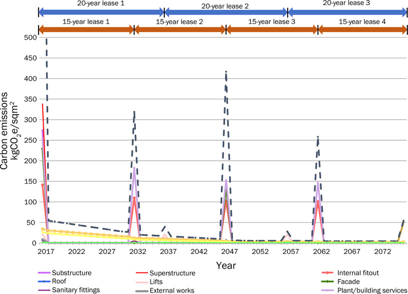
Figure 6.02:
Carbon LCA of an office building showing replacement cycles aligned to 15-year lease cycles.
Figure 6.02 represents a planned LCA for an office building, showing when replacements are expected in line with a 15-year lease cycle (see case study 13 for a more realistic owner-occupier LCA). The horizontal axis is the passage of time; the vertical axis is the annual carbon cost for each of the categories shown. Along the top of the graph are the lease cycle options: 15 or 20 years.
This particular analysis has shown key replacements occurring consistent with a 15-year lease cycle. Life is seldom this tidy; however, what this shows is that the cladding, for example, is expected to be replaced at either 30 or 45 years. Double-glazed units tend to last around 35–40 years, which means that the best moment to replace the cladding from a carbon efficiency point of view would be between two lease events. More realistically, it will either be replaced earlier or possibly later than necessary. Both replacement options would be inefficient in material terms: the first because the cladding is being disposed of before the end of its useful life; the second because the system will start to fail past its expected life, meaning additional operational and maintenance carbon and financial costs. This graph also shows a neat correlation in the replacement of major items such as cladding, central plant roofs, etc. This will almost certainly prove to be optimistic.
An example of where LCAs could have helped understand future impacts is with many recent public buildings. These are often designed using office-type cladding systems, which have relatively short lifespans (40–50 years), and will result in high costs to the local authority when they need replacing. A proper initial LCA, projected over 60–100 years (a not unreasonable period for a public theatre or town hall) would ensure designers think long-term about the economic and social consequences of their choices. (See Chapter 2 on low carbon design choices and the Library of Birmingham.)
The next two graphs show the 15-year interior fitout life cycles of two different types of organisation, both within very large buildings. The first is an international bank; the second is a large technology company. Both LCAs are designed to inform interior fitout choices so as to minimise carbon emissions and optimise efficiency while responding to different corporate cultures. The LCAs start similarly but evolve very differently: the requirement for the bank is to minimise disruption, whereas constant change and reinvention is fundamental to the technology company’s culture.
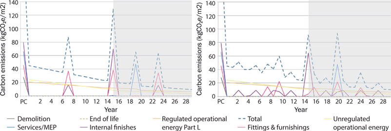
Figure 6.03:
15-year life cycle – interior fitout of an international bank v a large internet company.
What this shows is that there is no one answer to a low carbon requirement and, importantly, what needs to happen after practical completion. The occupiers’ culture should inform the choices made at design stage.
Carbon and financial performance analysis
The carbon cost of component and system choices should be an important determining factor when designing a building. Most building owners, however, make decisions primarily based on financial cost. At SCP, we use two similar (but not to be confused) methods of assessing carbon cost v financial performance: MAC curves and carbon cost analysis.
MAC curves
Marginal abatement cost curves are otherwise known as MAC curves, or MACC. SCP uses these to compare the annualised relative operational carbon performance against the relative financial performance of disparate elements, such as double glazing, draught strips and mechanical controls. Such direct performance comparisons enable us to achieve the optimum operational/financial combination.

Figure 6.04:
An example MACC analysis. Each rectangle represents the carbon benefit and the financial cost/benefit of different elements of construction that affect environmental performance.
MAC curves are a visual method of ranking carbon reduction elements based on the amount of CO2 they save against their cost per tonne of CO2 saved. All those items that impact on environmental performance are shown so that they can be individually and collectively evaluated. The marginal abatement cost is plotted on the y-axis and the elements are ranked against this metric from lowest to highest. The width of the column is equal to the amount of carbon saved by the project, and the area of each column equal to the cost or benefit to the project. Items that are below the line are cost-efficient; items above the line are not.
Carbon cost analysis
SCP has developed a slightly different whole life carbon/cost (CC) tool. A CC analysis enables us to make comparisons between different design options on both financial and carbon cost terms over time. It takes into consideration both the initial construction carbon and financial costs of an element as well as the life cycle impacts of using it within the building fabric. For elements of construction such as cladding or fancoil units, the operational performance can be included. For these and similar examples, the comparison is between a combined embodied/operational carbon performance and a combined financial performance over the anticipated lifespan. Initial selections can then be made from a holistic, ie whole life, perspective on both financial and carbon terms.
This is obviously the most resource-efficient way to assess the design, assembly, use, and disposal of components. However, the costs of creating a building and the costs of its subsequent use are almost always seen as entirely separate. This may be understandable for developers, but it doesn’t make sense for organisations that have a direct interest in the overall lifetime efficiency of a building (eg universities, airports, public buildings, etc). Yet such organisations still work to the ‘lowest cost at practical completion’ model, whatever the long-term implications, and the incentive for project managers is to deliver for lowest initial cost. Overall lifetime resource efficiency and a more circular approach will not be possible until there is a significant change in incentives and therefore culture.
Figure 6.05 is a simple CC analysis showing a comparison between five partition systems against an assumed baseline of plasterboard and metal stud. The analysis compares the supply and assembly of each system, and its use over a 15-year period. Plasterboard and stud is the zero point on both x and y axes. The horizontal dimension of each rectangle represents the carbon variation against the baseline, ie plasterboard and stud; the vertical dimension represents the financial cost or benefit. Both CO2 and financial costs are assessed over this 15-year period, allowing for deterioration and a degree of replacement.
Carbon/cost analysis

Figure 6.05:
Carbon/cost analysis. This compares the carbon and cost performance of design options against a baseline. In this case various partition systems against plasterboard and stud.
- Items A and B show positive carbon and financial performance, with B better in carbon terms and A better financially. Both are a clear improvement on plasterboard and stud.
- Item C is a good carbon performer, but is just below the line financially. This may be worth a second look if the supplier can be persuaded to enhance the financial performance through cheaper units and/or through greater durability. Improved durability will reduce the repair/replacement occurrences and will therefore likely improve both carbon and cost performance.
- Item D is the second cheapest overall, but is the worst carbon performer.
- Item E is poor all around.
Conclusions
Using LCAs, MACC and CC analyses gives building designers a more sophisticated understanding of how their buildings will perform over their lifetime in terms of all CO2e impacts. It is possible to compare not only between options but also between variants within an option, thus getting both a CO2e and a financial understanding of the impacts of recycled content, procurement distances, relative durability, ease of demountability and different end of life scenarios.
Experience shows that LCAs, MACC and CC analyses go a long way to ‘selling’ environmentally-led design over and above the usual feel-good factors. Certainly, project managers and finance directors better understand low carbon thinking and the circular economy when provided with the hard data derived from these analyses.
Life cycle analysis (LCA)
An LCA is a vital tool for whole life carbon management of a building over its anticipated life. Using an LCA informs design decisions made at the outset, and should be a basic tool for any design team. An LCA may also work in parallel with life cycle costing (LCC), which looks at the future cash flow of operating the building post completion.
This simple, user-friendly example LCA looks at the relative impacts of different parts of a building over 100 years. The building in question is an 80,000m2 office scheme for an owner-occupier. The first LCA (shown in figure 6.06) is based on information from the design team at RIBA stage 3. The red diamonds show anticipated replacement cycles of the main components. This indicates a pretty chaotic future for the owner-occupier: after about 20 years, major work to the building is potentially required in a random sequence, meaning significant and uncoordinated replacement events. This is inefficient in both carbon and financial terms. Ideally these events would be grouped to allow for simultaneous replacements of major systems (lifts, plant/services, cladding), thereby minimising disruption.
The design team can use this information to develop a more carefully planned and less wasteful future life for the building. Through material and system specification choices, it is possible to adjust the timing of these events to produce a more synchronised future life cycle. By adopting circular economy thinking, it is also possible to plan for reuse and repurposing of elements that need replacing.
The dilemma for clients is that the aim should be for overall lifetime carbon and financial optimisation rather than focusing only on practical completion; however, we are all judged on the cost of a building on completion, even if it is not the cheapest lifetime solution.

Figure 6.06:
RIBA Stage 3: Whole life tCO
2
e.
In the diagram above, the carbon cost of each item at practical completion (PC) is shown on the left. The largest item by far is the superstructure, at 47,200tCO2e. The fitout is relatively minor, at 12,000tCO2e. However, the WLC (whole life carbon) column shows that over 100 years the fitout has increased to 132,000tCO2e (not including grid decarbonisation) due to regular retrofits, specified as occurring every ten years. The superstructure remains at 47,200tCO2e as no work to it has been assumed. Therefore, fitout-related decisions made at design stage will have a far greater lifetime impact than the structure.
It is also worth noting the anticipated 105,000tCO2e operational carbon emissions (regulated and unregulated). Over 100 years these represent only 29% of the total carbon emissions. For this building, the regulated emissions as per Part L are about half of the total operational emissions. This means that current legislation is only covering about 15% of this building’s total carbon emissions. Also worth noting is that the initial construction carbon cost is approximately a quarter of the overall 100 years’ carbon cost.
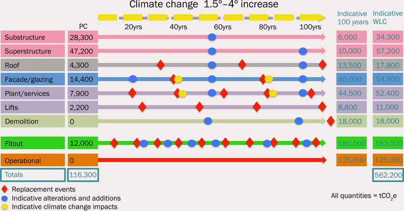
Figure 6.07:
RIBA Stage 3: Whole life tCO
2
e including future change scenario, and predicted climate change.
This next version of the diagram shows the predicted replacement cycles due to wear and tear as before, but includes two additional sets of carbon activities. The blue ovals illustrate changes due to imagined occupier requirements over 100 years, such as extensions, additions and alterations. The yellow ovals show possible impacts of climate change and consequent adaptations to plant/services and cladding. This shows a combination of planned and unplanned scenarios, with indicative figures for this on the right.
This more random mix is exactly what usually happens in the real world. Mapping out speculative future changes to the building helps us to understand the sort of pressures a building will come under in the future and enables a more flexible and responsive approach to the initial design. We may not wish to pay for future climate change today, and of course we don’t know what future technology will be capable of, or what the occupiers will do, but we can at least ensure that these issues are given proper consideration now. We can also ensure that the building does not make future change difficult. This is not a new idea. The Empire State Building (completed in 1931) included in its brief the requirement to enable change by future generations. In 2010 it was refurbished and achieved LEED Gold Standard, something that couldn’t have been predicted in 1931.
Conclusions
LCAs are an invaluable tool to ensure that we design for current and future resource optimisation. It is essential that design teams think proactively about post-practical completion. Key issues are maintenance, future replacement cycles and the impacts of climate change. In a sense, architects and engineers should think of themselves as designing a process rather than a finished building. When it comes to the future, one thing we can be sure of is that pressure on resources will increase; we need to think about this from the outset.