6
CONDITIONAL PROBABILITY

So far, we have dealt only with independent probabilities. Probabilities are independent when the outcome of one event does not affect the outcome of another. For example, flipping heads on a coin doesn’t impact whether or not a die will roll a 6. Calculating probabilities that are independent is much easier than calculating probabilities that aren’t, but independent probabilities often don’t reflect real life. For example, the probability that your alarm doesn’t go off and the probability that you’re late for work are not independent. If your alarm doesn’t go off, you are far more likely to be late for work than you would otherwise be.

In this chapter, you’ll learn how to reason about conditional probabilities, where probabilities are not independent but rather depend on the outcome of particular events. I’ll also introduce you to one of the most important applications of conditional probability: Bayes’ theorem.

Introducing Conditional Probability

In our first example of conditional probabilities, we’ll look at flu vaccines and possible complications of receiving them. When you get a flu vaccine, you’re typically handed a sheet of paper that informs you of the various risks associated with it. One example is an increased incidence of Guillain-Barré syndrome (GBS), a very rare condition that causes the body’s immune system to attack the nervous system, leading to potentially life-threatening complications. According to the Centers for Disease Control and Prevention (CDC), the probability of contracting GBS in a given year is 2 in 100,000. We can represent this probability as follows:

Normally the flu vaccine increases your probability of getting GBS only by a trivial amount. In 2010, however, there was an outbreak of swine flu, and the probability of getting GBS if you received the flu vaccine that year rose to 3/100,000. In this case, the probability of contracting GBS directly depended on whether or not you got the flu vaccine, and thus it is an example of a conditional probability. We express conditional probabilities as P(A | B), or the probability of A given B. Mathematically, we can express the chance of getting GBS as:

We read this expression in English as “The probability of having GBS, given that you got the flu vaccine, is 3 in 100,000.”

Why Conditional Probabilities Are Important

Conditional probabilities are an essential part of statistics because they allow us to demonstrate how information changes our beliefs. In the flu vaccine example, if you don’t know whether or not someone got the vaccine, you can say that their probability of getting GBS is 2/100,000 since this is the probability that any given person picked out of the population would have GBS that year. If the year is 2010 and a person tells you that they got the flu shot, you know that the true probability is 3/100,000. We can also look at this as a ratio of these two probabilities, like so:

So if you had the flu shot in 2010, we have enough information to believe you’re 50 percent more likely to get GBS than a stranger picked at random. Fortunately, on an individual level, the probability of getting GBS is still very low. But if we’re looking at populations as a whole, we would expect 50 percent more people to have GBS in a population of people that had the flu vaccine than in the general population.

There are also other factors that can increase the probability of getting GBS. For example, males and older adults are more likely to have GBS. Using conditional probabilities, we can add all of this information to better estimate the likelihood that an individual gets GBS.

Dependence and the Revised Rules of Probability

As a second example of conditional probabilities, we’ll use color blindness, a vision deficiency that makes it difficult for people to discern certain colors. In the general population, about 4.25 percent of people are color blind. The vast majority of cases of color blindness are genetic. Color blindness is caused by a defective gene in the X chromosome. Because males have only a single X chromosome and females have two, men are about 16 times more likely to suffer adverse effects of a defective X chromosome and therefore to be color blind. So while the rate of color blindness for the entire population is 4.25 percent, it is only 0.5 percent in females but 8 percent in males. For all of our calculations, we’ll be making the simplifying assumption that the male/female split of the population is exactly 50/50. Let’s represent these facts as conditional probabilities:

P(color blind) = 0.0425
P(color blind | female) = 0.005
P(color blind | male) = 0.08

Given this information, if we pick a random person from the population, what’s the probability that they are male and color blind?

In Chapter 3, we learned how we can combine probabilities with AND using the product rule. According to the product rule, we would expect the result of our question to be:

P(male, color blind) = P(male) × P(color blind) = 0.5 × 0.0425 = 0.02125

But a problem arises when we use the product rule with conditional probabilities. The problem becomes clearer if we try to find the probability that a person is female and color blind:

P(female, color blind) = P(female) × P(color blind) = 0.5 × 0.0425 = 0.02125

This can’t be right because the two probabilities are the same! We know that, while the probability of picking a male or a female is the same, if we pick a female, the probability that she is color blind should be much lower than for a male. Our formula should account for the fact that if we pick our person at random, then the probability that they are color blind depends on whether they are male or female. The product rule given in Chapter 3 works only when the probabilities are independent. Being male (or female) and color blind are dependent probabilities.

So the true probability of finding a male who is color blind is the probability of picking a male multiplied by the probability that he is color blind. Mathematically, we can write this as:

P(male, color blind) = P(male) × P(color blind | male) = 0.5 × 0.08 = 0.04

We can generalize this solution to rewrite our product rule as follows:

P(A,B) = P(A) × P(B | A)

This definition works for independent probabilities as well, because for independent probabilities P(B) = P(B | A). This makes intuitive sense when you think about flipping heads and rolling a 6; because P(six) is 1/6 independent of the coin toss, P(six | heads) is also 1/6.

We can also update our definition of the sum rule to account for this fact:

P(A or B) = P(A) + P(B) – P(A) × P(B | A)

Now we can still easily use our rules of probabilistic logic from Part I and handle conditional probabilities.

An important thing to note about conditional probabilities and dependence is that, in practice, knowing how two events are related is often difficult. For example, we might ask about the probability of someone owning a pickup truck and having a work commute of over an hour. While we can come up with plenty of reasons one might be dependent on the other—maybe people with pickup trucks tend to live in more rural areas and commute less—we might not have the data to support this. Assuming that two events are independent (even when they likely aren’t) is a very common practice in statistics. But, as with our example for picking a color blind male, this assumption can sometimes give us very wrong results. While assuming independence is often a practical necessity, never forget how much of an impact dependence can have.

Conditional Probabilities in Reverse and Bayes’ Theorem

One of the most amazing things we can do with conditional probabilities is reversing the condition to calculate the probability of the event we’re conditioning on; that is, we can use P(A | B) to arrive at P(B | A). As an example, say you’re emailing a customer service rep at a company that sells color blindness–correcting glasses. The glasses are a little pricey, and you mention to the rep that you’re worried they might not work. The rep replies, “I’m also color blind, and I have a pair myself—they work really well!”

We want to figure out the probability that this rep is male. However, the rep provides no information except an ID number. So how can we figure out the probability that the rep is male?

We know that P(color blind | male) = 0.08 and that P(color blind | female) = 0.005, but how can we determine P(male | color blind)? Intuitively, we know that it is much more likely that the customer service rep is in fact male, but we need to quantify that to be sure.

Thankfully, we have all the information we need to solve this problem, and we know that we are solving for the probability that someone is male, given that they are color blind:

P(male | color blind) = ?

The heart of Bayesian statistics is data, and right now we have only one piece of data (other than our existing probabilities): we know that the customer support rep is color blind. Our next step is to look at the portion of the total population that is color blind; then, we can figure out what portion of that subset is male.

To help reason about this, let’s add a new variable N, which represents the total population of people. As stated before, we first need to calculate the total subset of the population that is color blind. We know P(color blind), so we can write this part of the equation like so:

Next we need to calculate the number of people who are male and color blind. This is easy to do since we know P(male) and P(color blind | male), and we have our revised product rule. So we can simply multiply this probability by the population:

P(male) × P(color blind | male) × N

So the probability that the customer service rep is male, given that they’re color blind, is:

Our population variable N is on both the top and the bottom of the fraction, so the Ns cancel out:

We can now solve our problem since we know each piece of information:

Given the calculation, we know there is a 94.1 percent chance that the customer service rep is in fact male!

Introducing Bayes’ Theorem

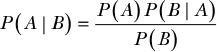
There is nothing actually specific to our case of color blindness in the preceding formula, so we should be able to generalize it to any given A and B probabilities. If we do this, we get the most foundational formula in this book, Bayes’ theorem:

To understand why Bayes’ theorem is so important, let’s look at a general form of this problem. Our beliefs describe the world we know, so when we observe something, its conditional probability represents the likelihood of what we’ve seen given what we believe, or:

P(observed | belief)

For example, suppose you believe in climate change, and therefore you expect that the area where you live will have more droughts than usual over a 10-year period. Your belief is that climate change is taking place, and your observation is the number of droughts in your area; let’s say there were 5 droughts in the last 10 years. Determining how likely it is that you’d see exactly 5 droughts in the past 10 years if there were climate change during that period may be difficult. One way to do this would be to consult an expert in climate science and ask them the probability of droughts given that their model assumes climate change.

At this point, all you’ve done is ask, “What is the probability of what I’ve observed, given that I believe climate change is true?” But what you want is some way to quantify how strongly you believe climate change is really happening, given what you have observed. Bayes’ theorem allows you to reverse P(observed | belief), which you asked the climate scientist for, and solve for the likelihood of your beliefs given what you’ve observed, or:

P(belief | observed)

In this example, Bayes’ theorem allows you to transform your observation of five droughts in a decade into a statement about how strongly you believe in climate change after you have observed these droughts. The only other pieces of information you need are the general probability of 5 droughts in 10 years (which could be estimated with historical data) and your initial certainty of your belief in climate change. And while most people would have a different initial probability for climate change, Bayes’ theorem allows you to quantify exactly how much the data changes any belief.

For example, if the expert says that 5 droughts in 10 years is very likely if we assume that climate change is happening, most people will change their previous beliefs to favor climate change a little, whether they’re skeptical of climate change or they’re Al Gore.

However, suppose that the expert told you that in fact, 5 droughts in 10 years was very unlikely given your assumption that climate change is happening. In that case, your prior belief in climate change would weaken slightly given the evidence. The key takeaway here is that Bayes’ theorem ultimately allows evidence to change the strength of our beliefs.

Bayes’ theorem allows us to take our beliefs about the world, combine them with data, and then transform this combination into an estimate of the strength of our beliefs given the evidence we’ve observed. Very often our beliefs are just our initial certainty in an idea; this is the P(A) in Bayes’ theorem. We often debate topics such as whether gun control will reduce violence, whether increased testing increases student performance, or whether public health care will reduce overall health care costs. But we seldom think about how evidence should change our minds or the minds of those we’re debating. Bayes’ theorem allows us to observe evidence about these beliefs and quantify exactly how much this evidence changes our beliefs.

Later in this book, you’ll see how we can compare beliefs as well as cases where data can surprisingly fail to change beliefs (as anyone who has argued with relatives over dinner can attest!).

In the next chapter, we’re going to spend a bit more time with Bayes’ theorem. We’ll derive it once more, but this time with LEGO; that way, we can clearly visualize how it works. We’ll also explore how we can understand Bayes’ theorem in terms of more specifically modeling our existing beliefs and how data changes them.

Wrapping Up

In this chapter, you learned about conditional probabilities, which are any probability of an event that depends on another event. Conditional probabilities are more complicated to work with than independent probabili-ties—we had to update our product rule to account for dependencies—but they lead us to Bayes’ theorem, which is fundamental to understanding how we can use data to update what we believe about the world.

Exercises

Try answering the following questions to see how well you understand conditional probability and Bayes’ theorem. The solutions can be found in Appendix C.

• What piece of information would we need in order to use Bayes’ theorem to determine the probability that someone in 2010 who had GBS also had the flu vaccine that year?
• What is the probability that a random person picked from the population is female and is not color blind?
• What is the probability that a male who received the flu vaccine in 2010 is either color blind or has GBS?