
CHAPTER NINE
File Systems—NTFS and Beyond
CHAPTER 9 FURTHER EXAMINES file systems, focusing now on file systems beyond FAT, which are those most likely to be encountered by the cyber forensic investigator.
As technology truly does march to its own beat and is constantly in a state of flux and change, the cyber forensics professional should be attuned to the changes announced by vendors regarding their operating systems and the file system variations that may emerge from any advancement in operating system designs and future release updates to these operating systems.
Next up, a review of another Windows file system, the New Technology File System (NTFS), whose use started with Windows NT in 1993. Windows XP, 2000, Server 2003, 2008, and Windows 7 also all use later versions of NTFS. The filing system is very complex and to make matters worse there are very little published specifications from Microsoft that describes the “on-disk layout.”
What this means is that logical representations of the physical structure of this file system are speculative and very difficult to visualize. It’s a good thing our goal here is not an in-depth bit-for-bit analysis of each file system, but instead a more conceptual understanding of file systems in general.
An important concept in understanding the NTFS design is that all data is allocated to files, including the file system itself; the file system files can be located anywhere in the volume, as would a regular file. Therefore, NTFS does not have a normal File System Layout like FAT, as discussed in Chapter 8, where there are areas at the beginning of the volume reserved for these data.
The entire file system is considered a data area, and any sector can be allocated to a file. The only constant within the NTFS file structure is that the first sectors contain the boot sector, similar to the volume boot in FAT.
The New Technology File System (NTFS) contains the following “components”:
1. Partition Boot Sector (PBR)—similar to VBR in FAT
2. Master File Table (MFT)—similar to directory entry in FAT
3. $bitmap—similar to the FAT
The Partition Boot Record (PBR) is comprised of 16 sectors, as opposed to one sector with FAT. Typically, however, only eight sectors of the 16 sectors available are used.
Byte offset 0–10 contains jump instructions and the OEM ID (NTFS). OEM is the acronym for Original Equipment Manufacturer, and in NTFS, this is represented by a string of characters that identifies the name and version number of the operating system that formatted the volume.
Figure 9.1 is the first sector of the boot record as seen in a HEX editor. Remember, NTFS allocates the first 16 sectors for the boot “sector.”
FIGURE 9.1 First Sector of the Boot Record (NTFS)
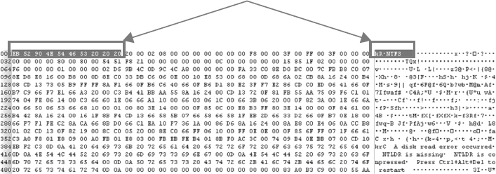
Byte offset 0–9 is highlighted in Figure 9.1, showing the OEM identifier “NTFS.” Byte offset 3–6 in the first sector of the boot sector will contain the ASCII “NTFS” representation of HEX 4E 54 46 53 defining it as such.
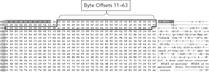
Figure 9.2 displays byte offsets 11–63 containing partition parameter information.
FIGURE 9.2 Byte Offsets 11 through 63 Containing Partition Parameter Information
The reader may wish to review Appendix 8A, Partition Table Fields, for a more in depth look at the data fields and their representation in the PBR.
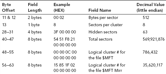
Table 9.1 lists and describes the field name and decimal value for the contents of byte offsets 11 through 63 of the PBR.
TABLE 9.1 Byte Offsets 11 through 63 of the PBR
A further look at the PBR will reveal that byte offset 64–509 contains the boot strap code, and byte offset 510–511, by default, and as a control, contains the end of file marker, with a HEX value of 55AA.
The Master File Table (MFT) is the heart of the NTFS file system. It is analogous to the directory entry in the FAT filing systems; it will contain much of the metadata, similar to the card catalogue in our library analogy. The MFT is much like a database as it contains entries to track all data contained within the file system, and in this sense it acts a bit like the FAT. In our comparisons to FAT, the MFT actually has functionalities similar to both directory entries and the FAT. The MFT contains an entry for every file and directory in the partition, including itself, which is named $MFT.
The MFT is scattered throughout the disk structure; it is not contained or constrained to certain specified sectors as are FAT directory entries. Being that the MFT is not confined to predefined sectors, it allows the file system to be dynamic and expand as necessary. It is not bounded or limited to a certain number of files as with FAT filing systems.
Each entry (or record) does however have a fixed length of 1,024 bytes. Being that there are 512 bytes per sector, there are two sectors per MFT entry.
Determining the Location of the MFT
To determine the MFT’s starting location we look at byte offset 48–55 (eight bytes) in the Boot Record. The decimal value of these binary values gives us the Logical Cluster number for the $MFT.
Figure 9.3 shows the placement of byte offset 48–55, within the PBR, where we would look for the start of the MFT.
FIGURE 9.3 Byte Offset 48 through 55 and the Start of the MFT
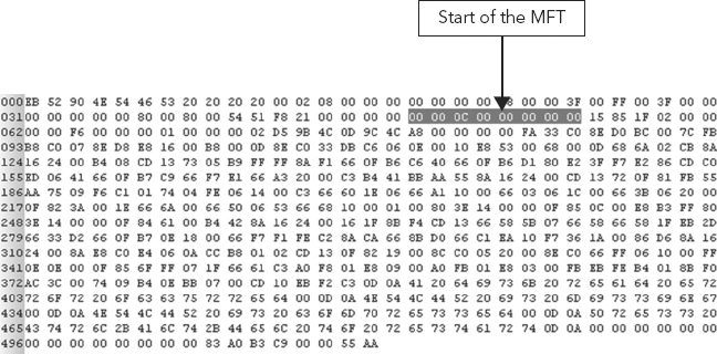
Determining the location of the MFT ($MFT) requires a little bit of computer math and remembering our previous discussions on endianness. To start, we identify the HEX values for byte offset 48–55. By looking at Figure 9.3, we determine that the HEX values for byte offset 48–55 equals HEX 00 00 0C 00 00 00 00 00, which by the way, is in big endian format.
Next, rearrange these HEX values into little endian, resulting in HEX 00 00 00 00 00 C0 00 00.
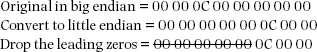
Why are the leading zeros dropped? HEX 00 in decimal equals zero, and just as with any decimal number a zero preceding a number other than zero is usually ignored (e.g., 098 is typically written as simply 98).
Finally, convert the resulting HEX value 0C 00 00 into its decimal equivalent, thereby obtaining a value of 786,432. Thus, confirming the MFT will begin at cluster offset 786,432.
Figure 9.4 shows the first attribute entry in the first sector of the MFT as viewed by a HEX editor.
FIGURE 9.4 First Attribute Entry in the First Sector of the MFT
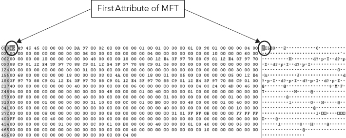
The MFT views everything about the file as an attribute, metadata and data alike. The first byte of the MFT entry is the standard file record header (see Figure 9.4). The first four bytes of the MFT are combined to form the file Identifier, “FILE.” It is this attribute that defines this sector as a record.
In fact, some of the actual data contained within the file will be present within the MFT entry, as it is considered just another attribute. If a file is small, sometimes the entirety of that file is stored within the MFT entry; this is called resident data.
A File and Its Attributes
If the file is too large for all its data to be contained within the MFT then the file is allocated to a cluster. The cluster runs are then stored in place of the resident data. Typically, 480 bytes is the maximum length for resident files.
An attribute has two parts:
1. Header—Identifies the attribute: file type, file size, and name. Also, it has flags to identify if the attribute is compressed or encrypted. Header is generic and standard to all attributes.
2. Content—Actual contents of the file for a resident file. Cluster location of file for nonresident files. Content is specific and unique and can be any size.
All file attributes are stored in one of two different ways, depending on the characteristics of the attribute, especially size:
1. Resident Attributes—Attributes that are stored directly within the file’s primary MFT record itself. Many of the simplest and most common file attributes are stored resident in the MFT file. In fact, some are required by NTFS to be resident in the MFT record for proper operation. For example, the name of the file, and its creation, modification, and access date/time stamps are resident for every file.1
2. Non-Resident Attributes—If an attribute requires more space than is available within the MFT record, it then cannot be stored in that record. Instead, the attribute is placed in a separate location on the disk. A pointer is placed within the MFT that leads to the location of the attribute. This is called non-resident attribute storage.
A letter or package received at the post office can be seen as an analogy. The attribute would be the envelope, box, or storage container. The outside of the container may have your name, address, and possibly the contents written on it. The inside of the box actually contains the contents.2
Thus, all items are stored in containers (boxes or envelopes). Containers may be of all sizes and shapes, all with different contents; however, the data written on the outside of the container all contain the same info—name, address, and contents.
In this analogy the header equates to the outside of the box and the content equates to the contents of the box.3 Readers desiring further information regarding attributes are encouraged to review Appendix 9A, Common NTFS System Defined Attributes.
$Bitmap
Another component of NTFS, which is somewhat similar in functionality to the FAT, is $Bitmap. In comparing NTFS and FAT filing systems it is apparent that the MFT in NTFS actually acts as a directory entry and performs some FAT functionality. As discussed previously, the MFT contains the non-resident attributes that points to where the data is located. This is essentially similar to the role of the FAT.
So what role does $Bitmap perform and how is it similar to the FAT? The $Bitmap is a file that represents cluster allocation within a partition. It identifies if a cluster is allocated or unallocated. Each bit within the $Bitmap represents a cluster. If a bit representing a cluster has a value of zero (in binary), then that cluster is available for use or unallocated; if the bit has a value of one (1), then that cluster is unavailable or allocated.
The $Bitmap does not identify starting locations of files, length of files, cluster size of files, or any data regarding file location or storage. It simply tells the system if the cluster is allocated or unallocated.
Explaining the complexities of NTFS is somewhat simplified when building upon an existing understanding of FAT. Both are similar enough to be somewhat analogous. The point of describing either of these systems is to understand how file systems can work in general. By grasping such file system concepts we begin to understand how one file system (such as NTFS) can be much more dynamic and adaptive to growth than another. We also, and perhaps more importantly to the cyber forensic investigator, begin to understand how data are stored.
Microsoft’s Extended File Allocation Table (exFAT) was released with Windows Vista SP1 (Service Pack One). A file system designed for Flash memory storage and other external devices, ExFAT expands upon the file size, drive size, and directory limitations of older versions of FAT yet maintains the low overhead of FAT.
A robust and complex file system like Windows NTFS allows for relatively efficient storage in extremely large drives. However, the overhead of efficient storage is the consumption of system resources, such as memory and processing power. In systems where resources are limited NTFS is inefficient. The NTFS file system consumes a lot of resources maintaining itself. ExFAT was designed for use in those areas where NTFS is an overkill and inefficient.
There are other filing systems beyond Microsoft’s NTFS, exFAT, and FAT. As can be expected, different Operating Systems utilize different filing systems, and as technology advances so too do the functionalities contained within Operating Systems and therefore with File systems. Many of these filing system concepts do not align themselves to the Microsoft filing system paradigm. Slight similarities do exist, being that the end goal is ultimately the same, namely accessing files, but generally the Microsoft filing system is not a model for all file systems.
ALTERNATIVE FILING SYSTEM CONCEPTS
Alternative file systems and the concepts associated with these alternative file systems will be explored in the remainder of this chapter.
Binary Search Tree Filing System
A binary tree is a hierarchical data structure concept used for placing and locating files. Conceptually, in a hierarchical tree data structure things are ordered above or below other things. The tree is made up of nodes that are linked together as either parents or children.
The top node of the tree is called the root. The nodes directly under another node are referred to as children. The nodes directly above another node are called parents. Nodes with no children are sometimes called leaves. The Order of the binary tree is equal to the maximum number of children per node (two with binary trees). The Depth of the tree is equal to the length of the path (in number of nodes) from the top root node to the lowest leaf. The search tree size is equal to the total number of nodes.
In a basic binary tree each node can have a maximum of only two children. Within a binary tree structure each node (item in the tree) has a distinct value. Both left and right subtrees must also follow binary search tree structure. The left subtree of a node contains only values less than the parent nodes value and the right subtree of a node contains only values greater than the parent nodes value. Again, each node has a maximum of only two children. Figure 9.5 shows a graphical look at a binary tree structure.
FIGURE 9.5 Binary Search Tree Structure
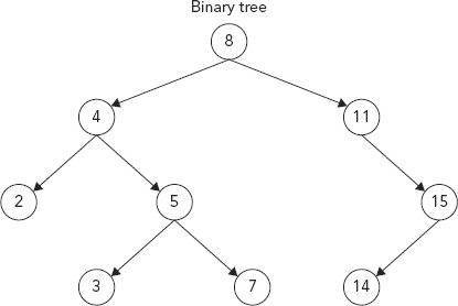
For example, in the image in Figure 9.5, the root node 8 is a parent of node 4 and node 11. And likewise, node 4 and node 11 are children of root node 8. The search tree size is 9 nodes; its depth is 3. The leaves are nodes 2, 3, 7, and 14. The left nodes are 4, 2, and 3, and the right nodes are 5, 7, 11, and 15. All nodes except for node 8 are children. Figure 9.6 shows the relationship between the root, parent, and leaves.
FIGURE 9.6 Binary Tree Relationships
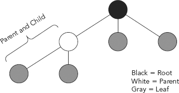
The binary tree (b-tree) is a useful data structure for rapidly storing sorted data and rapidly retrieving stored data. It is the relationship between the children and the parent node which makes the binary tree such an efficient data structure. It is the leaf on the left that has a lesser key value, and it is the leaf on the right that has an equal or greater key value. As a result, the leaves on the farthest left of the tree have the lowest values, whereas the leaves on the right of the tree have the greatest values. More importantly, as each parent node branches to two other leaves (e.g., children), a new, smaller subset within the binary tree is created. Due to this subdividing process, it is possible to easily access and insert data in a binary tree using search and insert functions recursively called on successive leaves.
The advantage of a binary tree (and variants of b-trees) has to do with disk read efficiencies, the speed of locating and presenting data. As data is called for, records need to be searched in order to locate the data. Searching records takes time. In FAT and NTFS this search can take a lot time (relatively speaking) as the OS searches through what can be the entirety of the file system.
Data in a binary search tree are stored in tree nodes, and must have associated with them an ordinal value or key; these keys are used to structure the tree such that the value of a left child node is less than that of the parent node, and the value of a right child node is greater than that of the parent node. Sometimes, the key and datum are one and the same. Typical key values include simple integers or strings, the actual data for the key will depend on the application.
To perform a search, first start at the root of the tree, and compare the ordinal value of the root to the ordinal value of the node to be located. If the ordinal value is less than the root, follow the left branch of the root, or else follow the right branch. Start the comparison again, but at the branch compare the ordinal value of the child with the node to be located. Traversal of the tree continues in this manner until identifying the node.4
The hierarchical index structure of the binary tree allows the search to skip either right or left subtree records at each level. As the search descends the tree, the volume of data needing to be read is quickly reduced.
For the sake of argument say each division within the tree was split 50/50; 50 percent of the records on the left side and 50 percent on the right side. As the search would descend the tree the amount of potential records needing to be searched would drop by half at each layer. The hierarchical index minimizes the number of disk reads necessary to locate a particular record.
To further illustrate this point, assume that the target value of a search is contained within a data set of fictional characters, with the target value identified as Holmes, Sherlock. In this example, the data set will be searched alphabetically, with the objective of identifying the individual record for Holmes, Sherlock (see Figure 9.7).
FIGURE 9.7 Fictional Character Name Data Set
First begin by selecting the middle element of the data set (Figure 9.8), essentially the median, and comparing it against the target value. If the values match it will return success.
FIGURE 9.8 Middle Element of the Data Set
In this example the median value of “M” does not match the “H” of Holmes. If the target value (our example “H”) is higher than the value of the median (“M”) it will take the upper half of the data set and perform the same operation against it.
Likewise, if the target value is lower than the median value (“M”) it will perform the operation against the lower half. (See Figure 9.9.)
FIGURE 9.9 Target Value (“H”) Is Higher than the Value of the Median (“M”)
Given that the target value (our example “H”) is higher than the value of the median (“M”), the search will probe the upper half of the data set. The data set is again split at the median, and the target value (“H”) is again compared to the newly established median (which in this second iteration is now, “F”). (See Figure 9.10.)
FIGURE 9.10 Second Iteration Upper Half of Data Set to Be Probed
Given that the target value (“H”) is not higher than the value of the median (“F”), the search will not probe the upper half of the data set (A, B, C, D, E,) but rather the lower half of the remaining date set (G, H, I, J, K, L). (See Figure 9.11.)
FIGURE 9.11 Lower Half of Data Set to Be Probed
Given that the target value (“H”) is now higher than the value of the next median value (“I”), the search will probe the upper half of the data set (G, H, I) rather than the lower half of the remaining date set (J, K, L). (See Figure 9.12.)
FIGURE 9.12 Binary Search Third Iteration
The binary search process will continue to halve the data set with each iteration, until the value has been found or until it can no longer split the data set. With the fourth iteration the target value “H” is found (see Figure 9.13) and the initial search process terminates.
FIGURE 9.13 Binary Search Fourth Iteration
The same search methodology will begin anew as the data set “H” is probed for an exact match to the target value “Holmes.”
B-Tree
A b-tree is conceptually similar to a binary tree in that they are both methods of placing and locating files, but the two are not analogous. The main difference is b-trees are of a higher order, meaning nodes can have more than two children. This allows for a record to be found by passing through fewer nodes (the depth of the tree would be less) than if there were only two children per node. The higher order within a b-tree therefore minimizes the number of times a medium or (nodes) must be accessed to locate a desired record. In other words, less writes to the disk speeds up the search process.
Each piece of data stored in a b-tree is called a “key” because each key is unique and can occur in the b-tree in only one location.
A b-tree consists of “node” records containing the keys, and pointers that link the nodes of the b-tree together. Every b-tree is of some “order n,” meaning nodes contain from n to 2n keys, and nodes are thereby always at least half full of keys. Keys are kept in sorted order within each node. Corresponding lists of pointers are effectively interspersed between keys to indicate where to search for a key if it isn’t in the current node. A node containing k keys always contains k + 1 pointers.
For example, Figure 9.14 shows a portion of a b-tree with order 2 (nodes have at least two keys and three pointers). Nodes are delimited with ellipses. The keys are city names, and are kept sorted alphabetically in each node. On either side of every key are pointers linking the key to subsequent nodes.
FIGURE 9.14 Portion of a B-Tree with Order 2 (nodes have at least two keys and three pointers)
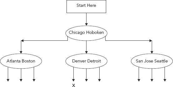
To find the key “Des Moines,” we begin searching at the top “root” node. “Des Moines” is not in the node but sorts between “Chicago” and “Hoboken,” so we follow the middle pointer to the next node. Again, “Des Moines” sorts between “Denver” and “Detroit” so we follow that node’s first pointer down to the next node (marked with an “X”).
Eventually, we will either locate the key, or encounter a “leaf” node at the bottom level of the b-tree with no pointers to any lower nodes and without the key we want, indicating the key is nowhere in the b-tree.
Searching a b-tree for a key always begins at the root node and follows pointers from node to node until either the key is located or the search fails because a leaf node is reached and there are no more pointers to follow.
Even very large b-trees can guarantee only a small number of nodes must be retrieved to find a given key. For example, a b-tree of 10,000,000 keys with 50 keys per node never needs to retrieve more than four nodes to find any key.5
The maximum number of children per node is the order of the tree; b-trees are also binary and therefore can have an order of 32, 64, 128, or more (children per node).
In a tree, the records (data) are stored in locations called leaves. There can be billions of records (leaves). Depth changes as records increase to insure that the b-tree functions optimally for the number of records it contains.
Hierarchical File System
Hierarchical File System (HFS) is the file system used in Apple Macintosh systems. It was introduced by Apple in 1995, replacing their legacy MFS (Macintosh Filing System). Files are referenced with unique file IDs rather than file names; these unique identifiers can be 255 characters long. It uses a b-tree structure, which is a variance of the b-tree file system. As described above, it is this tree data structure that keeps data sorted and allows for quick searches, insertions, and deletions.
UNIX File System
UNIX File System (UFS) is the file system used by the UNIX Operating System, also called Berkeley File System Composition. There is what is called a “Superblock,” which contains a “magic number” identifying this as a UFS file system (see Chapter 4 and Appendix 4C for additional information on magic numbers), as well as information describing geometry, statistics, and parameters of drive; functionally, it is similar to Volume Boot Record, which we have detailed in FAT filing systems.
UFS also contains what are called Inodes, which contain file attributes (i.e., metadata) that are functionally similar to directory entries. These Inodes are contained within groups called Cylinder Groups along with Data Blocks, which contain the actual data.
EXT2 and EXT3
EXT are file systems used in many Linux Operating Systems. Linux supports many file systems but EXT is the default file system of most distributions. EXT3 is a newer version of EXT2; EXT3 adds file system journaling; however, basic construction is the same.
EXT is based on the UFS File System but, as is the case with most things Linux, much of the complexities of UFS were removed, keeping this file system relatively simple. This filing system splits disk space into Block Groups (similar to Cylinder Groups of UFS). The block group sections all contain the same number of blocks, except for the last one, which may contain less depending upon drive size. These blocks are used to store file names, metadata, and file content.
EXT stores all the data relating to a file, unlike FAT or NTFS, which stores metadata in separate locations.
A workable analogy for this filing system would be the theater. The seats in a theater are grouped into sections, just as blocks on a hard drive are grouped into Block Groups. Each section of the theater (block group) is numbered and each section contains the same amount of seats (blocks).
Only the basic layout information of EXT is stored in what is called a Superblock data structure, again comparable to the Volume Boot in FAT. The file content is stored in the blocks, which are groups of consecutive sectors. Blocks in their use here are comparable to clusters. Similar to UFS, the metadata for each file and directory is also stored in the block in a data structure called an inode. The inode has a fixed size and is located within an inode table. There is one inode table per block group.
Various filing systems and their components may have different names and their physical placement on the drive may vary, but functionally all file systems require similar pieces: those that identify it, those that identify its data, and those that contain the data itself.
We addressed file systems here to explain these components and how data is accessed, stored, deleted, and so on. For the purposes of this text we did not cover each and every file system that a cyber forensics investigator may encounter, nor did we provide the exact bit-for-bit break down of each and every file system—for a good reason.
Books have been written and continue to be written about each of these filing systems and filing system concepts. Existing file systems will evolve and new file systems will develop; we will continue to see this growth in cell phones, iPhones, PDAs, iPads, storage media, and all the new devices to come. What is important for the reader is that by having read this chapter, you now have a better understanding, more confidence, and a greater appreciation of the concepts of file systems and the function they perform.
Technology will continue to evolve, and so must the cyber forensics investigator. As the investigator, you will, in some cases, find yourself potentially drawn to specializing in a certain system type (e.g., Windows, Unix, etc.). As this occurs you will find yourself proficient in one file system type over another. This is the natural evolution of learning and mastering. Within the cyber forensics field, and computers in general, it is next to impossible for a single person to know everything.
Within cyber forensics you will come across investigators with specializations such as the cell phone maharishi, the MAC guru, or the RAID go-to person.
Be confident, you’re now one step closer to being the “file systems” guru!
1. Charles M. Kozierok, NTFS File Attributes (April 2001), www.pcguide.com/ref/hdd/file/ntfs/filesAttr-c.html.
2. Ibid.
3. Carrier, B., File Systems Forensic Analysis (Upper Saddle River, NJ: Pearson Education, 2005).
4. H. Sauro (August 18, 2008), “A simple Binary Search Tree written in C#,” www.codeproject.com/KB/recipes/BinarySearchTree.aspx, retrieved December 2010.
5. “B-tree algorithms,” Semaphore Corporation, 484 Washington St Ste B PMB 344, Monterey CA 93940-3052, www.semaphorecorp.com/btp/algo.html, used with permission, retrieved December 2010.
APPENDIX 9A: COMMON NTFS SYSTEM DEFINED ATTRIBUTESa
Here’s a list of the most common NTFS system-defined attributes:
Standard Information (SI): Contains “standard information” for all files and directories. This includes fundamental properties such as date/timestamps for when the file was created, modified, and accessed. It also contains the “standard” FAT-like attributes usually associated with a file (such as if the file is read-only, hidden, and so on).
Attribute List: This is a “meta-attribute”: an attribute that describes other attributes. If it is necessary for an attribute to be made non-resident, this attribute is placed in the original MFT record to act as a pointer to the non-resident attribute.
File Name (FN): This attribute stores a name associated with a file or directory. Note that a file or directory can have multiple file name attributes, to allow the storage of the “regular” name of the file, along with an MS-DOS short filename alias. Stores name in Unicode.
Security Descriptor (SD): The access control and security properties of the file.
Volume Name, Volume Information, and Volume Version: These three attributes store key name, version, and other information about the NTFS volume. Used by the $Volume metadata file.
Data: Contains file data. By default, all the data in a file is stored in a single data attribute—even if that attribute is broken into many pieces due to size, it is still one attribute.
Index Root Attribute: This attribute contains the actual index of files contained within a directory, or part of the index if it is large. If the directory is small, the entire index will fit within this attribute in the MFT; if it is too large, some of the information is here and the rest is stored in external index buffer attributes.
Index Allocation Attribute: If a directory index is too large to fit in the index root attribute, the MFT record for the directory will contain an index allocation attribute, which contains pointers to index buffer entries containing the rest of the directory’s index information.
Bitmap: Contains the cluster allocation bitmap. Used by the $Bitmap metadata file.
- Similar in function to FAT tables in FAT.
- Contains one bit for each cluster in the partition. Unlike FAT, it tracks cluster allocation only. It does not track cluster runs. If a bit (representing a cluster) has a 1, the cluster is allocated to a file. If the bit (representing a cluster) has a 0, the cluster is unallocated, or available for use. Very simple.
Extended Attribute (EA) and Extended Attribute Information: These are special attributes that are implemented for compatibility with OS/2 use of NTFS partitions.
Most file systems exist to read and write file content, but NTFS exists to read and write attributes, which can contain file content or header (metadata) content. It’s as if NTFS did not differentiate between metadata and regular data (file contents).
Box Analogy
Think about an attribute as a box or storage container. The outside of the container may have your name, address, and contents written on it; the inside is the contents.
The header is generic and standard to all attributes, while the content is a specific type of attribute and can be any size.
Thus, all items are stored in “boxes.” Boxes may be of all sizes and shapes with different contents, but the outside all contain the same info: name, address, and contents.
So the header equates to the outside of the box and the content equates to the contents of the box.
a Kozierok, C. (Site Version: 2.2.0 – Version Date: April 17, 2001), “NTFS File Attributes,” www.pcguide.com/ref/hdd/file/ntfs/filesAttr-c.html, retrieved November 2011.