Chapter 1
Radio Wave Fundamentals
Radio wave propagation is governed by the theory of electromagnetism laid down by the Scottish physicist and mathematician James Clerk Maxwell (13 June 1831 to 5 November 1879) who demonstrated that electricity, magnetism and light are all manifestations of the same phenomenon. Electromagnetic wave propagation depends on the properties of the transmission medium in which they travel. Classifications of transmission media include linear versus nonlinear, bounded versus unbounded, homogeneous versus nonhomogeneous and isotropic versus nonisotropic. Linearity implies that the principle of superposition can be applied at a particular point, whereas a medium can be considered bounded if it is finite in extent or unbounded otherwise. Homogeneity refers to the uniformity of the physical properties of the medium at different points and an isotropic medium has the same physical properties in different directions.
In this chapter we start by a revision of the fundamentals of Maxwell's wave equations and polarization. This is followed by a discussion of the different propagation phenomena including reflection, refraction, scattering, diffraction, ducting and frequency dispersion. These are discussed in relation to different transmission media such as propagation in free space, the troposphere and the ionosphere. For a more detailed treatment of the subject, the reader is referred to [1, 2].
1.1 Maxwell's Equations
Originally Maxwell's equations referred to a set of eight equations published by Maxwell in 1865. In 1884 Oliver Heaviside, concurrently with other work by Willard Gibbs and Heinrich Hertz, modified four of these equations, which were grouped together and are nowadays referred to as Maxwell's equations. Individually, these four equations are known as Gauss's law, Gauss's law for magnetism, Faraday's law of induction and Ampere's law with Maxwell's correction.
Fundamental to Maxwell's four field equations is the differential vector operator ![]() (pronounced del) and the bold denotes a vector given by:
(pronounced del) and the bold denotes a vector given by:
1.1 ![]()
For a scalar V and a vector function A with components along the xyz axes:
1.2 ![]()
there are three possible operations related to the ![]() operator, defined as follows:
operator, defined as follows:
1.3 ![]()
1.4 ![]()
1.5 ![]()
1.6 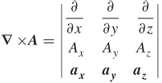
Related to these operators are the following identities:
1.7 ![]()
1.8 ![]()
1.9 ![]()
where
![]()
Using the ![]() operator, Maxwell's four equations relate the electric field E volts per m (V/m) and magnetic field H amperes per metre (A/m), as given in Equations (1.11 to 1.14):
operator, Maxwell's four equations relate the electric field E volts per m (V/m) and magnetic field H amperes per metre (A/m), as given in Equations (1.11 to 1.14):
1.12 ![]()
where ρ is the charge density in coulombs per cubic metre (C/m3), ![]() is the permittivity in farads per metre (F/m), μ is the permeability in henrys per metre (H/m) and σ is the conductivity of the medium in mho per metre or siemens per metre (S/m), which is assumed to be homogenous, isotropic and source-free. The permittivity and permeability of the medium are usually expressed relative to vacuum as
is the permittivity in farads per metre (F/m), μ is the permeability in henrys per metre (H/m) and σ is the conductivity of the medium in mho per metre or siemens per metre (S/m), which is assumed to be homogenous, isotropic and source-free. The permittivity and permeability of the medium are usually expressed relative to vacuum as ![]() and
and ![]() and are given by:
and are given by:
1.15b ![]()
Note that, in general, the permittivity in Equation (1.15a) is complex but in many representations the imaginary part is not included. Maxwell's equations can also be represented in terms of the electric flux D in C/m2, magnetic flux B in tesla (V s/m2) and current density J in amperes per square metre (A/m2) given by:
1.16a ![]()
1.16c ![]()
If the medium is anisotropic then the medium properties become tensors. For example, the relationship in Equation (1.16b) becomes:
1.17 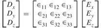
1.2 Free Space Propagation
In transmission media where the electric and current charges in Equations (1.11 to 1.14) are zero the solution of Maxwell's equations gives the following relationships:
1.18 ![]()
1.19 ![]()
Taking the curl of Equations (1.20) and (1.21), and using the identity in Equation (1.10), we obtain the free space wave equations:
1.22a ![]()
1.22b ![]()
1.3 Uniform Plane Wave Propagation
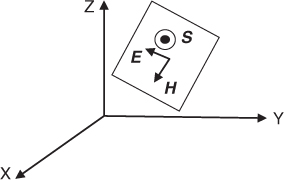
In uniform plane wave propagation the electric and magnetic field lines are perpendicular to each other and to the direction of propagation, as illustrated in Figure 1.1. This condition is satisfied if the electric and current charges are zero and the electric and magnetic fields are of a single dimension.
Figure 1.1 Electric field and magnetic field and direction of propagation of a plane wave.
For example, for a uniform plane wave propagating in the x direction, the electric and magnetic field lines can be along the y axis and the z axis respectively and the curl of Equation (1.20) gives:
A solution that satisfies Equation (1.23) is of the form:
where Eo is the amplitude of the wave, ![]() is the angular frequency in radians per second (rad/s) and
is the angular frequency in radians per second (rad/s) and ![]() 2π/λ is the wave number where f is the frequency in Hz and λ is the wavelength in m. Similarly, the magnetic field can be given by:
2π/λ is the wave number where f is the frequency in Hz and λ is the wavelength in m. Similarly, the magnetic field can be given by:
1.25 ![]()
where Ho is the amplitude of the magnetic field.
The ratio of the electric field to the magnetic field is an impedance η given by:
For a vacuum, Equation (1.26) becomes:
which is called the intrinsic impedance of free space.
If we select a point along the wave satisfying the condition:
1.28 ![]()
then the phase velocity of the wave, vp is given by:
In a vacuum the phase velocity is equal to the speed of light c = 3 × 10⁸ m/s.
The direction of propagation of a plane wave is determined from the Poynting vector S given by:
where the mean rate of flow of energy is the real part of S, that is:
The direction of propagation is therefore obtained by turning E into H and proceeding as with a right-handed screw, as shown in Figure 1.1, where the dot inside the circle indicates the tip of an arrow; that is the Poynting vector S is perpendicular to the plane of the electric and magnetic fields and gives the magnitude and direction of the energy flow rate as given in Equations (1.30a) and (1.30b).
1.4 Propagation of Electromagnetic Waves in Isotropic and Homogeneous Media
For propagation in matter we would need to solve Maxwell's Equations (1.11 to 1.14), which can include the conduction current and the charge. We start by studying plane wave propagation in different media, which are both isotropic and homogeneous, since these two properties apply to most gases, liquids and solids provided that the electric field is not too high. The combination of these two properties implies that the relative permittivity, relative permeability and conductivity are constant and that the permittivity is a scalar. This results in both D and E having the same direction.
Here we will consider two media of propagation: dielectric material and conductors.
For time-harmonic fields at ![]() the electric and magnetic fields can be written as:
the electric and magnetic fields can be written as:
Rewriting Equations (1.31a) and (1.31b) as a complex exponential and taking the derivative gives:
1.32a ![]()
1.32b ![]()
Equations (1.13) and (1.14) can now be expressed as:
Taking the curl of Equation (1.33) and using Equation (1.34) gives:
If the charge is zero, then the divergence of ![]() and Equation (1.35) reduces to:
and Equation (1.35) reduces to:
where
![]()
Solving for ![]() , we obtain:
, we obtain:

A possible solution for Equation (1.36) gives the following form for the electric field:
Similarly, a solution for H is:
Using Equation (1.39) in Equation (1.33) and taking the curl of E in Equation (1.38) gives:
1.40 ![]()
The ratio of the electric field to the magnetic field is again the intrinsic impedance η given by:
1.41 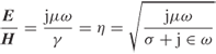
Using the definition of η in Equation (1.36) the electric field in Equation (1.38) can be expressed as:
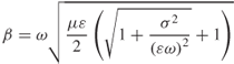
Equation (1.42) is the general equation for transverse propagation, which can be simplified for various special cases. In the equation α represents the attenuation factor, with units per metre (m−1) and indicates an exponential decay in the field strength with distance.
- Case 1: Free space propagation
- Case 2: Perfect dielectric
1.44 ![]()
- Case 3: Good dielectric
1.45 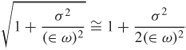
1.46a 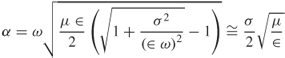
1.46b 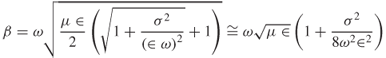
1.47 ![]()
- Case 4: Good conductor

1.48a ![]()
1.48b 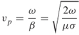
![]()
Considering the attenuation factor in Equation (1.42), we see that when the wave has travelled a distance ![]() , the wave would have been reduced to 1/e or 36.8 % of its original value. This distance is called the penetration depth or skin depth, designated as
, the wave would have been reduced to 1/e or 36.8 % of its original value. This distance is called the penetration depth or skin depth, designated as ![]() . For a good conductor this value is given by:
. For a good conductor this value is given by:
1.49 
- Case 5: Perfect conductor
Table 1.1 Propagation parameters in different isotropic and homogeneous media
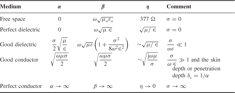
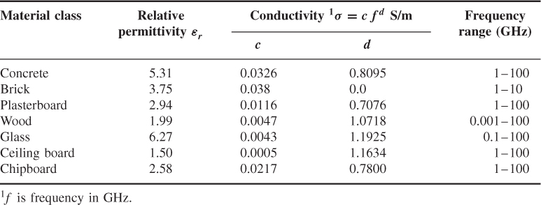
Table 1.2 Typical values of relative permittivity and conductivity for different building materials [3]
1.5 Wave Polarization
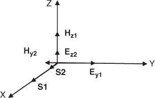
Polarization refers to the time varying behaviour of the electric field vector E at a certain point in space. Figure 1.2 illustrates transverse wave propagation where the wave has a single electric component along the y axis. In this case, the tip of the electric field E remains in the same direction but the instantaneous value of the electric field varies with time and space as given in Equation (1.24). Assume that there is another wave that is perpendicular and independent of the first wave and that also propagates in the x direction but has its magnetic and electric fields as shown in Figure 1.2.
Figure 1.2 Two planar waves propagating in the x direction but with their electric and magnetic fields being perpendicular.
Assume that the electric fields of the two waves are given by:
At x = 0, Equations (1.51a) and (1.51b) become:
1.52a ![]()
1.52b ![]()
The combination of these two waves gives rise to different polarizations depending on the relative amplitudes of the electric fields ![]() and
and ![]() and the phase difference δ between them.
and the phase difference δ between them.
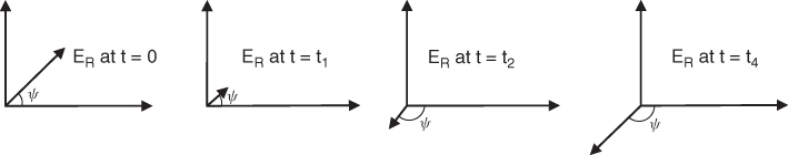
- Case 1: If
 , then the electric field components are in phase all the time and the resultant is given by:
1.53 ![]()
Figure 1.3 Variations of the electric field with time resulting from combining two independent transverse waves.
1.55 ![]()
- Case 2:

1.56b ![]()
Figure 1.4 Polarization ellipse.
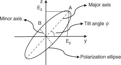
The axial ratio (AR) is given by the ratio of the major axis to the minor axis and is between 1 and ∞. Equation (1.58) can be viewed as the generalized case with special cases obtained for linear and circular polarization.
Linear polarization occurs in one of two cases:
A circularly polarized wave occurs when ![]() and Ey1 = Ez2. Substitution of these conditions in Equation (1.58) gives Equations (1.59a) and (1.59b), which represents a circle with AR = 1:
and Ey1 = Ez2. Substitution of these conditions in Equation (1.58) gives Equations (1.59a) and (1.59b), which represents a circle with AR = 1:
When ![]() we have a left circularly polarized wave and when
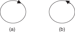
we have a left circularly polarized wave and when ![]() we have a right circularly polarized wave, as shown in Figure 1.5.
we have a right circularly polarized wave, as shown in Figure 1.5.
Figure 1.5 (a) Left- and (b) right-hand polarizations.
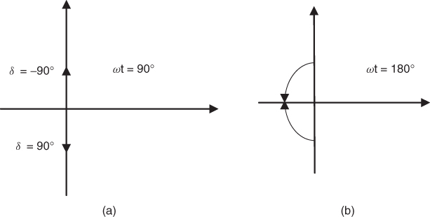
The two circular polarizations can be deduced by assuming ![]() ° and x = 0. Under these assumptions the electric field along the y axis is zero and the z component is equal to −E for
° and x = 0. Under these assumptions the electric field along the y axis is zero and the z component is equal to −E for ![]() and +E for
and +E for ![]() , as illustrated in Figure 1.6a. When
, as illustrated in Figure 1.6a. When ![]() t = 180° the electric field along the y axis becomes equal to zero and the electric field along the z axis becomes equal to −E for both
t = 180° the electric field along the y axis becomes equal to zero and the electric field along the z axis becomes equal to −E for both ![]() and, as shown in Figure 1.6b, the two components rotate in opposite directions, with that for
and, as shown in Figure 1.6b, the two components rotate in opposite directions, with that for ![]() rotating counter-clockwise and that for
rotating counter-clockwise and that for ![]() rotating clockwise.
rotating clockwise.
Figure 1.6 Illustration of the circular polarization for left-handed and right-handed polarizations.
Generally polarization is defined by a complex number:
1.60 ![]()
where
1.61 ![]()
That is the polarization is a function of the amplitude ratio of the two electric fields and the phase difference between them.
In summary linear polarization results if the phase difference between the two electric field components is 0° or 180°, circular polarization when the two electric field components are equal in amplitude but have a relative phase equal to ±90° or ±270° and the general case of elliptical polarization results for all other values of the relative amplitudes of the two waves and relative phases. Table 1.3 summarizes the resultant wave polarization.
Table 1.3 Summary of different cases of wave polarization
| Type of polarization | Relative magnitude of the electric field components Ey, Ez | Phase difference between Ey and Ez |
| Circular | Equal magnitude of Ey and Ez | ±π/2, ±3π/2 |
| Elliptical | Any magnitude of Ey and Ez | Any phase difference |
| Linear | Any magnitude of Ey and Ez | 0, π |
| Either Ez or Ey = 0 | Irrelevant |
1.6 Propagation Mechanisms
So far we have only considered propagation of an electromagnetic wave in a single medium. Generally, an electromagnetic wave travelling in real environments encounters a number of different media. Depending on the properties of these media a number of propagation mechanisms can occur at the interface, which include reflection, refraction, absorption, scattering and diffraction. In this section we study these different mechanisms and their effect on the resulting electromagnetic wave.
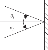
1.6.1 Reflection by an Isotropic Material
An electromagnetic wave incident on a medium whose dimensions are considerably larger than its wavelength undergoes reflection, which can be either specular or diffuse depending on the properties of the medium. Specular reflection is mirror-like, where the angle of incidence ![]() and the angle of reflection
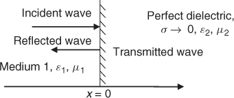
and the angle of reflection ![]() are equal, as shown in Figure 1.7. In this section reflection by a perfect conductor and a perfect dielectric will be considered both at normal incidence and at oblique incidence.
are equal, as shown in Figure 1.7. In this section reflection by a perfect conductor and a perfect dielectric will be considered both at normal incidence and at oblique incidence.
Figure 1.7 Specular reflection.
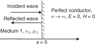
1.6.1.1 Case I: Normal Incidence
Figure 1.8 Reflection by a perfect conductor.
1.62a ![]()
1.62b ![]()
Figure 1.9 Reflection by a dielectric.
1.66 ![]()
1.67a ![]()
1.67b ![]()
1.68a ![]()
1.68b ![]()
1.69 ![]()
1.70a ![]()
1.70b ![]()
1.70c ![]()
1.70d ![]()
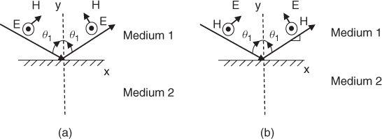
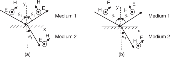
1.6.1.2 Case II: Reflection/Refraction at Oblique Incidence
When an electromagnetic wave is incident on a medium at oblique incidence, two waves result, where one is reflected in the same medium with an angle equal to the incident angle ϑ1 and a refracted or transmitted wave in the medium with an angle equal to ϑ2. Two cases arise depending on whether the electric field is parallel to the boundary surface (termed vertical polarization) or perpendicular to the plane of incidence of the wave (termed horizontal polarization), which occurs when the magnetic field is parallel to the boundary surface. In this case the electric field component can be resolved into two components, one parallel to the boundary surface and one perpendicular to it.
![]()
Figure 1.10 Reflection by a perfect conductor at oblique incidence: (a) perpendicular polarization and (b) parallel polarization.
1.72 ![]()
1.73 ![]()
1.74a ![]()
1.74b ![]()
Figure 1.11 Oblique incidence at a dielectric material.
1.75 ![]()
1.77 ![]()
1.79 ![]()
1.81 ![]()
Figure 1.12 Oblique incidence at a dielectric: (a) perpendicular incidence polarization and (b) parallel polarization.
1.83 ![]()
1.86 ![]()
1.87 ![]()
1.88 ![]()
1.90 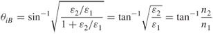
1.91 ![]()
1.6.2 Reflection/Refraction by an Anisotropic Material
In certain media the speed of propagation is not the same in all directions, such as in the case of calcite. This results in two indices of refraction known as double refracting or birefringent. The resulting waves are called ordinary and extraordinary waves where the ordinary wave has the same refractive index in all directions and the extraordinary wave has a variable refractive index as a function of direction. The effect is seen as a double image, which corresponds to the two waves shown in Figure 1.13.
Figure 1.13 The formation of two waves due to the anisotropic properties of calcite.

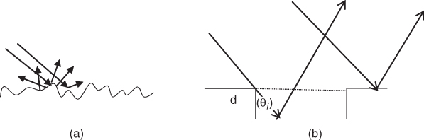
1.6.3 Diffuse Reflection/Scattering
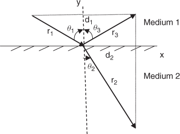
Diffuse reflection occurs when the incident wave impinges on a rough surface with dimensions comparable to the wavelength. In this case the wave is reflected in several directions, as shown in Figure 1.14a. A measure of roughness is given by the Rayleigh criterion, C. Referring to Figure 1.14b, the phase difference in path length between the rays reflected from different heights on the surface is equal to:
where ![]() is the angle of incidence of the wave on the rough surface. For d
is the angle of incidence of the wave on the rough surface. For d ![]() λ the phase difference between the two reflected rays is small and the surface is considered smooth, whereas if the phase difference is close to π, then the surface is considered rough. A rough surface is usually defined for values of phase difference greater than π/2 or, equivalently,
λ the phase difference between the two reflected rays is small and the surface is considered smooth, whereas if the phase difference is close to π, then the surface is considered rough. A rough surface is usually defined for values of phase difference greater than π/2 or, equivalently,
1.93 ![]()
Since surfaces generally have irregular shapes different from those of Figure 1.14b, it is usual to replace ![]() in Equation (1.92) in terms of the standard deviation of the ground undulations, σ, which results in the Rayleigh criterion, designated as C:
in Equation (1.92) in terms of the standard deviation of the ground undulations, σ, which results in the Rayleigh criterion, designated as C:
1.94 ![]()
For small angles of incidence C can be expressed as:
1.95 ![]()
The Rayleigh criterion is a measure of the roughness of the surface where, for C < 0.1, the surface is considered smooth, resulting in specular reflection, whereas for C > 10, there is highly diffuse reflection and the reflected wave is small enough to be neglected.
Figure 1.14 Diffuse reflection (a) from a random rough surface and (b) from a structured rough surface.
Scattering of light by the atmosphere occurs when light is incident on gas molecules of dimensions much smaller than the wavelength of incident light where the relative intensity is inversely proportional to ![]() . This means that higher frequencies are scattered more, which results in blue light being more scattered than red light, which results in the colour of the sky being blue. In the evening, light has to travel a longer distance, which gives rise to higher absorption of blue, resulting in the colour of the sky being red.
. This means that higher frequencies are scattered more, which results in blue light being more scattered than red light, which results in the colour of the sky being blue. In the evening, light has to travel a longer distance, which gives rise to higher absorption of blue, resulting in the colour of the sky being red.
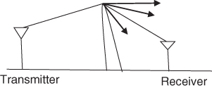
1.6.4 Diffraction
Another wave propagation mechanism is diffraction, which occurs when a wave encounters an obstacle. The effects of diffraction were first observed by Francesco Maria Grimaldi (1618–1663) who introduced the term diffraction from the Latin word diffringere, meaning breaking into pieces. Depending on the type of obstacle, two different phenomena are explained by the diffraction theory. One is the apparent bending of the wave such as over a hill top as in Figure 1.15. The second is the spreading out of waves past small openings such as in diffraction grating.
Figure 1.15 Diffraction over a hill top.
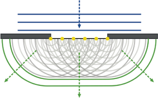
Diffraction is described by the Huygens–Fresnel principle, which states that every point on a wavefront acts as a point source for a secondary radial wave, as shown in Figure 1.16. The new waves interfere by adding constructively or destructively depending on the relative amplitude and phases of the new waves, where the resultant can vary in amplitude from zero to the sum of the waves, thereby giving rise to maxima and minima along the path of propagation. Interference from two slits was demonstrated in 1803 by Thomas Young.
Figure 1.16 Illustration of Huygen's principle where each point on the wavefront is a source as the wave interacts with the obstacle.
The form of a diffraction pattern in space can be estimated using the Fraunhofer diffraction equation for the far field or the Fresnel diffraction equation for the near field. Diffraction has great significance in wireless communication, where radio waves are diffracted by the edge of a building or over a hill to reach a user on the other side of a radio link that is optically not visible. For radio wave propagation, losses due to diffraction will be discussed in Chapter 2 in relation to transmission loss.
1.7 Propagation in the Earth's Atmosphere
To study the effects of the earth's atmosphere on the propagation of radio signals, it is useful to refer to Table 1.4 to identify the frequency ranges of the different bands of the spectrum.
Table 1.4 Frequency bands of the spectrum
| Frequency bands | Frequency range |
| Extremely low frequency (ELF) | <3 kHz |
| Very low frequency (VLF) | 3–30 kHz |
| Low frequency (LF) | 30–300 kHz |
| Medium frequency (MF) | 300 kHz to 3 MHz |
| High frequency (HF) | 3–30 MHz |
| Very high frequency (VHF) | 30–300 MHz |
| Ultra high frequency (UHF) | 300 MHz to 3 GHz |
| Super high frequency (SHF) | 3–30 GHz |
| Extra high frequency (EHF) | 30–300 GHz |
1.7.1 Properties of the Earth's Atmosphere
Figure 1.17 displays the temperature of the earth's atmosphere versus height and the electron density variations versus height along with classification of the layers in the earth's atmosphere. Two regions of interest for radio systems are the troposphere and the ionosphere, which enable communication beyond the horizon. These two layers are discussed here in terms of their properties and the propagation mechanisms that govern each layer.
Figure 1.17 Regions of the earth's atmosphere classified as a function of height, temperature and electron density.
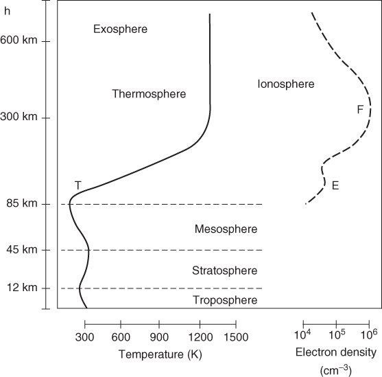
1.7.1.1 Troposphere
As seen from Figure 1.17, the troposphere is the lowest region of the earth's atmosphere and contains about 75 % of the atmosphere's mass and 99 % of its water vapour and aerosols. It starts from the earth's surface and extends to an average depth of about 17 km in the middle latitudes, being deeper in the tropical regions and shallower near the poles. The border between the troposphere and the stratosphere is called the tropopause and is characterized by temperature inversion where the temperature increases with height. Above 30 MHz, different properties of the refractive index of the troposphere give rise to different propagation effects.
The refractive index of the atmosphere n at the surface of the earth is approximately 1.0003, which is very close to unity. Because the changes in the value of n are very small, it is usual to use a scaled-up value of n, called the refractivity N, defined as N ![]() . N depends on the pressure p in millibars, the partial pressure of water vapour e in millibars and the absolute temperature T in Kelvin.
. N depends on the pressure p in millibars, the partial pressure of water vapour e in millibars and the absolute temperature T in Kelvin.
Two expressions commonly used for N are given in [1, Chapter 16] and [4, Chapter 7] as:
1.96a ![]()
and
1.96b ![]()
On average the radio refractivity N is equal to 301 at the surface and 260 at 1 km above the surface of the earth in temperate climates.
The temperature of the standard atmosphere decreases with altitude at the rate of 6.5 °C per kilometre. The standard moist atmosphere is specified as one with 10 millibars of water vapour pressure at sea level, decreasing with altitude by 1 millibar per thousand feet up to 10,000 ft [1, Chapter 16]. Variations in temperature and in moisture from the standard values result in variations in the dielectric constant and the resulting refractive index with height. Variations of N from the standard are represented by modified curves, called the M curves, which take the curvature of the earth into account.
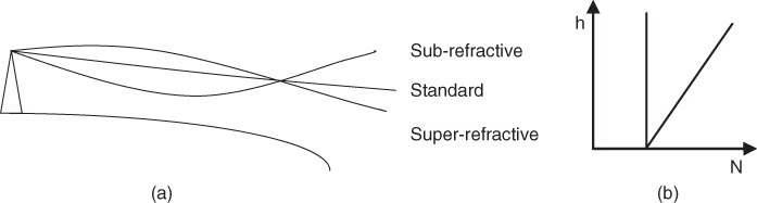
Depending on the variations of the modified refractive index with height, four propagation conditions are defined: standard propagation, superrefractive propagation, subrefractive propagation and ducting. Standard propagation occurs when the modified index of refraction increases linearly with height, whereas substandard (subrefractive) propagation arises when the M curve has a negative slope near the surface of the earth, which results in the rays curving upwards as illustrated in Figure 1.18. If the slope of the M curves increases at the surface of the earth, the upward curvature of the rays is less and superrefractive propagation results. If the M curve is vertical, there are no variations of the refractive index and the rays travel over a straight line; that is the rays have the same curvature as the earth.
Figure 1.18 (a) Refracted rays for different refractivity slopes [4, Chapter 7] and (b) linear increase and vertical or zero slope variations of refractivity with height.
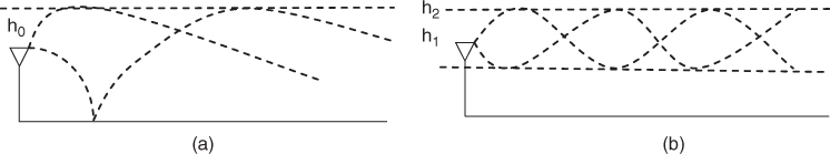
When the modified index decreases with height, the rays will be curved downwards and a condition known as trapping or duct propagation occurs. Ducts can be surface ducts or elevated ducts, as illustrated in Figure 1.19, depending on the relationship of the lower edge of the duct with respect to the surface of the earth. If the receiving antenna is elevated to within the duct, the received signal strength can be very large, whereas if the antenna is below or above the duct the signal strength will be very low. Elevated ducts are at a height of about 1000–5000 ft and have a thickness from a few feet to a thousand feet. Depending on the thickness of the duct, a critical frequency exists below which duct propagation will not occur. Ducting is a phenomenon that is usually associated with the ultra high frequency (UHF) band rather than the high frequency (HF) band due to the required thickness of the duct.
Figure 1.19 (a) Surface duct and (b) elevated duct.
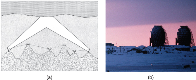
Another effect that gives rise to extended ranges of propagation in the troposphere is forward scattering, shown in Figure 1.20a, as contrasted to line of sight propagation. This arises from relatively sharp variations in the effective dielectric constant. Frequencies scattered from the troposphere are in the range of 100–10,000 MHz with bandwidths sufficient to enable transmission of television signals. An example of a radio communication system that relied on troposcatter is the White Alice Communication System (WACS) shown in Figure 1.20b, which used billboard antennas. The WACS system was installed in Alaska in the 1950s for communication as a distant early warning system for the US air force. Most of the system was deactivated towards the end of the 1970s.
Figure 1.20 (a) Troposcatter propagation and (b) billboard antennas used in the WACS system.
1.7.1.2 Ionosphere
Referring to Figure 1.17, the ionosphere is seen to incorporate the mesosphere and parts of the thermosphere. The mesosphere is characterized by decreasing temperature with height and extends from 50 to 85 km whereas the thermosphere includes the region above 85 km where the temperature increases steadily with height.
The ionosphere has a significant influence on radio wave propagation. Prior to satellite communications, the ionosphere was the only medium for long range radio links. The first experiments involving communication via the ionosphere were reported by Nikola Tesla in 1899 who conducted wireless telegraphy experiments transmitting signals from Pikes Peak to Paris. On 12 December 1901, Guglielmo Marconi received the first trans-Atlantic radio signal in St John Newfoundland with a transmitting station in Cornwall using a spark gap transmitter to produce a High Frequency signal of about 500 kHz. Although this experiment is contested, Marconi did achieve transatlantic wireless communications one year later in Glace Bay. In 1902, Oliver Heaviside and Arthur Edwin Kennely proposed independently the presence of an ionized region and discovered some of the ionospere's radio electrical properties. In 1926, Robert Watson-Watt introduced the term ionosphere and in 1927 Sir Edward Appleton confirmed the presence of the ionosphere, while its height was first measured by Lloyd Berkner.
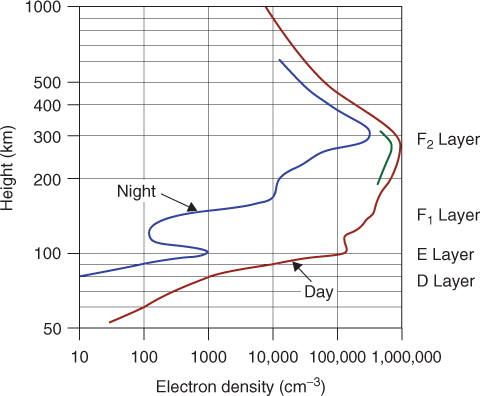
The ionosphere is formed by ionization of the atmosphere's gases, by the incoming ultraviolet and X-ray radiation from the sun. Due to the mixture of gases, which consist of oxygen, nitrogen, helium and hydrogen, and the nonmonochromatic radiation, as shown in Figure 1.21 [5], different ledges of ionization are formed and these are called the E layer at about 100 km, also known as the Kennely–Heaviside layer, and the F layer, which in the summer splits in the daytime into two ledges called F1 and F2. The layer below the E layer is called the D layer and has a very low density of electrons and can only reflect very low frequency (VLF). At HF the D layer is the main source of absorption of radio waves. In the summer, May–June, an intensely ionized strata called sporadic E, designated Es, caused by wind shears in the E layer develops at about 110 km altitude. A sporadic E layer can support propagation to high frequencies that extend up to 225 MHz.
Figure 1.21 Electron density profile versus height [7].
Source: Davies, K., (1990), Ionospheric Radio, The Institute of Electrical Engineers London. Reproduced with permission of IEE.
Since the electron density is dependent on the radiation intensity, the ionization varies diurnally, seasonally and with the sun activity, which follows a sun spot cycle of 11.4 years. For example, the D and E layers appear at sunrise and disappear at sunset and all vestige of the F1 layer disappears at night. There is also a tendency for the F2 peak to fall at dawn and to rise during the afternoon or evening. The ionization of the layers increases with the sunspot number R, which varies from 0 to 200 with the peak occurring at greater heights. In the northern hemisphere the F2 layer suffers from the winter anomaly where the electron intensity in the summer is lower than in the winter. This anomaly is more pronounced at high sunspot numbers. Propagation in the ionosphere is also affected by the presence of the earth's magnetic field and hence it is often referred to as a magneto-ionic medium.
1.7.2 Radio Waves in the Ionosphere
The ionosphere can be considered as a low conductivity dielectric with a refractive index less than unity, which decreases as the electron density increases or as the frequency decreases.
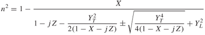
At extremely low frequency (ELF) and VLF the D region and the earth's surface form a waveguide with a single mode (with a vertical electric field). At medium frequency (MF) and HF propagation may be represented by refracted rays. Ionospheric propagation is also governed by the presence of the earth's magnetic field. By assuming a steady state solution for a simple harmonic progressive plane wave with a given polarization, Appleton derived a formula (known as the Appleton–Hartree equation) for the refractive index n of the ionosphere based on the following properties:
where
![]()
Here ω is the wave frequency, e and m are the charge and mass of an electron respectively, v is the frequency of collision between electrons and molecules, ![]() is the permittivity of free space, N is the electron density and
is the permittivity of free space, N is the electron density and ![]() are the earth's magnetic induction components in the direction transverse and parallel to the direction of wave propagation respectively. Derivation of the formula and a detailed treatment of ionospheric propagation can be found in [6, 7].
are the earth's magnetic induction components in the direction transverse and parallel to the direction of wave propagation respectively. Derivation of the formula and a detailed treatment of ionospheric propagation can be found in [6, 7].
Neglecting the earth's magnetic field and collisions, the refractive index n can be written as:
Using Snell's law for refraction where the refractive index at entry is 1 for free space and at reflection the angle is 90° gives:
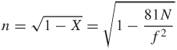
For vertical incidence ϑ1 is equal to zero and Equation (1.99) gives the plasma frequency fN or the vertically reflected frequency fv:
1.100 ![]()
For maximum ionization, the reflected frequency is the highest and is called the critical frequency. For all other angles of oblique incidence the reflected frequency fob is given by:
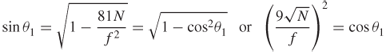
Equation (1.101) indicates that the reflected frequency depends on both the electron density, which varies as a function of height, and the angle of incidence. Due to these variations, it is possible to have two rays that satisfy Equation (1.101); these are called the high angle ray, known as the Pederson ray, reflected from a high layer and the low angle ray reflected from a low layer. At the maximum frequency and for certain path geometry, these two rays merge together and the signal strength is enhanced. The presence of the different layers such as the E and the F layers also presents possible paths that link the transmitter to the receiver. These can be either single reflections such as 1F, 1E or multiple reflections such as 1F2 and 2E2. Each path can also have its low and high angle rays and for long paths, higher order paths (modes) are received with comparable signal strength and a longer time delay, as illustrated in Figure 1.22. The maximum frequency of these modes is not much less than the first order mode, which arises from the secant law. The different modes of propagation for a particular path are measured using ionosondes, which can be operated vertically or over oblique paths to identify the propagation paths.
Figure 1.22 Possible modes of propagation in the ionosphere: (a) 1F, (b) 2E, (c) 1F2E, (d) N mode and (e) M mode.
Considering now Equation (1.97) including the effect of the earth's magnetic field but excluding the effect of collisions, the refractive index n becomes:
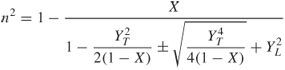
At the level of reflection for vertical incidence n = 0. Solving Equation (1.102) for X gives:
and
Substituting for YT and YL in Equation (1.103b) we get:
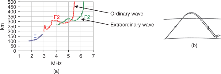
In Equation (1.104) fH is known as the gyro-frequency and is seen to depend on the strength of the earth's magnetic induction. Equations (1.103a) and (1.103b) shows that there are two waves, one wave called the ordinary wave or o-wave, which is independent of the magnetic field Y and another wave called the extraordinary wave or x-wave, which is a function of the magnitude of the earth's magnetic field and not its direction. The two waves are referred to as the magneto-ionic waves. Since in the ionosphere X is a positive number greater than zero, then for frequencies greater than the gyro-frequency the level of reflection is given by X = 1 − Y and for frequencies less than the gyro-frequency the level of reflection is given by X = 1 + Y. Hence, the effect of the earth's magnetic field is to add another component where the ordinary wave nearly follows the path of transmission, as in the absence of the earth's magnetic field. The two waves are illustrated in the ionogram of Figure 1.23, which is a plot of the height of reflection of the rays versus frequency.
Figure 1.23 Splitting into the two magneto-ionic waves: (a) ionogram displaying the E and F2 modes of propagation including the ordinary and extraordinary waves and (b) sketch of the two waves.
Substituting in Equations (1.103a) and (1.103b) for X and Y at the critical frequency of the layer we get:
1.105 ![]()
where fo and fx are the critical frequencies for the ordinary and extraordinary waves respectively.
If the critical frequency of the extraordinary wave is much greater than the gyro-frequency, as in the case of the ionosphere (fH ≅ 1.4 MHz), this gives the following relationship:
1.106 ![]()
This implies that the extraordinary wave persists to a frequency higher by an amount on the order of half the gyro-frequency; that is the trace of the extraordinary wave can be found from the trace of the ordinary wave by slipping it to the right by half the gyro-frequency, as seen in Figure 1.23.
For oblique propagation, the difference between the two waves depends on the geometry of the path and the geographic location. For east–west propagation, the separation in the USA was found to fall from 0.8 to 0.2 MHz in a range of variation of 0–3000 km [8], whereas for north–south paths the frequency separation between the two waves is always equal to the gyro-frequency regardless of distance.
The presence of the earth's magnetic field also affects the polarization of the wave. In the absence of the magnetic field the electrons oscillate in the direction of the incident electric field and reradiate in the same direction with the same polarization. In the presence of the electric field, the electrons will be subject to both the electric and magnetic fields and they will reradiate with a different polarization, which changes as the wave progresses through the ionosphere. From magneto-ionic theory, the wave's polarization R, neglecting collisions, is given by:
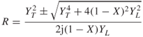
where the negative sign refers to the ordinary wave and the positive sign for the extraordinary wave [5]. Equation (1.107) gives the ratio of the complex amplitude of the orthogonal components of the electric field vector along the two axes perpendicular to the direction of propagation. In general the tip of the electric field vector describes an ellipse.
Two special cases arise when the ray propagation is along the earth's magnetic field (called longitudinal propagation), for which ![]() , and when it is transverse to it (called transverse propagation), for which
, and when it is transverse to it (called transverse propagation), for which ![]() . In the first case,
. In the first case, ![]() and Rx = −j and the two waves are circularly polarized with an opposite sense of rotation, whereas in the second case,
and Rx = −j and the two waves are circularly polarized with an opposite sense of rotation, whereas in the second case, ![]() and
and ![]() . This means that the polarization of the electric vector of the ordinary wave is linear and parallel to the external magnetic field. The electric vector of the extraordinary wave is also linearly polarized and lies in the plane perpendicular to the earth's magnetic field. In these two cases the polarization is independent of X, the operating frequency and the electron density. This is not the case for other incident angles between the ray and the earth's magnetic field.
. This means that the polarization of the electric vector of the ordinary wave is linear and parallel to the external magnetic field. The electric vector of the extraordinary wave is also linearly polarized and lies in the plane perpendicular to the earth's magnetic field. In these two cases the polarization is independent of X, the operating frequency and the electron density. This is not the case for other incident angles between the ray and the earth's magnetic field.
Since the wave polarization generally varies with X as seen from Equation (1.107), the polarization ellipses vary from one region of the ionosphere to another. At the level of reflection of the ordinary wave X = 1, the polarization ellipse R has a value equal to 0. At this point the electric vector of the ordinary wave is linearly polarized along the magnetic field whereas the extraordinary wave is linearly polarized but is oriented across the magnetic field.
In general, however, in the absence of collisions the electric field vectors of the ordinary and extraordinary waves are always elliptically polarized (except for longitudinal and transverse propagation), where for the ordinary wave the major axis is along the direction of the magnetic field at the point of exit from the ionosphere whereas it is transverse to it for the extraordinary wave. For a linearly polarized wave incident on the ionosphere, it splits into two circularly polarized waves.
1.8 Frequency Dispersion of Radio Waves
The phase velocity vp of a wave consisting of a single frequency was defined in Equations (1.29) and (1.43) as:
![]()
In vacuum, the phase velocity ![]() , where
, where ![]() is the wavelength in free space. In certain media such as the ionosphere, the phase velocity is a function of frequency. This can be related to Equation (1.98), which gives the refractive index n and the relationship between the refractive index and the phase velocity:
is the wavelength in free space. In certain media such as the ionosphere, the phase velocity is a function of frequency. This can be related to Equation (1.98), which gives the refractive index n and the relationship between the refractive index and the phase velocity:
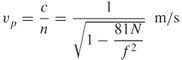
1.108b ![]()
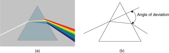
In such a medium where different frequencies travel over different path lengths with different velocities, the medium is called dispersive. The term was first used for the dispersion of colours by a prism and results in the resolution of the constituent colours in white light, as seen in Figure 1.24.
Figure 1.24 Dispersion of white light in a prism: (a) spectrum of light and (b) schematic of dispersion.
In radio communications a band of frequencies is transmitted to carry information where a carrier is modulated by a baseband signal. If the signal is transmitted in a dispersive medium, such as the ionosphere, where different frequencies travel over different path lengths, we must determine the velocity of the modulation or the velocity of energy. This leads to the definition of modulation velocity, also called group velocity.
1.8.1 Phase Velocity versus Group Velocity
To define group velocity let us assume two waves E1 and E2 travelling in the x direction:
1.109a ![]()
1.109b ![]()
The resultant E can be written as:
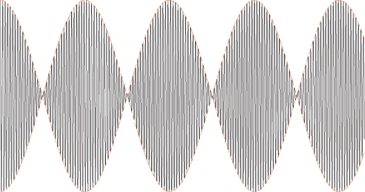
Equation (1.110) represents the superposition of two waves that produces a beat signal as shown in Figure 1.25 with an envelope given by:
Equation (1.111) gives a group velocity ![]() :
:
For example, for a wave with ![]() and
and ![]() , the phase velocities of the two waves are 1 and 0.9683 m/s respectively. From Equation (1.112) the velocity of the envelope is 0.333 m/s whereas the phase velocity of the internal oscillations is 0.9837 m/s. When the velocities of the two waves in the medium are the same, the peak of the beat signal will travel with the wave and the medium is called nondispersive.
, the phase velocities of the two waves are 1 and 0.9683 m/s respectively. From Equation (1.112) the velocity of the envelope is 0.333 m/s whereas the phase velocity of the internal oscillations is 0.9837 m/s. When the velocities of the two waves in the medium are the same, the peak of the beat signal will travel with the wave and the medium is called nondispersive.
Figure 1.25 Resultant of two waves with different frequencies travelling with different velocities.
There are two types of dispersive media: normally dispersive media and anomalously dispersive media, where:
1.113a ![]()
1.113b ![]()
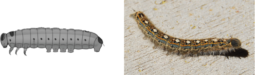
The effect of a normally dispersive medium is similar to that of a caterpillar where the humps move at the phase velocity but the whole caterpillar moves at the group velocity (Figure 1.26).
Figure 1.26 Illustration of phase and group velocity in terms of caterpillar movement.
If the low frequency component travels at a higher velocity than the high frequency component, then the envelope appears to be moving ahead of the carrier.
The concept of the group velocity is not applicable under conditions of severe distortion as can occur in a highly dispersive medium. It applies when the modulation envelope retains its shape, which occurs when the group velocity is a constant within the group, that is:
1.115 ![]()
Taking the derivative of:
![]()
This equation can be rewritten to give the following alternative expressions for the group velocity:
1.116 ![]()
1.8.1.1 Group Refractive Index
By analogy to the phase refractive index n, a group refractive index ![]() can be defined as:
can be defined as:
Using Equation (1.108) for ionospheric propagation, the group refractive index reduces to:
1.118 ![]()
1.8.2 Group Path versus Phase Path
Since the phase and group velocities are not identical, the transit time of the surface of constant phase ![]() and the wave packet
and the wave packet ![]() are different. This in turn leads to the definition of phase path and group path. To find the group path, we consider an element of length
are different. This in turn leads to the definition of phase path and group path. To find the group path, we consider an element of length ![]() travelled by the wave packet in a medium of refractive index
travelled by the wave packet in a medium of refractive index ![]() . This gives:
. This gives:
1.119 ![]()
The total time of flight ![]() is given by:
is given by:
By analogy, the phase time ![]() is given by:
is given by:
Using Equation (1.117), the group path equation can be written as:
1.122 ![]()
Therefore,
1.123 ![]()
where ![]() is the phase retardation along the path.
is the phase retardation along the path.
The phase path P and the group path P′ can be found by multiplying Equations (1.120) and (1.121) by c, which gives the following relationship:
1.124 ![]()
Ionogram measurements as in Figure 1.23 display the group path versus frequency where the phase path can be obtained by expanding the phase ![]() in a Taylor series around a centre frequency:
in a Taylor series around a centre frequency:
1.126 ![]()
Truncating after the second term and substituting for the group time, the phase versus frequency function can be related as in Equation (1.127) to the derivative of the group time delay:
Equation (1.127) can be used to estimate the distortion suffered by a signal due to the frequency dispersion effects of the medium, as discussed in Section 3.3.1.
1.8.3 Phase Path Stability: Doppler Shift/Dispersion
Phase path variations can be attributed to either the movement of the medium, such as the movement of the reflecting layers in the ionosphere while both the transmitter and receiver are stationary, or the movement of either the transmitter or the receiver or a combined effect. The effect on a CW signal is observed as variations in the transmitted frequency that can be related to the rate of change of the phase path length. This can be illustrated by considering a CW signal with frequency ![]() and relative varying time delay
and relative varying time delay ![]() with respect to the transmitted signal:
with respect to the transmitted signal:
Taking the derivative of the phase, the instantaneous frequency ![]() can be found as:
can be found as:
1.129 ![]()
where ![]() is called the Doppler frequency after the Austrian physicist Christian Doppler who proposed it in 1842. Since the time delay and the phase path are related, the Doppler frequency can be rewritten as:
is called the Doppler frequency after the Austrian physicist Christian Doppler who proposed it in 1842. Since the time delay and the phase path are related, the Doppler frequency can be rewritten as:
1.130 ![]()
If the phase path variations are constant, then the Doppler frequency will be a constant. However, if the phase path variations are time-variant, then a Doppler spread will appear around the carrier.
References
1. Jordan, E.C. and Balmain, K.G. (1968) Electromagnetic Waves and Radiating Systems, Prentice Hall, New York.
2. Kraus, J.D. and Fleisch, D.A. (1999) Electromagnetics with Applications, McGraw-Hill Book Co., New York.
3. ITU, Recommendation ITU-R P.1238-7, Propagation data and prediction methods for the planning of indoor radiocommunication systems and radio local area networks in the frequency range 900 MHz to 100 GHz.
4. Barcley, L. (2003) Propagation of Radio Waves, The Institution of Electrical Engineers, London.
5. Kelso, J.H. (1964) Radio Ray Propagation in the Ionosphere, McGraw-Hill Book Co., New York.
6. Budden, K.G. (1961) Radio Waves in the Ionosphere, Cambridge University Press, Cambridge, MA.
7. Davies, K. (1990) Ionospheric Radio, The Institution of Electrical Engineers, London.
8. Davies, K. (1965) Ionospheric Radio Propagation Monograph, NBS Monograph, Vol. 80, US Department of Commerce.