Chapter 2
Radio Wave Transmission
Radio systems form part of our daily routine and their applications are diverse. Examples include (i) long range and short range radio communications and on-body radio networks, (ii) radio imaging, (iii) radio remote sensing and (iv) radio frequency identification. The successful implementation of such systems requires knowledge of how radio waves are transmitted in various media and the available power to the receiver. Transmission loss, also known as path loss or attenuation, refers to the gradual loss of power density of a signal in a medium. This phenomenon applies to a number of areas other than radio transmission, such as the attenuation of sound and light in sea water, and losses over an optical link or electric power transmission line. Attenuation in a radio or an optical fibre link limits the rate of digital data transmission and hence has to be taken into account when designing a communication system. While in optical fibre the main source of attenuation is due to scattering, a number of factors contribute to transmission loss of radio waves such as atmospheric effects, terrain and propagation through buildings. Estimation of transmission loss is important in ensuring an acceptable quality of service by locating transmitters at appropriate locations and with appropriate power levels to provide coverage over the desired geographic area.
This chapter discusses transmission loss starting with the basic form of propagation in free space to transmission loss due to scattering and absorption in natural media such as the troposphere and the ionosphere. Typical measured transmission loss into buildings and vehicles are then given. This is followed by studying various propagation models, which include diffraction loss models, and the effect of ground reflection in the presence of a direct path between the transmitter and receiver. The resultant two-ray model is derived and its properties are discussed. The two-ray model is applied to both terrestrial environments and to the magneto-ionic waves in the ionosphere. Multipath propagation is then discussed for both long range communication via the ionosphere and for indoor and terrestrial communication in built-up areas.
2.1 Free Space Transmission
2.1.1 Path Loss
The free space path loss equation is derived under the far field assumption where the propagation distance d that separates the transmitter and receiver is much larger than D, which is the largest physical linear dimension of the antenna. In addition:
Under these assumptions the radiated energy is spread over the surface of a sphere, as shown in Figure 2.1, where the power density S in units of watts per m2 (W/m2) at distance d is equal to:
where 4πd2 is the surface area of the sphere of radius d and PT is the transmitted power (watts).
Figure 2.1 Illustration of the decrease of power density with distance.
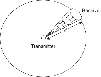
Figure 2.1 shows that the density of flux lines decreases as the distance increases away from the source. The available power PR in watts (w) at the receive antenna with effective area A, is given by:
where GR is the gain of the receive antenna given by:
The effective area of the antenna A is also known as the aperture of the antenna and is the area of a circle constructed broadside to the incoming radiation where all radiation passing through the circle is delivered to a matched load. Equation (2.2) can be rewritten to express path loss, which is the ratio of the transmitted power to the received power. For an isotropic receive antenna with unity gain this gives:
where f is the frequency (Hz) and c is the speed of light (m/s). Expressing Equation (2.4) in decibels (dB), the free space path loss Lf is given as:
It is often more convenient to work with the frequency expressed in MHz and distance in km. In this case, Equation (2.4) becomes ![]() and Equation (2.5a) becomes:
and Equation (2.5a) becomes:
2.5b ![]()
When the transmit antenna and the receive antenna have gains greater than unity, and are equal to GT and GR respectively, the effective (or equivalent) isotropic radiated power (EIRP) of the transmitter is equal to the product GT PT and Equation (2.4) becomes:
The received signal power in decibels is then expressed as:
Equations (2.4) to (2.7) are the ‘free space’ equations, also known as Friis equations. Since the antenna does not create energy, an increase in the antenna gain means that the power is radiated preferentially in a particular direction, leading to an increase in received power. Thus, Equations (2.6) and (2.7) show that path loss decreases as the directivity of antennas increases. High gain antennas can be used to compensate for the transmission loss and such antennas are relatively easy to design at frequencies in and above the VHF band.
Equation (2.5a) shows that: (i) free space transmission loss obeys a square law with range d, so that the received power falls by 6 dB when the range is doubled or reduced by 20 dB when the range is multiplied by 10, that is 6 dB/octave or 20 dB/decade, and (ii) path loss also increases with the square of the transmission frequency, in a similar way to distance. However, caution should be used here in interpreting the frequency dependence as it was introduced into the equation when the aperture of the antenna was expressed in terms of gain and wavelength and not due to free space propagation. In addition, the loss of received power is due to the limited aperture of the receive antenna, which is not capable of collecting all the transmitted power that is dispersed in space. Note that the Friis equation cannot be used for d = 0, and usually a reference distance do ≥ df is used for the close-in power. For practical systems in the 1–2 GHz range do is typically 1 m in indoor environments and 100 m or 1 km in outdoor environments.
The free space equation can also be rewritten in terms of the power received at two different distances as:
Setting d1 = do, Equation (2.8) can be used to find the power at distances greater than do.
2.1.2 Relating Power to the Electric Field
While cellular telephone operators mostly calculate the received power, in the planning of the coverage area of broadcast transmitters, it is recommended to use the root mean square (RMS) of the electric field strength E at the location of the receiver. Relating the power density S (W/m2) to E (V/m) and equating it to Equation (2.1) with a transmit antenna gain GT gives the following relationship:
2.9a ![]()
or
2.9b ![]()
where Zo = η = 120π Ω = 377 Ω is the characteristic wave impedance of free space.
Using Equation (2.2) and substituting Equation (2.3) for the antenna aperture the received power that can be delivered to the terminals of a matched receiver is given by:
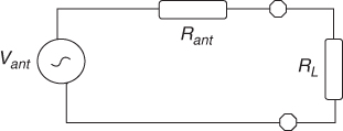
For an antenna with impedance Rant connected to a load impedance RL, as illustrated in Figure 2.2, the power delivered to a matched load can be related to the RMS voltage across the antenna terminals as:
2.11 ![]()
Equation (2.10) can also be written in logarithmic form with appropriate conversion parameters for dBW or dBm.
Figure 2.2 Antenna equivalent circuit with a matched load.
2.2 Transmission Loss of Radio Waves in the Earth's Atmosphere
The transmission loss considered so far relates only to the geometric spreading of energy and the limited aperture of the receive antenna where the medium of transmission is lossless. In this section we consider attenuation losses due to nonideal media of transmission, where attenuation is measured in decibel units per unit length of travel in the medium such as dB/cm or dB/km and these are related to the attenuation coefficient of the medium.
2.2.1 Attenuation due to Gases in the Lower Atmosphere and Rain: Troposphere
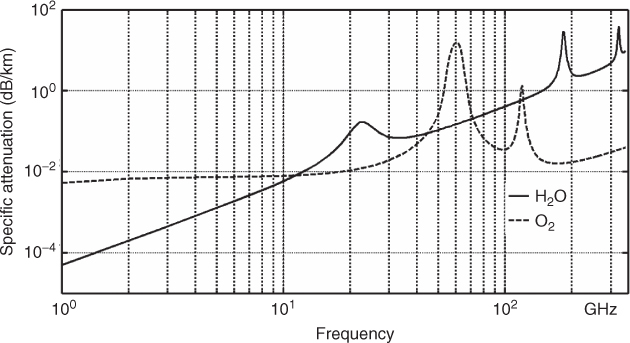
In radio transmission on the air attenuation occurs due to two mechanisms: absorption by gases and scattering by snow, hail, fog and rain. These effects have been quantified from measurements documented in various recommendations of the International Telecommunication Union (ITU). For most practical applications at frequencies below 30 GHz, rain is the main source of attenuation. For frequencies above 100 GHz, attenuation in fog becomes significant with attenuation coefficients between 0.4 and 4 dB/km for medium fog to thick fog. Molecular absorption by water vapour H2O and oxygen O2 are also important for high frequencies where resonances resulting in absorption peaks occur at certain frequencies. For example, the oxygen resonance at 60 GHz and 140 GHz and the peak of absorption by water vapour at 22 GHz are shown in Figure 2.3 [1]. However, at these frequencies attenuation due to rain is much more significant. Links operating at these resonance frequencies thus tend to be limited in range. For example, for a 10 km link, the rain attenuation for 0.0001 % of the time is around 40 dB, which makes the 1.7 dB water vapour attenuation negligible [2].
Figure 2.3 Plot of absorption versus frequency due to atmospheric gases: oxygen and water vapour.
Rain attenuation is related to the drop size distribution and is frequency and polarization dependent with horizontally polarized waves being more attenuated than vertically polarized waves [3, 4]. Generally for European climates it is not significant for frequencies below 11 GHz, whereas in monsoon climates and regions of severe storm, the critical frequency can be as low as 5 GHz, in which case rain attenuation needs to be considered.
The ITU-R procedure for the computation of rain attenuation, AP, where the subscript P stands for the percentage of time, is based on an empirical model given by:
where A0.01 represents the attenuation at 0.01 % of the time and is given by:
where d is the path length of the link and:
R0.01 in units of mm/h is the rain rate at 0.01 % of the time obtained from measurements with 1 minute integration time and kp and αp are regression coefficients where the subscript p refers to polarization.
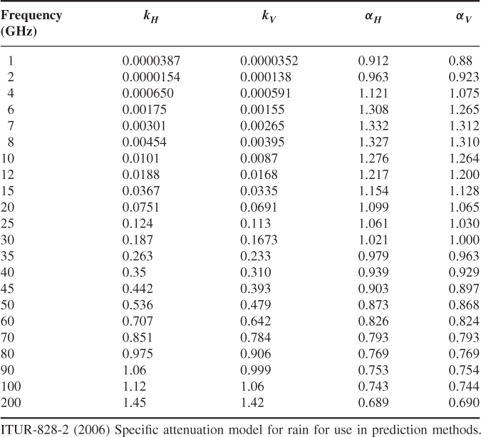
Values of rain rates are tabulated in ITU-R P 837 and ITU-R 530 presents a model for rain attenuation based on rain rates at 0.01 % of the time. Monthly mean rain rate values in mm/h are presented in Table 2.1 for the London area. These were gathered by the Global Historical Climatology Network (http://www.worldclimate.com/), which collects data from about 7500 precipitation stations. Table 2.2 gives ITU-R P 838 values for the coefficients in Equation (2.13c) versus frequency for mid latitudes for both horizontal kH, αH and vertical kV, αV polarizations [5]. These values in conjunction with Equations (2.12) and (2.13a), (2.13b) and (2.13c) can be used to compute the attenuation for different percentages of time. For example, for 1, 0.1, 0.01 and 0.001 %, Equation (2.12) has the values of 0.12, 0.39, 1 and 2.14 respectively. The empirical model of Equation (2.12) does not take into account the variations of rainfall at different points along the link experienced in practice, in particular over long links and those in mountainous terrain.
Table 2.1 Monthly mean rain rates in the London area over 358 months (1961–1990)
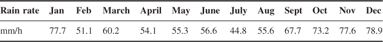
Table 2.2 Values for regression coefficients for vertical and horizontal polarizations as a function of frequency [5]
For example, to estimate the rain attenuation over a path of 20 km at 10 GHz, of a vertically polarized wave, in January and July in the London area using Equation (2.13b) gives: γ = 2.133 dB/km, do = 10.9118 km and r = 0.353, which gives a path attenuation of 15.06 dB for January and γ = 1.0635 dB/km, do = 17.874 km and r = 0.4719, which gives a path attenuation of 10.04 dB for July, which is ∼5 dB difference.
An alternative to the ITU-R procedure outlined above is a UK model described in [2, pp. 59–60], which takes the variations of the rain rate along the path into account. However, the difference between the two methods as shown in [2] is within 2 dB and hence the ITU-R model is a good guide to use, particularly for regions where rain rate data are not available.
2.2.2 Attenuation of Radio Waves in an Ionized Medium: Ionosphere
When an electromagnetic wave encounters free electrons, the electric field of the wave transfers energy to the electrons, which vibrate in the direction of the electric field. These vibrations lead to collisions with other electrons, molecules or ions, which give rise to dissipation of energy. The amount of dissipated energy depends on the density of molecules and the wavelength of the electromagnetic wave. Long wavelengths cause larger displacements of electrons, thus increasing the possibility of collisions and attenuation. As the frequency of the wave is increased, the displacement of electrons decreases, with the overall effect of reduced attenuation. In addition, as the density of molecules increases, the probability of collision increases, giving rise to a higher level of attenuation.
The effect of collisions on the refractive index of the ionosphere can be deduced from Equation (1.97) by neglecting the effect of the earth's magnetic field. This gives the following expression for the refractive index n:

where ![]() is the plasma frequency and ω is the angular frequency of the wave in rad/s. Equation (2.14) indicates that the refractive index n is complex, where the imaginary part, which is responsible for the attenuation of electromagnetic waves, arises due to collisions.
is the plasma frequency and ω is the angular frequency of the wave in rad/s. Equation (2.14) indicates that the refractive index n is complex, where the imaginary part, which is responsible for the attenuation of electromagnetic waves, arises due to collisions.
The effect of collisions can be illustrated by considering three cases, which depend on the relationship between the frequency of the wave ω in relation to the frequency of collision ν. When ![]() as in the F layer (ν is on the order of 5 kHz) the refractive index can be considered to be real and the ionosphere acts as a totally reflecting dielectric for high frequencies. When ω > ν, as in the E layer, waves suffer small attenuation whereas when ω < ν, as in the D layer (ν is on the order of 75–200 kHz), the ionosphere acts as a conductor.
as in the F layer (ν is on the order of 5 kHz) the refractive index can be considered to be real and the ionosphere acts as a totally reflecting dielectric for high frequencies. When ω > ν, as in the E layer, waves suffer small attenuation whereas when ω < ν, as in the D layer (ν is on the order of 75–200 kHz), the ionosphere acts as a conductor.
The attenuation of radio waves can be related to the concentration of electrons and molecules, which vary between the layers, as shown in Figure 1.17. For example, the D layer and the lower parts of the E layer have a high density of molecules, which increases the chances of collisions. Hence, these layers are the main source of attenuation of medium wave radio broadcasts, so that during the daytime they only propagate via a ground wave. At night when the D layer disappears, radio broadcasts can be heard at very long distances. Attenuation of radio waves in the D layer gives rise to a critical frequency called the lowest usable frequency (LUF), which is the lowest frequency at which communication between two points can be achieved.
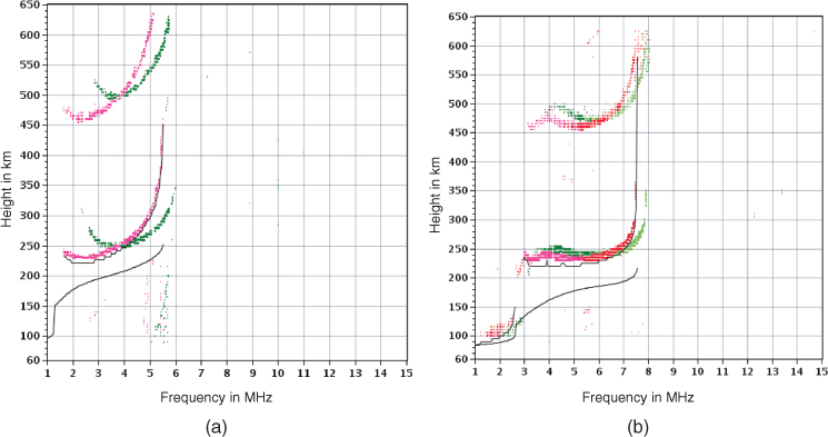
As the frequency is increased, attenuation decreases by the inverse square law. However, as the frequency increases its reflection height also increases as it requires a higher electron density. This gives rise to another critical frequency called the maximum usable frequency (MUF), beyond which electromagnetic waves go through the ionosphere without being reflected. Since the electron density varies continuously as electrons are generated and recombined with ions, for reliable communication it is usually recommended to operate at a frequency lower than the MUF. This frequency is called the optimum working frequency and is usually between 0.8 and 0.85 of the MUF. Figure 2.4 displays two vertical incidence ionograms obtained simultaneously at Chilton UK (Figure 2.4a) and at Stanley UK (Figure 2.4b). Figure 2.4 shows that (i) the critical frequency for the ordinary wave of the F2 layer is equal to 5.5 MHz and 7.55 MHz at Chilton and at Stanley respectively, (ii) the minimum frequency for the F2 layer is equal to 1.65 MHz for Chilton and 1.05 MHz for Stanley, and (iii) the ordinary and the extraordinary waves and similarly the single-hop and the two-hop modes of the F2 layer have different critical frequencies. These ionograms show great variations in the transmission characteristics at different locations and the need for a proper choice of the operating frequency for successful communication in the HF band.
Figure 2.4 Ionograms obtained simultaneously at (a) Chilton and (b) Stanely.
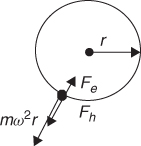
Another factor to consider in ionospheric propagation is the relative attenuation of the two magneto-ionic waves (the ordinary and extraordinary waves), which depends on the geometry of the path. This can be illustrated by considering longitudinal propagation where the two waves are circularly polarized. The forces F exerted on an electron are (i) ![]() , which is due to the electric field of the incident wave, (ii)
, which is due to the electric field of the incident wave, (ii) ![]() due to the earths' magnetic field and (iii) the centripetal force given by
due to the earths' magnetic field and (iii) the centripetal force given by ![]() ; here e and m are the charge and the mass of the electron respectively, E, is the electric field of the wave, B is the magnetic flux of the earth's field, r is the radius of gyration as illustrated in Figure 2.5 and ν is the velocity of the electron.
; here e and m are the charge and the mass of the electron respectively, E, is the electric field of the wave, B is the magnetic flux of the earth's field, r is the radius of gyration as illustrated in Figure 2.5 and ν is the velocity of the electron.
Figure 2.5 Illustration of forces on an electron in a magneto-ionic medium.
At equilibrium the ordinary wave would settle to an orbit r smaller than it would be in the absence of the magnetic field, whereas that of the extraordinary wave is larger. The increase in the radius of gyration of the extraordinary wave results in dissipation of kinetic energy when collisions occur. Consequently, the attenuation of the extraordinary wave is greater than it would be in the absence of the earth's magnetic field while that of the ordinary wave is slightly reduced.
Following [6] it is assumed that the nondeviative absorption L (dB) of the ordinary and extraordinary waves is of the form:
2.15 ![]()
where the minus sign is for the ordinary wave and the plus sign is for the extraordinary wave and fL is the longitudinal component of the gyro-frequency. Since the gyro-frequency depends on the earth's magnetic field, then for oblique propagation the up and down gyro-frequencies are different. The relationship between the absorption of the ordinary and the extraordinary waves can be derived as follows:
where X refers to the extraordinary wave, O refers to the ordinary wave, U for up leg and D for the down leg.
The total absorption of the wave is the sum of the attenuation for the up leg and down leg:
Equations (2.16) and (2.17) can be combined to give the relative attenuation of the two magneto-ionic waves as:
This can be used to predict the relative signal strength of the received waves.
2.3 Attenuation Due to Propagation into Buildings
Due to the ubiquitous nature of wireless radio systems, numerous models and measurements have been performed to estimate the excess path loss of walls of different types of buildings and penetration loss through different floors in various frequency bands. These were either direct measurements of penetration loss or measurements to obtain the properties of materials such as those listed in Table 1.2.
Recall from Equation (1.50) that for a lossy material it is the conductivity or the imaginary part of the complex permittivity ∈ that gives rise to the attenuation factor α. This means that we need to estimate ![]() at different frequencies. Alternatively, we estimate the loss tangent, which can be related to the complex part of the permittivity of Equation (1.50) as follows:
at different frequencies. Alternatively, we estimate the loss tangent, which can be related to the complex part of the permittivity of Equation (1.50) as follows:
2.19 ![]()
This can be expressed as:
2.20 ![]()
2.21 ![]()
where ![]() is the imaginary part of the complex permittivity and
is the imaginary part of the complex permittivity and ![]() is the real part of the complex permittivity.
is the real part of the complex permittivity.
For a dielectric with small loss, the tangent of the angle is approximately equal to the angle and in this case the power decays in the ratio of ![]() . In [7, p. 55] the real and imaginary parts of the complex permittivity are given for different types of material and in [8] the complex permittivity was measured for various types of wall material at 2.3 GHz and 5.25 GHz and estimates for the loss tangent were obtained as listed in Table 2.3. In addition to the loss tangent, Table 2.3 gives the transmission loss (dB). The table shows that for most wall materials the decrease in transmitted power between 2.3 GHz and 5.25 GHz is less than 1 dB, the exceptions being red brick (10.1 dB), glass (1.2 dB), 2 inch Fir lumber (3.3 dB), cinder block (3.6 dB) and stucco (which increased 1.6 dB). Stucco is concrete poured on diamond mesh orientation with a total thickness of 25.75 mm. Cinder block comprises blocks approximately 406 mm (w) by 203 mm (h) by 194 mm (d) outside dimensions, with construction as four exterior ‘walls’ and one cross member bisecting the widest dimension, with wall thickness of 31–35 mm.
. In [7, p. 55] the real and imaginary parts of the complex permittivity are given for different types of material and in [8] the complex permittivity was measured for various types of wall material at 2.3 GHz and 5.25 GHz and estimates for the loss tangent were obtained as listed in Table 2.3. In addition to the loss tangent, Table 2.3 gives the transmission loss (dB). The table shows that for most wall materials the decrease in transmitted power between 2.3 GHz and 5.25 GHz is less than 1 dB, the exceptions being red brick (10.1 dB), glass (1.2 dB), 2 inch Fir lumber (3.3 dB), cinder block (3.6 dB) and stucco (which increased 1.6 dB). Stucco is concrete poured on diamond mesh orientation with a total thickness of 25.75 mm. Cinder block comprises blocks approximately 406 mm (w) by 203 mm (h) by 194 mm (d) outside dimensions, with construction as four exterior ‘walls’ and one cross member bisecting the widest dimension, with wall thickness of 31–35 mm.
Table 2.3 Measured dielectric parameters for different building materials and corresponding transmission loss at 2.3 and 5.25 GHz [8]
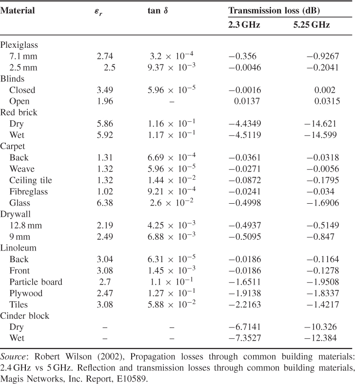
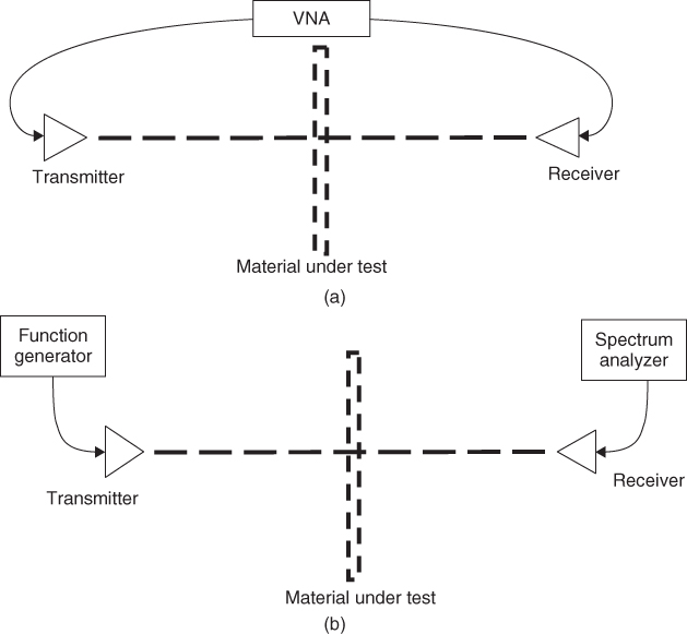
The measurements in Table 2.3 were performed in an anechoic chamber where a wall made of the building material under test is set up as illustrated in Figure 2.6. Excess path loss can then be measured from the received signal strength with and without the wall material in the propagation path. Figure 2.7a and b displays two possible measurement set-ups where the material under test is in the path of propagation where a vector network analyzer is used to measure the S21 parameter or, alternatively, a function generator feeds the transmit antenna and a spectrum analyzer measures the received signal strength.
Figure 2.6 Brick wall set up in an anechoic chamber for penetration loss measurements.
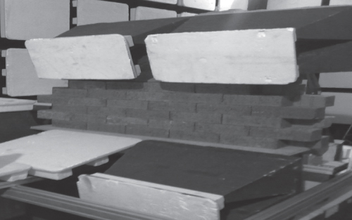
Figure 2.7 Possible configurations for measuring the penetration loss through material.
A test conducted with the configuration in Figure 2.7a in an open environment was performed at 60 GHz with highly directive horn antennas [9]. The receiver antenna was placed on a grid to obtain an average reading and the results for different types of material are listed in Table 2.4 for different transmit and receive polarizations. The table shows that, for the same thickness, an additional ∼2.5 dB loss is experienced for plywood in comparison with plastic.
Table 2.4 Transmission loss in different materials at 60 GHz [9]
| Polarization | Vertical to vertical polarization | Horizontal to horizontal polarization |
| Material | Average loss (dB) | Average loss (dB) |
| Plastic partition, 0.8 cm | 3.44 | 4.04 |
| Plywood, 0.8 cm | 6.09 | 5.42 |
| Thick wood board, 1.8 cm | 9.24 | 8.48 |
| Tempered glass, 0.7 cm | 4 | 3.97 |
Source: Huang, T.W., Lin, W.H., Lo, J.Z. et. al, IEEE 802.11-09/0995rl. 60 GHz Transmission and Reflection Measurements.
The test results presented in Tables 2.3 and 2.4 give an idea about the penetration loss for specific materials. However, buildings are constructed from a combination of different materials with different linings that modify the attenuation. Hence, measurements in real environments tend to be performed to estimate the penetration loss through buildings and between floors. Typical reported values for transmission loss through different external walls in the 1–2 GHz example are listed in Table 2.5.
Table 2.5 Penetration loss through different building materials [10, Chapter 4]
| Material | Loss (dB) |
| Porous concrete | 6.5 |
| Reinforced glass | 8 |
| Concrete (30 cm thick) | 9.5 |
| Concrete wall (25 cm) with large glazed panes | 11 |
| Thick concrete wall (25 cm) without glazed panes | 13 |
| Thick wall (>20 cm) | 15 |
| Tile | 23 |
Numerous other measurements at different frequencies in various environments have been reported. Table 2.6 presents examples of some of these results. The measurements reported in [11–21] indicate that, on average, penetration loss decreases as more sides of the building are illuminated and as the floor level increases, which is due to higher clearance from neighbouring buildings. In contrast higher losses are experienced as the number of internal partitions increases, the size of the property increases from a small villa to a mansion and the density of houses in a row increases.
Table 2.6 Penetration loss into buildings
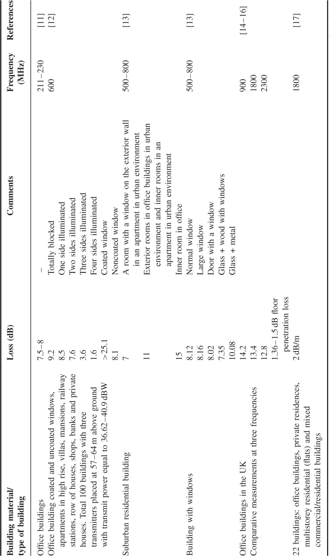
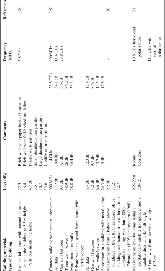
The store room with metallic shielding measured in [19] had lower penetration loss at the higher frequencies than the 900 MHz example, which was attributed to coupling through the metal and the window opening, which allowed more energy to flow to the outside of the room. Comparing the results for the concrete building in Tables 2.6 and 2.5, the 17.7 dB example is comparable with the 15 dB one obtained from the COST 231 measurements for thick walls.
2.4 Transmission Loss due to Penetration into Vehicles
Applications of radio communication links into vehicles include vehicle-to-vehicle transmission, digital video broadcasting, satellite navigation, mobile radio telephony and infotainment. Measurements of transmission loss into vehicles are reported in [22–25]. In [25], measurements at four frequencies (600, 900, 1800 and 2400 MHz) were performed with a spectrum analyzer in a minivan driven at 1–2 km/h over distances from 3 to 75 m from the transmitter. The transmitter had a vertically polarized omnidirectional antenna mounted 3 m above the ground. Similar antennas were deployed at two receivers: one outside the vehicle and a second inside the vehicle between the driver and passenger seat at about 0.6 m above the vehicle's bottom plate. The mean path loss for the different orientations, frequencies and antenna polarization with the mean loss from all the measurements shows that higher attenuation is experienced with horizontally polarized antennas and when the transmitter is illuminating the back of the vehicle. Some frequency dependence of the path loss is also observed from the results, although it does not follow a regular pattern with frequency. For example, the average of all data for both antenna polarizations is given as: 14.68, 12.4, 8.69 and 13.68 dB for the 600, 900, 1800 and 2400 MHz bands respectively. In other path loss studies of outdoor to indoor, this effect has been attributed to material properties, thickness of wall/obstruction and diffraction around the window area [26].
2.5 Diffraction Loss
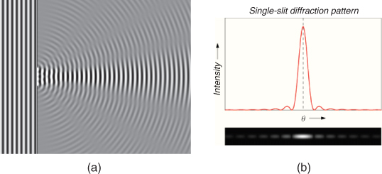
Diffraction occurs when a dense material such as hills, rooftops, lamp-posts, window openings or furniture are in the path of the illuminated area between the transmitter and receiver. Diffraction is always there becoming significant when the wavelength is comparable to the obstruction. Figure 2.8a illustrates diffraction of a wave from a slit and the summing of the diffracted wavelets on a receiving screen (Figure 2.8b). Figure 2.8 shows that, although the signal strength is strongest along the straight line through the slit, diffraction spreads the energy beyond the line of sight (LOS) path.
Figure 2.8 (a) Diffraction through a slit and (b) field intensity due to single slit diffraction.
2.5.1 Fundamentals of Diffraction Loss: Huygen's Principle
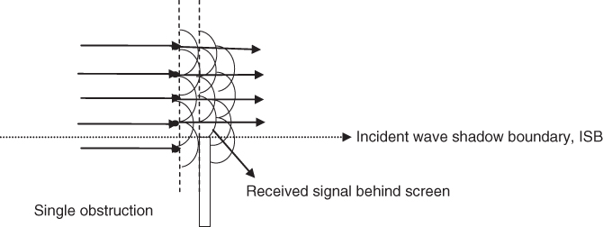
Diffraction loss may be estimated by applying Huygen's principle, which states that a well-defined obstruction to an electromagnetic force creates new wavefronts that travel into the geometric shadow of the obstruction. Each point on the wavefront acts as a source for other wavelets, as shown in Figure 2.9. Although the obstacle blocks some of the waves, the waves above the obstacle generate wavelets that propagate to the shadow area behind the obstacle. For the shown angle of incidence, the dotted line indicates the incident wave shadow boundary [7, p. 122].
Figure 2.9 Illustration of Huygen's wavelets.
2.5.2 Diffraction Loss Due to a Single Knife Edge: Fresnel Integral Approach
The loss of signal strength due to a single obstruction as in the geometry of Figure 2.10 is given by the ratio of the received electric field E, which is the sum of all the diffracted wavefronts to the free space field Eo or, alternatively, the sum of the wavefronts above the edge of the obstruction.
Figure 2.10 Path profile model for (single) knife edge diffraction.
From Huygen's principle this ratio is given by:
where ![]() is the Fresnel–Kirchoff parameter given by:
is the Fresnel–Kirchoff parameter given by:
where ![]() is the phase path difference between the direct path and the diffracted path.
is the phase path difference between the direct path and the diffracted path.
From Figure 2.10, ![]() can be related to the difference in path length
can be related to the difference in path length ![]() , which is equal to:
, which is equal to:
where ![]() . Assuming that
. Assuming that ![]() , Equation (2.24) can be simplified to:
, Equation (2.24) can be simplified to:
2.25 ![]()
where use is made of the approximation:
The range difference can be converted to a phase difference, and using the diffraction parameter defined in Equation (2.23) we obtain the phase difference equation:
2.27 ![]()
To evaluate Equation (2.22) the complex exponential is expanded into its trigonometric equivalent:
where each term in Equation (2.28) can be expressed as:
and
Equation (2.28) can then be rewritten in terms of the real part C(ν) and the imaginary part S(ν) of the Fresnel integral, given in Equation (2.30) and displayed in Figure 2.11a:
Substitution in Equation (2.22) gives the known result:
Figure 2.11 (a) C(ν) and S(ν) and (b) Cornu or Euler spiral.
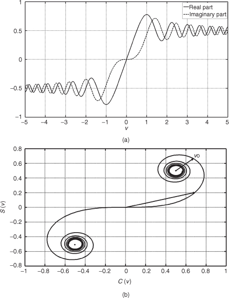
Another plot that is used for visual interpretation of the electric field strength is the Cornu or Euler spiral, which is a plot of the C(ν) versus S(ν) as in Figure 2.11b. The spiral has the property that the length of arc measured from the origin is equal to ν and that positive values of ν fall in the first quadrant while negative values of ν fall in the third quadrant. Another property of the Cornu spiral is that a line drawn from the origin to a point on the spiral (see the arrow from the origin) with a particular value of ν gives the magnitude and phase of the complex integral expressed as C(ν)–j S(ν). To use the Cornu spiral to estimate the electric field Equations (2.29a) and (2.29b) indicates that we need to displace both the real and the imaginary parts by half, as indicated in the dot placed at (1/2, 1/2). The electric field E can then be estimated by taking a line from the point at (1/2, 1/2) to the corresponding value of ν. A more practical estimation of the electric field strength can be obtained from numerical computation of Equation (2.31) as in Figure 2.12, which displays the relative field strength in dB versus the diffraction coefficient ν.
Figure 2.12 Magnitude of relative field strength versus ν.
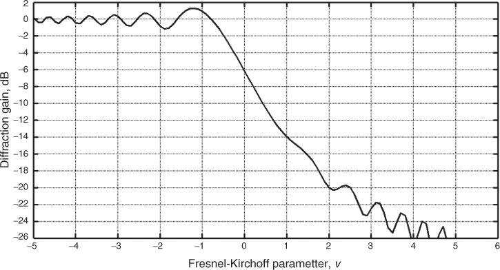
From Figure 2.12 we can deduce the following properties:
Figure 2.13 (a) Grazing angle where obstacle is directly in the LOS of the path and (b) the obstacle is below the LOS.
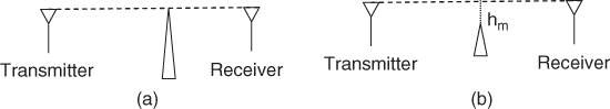
Figure 2.12 indicates that there is a need to keep some clearance distance to the first obstacle along the path between the transmitter and the receiver. The amount of this clearance is defined in terms of Fresnel zones, which are regions bounded by ellipsoids of revolution whose foci are at the transmitter and at the receiver. Recall that ellipsoids have the property that the locus of points formed by lines that connect the two foci other than the direct line have the same length as shown in Figure 2.14a. Fresnel zones correspond to the cases where the excess path length from the direct LOS is equal to multiples of λ/2 or, equivalently, to a phase difference equal to multiples of π. If a plane is drawn in the middle perpendicular to the line that connects the two foci, then the Fresnel zones can be formed from circles with radii equal to nλ/2 as is Figure 2.14b, where n is an integer. The first Fresnel zone is a disc whereas the others are rings.
Figure 2.14 Illustration of the Fresnel zones: (a) ellipsoids of the Fresnel zones and (b) radii of circles at the centre of the LOS path defining the Fresnel zones.
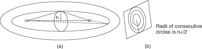
Waves within the first Fresnel zone and odd multiples of it have a similar phase orientation whereas even zones give rise to an antiphase relationship. Relating the Fresnel zones to the diffraction parameter gives the following relationship for the height of the obstruction above the direct path:
To minimize diffraction loss, it is recommended that at least 0.6 of the first Fresnel zone is cleared without any obstruction. Since the size of the Fresnel zone is frequency dependent, the higher the frequency, the smaller the size of the Fresnel zone. So for a particular geometry, higher frequencies will suffer less from diffraction loss.
2.6 Diffraction Loss Models
2.6.1 Single Knife Edge Diffraction Loss
The previous analysis gave the diffraction loss due to a single obstacle in terms of Fresnel integrals, which can then be estimated graphically by determining the diffraction parameter from Figure 2.12.
A number of alternative approximations that also use the diffraction parameters exist [27]. These include the following expressions:
Another set of approximations are those given by Lee [28]:
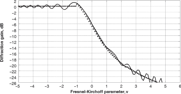
Figure 2.15 compares the Fresnel integral attenuation with both Lee's approximations and the approximation of Equation (2.33b). Close agreement is seen between the two approximations and the Fresnel equations for values of ν > −0.7. For ν <−0.7, the Fresnel equations show oscillations that decrease close to zero and can be considered negligible.
Figure 2.15 Diffraction gain as computed from the Fresnel integral (solid line) with Lee's approximate formulae (dashed line) and Equation (2.33b) (dotted line).
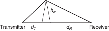
So far the transmitter and receiver heights above ground were assumed to be identical and the earth's surface was assumed to be flat. A more generalized geometry can be seen in Figure 2.16, where the transmitter and receiver heights are ht and hr respectively, the earth's bulge above the reference line that connects them is re and the height of the obstacle above ground is hm. For ![]() the height of the edge above the reference plane can be approximated by h, which can then be used in the diffraction calculation instead of hm [27]:
the height of the edge above the reference plane can be approximated by h, which can then be used in the diffraction calculation instead of hm [27]:
2.35 
Figure 2.16 Diffraction above the bulge of the earth [27]. Source: ITUR-526 Propagation by diffraction.
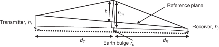
It is necessary to account for the curvature of the earth and for any slope in the path to calculate how far a knife edge impinges on a path. This is done by defining a reference plane and finding the height h of the obstacle above this reference, as illustrated in Figure 2.16. The value of h is then used to estimate the diffraction parameter.
2.6.2 Multiple Edge Diffraction Loss
Diffraction due to multiple edges is a complicated mathematical problem, which can be solved using numerical computations. Alternative approximate models commonly used to compute the diffraction loss over multiple knife edges are based on the single knife edge diffraction model using the Fresnel–Kirchoff parameter. They all have potential errors that depend on the geometry and the separation between the edges. Some of the popular models are described in this section.
- Bullington Method. In this method [29], the terrain is replaced by a single ‘equivalent’ knife edge at the point of intersection of the horizon ray from each of the terminals, as shown in Figure 2.17. The diffraction loss is then computed using Equations (2.33a), (2.33b), (2.33c) and (2.34) with the parameters for distance and height being those of the equivalent obstacle, that is (hm, dT, dR). This method has the advantage of simplicity but it generally underestimates path loss as it does not take into account other important intermediate obstacles.
- Epstein–Peterson Method. In the Epstein–Peterson method illustrated in Figure 2.18 [30], the diffraction loss is the sum of all losses due to each obstacle where, starting at the transmitter, the loss due to the first obstacle is found by assuming that obstacle 2 is the receiver taking (hm1, d1, d2) as the height and distances for the computation of diffraction parameter and diffraction loss for the first obstacle. Loss due to obstacle 2 is then found by assuming obstacle 3 as the receiver and obstacle 1 as the transmitter, with (hm2, d2, d3), and so on. The total loss is the sum of all the losses. Large errors occur when the two obstacles are closely spaced.
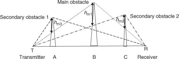
- Deygout Method. Deygout [31] suggested searching for the ‘main’ obstacle, which has the highest value of v along the path. This is done by calculating the value of the diffraction parameter for each obstacle in the absence of all other obstacles. The diffraction loss due to the main obstacle is first found. This is followed by adding the loss due to the ‘secondary’ obstacles by drawing lines between the ‘main edge’ and the transmitter and the receiver. For several obstacles, it is usual to consider only three components, the main edge and the subsidiary main edges on either side. Thus for Figure 2.19, the diffraction loss due the main obstacle is computed for (hm1, dTB, dBR), then the losses are added from secondary obstacle 1 (hm3, dTA, dAR) and secondary obstacle 2 (hm2, dTC, dCR). The Daygout method is very good in most cases. However, it overestimates the path loss when the obstructions are close together.
Figure 2.17 The Bullington ‘equivalent’ knife edge.
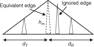
Figure 2.18 Epstein–Peterson diffraction method.
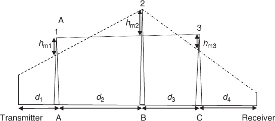
Figure 2.19 Deygout diffraction method.
2.6.2.1 Alternative Diffraction Loss Relationship
For multiple obstacles the diffraction loss can be approximated using Vigants' method [32]:
2.36 ![]()
where F1 is the radius of the first Fresnel zone in metres evaluated from Equation (2.32) by setting n = 1 and h in metres is the height of the most significant obstruction.
2.7 Path Loss Due to Scattering
When a wave is incident on a rough surface and the Rayleigh criterion ![]() is greater than 10 (Section 1.6.3), a fraction of the scattered energy reaches the receiver. To account for this loss of energy, Ament [33] introduced the scattering loss factor ρs given by:
is greater than 10 (Section 1.6.3), a fraction of the scattered energy reaches the receiver. To account for this loss of energy, Ament [33] introduced the scattering loss factor ρs given by:
2.37a ![]()
which was later modified by Boithias [34] as:
2.37b ![]()
where Io is the Bessel function of the first kind and zero order.
Another method for calculating the received scattered power is to use the radar equation where the rough surface is characterized by its radar cross section (RCS) σ in units of m2. The RCS of a target is the effective area that would scatter energy back in the direction of the receiver [35, 36] and can be used to identify various shaped objects. Assuming that the transmitted power is Pt, with antenna gain Gt and corresponding aperture A, which is related to the gain as in Equation (2.3), the received power Pr for the bistatic configuration in Figure 2.20a and for the monostatic configuration in Figure 2.20b are given by the following equations respectively:
2.38a ![]()
2.38b ![]()
Figure 2.20 Scattering of the signal in the direction of the receiver, illustrating radar cross section.
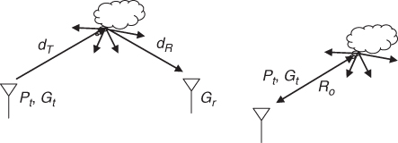
where the first term in parentheses is the power density at the reflector, which reradiates power in the direction of the receiver proportional to its cross section σ, the third term is power density at the receiver as intercepted by the antenna aperture and λ is the wavelength of the transmitted signal.
2.8 Multipath Propagation: Two-Ray Model
Reflection and refraction by dielectrics, conductors and ionized media have been discussed in detail in Chapter 1. The effect of reflection/refraction is the reception of multiple components that are delayed from each other in time and suffer different attenuations. Generally, in a built-up environment there is a large number of such components, whereas in propagation via the ionosphere, multiple components arrive due to reflections from different layers, the splitting of the two magneto-ionic waves and multiple hops between the ground and the ionosphere.
To understand the phenomenon of multipath propagation and its effects on the received signal strength, we start by studying propagation by two paths and investigate the application of the model to two special cases: (i) a LOS ray and a reflected ray from the ground, commonly known as the two-ray model in terrestrial mobile radio propagation, which gives the effect of the presence of two components as a function of distance at a particular frequency, and (ii) the interference between the two magneto-ionic waves that result from propagation via the ionosphere, referred to as polarization rotation or Faraday rotation. The interference between the two rays/components illustrates the effect of two paths as a function of distance, frequency and time. This is followed in Section 2.9 by the more general case when numerous multipath components are present.
2.8.1 Two-Ray Model in a Nondispersive Medium
Assume a simple propagation environment where two paths connect the transmitter and the receiver as shown in Figure 2.21. The received electric field due to the two paths connecting the transmitter to the receiver can be expressed as:
where Eo and E1 are the electric fields due to the first and second arriving components respectively, Δ is the phase difference due to the difference in path length ![]() or time delay difference
or time delay difference ![]() between the two components, λ is the wavelength of transmission, vp is the phase velocity in the medium, which is equal to the speed of light c in free space, and f is the frequency of the transmitted wave.
between the two components, λ is the wavelength of transmission, vp is the phase velocity in the medium, which is equal to the speed of light c in free space, and f is the frequency of the transmitted wave.
Figure 2.21 Two path propagation via two non line of sight components.
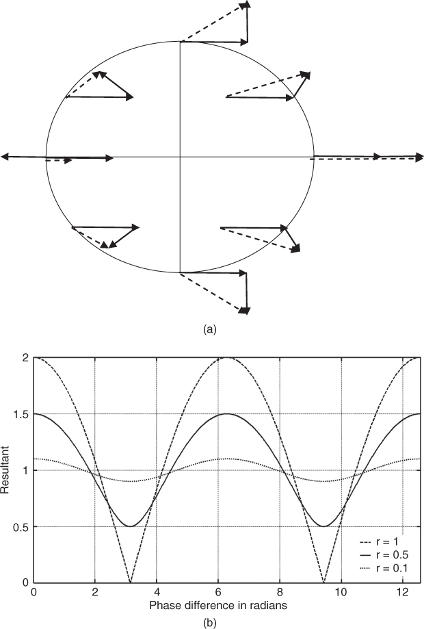
Equation (2.39) forms the basis of the two-ray propagation model and indicates that if Δ = 0 the magnitude of the received electric field is Eo (1 + ρ) and has a maximum value if ρ = 1. If Δ = 180° the resultant has a minimum value equal to Eo (1 – ρ), which can be equal to zero if ρ = 1. For all other values of Δ, the resultant has a value between these two limits and it will go through maxima and minima as Δ varies between 0 and 360°, as illustrated in Figure 2.22 both as a phasor summation around 360° and the magnitude as a function of phase difference. The figure shows that the separation between any two adjacent maxima or any two adjacent minima is equal to 2π radians, which corresponds to a wavelength spatial separation between the two paths. The change in the spatial separation between the two paths can occur either due to the movement of the transmitter or receiver and/or due to the movement of the reflector such as, for example, a path being reflected from a vehicle. These variations are normally referred to as time variations. To distinguish the effect due to the time movement from the spatial effect of the multipath components, we assume a totally stationary environment. Keeping the transmitter fixed and probing the electric field at different points in space, the received signal will vary as in Figure 2.22 along the path giving rise to ‘spatial’ variability. Thus the presence of the two rays gives rise to signal strength variations in space that the receiver samples at it moves in space. Equation (2.39) also indicates that a change in frequency which corresponds to ![]() also gives rise to maxima and minima as in Figure 2.22. This type of variation is referred to as frequency selectivity. The effects illustrated in Figure 2.22 are experienced over a fraction of a wavelength and are thus referred to as ‘small-scale’ variations, which are distinct from variations in the received signal strength when the separation between the two terminals varies over large distances. The latter is referred to as ‘large scale’ variations and will be discussed below in the plane earth model.
also gives rise to maxima and minima as in Figure 2.22. This type of variation is referred to as frequency selectivity. The effects illustrated in Figure 2.22 are experienced over a fraction of a wavelength and are thus referred to as ‘small-scale’ variations, which are distinct from variations in the received signal strength when the separation between the two terminals varies over large distances. The latter is referred to as ‘large scale’ variations and will be discussed below in the plane earth model.
Figure 2.22 (a) Phase representation of two multipath components and their resultant and (b) signal strength variations as a function of phase rotation for different values of r = ρ.
2.8.2 Two-Ray Model due to LOS and Ground Reflected Wave: Plane Earth Model
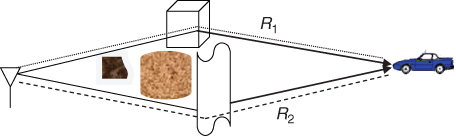
Figure 2.23 displays the geometry for the two-ray model commonly used in mobile radio propagation studies. This model is used to estimate path loss in environments where there is a likelihood of few obstructions between the transmitter and receiver, and no foliage. In this case the received electric field strength in Equation (2.39) consists of the direct free space wave Eo and the reflected wave E1, where ρ is the reflection coefficient of the earth and Δ is the phase difference between the direct path and the ground-reflected wave. Considering Figure 2.23, the phase difference Δ is proportional to R2 − R1.
Figure 2.23 Geometry for the two-ray model.
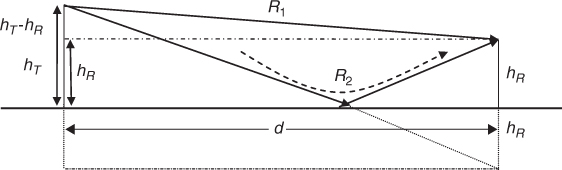
Assuming that the distances between the transmitter and receiver ![]() and using the approximation in Equation (2.26)
and using the approximation in Equation (2.26) ![]() , expressions for R1 and R2 can be found to be:
, expressions for R1 and R2 can be found to be:

Using Equations (2.40a) and (2.40b) reduces the difference ΔR = R2 − R1 to:
2.41 ![]()
giving a phase difference that can be expressed as:
For grazing incidence, that is when the angle of incidence on earth is very small or equivalently θi = 90°, Equations (1.85) and (1.89) indicate that the reflection coefficient ρ⊥ tends to −1 and ρ|| = 1, so the received electric field can be expressed as:
2.43 ![]()
Thus the magnitude of the electric field is:
2.44 
The received power is proportional to |E|2; hence for a vertically polarized wave:
Equation (2.45) indicates an oscillatory nature for the received power. However, for propagation distances that substantially extend beyond the turnover point ![]() , that is for values of
, that is for values of ![]() , Equation (2.45) tends to the fourth power distance law given by:
, Equation (2.45) tends to the fourth power distance law given by:
The expression in Equation (2.46b) is known as the plane earth propagation equation and differs in two important ways from the free space equation in Equation (2.6). Firstly, it is frequency independent and, secondly, it obeys a fourth order power law with range; that is the received power decreases more rapidly with range at 12 dB/octave instead of 6 dB/octave. In logarithmic form, Equation (2.46b) can be written as:
2.47 ![]()
Figure 2.24 displays the properties of the two-ray model assuming that the transmit power is 500 W, the transmit frequencies are 900 MHz and 1800 MHz and the transmitter and receiver antenna heights are 100 m and 8 m above ground respectively. Superimposed on the plots, the free space received power line obeys a second order power relationship with distance as in Equation (2.6) and the fourth order power relationship as in Equations (2.46a) and (2.46b). The following observations can be made from the figure: (a) the frequency dependence on free space is shown to be 6 dB/octave, (b) the frequency dependence of the two-ray model in the regions governed by oscillations and (c) the received signal falls off initially at the second order power relationship, that is d2, and then at the fourth order power relationship d4, as indicated by the circles at the intersections. The intersection point is often called the Fresnel breakpoint and represents the point where the ground starts to enter into the first Fresnel zone, which from Equations (2.32) and (2.42) occurs at ![]() .
.
Figure 2.24 Two-ray model comparison with the free space model at 900 and 1800 MHz.
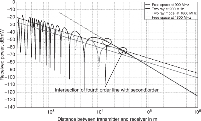
The maxima and minima in Figure 2.24 represent multipath interference between the two rays as they add in phase and out of phase as a function of distance. Comparing the plots for the two frequencies, the 1800 MHz displays two peaks and a minimum for each corresponding 900 MHz peak.
In communication systems that extend over ranges in excess of 30 km, the signal strength can be thought of as falling off at a rate of d4. For antenna heights more typical of short range coverage area the approximation in Equation (2.46) is inappropriate and the full wave equation needs to be taken into account. For an electric field in a general direction r, the received power can be written as [37]:
2.48 ![]()
and ρ is given either by Equations (1.85) or (1.89) for vertical or horizontal polarization respectively.
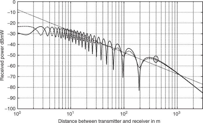
Assuming 1 W of transmitted power with isotropic antennas, low antenna heights of 10 and 1.6 m and using similar parameters as in [37, Figure 3], for average ground conductivity of 0.005 and relative permittivity of ![]() , the received power is displayed in Figure 2.25. The figure displays the results for both horizontal polarization (dotted line curve) and vertical polarization (solid line curve) at 1800 MHz transmission frequency, with the dotted line showing the free space slope of 1/d2. Here the breakpoint indicated by a circle on the figure is seen to occur at a closer range on the order of a few hundred metres in contrast to tens of kilometres for the example of Figure 2.24.
, the received power is displayed in Figure 2.25. The figure displays the results for both horizontal polarization (dotted line curve) and vertical polarization (solid line curve) at 1800 MHz transmission frequency, with the dotted line showing the free space slope of 1/d2. Here the breakpoint indicated by a circle on the figure is seen to occur at a closer range on the order of a few hundred metres in contrast to tens of kilometres for the example of Figure 2.24.
Figure 2.25 Received power for 1800 MHz signal for both horizontal (dashed line) and vertical (solid line).
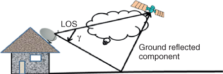
Another application of the two-ray model is shown in Figure 2.26 between a ground station and an airborne satellite where the first component is the LOS component that suffers from atmospheric impairment and the second component is a ground-reflected wave that also suffers from impairment [38]. The model assumes a hilly terrain and estimates the fade depth, that is the value of the minima versus clearance angle, which is the angle between the ray from the transmit antenna to the ground and the LOS ray to the airborne satellite. Approximate expressions for the fade depth for vertically and horizontally polarized waves are given as ![]() , where γ is the clearance angle.
, where γ is the clearance angle.
Figure 2.26 Two-ray model for an airborne communication link.
Generally speaking, depending on the frequency, it might be necessary to combine the two-ray model with other losses such as atmospheric losses.
2.8.3 Two-Ray Propagation via the Ionosphere
As discussed in Section 1.7.2, when a linearly polarized wave is incident on the ionosphere it splits into two components, the ordinary wave and the extraordinary wave, which travel over different path lengths and suffer different attenuation, as expressed in Equation (2.18). On exit from the ionosphere they combine to give an elliptically polarized wave with an angular rotation given by Jordan and Balmain [39, p. 693]:
where
e and m = charge and mass of an electron respectively
Bo = earth's magnetic field
c = speed of light
N = electron density
Ω = angular frequency (rad/s)
z = distance travelled in the medium; and
ϵv = σ/ω![]() , where σ is the conductivity and
, where σ is the conductivity and ![]() is the complex part of the relative permittivity
is the complex part of the relative permittivity
A linearly polarized antenna will pick the component along its axis of polarization. As the frequency of propagation varies, Equation (2.49) indicates that the tilt angle will also vary, giving rise to variations in the received signal strength as a function of frequency. This phenomenon is known as Faraday rotation, and is observed for each propagation path, for example the 1F1, 1F2 or 1E layer.
The effect of Faraday rotation can be studied by isolating a particular propagation path, say the 1F2 path shown in Figure 2.27. The ionogram displays the two magneto-ionic waves as a function of frequency in a 4 MHz transmission bandwidth (4.88–8.88 MHz) over a 270 km link in the UK [40]. The two magneto-ionic waves are seen to merge around 6.5 MHz and split after 6.9 MHz. The relative amplitude and time delay separation between the two waves varies with frequency with the extraordinary wave persisting over a higher frequency range.
Figure 2.27 Ionogram over a 270 km link in the UK displaying the two magneto-ionic waves for 1F2.
The ionogram shows that as the two magneto-ionic waves travel over different paths, they have different times of travel as the frequency changes or, equivalently, the time delay difference ![]() is a function of frequency. This is in contrast to a nondispersive medium where the time delay difference
is a function of frequency. This is in contrast to a nondispersive medium where the time delay difference ![]() is independent of frequency.
is independent of frequency.
For a narrowband HF system, the two waves combine to give a resultant that depends on their relative amplitudes and their relative phase time delay or phase delay, ![]() , where i is either o or x for the ordinary and extraordinary waves respectively. Thus the received signal can be expressed as:
, where i is either o or x for the ordinary and extraordinary waves respectively. Thus the received signal can be expressed as:
For equal amplitudes of the two waves, the resultant can be written as:
Equation (2.51) shows that at a particular instant in time, the resultant signal is amplitude modulated with frequency and time by a sinusoid, which is a function of the phase difference between the two waves. Since the two waves travel over different paths that vary with frequency, the phase difference ![]() also varies with frequency and time. For a time-invariant ionosphere the phase difference is only a function of frequency, giving rise to maxima and minima along the frequency axis as shown in Figure 2.28a.
also varies with frequency and time. For a time-invariant ionosphere the phase difference is only a function of frequency, giving rise to maxima and minima along the frequency axis as shown in Figure 2.28a.
Figure 2.28 (a) Amplitude variations with frequency and (b) polarization bandwidth.
Taking any single frequency, the envelope of the signal as in Equation (2.51) ![]() varies with time, giving rise to maxima and minima, and the
varies with time, giving rise to maxima and minima, and the ![]() also changes with time, resulting in a change in the carrier frequency, given by:
also changes with time, resulting in a change in the carrier frequency, given by:
where p0 and px are the phase path lengths of the ordinary and extraordinary waves and ![]() are the corresponding frequency shift of each component known as the Doppler shift.
are the corresponding frequency shift of each component known as the Doppler shift.
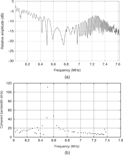
Due to the variations in the relative amplitude of the two waves and the variations of their relative phase delay as a function of frequency the depth of the minima and their frequency separation varies with frequency. This has given rise to the definition of polarization bandwidth [41], which refers to half the separation between the minima as a function of frequency. Relating Figure 2.28 to Figure 2.27, it is seen that the depth of the minima relative to the local maxima is fairly shallow over the frequency range 6.01 up to 6.4 MHz, where the ordinary wave is significantly stronger than the extraordinary wave. As the relative strength of the two components becomes comparable, the depth of the minima relative to the local maxima increases significantly. The separation between minima as a function of frequency increases as the two magneto-ionic waves get closer together and then decreases as they separate farther apart, giving rise to a small polarization bandwidth as displayed in Figure 2.28b.
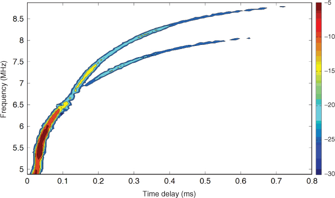
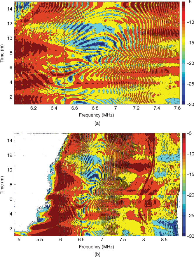
Since the electron density profile in the ionosphere varies with time of day and season, the height of reflection versus frequency changes with time, giving the time variations in the phase of the carrier and the phase difference in Equation (2.51). This results in the movement of the minima across the frequency band of transmission as seen in Figure 2.29, which displays the interference pattern between the two magneto-ionic waves as a function of time and frequency. Observing the 7–7.6 MHz frequency range in Figure 2.29a, the fading pattern cannot always be followed as a function of time due to undersampling. The blocking of the 1F2 layer by the sporadic E layer is illustrated in Figure 2.29b, which displays the entire frequency range from 4.88 to 8.88 MHz. Similar effects can be observed due to the movement of either the transmitter or the receiver.
Figure 2.29 Frequency selectivity and time fading due to interference between the two magneto-ionic waves: (a) frequency range 6–7.6 MHz and (b) 4.88–8.88 MHz.
2.9 General Multipath Propagation
In Section 2.8, we discussed the effect of interference of two waves versus frequency, distance and time. In general more than two components are received that result in a more complex interference pattern. The number of multipath components depends on the frequency band, the medium of transmission and the environment.
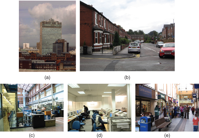
For the example of the ionosphere, multipath occurs due to reflections from multiple layers such as the 1F2, 2F2 and Es, and reflections between layers such as the M and N modes in Figure 1.22. In terrestrial communication, multipath propagation results from the presence of fixed man-made structures such as buildings, bridges, tunnels or natural terrain such as hills, mountains, trees and foliage or from moving vehicles, trains, trams or people, as in Figure 2.30. Due to the significant number of such structures a user on the street, in a factory space, in a large room or in a shopping mall will receive a large number of multipath components due to reflection, scattering, diffraction and refraction, in addition to a LOS component, if present. Depending on the presence or absence of the direct path, in wireless propagation studies the two situations are distinguished as LOS and non line of sight (NLOS), respectively.
Figure 2.30 Typical outdoor and indoor environments: (a) dense urban city [42]. Source: Salous, S., Gokalp, H., Dual frequency division duplex sounder for UMTS frequency division duplex channels. IEE Proc. Commun. Vol. 149, No. 2, April 2002, pp 117–122. Reproduced with permission of IET. (b) suburban neighbourhood, (c) factory-like indoor environment [43], (d) office-like indoor environment [43]. Source: Salous, S., Hinostroza, V., Wideband indoor frequency agile channel sounder and measurements. IEE Proc. -Microw. Antennas Propag., Vol. 152, No. 6. Reproduced with permission of IET. (e) shopping mall environment.
In this section, the main effects of multipath propagation, which include time dispersion and frequency dispersion, are discussed in relation to propagation via the ionosphere and in the UHF band in built-up areas and in indoor environments. Coherence functions that include time, frequency and space commonly used to describe the multipath effects are introduced, as well as basic fading parameters such as the level crossing rate (LCR) and average fade duration (AFD).
2.9.1 Time Dispersion due to Multipath Propagation
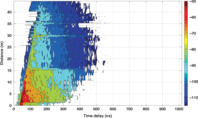
Time dispersion relates to the basic effect of multipath where a narrow transmitted pulse instead of being received as a single pulse will be received as multiple pulses dispersed in time as shown in Figure 2.31 for an indoor environment at 2 GHz. The extent of time dispersion varies for different environments and media of transmission. It can vary over small distances of travel and with time of transmission. For an example of the indoor environment of Figure 2.30c the variations of multipath dispersion as a function of spatial movement is displayed in Figure 2.32, where several effects can be observed. These include variations in the time of arrival of the first component from location to location, signal strength variations and variations in the extent of the multipath components.
Figure 2.31 Multipath propagation in an indoor environment.
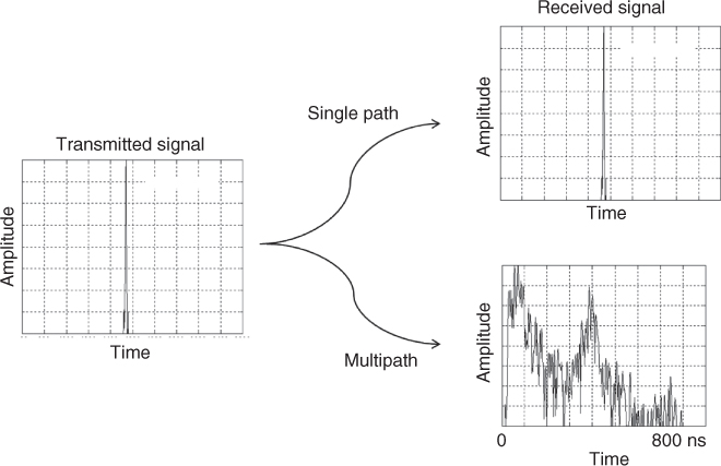
Figure 2.32 Time delay dispersion as a function of space [43]. Source: Salous, S., Hinostroza, V., Wideband indoor frequency agile channel sounder and measurements. IEE Proc. -Microw. Antennas Propag., Vol. 152, No. 6. Reproduced with permission of IET.
Time variability of a multipath for a fixed transmitter and receiver is illustrated in Figure 2.33 for two ionograms obtained in July over the frequency range 4.88–7.88 MHz, over a 270 km skywave link in the UK [40]. The ionograms are within a 6 minute observation time and show significant changes in the structure of multipath reflections from the different layers of the ionosphere. In Figure 2.33a both Es and 1F2 reflections are present up to 6.5 MHz, where thereafter only the 1F2 component is received. In the frequency range 4.88–5 MHz, the extraordinary wave from the 1F1 mode is also received. The time delay separation between the Es echo and the 1F2 echo varies between 1.2 and 1.5 ms and the two magneto-ionic waves for 1F2 are not discernable between 5 MHz and 6.5 MHz, where they subsequently split with the ordinary wave being absorbed beyond 7.5 MHz. In Figure 2.33b the sporadic E layer has receded to 6 MHz and the splitting of the two magneto-ionic waves of the 1F2 layer can now be seen between 6.2 MHz and 7.2 MHz as they come closer together and then separate again.
Figure 2.33 Ionograms over a short skywave link separated by a 6 minute observation time.
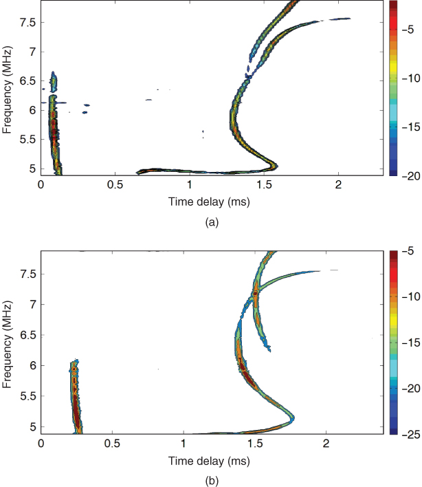
Comparing Figures 2.32 and 2.33, significant differences in the extent of time dispersion between the two propagation media of transmission are observed, where in the indoor environment the multipath structure extends up to ∼500 ns whereas for skywave propagation via the ionosphere it can be on the order of several milliseconds.
This effect is detrimental to digital data transmission. Time-dispersion results in intersymbol interference where the multiple paths received from the first data bit can overlap with the next data bit if transmitted before all the multiple paths have diminished. This effect limits the data rate of transmission in the HF band to a few kbps whereas achievable data rates are on the order of a few Mbps in the UHF band and can be up to 1 Gbps in the 60 GHz band.
Due to the time and spatial variability of multipath propagation, statistical descriptors are usually used to relate the time delay dispersion effects to the data rate. These will be discussed in detail in Chapter 3.
2.9.2 Effects of Multipath Propagation in Frequency, Time and Space
In Section 2.8.1, frequency selectivity was introduced with respect to the two-ray model. However, as seen from Figures 2.32 and 2.33, the multipath structure is far more complicated. In this section we will discuss spatial and time fading and frequency selectivity due to multipath propagation for both narrowband signals and wideband signals. In the narrowband case we will assume that, at any one time, only a single CW signal is transmitted and then consider the effect of varying the frequency of transmission. In the wideband case we will consider the transmission of a narrow pulse at a given carrier frequency and then vary the carrier frequency.
2.9.2.1 Narrowband Case: CW Signal
For a large number of multipath components, N, the received signal can be expressed as:
This is similar to Equation (2.50) where the sum is extended over N components; that is the received signal will consist of the sum of delayed replicas where each component will have its amplitude ![]() and phase shift
and phase shift ![]() , which can be frequency and time dependent. In Equation (2.52) the change in path length with time was shown to give rise to a Doppler shift and hence the received signal can be considered as the weighted sum of Doppler shifted sinusoids.
, which can be frequency and time dependent. In Equation (2.52) the change in path length with time was shown to give rise to a Doppler shift and hence the received signal can be considered as the weighted sum of Doppler shifted sinusoids.
In ionospheric propagation both the amplitude and phase delay vary with frequency and time, whereas in the UHF band it is generally assumed that they are frequency independent. Assuming UHF propagation to illustrate the concept and using phasor summation, the multipath components combine to give a particular resultant at the given frequency. By varying the carrier frequency at a particular instant in time to, the phase shift ![]() between the different multipath components varies, which gives a different resultant. If the two frequencies are sufficiently close, the resultant remains similar to that at the first frequency, which is referred to as ‘flat fading’. As the frequency separation increases, the variations in the phase shift
between the different multipath components varies, which gives a different resultant. If the two frequencies are sufficiently close, the resultant remains similar to that at the first frequency, which is referred to as ‘flat fading’. As the frequency separation increases, the variations in the phase shift ![]() between the components increase and the two resultants can be significantly different. This gives rise to maxima and minima as a function of frequency. By repeating the estimate of Equation (2.53) at different points in space, the frequency selective pattern is seen to change as the phase relationship between the different multipath components varies due to a change in the path length
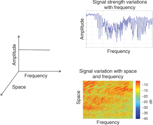
between the components increase and the two resultants can be significantly different. This gives rise to maxima and minima as a function of frequency. By repeating the estimate of Equation (2.53) at different points in space, the frequency selective pattern is seen to change as the phase relationship between the different multipath components varies due to a change in the path length ![]() and variations in their relative amplitude due to obstructions in the environment. These effects are illustrated in Figure 2.34, where a constant amplitude signal has been transmitted across the desired frequency range and the corresponding received signal versus frequency at one location and then at a number of locations. These spatial variations are commonly referred to as time fading or simply fading, since it is usually assumed that it results from the movement of the user in space as a function of time, which gives a time-variant path length
and variations in their relative amplitude due to obstructions in the environment. These effects are illustrated in Figure 2.34, where a constant amplitude signal has been transmitted across the desired frequency range and the corresponding received signal versus frequency at one location and then at a number of locations. These spatial variations are commonly referred to as time fading or simply fading, since it is usually assumed that it results from the movement of the user in space as a function of time, which gives a time-variant path length ![]() . However, the interference between the multipath components gives the spatial variations and it is by moving in space that these spatial variations are experienced. Time variability can also be observed if the two terminals are fixed and the medium of transmission moves with time, for example movement of the reflecting layer in the ionosphere or movement of a vehicle or a pedestrian in the path of the two terminals.
. However, the interference between the multipath components gives the spatial variations and it is by moving in space that these spatial variations are experienced. Time variability can also be observed if the two terminals are fixed and the medium of transmission moves with time, for example movement of the reflecting layer in the ionosphere or movement of a vehicle or a pedestrian in the path of the two terminals.
Figure 2.34 Signal strength variations in space and frequency for a single location (top right) and for consecutive locations (bottom right).
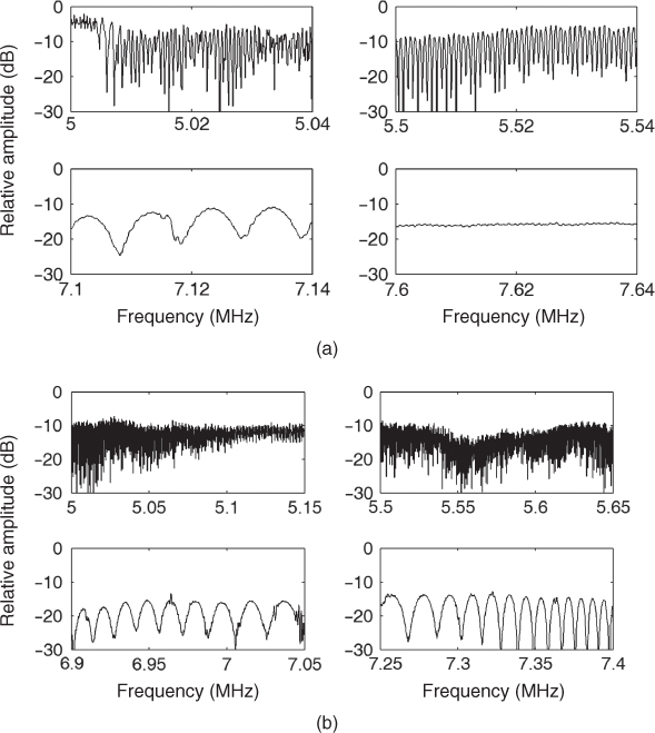
Consider now propagation via the ionosphere where the number of multipath components, their amplitude and their time delay vary with frequency. Similar to the case of UHF propagation, frequency selectivity would also arise as shown in Figure 2.35a,b, which corresponds to the ionograms of Figure 2.33a,b respectively. Considering the frequency pattern in Figure 2.35a we see that the received signal versus frequency has a variable interference pattern where the separation between the minima changes from being very small over the frequency range up to 6.5 MHz, which can be attributed to the interference between the Es layer component with the F layer component, to a considerably larger value between 6.5 MHz and 7.5 MHz, which is only due to the interference between the two magneto-ionic waves of the 1F2 layer, and then the received signal becomes flat between 7.5 MHz and 7.88 MHz when a single multipath component is received. The figure shows that as the time delay separation between the components increases, the separation between the minima decreases as discussed in Section 2.8.1. Similar comments can be made with regard to Figure 2.35b in relation to the ionogram of Figure 2.33b, where the spacing between minima can be related to the time delay separation between the two dominant multipath components. In this case, the sporadic E component contributes to the small separation between minima and as the two magneto-ionic waves of the 1F2 layer split and then come close and move apart again, the separation between the minima decreases and then increases again. Figure 2.35 illustrates that in the presence of several multipath components and due to the random nature of the time variations of the electron density of the different layers, the separation between the minima varies considerably with frequency and time for a stationary user.
Figure 2.35 Frequency selectivity in the ionosphere: (a) ionogram in Figure 2.33a and (b) ionogram in Figure 2.33b.
The HF and UHF examples presented in this section show that although the frequency selectivity illustrated in Figures 2.34 and 2.35 resulted from propagation via different media and from different multipath structures, both types of transmission indicate the need to define the following three important coherence parameters over which the signal strength remains similar or ‘flat’. These are the coherence bandwidth, the coherence time and the coherence distance. Due to the random nature of multipath propagation, these parameters require a statistical estimate that is obtained from consecutive measurements over a wide range of frequencies in space and in time such as those in Figure 2.34. The consecutive time delay responses are obtained at a rate commensurate with the rate of change of the signal in space or in time such that the sampling theorem is satisfied. Correlation analysis is then applied to the data to estimate the coherence parameters as discussed in Section 3.6.
2.9.2.2 Level Crossing Rate and Average Fade Duration
Since the received signal experiences maxima and minima as a function of time or space, it is relevant to identify a measure of the number of minima that the receiver experiences either per wavelength of displacement or per unit time. As the frequency increases, a small change in time delay results in a significant change in phase shift. For example, at 1 GHz carrier, a change in time delay of 1 ns or a change in distance of 30 cm changes the phase by 2π radians. When several components are present, these changes are random and the resultant signal experiences rapid changes as a function of time or travelled distance. Due to the high rate of change and the small distances over which it occurs this type of signal variation is called ‘fast fading’ or ‘small-scale’ variations, which are experienced by movements on the order of a fraction of a wavelength. To characterize these effects Equation (2.53) can be rewritten as:
2.54 
When N is large and if the components can be considered to be independent, the resultant envelope r(t) can be modelled by a Rayleigh distribution for short distances over which the mean level can be considered a constant and the phase ![]() is modelled with a uniform distribution.
is modelled with a uniform distribution.
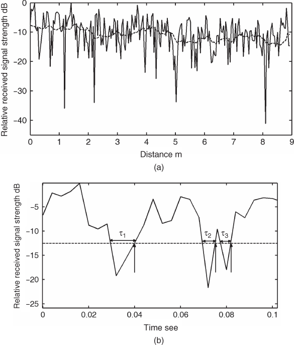
Figure 2.36a shows that relative received signal variations in excess of 40 dB are observed over a travel distance of 9 m. The average received signal strength (dashed line) obtained from averaging every 4.7λ is seen to have smaller variations ∼10.5 dB. The number of times the received signal crosses a particular level, referred at the level crossing rate (LCR), and the duration of time it spends below a specified level, called the average fade duration (AFD) is an important measure in the design of communication systems. Figure 2.36b illustrates the definition of both LCR and AFD where the double arrows indicate the time that the signal remains below the specified level of −12.5 dB and the vertical arrows indicate the times at which the specified level is crossed where either positive going crossings or negative going crossings are counted. In Figure 2.36b the distance has been converted into time using the speed of travel.
Figure 2.36 Fading as a function of (a) distance and (b) time. The vertical arrows indicate the level crossing points and the double arrows indicate the duration over which the signal fades below the threshold.
The LCR and AFD are first order statistics. LCR at any specified level R is defined as the expected rate at which the envelope, normalized with respect to the local root mean square (RMS) signal level RRMS, crosses that level in a positive going (or negative going) direction per second. Figure 2.37 gives an example of the LCR in a 1 second time interval at a carrier frequency of 1950 MHz. Similar to Figure 2.36 the data are normalized with respect to the maximum received signal and the level along the x axis gives a relative fade depth.
Figure 2.37 Level crossing rate for a CW signal.
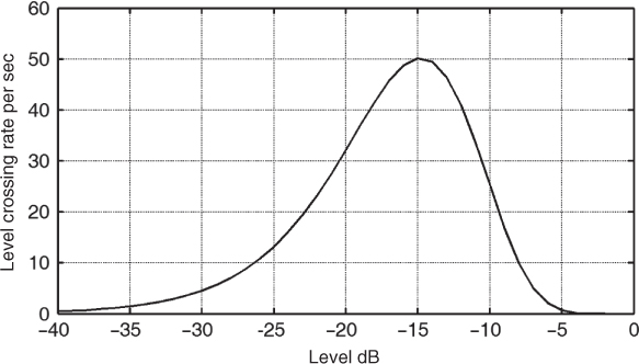
For a Rayleigh distribution (see Appendix A.1), the expected (average) crossing rate at a level R is given by:
where fm is the maximum Doppler shift and ![]() is the mean square value [44, Chapter 1]. Equation (2.55) gives NR in terms of the average number of crossings per second, where the mobile speed is inherent in the Doppler shift fm. Since the number of crossings experienced depends on how fast one drives through the spatial minima/maxima dividing Equation (2.55) by fm gives the number of level crossings per wavelength.
is the mean square value [44, Chapter 1]. Equation (2.55) gives NR in terms of the average number of crossings per second, where the mobile speed is inherent in the Doppler shift fm. Since the number of crossings experienced depends on how fast one drives through the spatial minima/maxima dividing Equation (2.55) by fm gives the number of level crossings per wavelength.
The AFD gives the average period of a fade below a specified level R. Referring to Figure 2.36b this corresponds to the mean of τi with respect to the total time of observation. For a Rayleigh distribution it is given by:
2.56 ![]()
Another parameter that is related to the AFD is the average nonfade duration (ANFD). This is useful for a communication system where a fade margin M can be defined with respect to the local mean. In a Rayleigh fading channel the ANFD is given by:
2.57 ![]()
where fm is the maximum Doppler spread and M is the ratio of the local mean signal power and the minimum (threshold) power needed for reliable communication. For example, for a GSM (Global System for Mobile Communications, formerly Groupe Spécial Mobile) system operating at 1.8 GHz, with a data rate of 1 Mbps and a vehicle travelling at a speed of 36 km/h (10 m/s giving 60 Hz Doppler shift) a packet consisting of 500 kb would need 0.5 second to be transmitted. To ensure no drop-outs in the data, the fade margin is required to be 37.6 dB!
Note that the LCR, AFD and ANFD are proportional to the speed of the terminal as they are all time-related parameters. Channel fading occurs due to the time variations, which are either due to the movement of the user or due to changes in the environment such as the movement of reflectors.
2.9.2.3 Level Crossing Frequency and Average Fade Bandwidth
The LCR and AFD are estimated from CW measurements and a high sampling rate as a function of distance/time. Over short intervals, normally referred to as small-scale variations, they can also be estimated from the time frequency function of a wideband transmission. For the example of the time frequency function in Figure 2.38a the data can be analyzed in two domains: time and frequency. By taking a vertical slice, the fading at a particular frequency can be obtained and analyzed to estimate the time fading parameters LCR and AFD. Alternatively, by taking a horizontal slice, the variations as a function of frequency can be obtained. Hence, it is possible to define frequency counterparts to the time/space fading parameters. To differentiate these from the time domain descriptors these are defined as the level crossing frequency (LCF) and the average fade bandwidth (AFBW) [45]. These parameters are important for multicarrier transmissions such as orthogonal frequency division multiplexing (OFDM) where the data stream is divided into lower data rate blocks and transmitted on multiple carriers. Figure 2.38b gives the LCF as obtained from the data in Figure 2.38a where the solid lines refer to the centre frequency of transmission, that is a single slice, and the dashed line refers to the average obtained from all the frequencies in the band. The time frequency measurement represents 2000 frequencies and 250 time samples. Figure 2.38c gives the corresponding AFBW. Taking the average across the 250 time samples or across the 2000 frequency samples gives a similar result, but with a difference in the standard deviation as shown in Figure 2.38d.
Figure 2.38 (a) Short term time and frequency variations of received signal strength, (b) level crossing rate at centre frequency of transmission (solid line) and from the average over the 2000 frequencies, (c) percentage of average fade bandwidth and (d) standard deviation of average fade duration (solid line) and average fade bandwidth (dashed line).
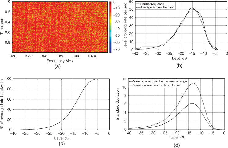
2.9.2.4 Wideband Case: Narrow Pulse Transmission
To study the effects of multipath on wideband signals we will consider two cases. The first case assumes the transmission of a periodic pulse sufficiently narrow to resolve all the received multipath components in time delay and in Doppler shift. In this case the received signal due to a transmitted pulse at a particular frequency, ![]() , can be expressed as:
, can be expressed as:
where ![]() .
.
Equation (2.58) shows that the received signal consists of the weighted sum of delayed pulses each with its own Doppler shifted carrier as shown in Figure 2.39. The figure shows that at any particular time delay a number of components might be present and if unresolved the received signal is broken down into several terms where each term is the sum of a fraction of the unresolved multipath components, given by:
2.59 
where ![]() .
.
Figure 2.39 Multipath structure in a time-variant environment.
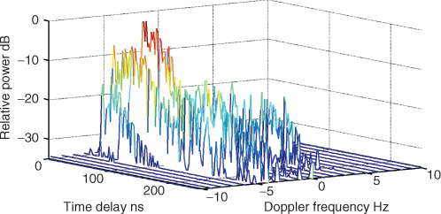
As in the case of narrowband transmission these unresolved multipath components will add to give a resultant that is dependent on carrier frequency and time of transmission. This effect can be seen in Figure 2.40, which displays the multipath structure for a 40 ns pulse transmitted across a 300 MHz bandwidth in the 2 GHz band. By varying the carrier frequency of the pulse, the multipath components combine to give different resultants.
Figure 2.40 Multipath structure as a function of frequency for a 40 ns pulse.
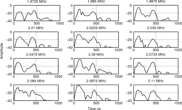
The effect of frequency selectivity on wideband signals is particularly important for communication systems that use frequency division duplex (FDD) where one frequency band is used for transmission and another for reception. The difference in the multipath structure for the FDD bands of third generation mobile phones (UMTS, or universal mobile telecommunication system) is shown in Figure 2.41, where the uplink and downlink frequencies are separated by 190 MHz. Figure 2.41a displays the multipath structure for 16.7 ns pulses and Figure 2.41b for 200 ns pulses swept across a 60 MHz bandwidth with 5 MHz increments, where the multipath structure is seen to vary with frequency within the 60 MHz band for either the uplink or the downlink and between the two FDD links.
Figure 2.41 Frequency selectivity of the uplink and downlink of the UMTS band (a) with a 16.7 ns time delay resolution and (b) with a 200 ns time delay resolution [46]. Source: Salous, S., and H. Gokalp, (2007), Medium and large scale characterisation of UMTS allocated frequency division duplex channels, IEEE Transaction on Vehicular Technology, 56(5), pp 2831-2843. Reproduced with permission IEEE.
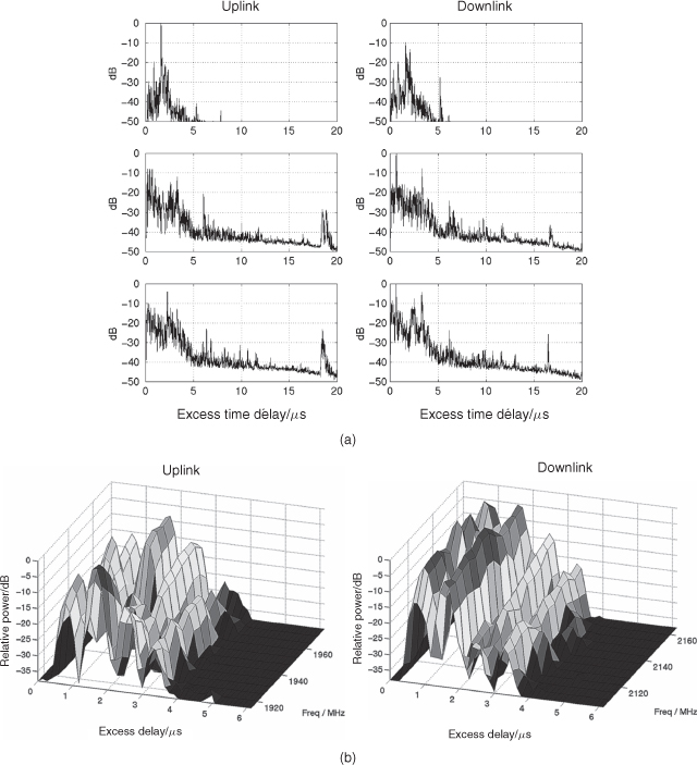
2.10 Shadow Fading: Medium Scale
So far we have examined two types of signal variations. The first is known as large-scale variation, which refers to the path loss due to the separation between the transmitter and the receiver over a large distance, and the second is due to the presence of multipath, which results in maxima and minima that are experienced over short distances of travel or short time intervals, small-scale variations. A third type of signal variation is experienced by a mobile radio user due to a change in the environment, for example when moving from a radial street to a circumferential street or a change in the height of the surrounding buildings, which might obstruct the received signal or variations in the terrain. Since this type of signal strength variation is related to the change in the environment that is experienced at a slow rate of change it is termed slow fading or shadow fading. These variations are estimated by taking measurements around a circular area from the transmitter. This isolates the effect of path loss as a function of range as all the measurements are taken at the same distance. When the received signal strength is measured in decibels its standard deviation as it moves between the different environments is referred to as location variability and in cities this is usually in the range 6–10 dB. Location variability measurements are carried out in a variety of street orientations, radial and circumferential. For example, in the measurements reported by Ibrahim and Parsons, the measurements were carried out over 500 m × 500 m sectors at 2, 5 and 9 km at 168 MHz, 455 MHz and 900 MHz [47].
Signal strength variations as a function of location from measurements at 2 GHz in an area of 500 m × 500 m are shown in Figure 2.42a [48]. The measurements represent the dense urban environment of Manchester city centre (UK), displayed in Figure 2.42b. Variations in the mean of the received signal are particularly evident in locations 150–200. In this environment the standard deviation (location variability) computed for transmit–receive ranges of up to 500 m, 500 m–1 km and 1 km–1.6 km were 6.4, 8.86 and 7 dB respectively.
Figure 2.42 (a) Signal strength variations over 300 locations within a 500 m radius from the transmitter and (b) measurement environment.
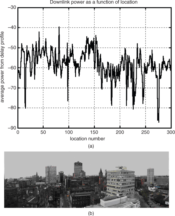
A study of location variability in Tokyo performed by Okumura gives a comparable value of 7.9 dB when calculated from the empirical relationship in the following equation [49]:
2.60 ![]()
2.11 Measurement-Based Large-Scale Path Loss Models
A number of path loss prediction models are derived from measurements such as those reported by Egli for measurements between 90 MHz and 1000 MHz [50], Young in New York at frequencies between 150 MHz and 3700 MHz [51], Allsebrook and Parsons for frequencies between 75 MHz and 450 MHz in British cities (Birmingham, Bath and Bradford) [52] and Okumura et al. at frequencies up to 1920 MHz in Tokyo [53]. Egli, Young and Allsebrook found that the median path loss value, L50, obeys the plane earth model with a correction factor β as in the following equation, which depends on the frequency and terrain:
2.61 ![]()
Expressions for β are given in Equation (2.62a) for Egli's model and Equation (2.62b) for Allsebrook and Parsons' model, where LB is diffraction loss due to buildings and γ is an additional UHF correction factor for fc >200 MHz:
where
where h0 is the average height of buildings in the neighbourhood of the mobile, hm is the mobile's height, w′ is the effective width of the street in the direction of the transmitter (the mobile is assumed to be in the middle of a street with buildings on either side) and fc is the carrier frequency (200 MHz–500 MHz).
Okumura's prediction model is the most referenced model and is derived from measurements made in Tokyo, Japan, and surrounding suburbs at 200 MHz, 453 MHz, 922 MHz, 1310 MHz, 1430 MHz and 1920 MHz. It is applied for frequencies in the range 150 MHz–2000 MHz and distances from 1 km to 100 km from the base station, base station effective antenna heights of 30 m–1000 m and receiver antenna heights typical of land mobile applications. Statistical analysis of the measurements was used to determine distance and frequency dependence of median field strength, location variability and antenna height gain factors. The basis of the Okumura model is that the path loss consists of free space loss plus an attenuation factor relative to free space, which is a function of frequency and distance. The model provides graphs that can be entered into a computer and interpolation between values can be applied to evaluate the path loss. Generally, the Okumura model is complex and gives good agreement with measurements in urban and suburban environments, but not as good in rural areas over irregular terrain. However, the urban environment defined by Okumura refers to that of Japan and does not necessarily apply to other countries.
To reduce the complexity of the Okumura method, Hata [54] established empirical mathematical relationships to describe the graphical information given by Okumura. Hata's formulation is limited to certain input parameters and is applicable only over quasi-smooth terrain. The mathematical expressions and their range of applicability are:
2.63 ![]()
2.64 ![]()
2.65 ![]()
2.66 ![]()
2.67 ![]()
When compared with the original graphs, the difference with Hata's equations is negligible and is generally less than 1 dB.
References
1. CCIR (1990) Attenuation by atmospheric gases. Doc XV11th Plenary Assembly, CCIR, Report 719-3, Vol. 5, pp. 189–204.
2. Doble, J. (1996) Introduction to Radio Propagation for Fixed and Mobile Communications, Artech House.
3. Morita, K., Inoue, T., Akeyama, A. et al. (1974) Radio propagation characteristics due to rain at 2 GHz band. Rev. Electr. Commun. Lab., (7–8), 619–632.
4. Chu, T.S. (1974) Rain-induced cross polarization at centimeter and millimeter wavelengths. Bell Syst. Tech. J., 53(8), 1557–1579.
5. ITU-R 828-2 (2006) Specific Attenuation Model for Rain for Use in Prediction Methods.
6. Davies, K. (1965) Ionospheric Radio Propagation. NBS Monograph, Vol. 80, US Department of Commerce.
7. Bertoni, H.L. (2000) Radio Propagation for Modern Wireless Systems, Prentice Hall.
8. Wilson, R. (2002) Propagation Losses through Common Building Materials: 2.4 GHz vs 5 GHz. Reflection and Transmission Losses through Common Building Materials. Report E10589, Magis Networks, Inc.
9. Huang, T.W., Lin, W.H., Lo, J.Z. et al. IEEE 802.11-09/0995r1. 60 GHz Transmission and Reflection Measurements.
10. COST Telecom Secretariat (1999) Digital Mobile Radio Towards Future Generation Systems. COST 231 Final Report, COST Telecom Secretariat, Brussels, http://www.lx.it.pt/cost231/final report.htm.
11. Green, J.A. (1992) Building penetration loss measurements for DAB signals at 211 MHz. NASA STI/Recon. Tech. Rep. N, 94, 11024.
12. Plets, D., Wout, J. and Leen, V. (2009) Extensive penetration loss measurements and models for different building types for DVB-H in the UHF band. IEEE Trans. Broadcast., 55(2), 213–222.
13. ETSI, TR (2005) ETSI, TR 102 377 v1.1.1. Digital Video Broadcasting (DVB);DVB-H Implementation Guidelines.
14. Turkmani, A. and de Toledo, A. (1993) Modelling of radio transmissions into, and within buildings at 900, 1800 and 2300 MHz. IEE Proc., 140(6), 462–470.
15. Turkmani, A. and de Toledo, A. (1991) Radio transmission at 1800 MHz into, and within multistory buildings. IEE Proc., 138(6), 577–584.
16. de Toledo, A., Turkmani, A. and Parsons, J.D. (1998) Estimating coverage of radio transmission into and within buildings at 900, 1800 and 2300 MHz. IEEE Personal Commun., 5 (2), 40–47.
17. De Yong, Y. (2001) Measurement and modeling of radiowave propagation in urban microcells. Thesis submitted to the Technische Universiteit Eindhoven–Eindhoven, Proefschrift, ISBN: 90-386-1860-3.
18. Durgin, H.X.G. and Rappaport, T.S. (1998) Measurements and models for radio path loss and penetration loss in and around homes and trees at 5.85 GHz. IEEE Trans. Commun., 46(11), 1484–1496.
19. Allen, K.C., DeMinco, N., Hoffman, J.R. et al. Building Penetration Loss Measurements at 900 MHz, 11.4 GHz, and 28.8 GHz. NTIA Report 94-306, Department of Commerce, pp. 1–106.
20. Rudd, R.F. (2003) Building penetration loss for slant paths at L-, S-, and C-band. ICAP, No 491.
21. Veltsistas, P., Kalaboukas, G. and Konotopoulos, G. (2007) Satellite to indoor building penetration loss for office environment at 11 GHz. IEEE Antennas Wireless Propag. Lett., 6, 96–99.
22. Kostanic, I., Hall, C. and McCarthy, J. (1998) Measurements of the vehicle penetration loss characteristics at 800 MHz. Proceedings of the 48th IEEE Vehicular Technology Conference, May 1998, Ottawa, ON, Canada, pp. 1–4.
23. Hill, C. and Kneisel, T. (1991) Portable radio antenna performance in the 150, 450, 800 and 900 MHz bands outside and in-vehicle. IEEE Trans. Veh. Technol., 40(4), 750–756.
24. Vogel, W.J., Torrence, G.W. and Kleiner, N. (1996) Measurement of propagation loss into cars on satellite paths at L-band. Proceedings of the 2nd European Workshop Mobile/Personal Satcoms, October 1996, Rome, Italy, pp. 129–138.
25. Tanghe, E., Joseph, W., Verloock, L. and Martens, L. (2008) Evaluation of vehicle penetration loss at wireless communication frequencies. IEEE Trans. Veh. Technol., 57(4), 2036–2041.
26. Stavrou, S. and Saunders, S.R. (2003) Factors influencing outdoor to indoor radio wave propagation. Antennas and Propagation. ICAP 2003, Conference Publication No. 491, March–April 2003, Vol. 2, pp. 581–585.
27. ITU-R 526. Propagation by Diffraction.
28. Lee, W.Y.C. (1983) Mobile Communication Engineering, McGraw-Hill Publications, New York.
29. Bullington, K. (1947) Radio propagation at frequencies above 30 Mc. Proc. IRE, 35(10), 1122–1136.
30. Epstein, J. and Peterson, D.W. (1953) An experimental study of wave propagation at 850 Mc. Proc. IRE, 41(5), 595–611.
31. Deygout, J. (1966) Multiple knife-edge diffraction of microwaves. IEEE Trans., AP14(4), 480–489.
32. Vigants, A. (1981) Microwave radio obstruction fading. Bell Syst. Tech. J., 60(8), 785–801.
33. Ament, W.S. (1953) Toward a theory of refraction by a rough surface. Proc. IRE, 41(1), 142–146.
34. Boithias, L. (1987) Radio Wave Propagation, McGraw-Hill Inc., New York.
35. Bacon, D.F. (1996) Introduction to Diffraction, Reflection and Scattering, in Propagation of Radio Waves (eds M.P.M. Hall, L.W. Barclay and M.T. Hewitt), The Institution of Electrical Engineers.
36. Skolink, I.M. (2001) Introduction to Radar Systems, McGraw-Hill Inc., Boston, MA.
37. Xia, H.H., Bertoni, L.H. and Maciel, R.L. (1993) Radio propagation characteristics for line of sight microcellular and personal communications. IEEE Trans. Antennas Propag., 41(10), 1439–1446.
38. Loyka, S., Kouki, A. and Gagnon, F. (2001) Fade depth prediction on wireless microwave links using two ray multipath model. 2001 Canadian Conference on Electrical and Computer Engineering (CCECE 2001), 13–16 May 2001, Toronto, ON, Canada.
39. Jordan, E.C. and Balmain, K.G. (1968) Electromagnetic Waves and Radiating Systems, Prentice Hall, New York.
40. Salous, S. (1989) Measurement of narrow pulse distortion over a short HF skywave link Es and F2 summer results. Radio Sci., 24, 585–597.
41. Epstein, M.R. (1969) Polarization of ionospherically propagated hf waves with application to radio communication. Radio Sci., 4, 53–67.
42. Salous, S. and Gokalp, H. (2002) Dual frequency division duplex sounder for UMTS frequency division duplex channels. IEE Proc. Commun., 149(2), 117–122.
43. Salous, S. and Hinostroza, V. (2005) Wideband indoor frequency agile channel sounder and measurements. IEE Proc. Microwaves Antennas Propag., 152(6), 573–580.
44. Jakes, W.C.Y. (ed) (1947) Microwave Mobile Communications, John Wiley & Sons, Inc., New York.
45. Salous, S., Feeney, S., Khokhar, K. and Lewemz, R. (2008) Measurements of radio channels and bit error rate estimation of IEEE802.16 standard in semi-rural environment at three frequencies in the 2–6 GHz frequency band average fade bandwidth. IET Commun., 2(7), 878–885.
46. Salous, S. and Gokalp, H. (2007) Medium- and large-scale characterization of UMTS-allocated frequency division duplex channels. IEEE Trans. Veh. Technol., 56(5), 2831–2843.
47. Ibrahim, M.F. and Parsons, J.D. (1983) Signal strength prediction in built-up areas. Part I: median signal strength. Proc. IEE, Pt. F, 130(5), 377–384.
48. Salous, S. and Gokalp, H. (2001) Estimation of location variability from wideband channel sounding measurements. COST 273 TD(01) 029, 15–17 October 2001, Bologna, Italy, pp. 1–6.
49. Saunders, S. (2000) Antennas and Propagation for Wireless Communication Systems, John Wiley & Sons, Ltd.
50. Egli, J. (1957) Radio propagation above 40 Mc over irregular terrain. Proc. IRE, 45, 1383–1391.
51. Young Jr, W.R. (1952) Comparison of mobile radio transmission at 150, 450, 900, and 3700 Mc. Bell Syst. Tech. J., 31, 1068–1085.
52. Allsebrook, K. and Parsons, J.D. (1977) Mobile radio propagation in British cities at frequencies in the VHF and UHF bands. IEEE Trans. Veh. Technol., VT-26, 313–322.
53. Okumura, Y., Ohmori, E., Kawano, T. and Fukuda, K. (1968) Field strength and its variability in VHF and UHF land mobile radio service. Rev. Electr. Commun. Lab., 16(9–10), 825–873.
54. Hata, M. (1980) Empirical formula for propagation loss in mobile radio services. IEEE Trans. Veh. Technol., VT-29, 317–325.