Chapter 3
Radio Channel Models
Radio channel models for narrowband and wideband transmissions are commonly used to predict coverage of a wireless link and system performance. These are classified as (i) deterministic models, (ii) statistical/empirical models and (iii) semi-deterministic or site specific models. Ray tracing models are deterministic in that the received signal can be computed from knowledge of the geometry of propagation, the electrical properties of the medium of propagation, radar cross section of objects and antenna radiation pattern. A ray tracing algorithm aims to determine all the contributing propagation mechanisms at the receiver location such as free space if a line of sight (LOS) component is present, all the reflected and refracted components, all the diffracted components and all the scattered components. The technique is computationally inefficient for large urban environments and is more suited to small areas such as indoor environments or propagation over small sections of a street. Statistical models are measurement based and thus are dependent on the measurement equipment, the experimental set-up and the environment. Corrections for some of the parameters such as antenna height above ground or frequency are sometimes generated to account for differences between the measured data in the model and the scenario in which the model is to be applied. Such an example is the Okumura model where correction curves have been generated [1]. Semi-deterministic or site specific models use ray tracing to identify the main rays in a specific site and superimpose statistical distributions.
A widely adopted model is based on systems theory where the parameters of the model can be deterministic or statistical. In this chapter the systems channel models are discussed for both narrowband and wideband channels. In a multipath environment narrowband refers to a flat fading channel where all the frequency components in the signal have similar amplitude variations, whereas a wideband channel suffers from frequency selectivity. In a frequency dispersive channel, distortion of narrow pulses and frequency modulated continuous wave (FMCW) or chirp pulses due to phase nonlinearity are outlined to illustrate the effects of deviation from ideal transmission conditions. The various models are first analyzed for time-invariant conditions followed by time-variant environments. Small-scale channel parameters experienced over a few wavelengths or over a short time interval are defined for single input–single output (SISO) systems. Finally, various stochastic and physical channel models that determine the capacity of multiple input–multiple output (MIMO) systems are outlined.
3.1 System Model for Ideal Channel: Linear Time-Invariant (LTI) Model
Ideal transmission of a signal through any medium assumes that the signal does not suffer from any form of distortion and remains unchanged with time; that is it is time invariant. Thus the only two acceptable modifications of the signal z(t) as it passes through the medium of transmission are a delay in the time of arrival and a change in the overall magnitude, which can be due to a constant attenuation or magnification factor. Under these conditions, the received signal y(t) is expressed as:
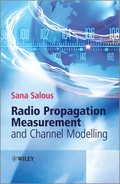
where z(t) is the transmitted signal, A is a constant and τ is the delay due to the propagation time through the medium. In the more generalized case, a time-invariant radio channel can be considered as a linear filter characterized by its response h(t) due to an impulse δ(t) at its input or its frequency response H(ω), as shown in Figure 3.1. Time invariance implies that the impulse response is independent of the time of applying the excitation such that δ(t − τ) gives h(t − τ).
Figure 3.1 Time-invariant system model of radio channel: (a) time domain and (b) frequency domain.
Taking the Fourier transform (FT) of Equation (3.1) and the ratio of the output to the input gives the ideal frequency response of the channel as:
The corresponding ideal impulse response is given by:
The output z(t) is then found from the convolution integral for continuous time signals or from the convolution sum for the discrete time domain:
3.4 
Any deviation from the conditions in Equation (3.3) in either amplitude or time delay results in signal distortion and requires compensation in the design of communication systems. Since radio signals are bandpass signals, it is usual to express the input and output in terms of their lowpass (LP) complex envelope representation; that is,
3.5 
where z(t) and y(t) are bandpass signals and y0(t) and z0(t) are the complex envelope of the LP signals.
Under this representation the LP impulse response, ho(t) of the channel becomes:
Equations (3.3) and (3.6) imply that the response of the radio channel due to an impulse at the input should be an impulse that can be amplitude scaled and time delayed and Equation (3.2) states that the system's frequency response should be flat over the entire frequency range with a linear phase function. Deviations from either constant amplitude due to, for example, frequency selectivity that results from multipath propagation or deviation from linear phase due to frequency dispersion gives rise to distortion and hence nonideal propagation conditions. Figure 3.2 gives the ideal channel model in both the time domain and in the frequency domain. In the time domain this consists of a multiplier and a time delay block, whereas in the frequency domain this consists of a multiplier and a phase shifter.
Figure 3.2 Ideal channel model: (a) in the time domain and (b) in the frequency domain.
3.2 Narrowband Single Input–Single Output Channels
A narrowband signal can be modelled by a single CW transmission. In the following we will consider narrowband transmission first assuming a single propagation path and then the more generalized scattering model.
3.2.1 Single-Path Model
Considering first distortionless transmission, Equation (3.2) becomes equal to:
3.7 ![]()
This means that the amplitude of the sinusoid is modified by a constant multiplying factor A, while its phase is shifted by a constant value equal to ![]() . From a system's perspective this means that the channel function is time invariant and single valued at that particular frequency.
. From a system's perspective this means that the channel function is time invariant and single valued at that particular frequency.
Assume now that the time delay of propagation varies with time due to changes in the phase path length p(t), but the amplitude remains constant. Then as in Equation (1.128) the received signal can be expressed with the time delay variations being rewritten as a phase shift:
3.8 ![]()
Taking the time derivative of the phase, the instantaneous frequency fi of the received signal can be written in terms of the Doppler shift fD as:
3.9 ![]()
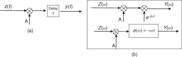
If the phase shift varies in a random manner with time, the effect is to have a frequency modulated carrier, referred to as random frequency modulation. Since the amplitude of the received signal can also vary with time the generalized single-path system's model for a single frequency component is as shown in Figure 3.3.
Figure 3.3 Single-path propagation model for narrowband transmission.
In general, in a multipath environment the received signal consists of a large number of replicas of the transmitted signal, each with its own amplitude coefficient and Doppler shift, as discussed next in the scattering model.
3.2.2 Multipath Scattering Model
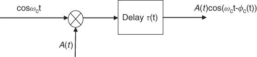
In mobile radio studies it is customary to model the phase variation by a Doppler spectrum with a U shape. This is based on the scattering model, which assumes a large number of multipath components. The actual shape depends on the assumptions with regard to the multipath structure and the angle of arrival of the multipath components in azimuth and in elevation. Referring to Figure 3.4a and b it is seen that the received signal can travel via several possible paths with different angles of departure from the transmit antenna and arrive with different angles at the receive antenna.
Figure 3.4 Multipath propagation: (a) indoor environment, (b) outdoor environment and (c) angle of arrival of a single wave.
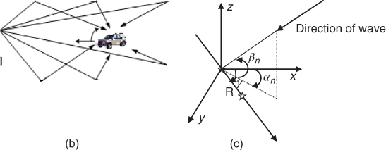
To derive the scattering model, consider first a vertically polarized wave arriving at a point in space with angle αn with the horizontal plane and an angle βn in elevation as in Figure 3.4c. The received electric field due to the nth multipath component is given by:
where aR is the unit vector along R, β is the wave number, aβ is the unit vector along the direction of wave propagation and · is the dot product between the two unit vectors.
Expanding the vectors along the xyz axes gives the following relationships:
3.11a ![]()
3.11b ![]()
Taking the dot product in Equation (3.10) and taking the real part, the received electric field can be expressed as:
3.12 ![]()
where Φn is a phase shift with respect to an arbitrary reference.
When the mobile moves with velocity ν in the xy plane in a direction making an angle γ to the x axis, in a time interval Δt the new xyz coordinates are:
The electric field at the new point is then expressed as:
3.13 
The term ![]() gives a time-varying component. Taking its derivative with respect to time gives an angular frequency offset equal to:
gives a time-varying component. Taking its derivative with respect to time gives an angular frequency offset equal to:
3.14 ![]()
This frequency shift from the carrier is the Doppler shift of the nth multipath component.
Assuming for simplicity that (xo, yo, zo) are at the origin then the received electric field is:
3.15 ![]()
In general a large number of components are received and each component will experience a different attenuation factor and a different Doppler shift. Hence, the overall received electric field E(t) is given by:
where I(t) and Q(t) are called the in-phase and quadrature components.
Due to the random nature of mobile radio propagation, a number of assumptions are usually made with regard to the angle of arrival, phase shift and amplitude of the received electric field. Three models have been proposed to accommodate these parameters. The first model was proposed by Clarke [2] in an attempt to explain the statistical characteristics of the received signal by a mobile vehicle in an urban environment. This model was later modified by Aulin [3] and subsequently by Parsons [4].
Common to all the three models are the following assumptions:
3.17 ![]()
In his model Clarke assumed that the waves have identical amplitude, Eo, whereas in Aulin's model the amplitude of the received waves was assumed to be a random variable independent of the other random variables in Assumption 1 with a variance given by:
3.18 ![]()
where Eo is a constant and E stands for the expected value.
Since in an urban environment a large number of waves are likely to arrive at the antenna of the mobile vehicle, by the central limit theorem, which can be satisfied for N ≥ 6 [5], the quadrature components I(t) and Q(t) are independent Gaussian processes with zero mean and variance σ2, where the Gaussian probability density function (PDF) is given by:
3.19 ![]()
The resultant envelope r(t) and phase θ(t) of the received signal are then given in terms of the quadrature components as in:
3.20a ![]()
3.20b ![]()
and the envelope has a Rayleigh distribution as given by [6]:
3.21 ![]()
Due to the random nature of the received signal, to evaluate the Doppler spread we need the autocorrelation function of Equation (3.16), which is given by the expected value of E(t) with a time-shifted version as in:
where a(τ) and c(τ) are given by:
![]()
Taking the FT of Equation (3.22) gives the power spectral density of the received signal. The shape of this spectrum is related to the distribution of the elevation angle as assumed in each of the three models discussed below.
3.2.2.1 Clark's Model
Clarke [2] proposed a two-dimensional model where the waves are assumed to arrive in the horizontal plane only, thus ignoring the elevation angle βn, which is represented as an impulse:
3.23 ![]()
Based on this assumption, Clarke showed that:
where J0 is the zero-order Bessel function of the first kind and the maximum Doppler shift, fm = v/λ and c(τ) = 0.
Taking the FT of Equation (3.24), the power spectrum of the received baseband signal is given by:
3.25 
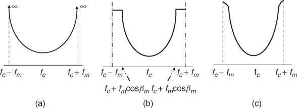
The spectrum in Equation (3.24) is strictly band-limited within the maximum Doppler shift (fm = v/λ), but the power spectral density becomes infinite at fc ± fm, as illustrated in Figure 3.5a.
Figure 3.5 Doppler spectra of received signal using different parameters for the scattering model: (a) Clarke's model, (b) Aulin's model and (c) Parsons' model.
3.2.2.2 Aulin's Model
Aulin [3] proposed a three-dimensional model since he postulated that the angles of arrival cannot all fall in the horizontal plane. Thus he proposed the following PDF for β:
Using the PDF in Equation (3.26), Aulin showed that:
3.27 
which has a FT given by:
The spectrum in Equation (3.28) is sketched in Figure 3.5b and is seen to have a constant value for ![]() , which is unrealistic and does not correspond to what is observed from mobile radio measurements.
, which is unrealistic and does not correspond to what is observed from mobile radio measurements.
3.2.2.3 Parsons' Model
To avoid the discontinuity at the edge in Clarke's model and the constant value of Aulin's model, Parsons [4] proposed a different PDF for β, which has a mean value of 0° and is heavily biased towards small angles given by:
3.29 
The power spectrum is then evaluated using numerical techniques. As can be seen from Figure 3.5c, the spectrum goes smoothly towards the maximum value and avoids the discontinuity at the edge.
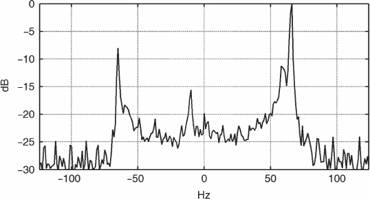
All the above spectra have been derived for a narrowband signal and show the spread of the power of the received signal around the carrier. An example of a Doppler spectrum obtained from measurements at 2 GHz over a 1 second time interval is shown in Figure 3.6. While it resembles the theoretical curves in Figure 3.5, it is not entirely symmetric as the theoretical spectrum. To obtain the theoretical U-shaped model it is necessary to satisfy the assumptions of the model. Averaging over a long period of time, the measured spectrum might eventually converge to the U-shaped spectrum. The U-shaped spectrum is commonly referred to as the Jakes spectrum.
Figure 3.6 Doppler spectrum from measured data where the carrier is set at 0 Hz.
3.3 Wideband Single Input–Single Output Channels
In Section 2.8 we discussed the effects of multipath on a radio signal as a function of time, space and frequency. Frequency dispersion due to variations in the group time delay has also been presented in Section 1.8 in relation to propagation via the ionosphere. This section discusses the effects of both multipath distortion and frequency dispersion on digital data transmission.
3.3.1 Single-Path Time-Invariant Frequency Dispersive Channel Model
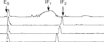
To study the effects of phase nonlinearity we will consider here HF propagation via the ionosphere where different frequencies travel over different path lengths that result in a nonlinear phase function of the channel and distort the received signal. Distortion effects of narrow pulses using the phase function in Equation (1.127) have been studied in [7–11] and for chirp pulses which are FMCW signals in [12, 13]. They all concluded that the effect of phase nonlinearity on the transmission of a narrow pulse or a chirp pulse can be related to the derivative of the group time delay as a function of frequency. They also concluded that the effect of phase nonlinearity is to elongate the pulse duration in time and to distort its amplitude, as illustrated in Figure 3.7 for an 8 µs pulse propagating via different layers of the ionosphere. The shape and width of the pulse is seen to vary depending on the reflecting layer, with the pulse transmitted via the 1F1 layer suffering the most broadening as it goes through the highest slope of group time delay versus frequency when the maximum usable frequency is reached.
Figure 3.7 Pulse distortion due to phase nonlinearity over an ionospheric channel.
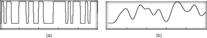
This broadening of the pulse limits the data rate of a digital communication system since a pulse transmitted prior to the decay of the response of the first received pulse will result in interference between the two pulses and it would not be possible to distinguish them without coding and equalization. This effect is known as intersymbol interference (ISI) and is illustrated in Figure 3.8. To maximize the data rate it is therefore desirable to transmit with a pulse width commensurate with the narrowest pulse width that can be achieved via a particular channel.
Figure 3.8 Transmission of digital data through a dispersive medium where the bit duration is shorter than the impulse response: (a) original data stream and (b) received data stream.
The analysis to estimate pulse broadening and the optimum bandwidth of transmission is based on the channel frequency response model given as:
In Equation (3.30) the phase function is based on Equation (1.127), as given by:
where
![]()
and τg is the group time delay of the channel as a function of frequency. The quadratic frequency term in Equation (3.31) gives the phase nonlinearity of the channel.
Two models for the channel amplitude function have been used in the analysis. One model assumes constant amplitude versus frequency [8] as in Equation (3.32a) and the second model assumes a Gaussian shape function [11, 13] as in Equation (3.32b):
The envelope of the frequency response gives a parabolic curve of attenuation in decibels plotted against frequency, with a minimum attenuation at ωc and a 6 dB bandwidth Bch:
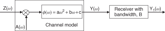
Due to the finite bandwidth of the receiver, it is necessary to include the receiver in the analysis as shown in Figure 3.9, which represents a single multipath component. For a radio channel with a number of multipath components, each component has its frequency response represented by an envelope function and quadratic phase function as in Equations (3.32a), (3.32b) and 3.33.
Figure 3.9 Single-path time-invariant frequency dispersive channel model used in analysis of narrow pulse transmission.
3.3.1.1 Narrow Pulse Distortion
Taking the inverse Fourier transform (IFT) of Y1(ω) and using the same phase function in Equation (3.31), Sollfrey [8] and Inston [11] obtained mathematical expressions for the width of the received pulse. Under the assumptions of Equation (3.32a) for the amplitude function Sollfrey [8] solved the following equation to evaluate the distortion of narrow pulses:
The solution to Equation (3.34) was evaluated in the form of a Fresnel integral, which had to be solved numerically. Similarly, Inston [11] solved the following equation to estimate pulse distortion:
Both Sollfrey [8] and Inston [11] relate the length of the received pulse to the slope of the group time delay and the 6 dB width of the channel. Figure 3.10 displays narrow pulse distortion as estimated by Sollfrey [8], where in the figure α refers to the ratio of the receiver bandwidth and B to the channel bandwidth, defined as:

Figure 3.10 Pulse distortion due to phase nonlinearity as estimated by Sollfrey [8]. Source: Sollfrey, W., (1965) Effects of propagation on the high frequency electromagnetic radiation from low altitude nuclear explosions, Proc. IEEE, 53, 2035–2042.
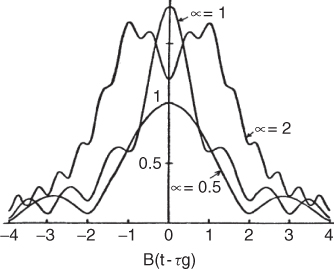
Thus the channel bandwidth is determined by the slope of the group time delay of the channel. Figure 3.10 shows that when the receiver bandwidth matches the channel bandwidth as determined by phase nonlinearity, the width of the received pulse is optimum. When the bandwidth of the receiver is wider than the channel bandwidth α = 2, then the pulse is distorted due to phase nonlinearity whereas when the receiver bandwidth is smaller than the channel bandwidth α = 0.5, the dispersion of the pulse results from limiting the bandwidth of the signal. The expression for the optimum narrow pulse width to be transmitted via a channel with a nonlinear phase function as derived by Sollfrey [8] is:
3.36 ![]()
Evaluating the integral in Equation (3.35) and solving for 1/e down from the peak, Inston [11] arrived at the following expression for the width of the dispersed pulse:
Plotting Equation (3.37) with ![]() versus
versus ![]() Inston [11] deduced that the channel exhibits three modes of behaviour, as summarized by:
Inston [11] deduced that the channel exhibits three modes of behaviour, as summarized by:
3.38a ![]()
3.38b ![]()
In the narrowband case variations of the group time delay across the bandwidth are negligible and thus the pulse length is inversely proportional to the channel bandwidth. In the broadband behaviour, the pulse length is related to the difference in group arrival times of the limit frequencies of the bandwidth. Minimum pulse distortion as in Equation (3.38c) occurs between these two limits.
3.3.1.2 Chirp Pulse Distortion
A chirp signal is characterized by a linear frequency increase or decrease over a bandwidth B, in a time interval equal to T. It is characterized by its sweep rate, χ = π(B/T) and its time bandwidth product BT, which determines the shape of its spectrum. At the receiver the chirp signal is compressed in time duration from a pulse of duration equal to T to a pulse that has a 4 dB width equal to 1/B. This time compression can be affected by phase nonlinearity, which can elongate the pulse similar to the narrow pulse case.
In [13] distortion of chirp pulses by the ionosphere was estimated by substituting the spectrum of the chirp signal given by:
3.39 ![]()
into Equation (3.35) and solving:
The solution for Equation (3.40), which represents the received signal prior to detection by the receiver, is given by:

where ![]() ,
, ![]() ,
, ![]() ,
, ![]() and
and ![]() .
.
Detection of chirp pulses is achieved using either a matched filter or a correlation detector. In the latter the output of the detector is a signal that is compressed in bandwidth but not in time (see Section 4.12 for a detailed analysis of chirp signals). Time compression is subsequently achieved via spectrum analysis, where each multipath component is represented by a low frequency component. Passing the signal in Equation (3.41) through the correlation detector, in [13] the effective input into the spectrum analyzer is shown to be a frequency modulated signal with a Gaussian envelope. The instantaneous frequency of the pulse fi and its 6 dB width T2 (for ![]() ) are given by:
) are given by:
3.42b 
Equation (3.42a) is similar to Equation (3.37) where the sweep rate B/T replaces the time derivative of the group time delay. Thus plotting ![]() versus
versus ![]() produces three regions, that is narrowband, wideband and optimum or minimum width. These are obtained as:
produces three regions, that is narrowband, wideband and optimum or minimum width. These are obtained as:
3.43a ![]()
3.43b ![]()
3.43c ![]()
Since the output of the detector is a frequency modulated signal instead of the ideal sinusoid, to evaluate its compressed width following spectral analysis it is necessary to find the total frequency deviation of the pulse ΔF and its time bandwidth product. The frequency deviation ΔF is first found from the time derivative of the instantaneous frequency and the width of the pulse as:
where
and
![]()
where ![]() is the floor function. The corresponding time bandwidth product|ΔF|T3 is given by:
is the floor function. The corresponding time bandwidth product|ΔF|T3 is given by:

The first term in Equation (3.44) is a function of the derivative of the group time delay or phase dispersion whereas the second term is a function of the bandwidth of the channel. To identify the two terms they are referred to as ‘phase dispersion’ and ‘amplitude dispersion’ respectively. The result in Equation (3.45) shows four regions where Equation (3.45a and b) can be considered as the wideband case and Equation (3.45c and d) as the narrowband case. Consider the wideband case; the ‘phase dispersion’ term in Equation (3.44) is equal to ![]() and an optimum transmission bandwidth that results in a compressed spectrum width equal to 1/T occurs when:
and an optimum transmission bandwidth that results in a compressed spectrum width equal to 1/T occurs when:
3.46 
This condition means that the bandwidth of the transmitted chirp signal should match the bandwidth of the channel both in amplitude and in phase delay.
In the narrowband case, amplitude dispersion dominates and the time bandwidth product of the dispersed signal (Equation (3.45c and d) is significant and in particular Equation (3.45d) indicates that no compression of the received signal has been achieved. For these cases the optimum bandwidth of transmission as determined by ‘amplitude dispersion’ is equal to 1.136Bch for Equation (3.45c) and 1/T for Equation (3.45d).
3.3.2 Single-Path Time-Variant Frequency Dispersive Channel
For a time-variant channel, the amplitude, phase time delay and group time delay of the channel vary with time. The resulting time-variant transfer channel model is then given by:
where a second order Taylor series expansion is used to express the phase function:

Equations (3.47a) and (3.47b) can be written in a more compact form by letting:

where
The expression in the first parentheses in Equation (3.48) is the time-invariant model given by:
3.49 ![]()
The expression in the second parentheses in Equation (3.48) contains all the time-variant parameters and thus its derivative gives the time-variant Doppler shift as:
3.50 ![]()
For each propagation path the received channel model is shown in Figure 3.11.
Figure 3.11 Nonlinear time-variant phase channel model.
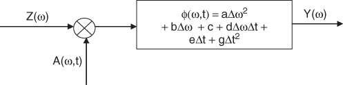
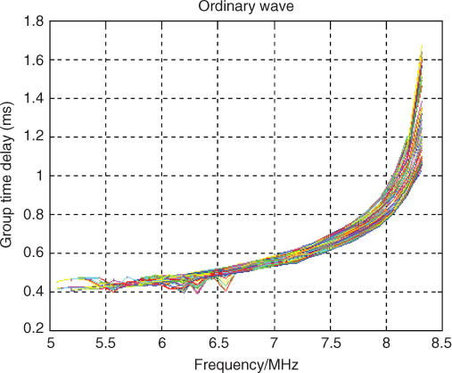
Figure 3.12 shows an example of the time and frequency variations of the group time delay of the ordinary wave over 900 seconds from data acquired every 10 seconds over a short skywave radio link in the UK [13]. Taking the derivatives from these curves and the group time delay, the coefficients a to d in Equation (3.48) can be evaluated. The rest of the coefficients pertaining to the Doppler shift and its time derivative require phase coherent measurements of the phase variations versus time.
Figure 3.12 Group time delay variations as a function of frequency and time.
3.3.3 Multipath Model in a Nonfrequency Dispersive Time-Invariant Channel
Multipath propagation extends the duration of the received pulse as illustrated in Figure 3.13. For a time-invariant channel the multipath structure does not vary with time either in amplitude or in time delay.
Figure 3.13 Channel impulse response due to multipath propagation.
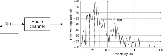
Hence, the effect of multipath on data transmission is similar to phase nonlinearity and gives rise to ISI for high data rates when symbols are transmitted prior to the decay of the impulse response. By sampling the impulse response at equal time intervals separated by Δt as shown in Figure 3.13 and fixing the amplitude during each time interval, the impulse response of the channel h(t) becomes the sum of weighted and delayed impulses, as given by Equation (3.51a), while the corresponding discrete time domain representation is given by Equation (3.51b):
Taking the FT gives the corresponding frequency response as:
3.52 
3.3.3.1 Time Domain Model
Implementation of the impulse response in Equations (3.51a) and (3.51b) represents the time domain model of the channel in what is commonly known as the tapped delay line shown in Figure 3.14.
Figure 3.14 Tapped delay line implementation of the time-invariant finite impulse response.
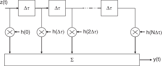
The tapped delay line model assumes a finite duration impulse response, which is a reasonable assumption for all radio channels, and hence the sum in Equations (3.51a) and (3.51b) has a maximum limit equal to N as in:
Using the low-pass (LP) complex representation, the coefficients in Equation (3.53) would have complex values.
The tapped delay line implementation requires a number of taps related to the length of the impulse response of the channel and the time delay separation between the taps as in Figure 3.13. The value of Δt is related to the time delay resolution, which is inversely proportional to the bandwidth of the system. For example, for a 10 MHz signal transmitted over a channel with a maximum time delay τmax of 1 µs, the separation between taps is 100 ns and the total number of taps is 10. The tapped delay line model has generally been popular due to its simplicity and the limited number of multipath components.
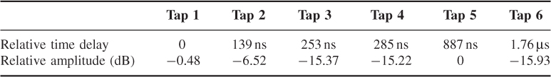
Figure 3.15 displays the multipath structure obtained with a 16.6 ns time pulse and the corresponding frequency domain representation H(ω). Inspecting the multipath structure, although a number of multipath components are present, there are two dominant paths of comparable magnitude with ∼0.9 µs time delay difference. Using the approximate equation for the two-ray model, this gives a frequency separation between minima as 1.1 MHz, which is consistent with the frequency domain representation. Hence, for this example components that are significantly (∼18–20 dB) below the main component(s) can be discarded, resulting in a fewer number of taps. For many applications three to four taps are used in the model where each tap is defined in terms of its relative time delay with respect to the first component and the relative amplitude. For the example in Figure 3.15, six taps can be specified for an 18 dB threshold, as given in Table 3.1.
Figure 3.15 Time domain response obtained at 2 GHz with 16.67 ns time delay resolution and the corresponding frequency response.
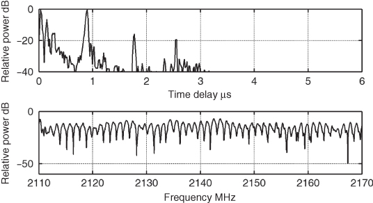
Table 3.1 Relative time delay and relative amplitude for the main taps of Figure 3.14
3.3.3.2 Frequency Domain Model
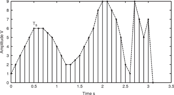
To obtain the frequency domain model, the counterpart of the time domain sampling theorem needs to be implemented. In time domain sampling, a band-limited signal x(t) with bandwidth equal to ωm has to be sampled at least at 2ωm. The sampled signal is then reconstructed by interpolating between the samples using the ideal sinc function as given in the following equation, where Ts is the time separation between samples, as displayed in Figure 3.16:
3.54 ![]()
Figure 3.16 Sampling of continuous time signal.
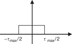
Similarly, a time-limited signal that extends between −τmax/2 and τmax/2 as in Figure 3.17 can be constructed from its frequency domain samples using the sinc interpolating function if the samples are at least at 1/τmax seconds. Thus a channel with a finite impulse response h(t) can be represented by its sampled frequency response, as given by:
3.55 ![]()
Figure 3.17 Time domain signal limits.
This implies that the incoming signal would have to be filtered into narrowband sections, which are then multiplied by the frequency response of the channel at the centre frequencies of the subbands and added together as shown in Figure 3.18. The frequency function of the filters in the frequency response is derived on the basis that the channel time delays are restricted between 0 and the maximum time delay τmax which is centred at τ0. This gives a subband filter function as in Equation (3.56) and a corresponding impulse response as given in Equation (3.57) [14]:
Figure 3.18 Frequency domain channel function illustrating the frequency slices.
Source: Khawar Khokhar, (2006) Design and development of mobile channel simulators using digital signal processing technqiues, Durham Theses, Durham University. Available at Durham E-Theses Online: http://etheses.dur.ac.uk/2948/. Reproduced with permission.
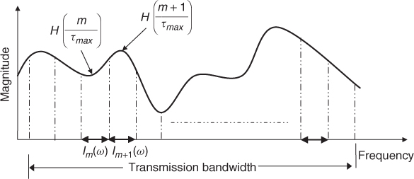
Considering the two-ray model, the frequency domain representation would require at least two samples per cycle, which corresponds to filters separated by at least 2/τmax. In general, many more filters are required and Bello suggested that the number of sections used is equal to 10Bτmax, where B is the bandwidth of the signal [14] and in [15] the required number of branches was found to be 10πBτmax. Therefore, for the same example of the tapped delay line model, for a signal with 10 MHz bandwidth and τmax equal to 1 µs, the number of sections is equal to 100–314 in contrast to the 10 taps required for the time domain tapped delay line model. This high requirement for a large number of sections in the frequency domain makes the time domain tapped delay line more popular.
3.3.4 Multipath Propagation in a Nonfrequency Dispersive Time-Variant Channel
3.3.4.1 Time Domain and Frequency Domain Models
For a time-variant channel, if an input δ(t) gives rise to h(t), then delaying the input by τ to δ(t − τ) gives a response hτ(t) that is different from h(t). To account for the time variability of the channel response Zadeh [16] introduced the time-variant impulse response h(t,τ), which gives the convolution relationship:

For such a system, the frequency domain representation is obtained by taking the FT of Equation (3.58) with respect to the time delay variable τ. This gives the frequency response of the channel, which is also time variant. In general, if z(t) forms the input to the channel, the output signal is obtained from the IFT, as given by:
3.59 
where
Figure 3.19 gives the time and frequency domain time-variant system functions.
Figure 3.19 Time-variant system functions: (a) time domain function and (b) frequency domain function.
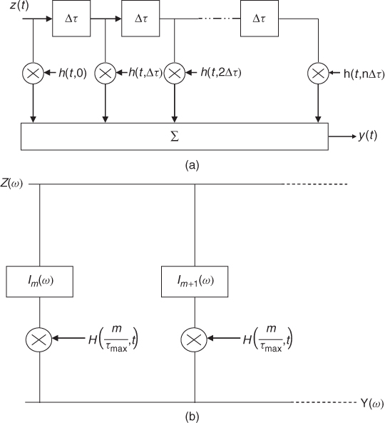
The convolution in Equation (3.58) can be implemented by a tapped delay line similar to that in Figure 3.14 where now the coefficients are time variant as given in Equation (3.60a). The tapped delay line aids in realizing the system functions either in a hardware digital implementation or a software simulator and the resultant model is shown in Figure 3.20a. Alternatively, the output can be estimated from the time-variant frequency function as in Equation (3.60b) (see also Section 6.3.2) and as illustrated in Figure 3.20b:

Figure 3.20 (a) Tapped delay line implementation of the time-variant channel function and (b) frequency domain implementation of the time-variant frequency response.
3.3.4.2 Other Channel Functions
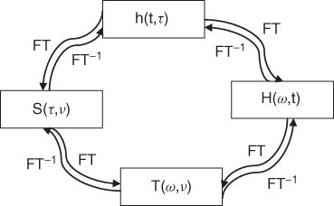
Two other channel functions that are also related by a FT to the time-variant impulse response and the time-variant frequency response are the delay Doppler function obtained by taking the FT of h(t,τ) and the frequency Doppler function obtained by taking the FT of H(ω,t), both with respect to the time variable t. These give the respective functions S(τ,ν) and T(ω,ν):


where ν is a frequency variable and represents the Doppler shift in radians/seconds. Figure 3.21 displays the FT relationship between the different functions.
Figure 3.21 System function representation of the radio channel.
Using Equation (3.61) the output can be found from the following relationships:
3.62 
3.3.5 Multipath Propagation in a Frequency Dispersive Time-Variant Channel
The generalized channel model is obtained when time variations occur in the presence of multipath propagation as well as phase nonlinearity. In this case, the frequency response of the channel can be written as:
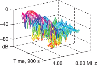
where the phase function for each multipath component is expressed as in Equation (3.48). In Equation (3.63) each multipath component can have a frequency function that is both frequency and time dependent, as in the case of ionospheric propagation. An example of amplitude variations with time and frequency of the ordinary wave is shown in Figure 3.22 over 900 seconds across a frequency range of 4.88–8.88 MHz.
Figure 3.22 Amplitude of the frequency time function of an ordinary wave.
3.4 System Functions in a Linear Randomly Time-Variant Channel
In a mobile radio environment as the user moves between streets and terrains, the variations in the environment cause variations in the multipath structure. Similarly, as the sun intensity varies with the time of day and time of year, the electron density in the ionosphere varies with time, giving rise to a different multipath structure. Generally, due to the large number of multipath components and the random motion of the user or the propagation medium, the resultant signal variations can be characterized via stochastic distributions rather than a deterministic model.
For the example of the time domain tapped delay line model, due to the high number of multipath components it is assumed that each coefficient of the channel taps also consists of a large number of components and hence is represented by a PDF. Different PDF models exist to study the statistical behaviour of each tap. Due to the nature of the time or spatial variations, these are normally divided into three types of variations. Small-scale variations occur over short time intervals or short spatial distances (usually a few wavelengths) and are characterized by fast random variations. Medium-scale variations occur over a few hundred metres or hourly time intervals as in the ionosphere. Large-scale variations occur when the user moves over large distances, possibly several kilometers, or long time intervals, such as the 11 year sunspot cycle. To obtain full statistical characterization, both small-scale and medium- or large-scale variations need to be modelled for a complete representation of the time-varying channel behaviour.
The choice of small-scale PDFs depends on whether a dominant component such as a direct LOS component is present or not, the environment surrounding the user antenna and the distance to the scatterers/reflectors. The widely employed statistical distributions are Rayleigh, Rician, Nakagami, Weibull, log-normal and Suzuki [17–20]. Large-scale variations are generally modelled by a log-normal distribution. Appendix 1 gives the various PDFs of the distributions and their properties.
In principle each tap in the time domain tapped delay line can be modelled by a different distribution. The Rayleigh distribution is used in the absence of a dominant component where a large number of independent components with equal amplitude have been received (≥6), each with a random phase and with uniform distribution in the range (0–2π) [21–23]. The Rician distribution is used when a dominant component is received in addition to a large number of scattered components where the power of the dominant component is greater than the sum of the power of all the other components; this ratio is denoted as the K factor, which reduces to a Rayleigh distribution when the K factor goes to zero. Unlike the Rayleigh and Rician distributions the Nakagami model provides the possibility of different amplitudes for the scattered waves and partial correlation between the scattering elements. It usually models channel conditions that are either more or less severe than the Rayleigh distribution [20, 24, 25]. The log-normal distribution is applicable where the propagation environment has tall buildings and trees that give rise to multiple reflections or multiple scattering, which introduces further fluctuation in the received signal [26–29]. Suzuki's model [26] incorporates both small-scale and large-scale variations in a single distribution, where the short term variations are modelled as Rayleigh and the long term variations as log-normal.
The system functions in Figure 3.21 now become stochastic processes that in principle require knowledge of all the joint PDFs of the process, which is difficult to achieve. To overcome this difficulty Bello [14] suggested using the following autocorrelation functions:
3.64c ![]()
3.64d ![]()
where t and t′ are time variables, τ and τ′ are time delay variables, ω and ω′ are frequency variables and ν and ν′ are Doppler shift variables; * indicates the complex conjugate and E is the expected value of the ensemble of the process.
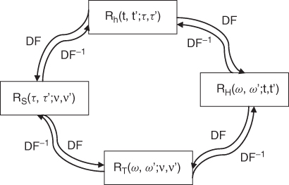
Similar to the Bello system functions presented in Figure 3.21, the system autocorrelation functions are also related by the FT, where now due to the correlation function they are interrelated by the double Fourier transform and its inverse function, denoted by DF and IDF, respectively. Figure 3.23 gives the relationships between the system autocorrelation functions.
Figure 3.23 Relationship between different autocorrelation functions.
3.5 Simplified Channel Functions
Two types of simplified channel models are commonly used, namely the wide-sense stationary (WSS) channel and the uncorrelated scattering (US) channel.
3.5.1 The Wide-Sense Stationary (WSS) Channel
Over short periods of time or over small spatial distances, mobile radio channels are assumed to be stationary in the wide sense or weakly stationary. WSS channels have the property that the channel correlation functions are invariant under a translation in time or space. This means that the fading statistics do not change over a short time interval and the autocorrelation function is independent of the absolute time; that is it is only a function of the time difference Δt = t − t′. Hence the time dependent correlation functions in Equations (3.64a) and (3.64b) reduce to:
3.65a ![]()
3.65b ![]()
Taking the double Fourier transform of Equation (3.64a) with respect to the time variable, and using the conjugate of the complex exponential in the transform, gives:

The first integral in Equation (3.66) is a delta Dirac function δ(ν − ν′); therefore:
Equation (3.67) represents the power spectral density in the time delay Doppler domain, where the impulse function implies that components with different Doppler shifts are uncorrelated.
3.5.2 The Uncorrelated Scattering Channel (US)
Uncorrelated scattering defines a channel in which the contributions from elemental scatterers with different path delays are uncorrelated. US and WSS channels are considered to be time-frequency duals; that is a channel which exhibits US in one domain exhibits WSS in the other domain. Hence the two frequency dependent channel functions can be expressed as:
3.68a ![]()
3.68b ![]()
3.5.3 The Wide-Sense Stationary Uncorrelated Scattering Channel (WSSUS)
The wide-sense stationary uncorrelated scattering (WSSUS) channel combines both the WSS behaviour in the time variable and the US in the time delay variable. It displays uncorrelated dispersion in both the time delay and the Doppler shift domains. Following the analysis given above the resulting channel functions are now described by:
3.69a ![]()
3.69b ![]()
3.69c ![]()
3.69d ![]()
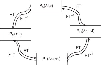
Figure 3.24 gives the relationship between the different system functions for a WSSUS channel.
Figure 3.24 System functions of a WSSUS channel.
3.6 Coherence Functions
The channel function ![]() in Figure 3.24 is commonly used to define two correlation functions – namely the frequency correlation function and the time correlation function:
in Figure 3.24 is commonly used to define two correlation functions – namely the frequency correlation function and the time correlation function:
These two functions are obtained by setting either Δt or Δω to zero as in Equations (3.70a) and (3.70b) and enable estimation of the coherence bandwidth and the coherence time respectively. The frequency correlation function in Equation (3.70a) gives the degree of similarity between any two frequency components that are separated by Δω. As the frequency separation increases, the correlation decreases until at some frequency separation the frequency components become completely uncorrelated. Similarly, given any particular frequency component the time correlation function gives the degree of correlation at two different instants of time separated by Δt. As Δt increases, the correlation decreases. Figure 3.24 shows that setting Δt to zero in Ph(Δt,τ) and taking its FT gives the frequency coherence function in Equation (3.70a).
The degree of correlation is usually expressed by the normalized spaced frequency–spaced time function, given by [30]:
3.71 ![]()
Setting the time difference or the frequency difference to zero gives the normalized frequency correlation function and the time correlation function respectively, as in:
The frequency separation or the time separation at which the value in Equations (3.72a) and (3.72b) drops to 0.5 or to 0.9 is usually taken as a measure of coherence. The functions in Equations (3.72a) and (3.72b) are also called correlation coefficient functions. See Section 5.9.2 for further discussion of the coherence functions.
3.7 Power Delay Profile and Doppler Spectrum
Two other widely used functions are the power delay profile Ph(τ) function, obtained from either Ph(Δt,τ) by setting the time difference to zero or from PS(τ,ν) by summing the power contribution from all the Doppler shifted components. The second function is the Doppler power spectrum PS(ν), obtained from PS(τ,ν) by summing the contribution from all the multipath components along the time delay axis.
Figure 3.25 gives three examples of the delay Doppler function PS(τ,ν), the corresponding power delay profile and the Doppler spectrum functions obtained from measurements in the 2 GHz band with 16.7 ns time delay resolution and 1 Hz Doppler shift resolution. The delay Doppler plots can be summed along each axis separately to give the multipath structure versus time as in Figure 3.25d–f or the Doppler spectrum as in Figure 3.25g–i.
Figure 3.25 Multipath spread in time delay and in Doppler shift (a–c), in time delay only (d–f) and in Doppler shift only (g–i). Each column represents the same measurement in each of the three representations.
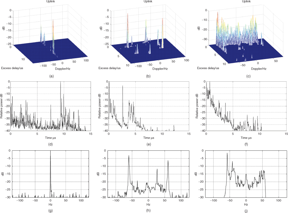
In Figure 3.25a the Doppler shift is zero due to both terminals and the environment being stationary and thus all the multipath components appear along the zero Doppler shift line. The lack of movement is also reflected in the corresponding Doppler spectrum in Figure 3.25g and in the power delay profile in Figure 3.25a, which is similar to the delay Doppler plot along the time axis. In Figure 3.25e, the delay profile shows two main components at zero time delay, ∼3 µs and a cluster between ∼4 and 5 µs. These are reflected in the Doppler spectrum in Figure 3.25h and the delay Doppler function in Figure 3.25b, which also shows three main components plus additional contributions from smaller components.
Figure 3.25c,f,i show a spread of power in both the time delay and in the Doppler shift. In particular, the first arriving cluster is seen to consist of a large number of multipath components, which are more evident from the delay Doppler plot than from the power delay profile. The delay Doppler function also permits resolution of the multipath components in a particular time delay according to their Doppler shift.
3.8 Parameters of the Power Delay Profile and Doppler Spectrum
3.8.1 First and Second Order Moments
Channel parameters that are related to the power delay profile and to the Doppler spectrum are the average value and the root mean square (RMS) obtained from the first order and second order moments respectively.
Considering the power delay profile in Figure 3.26, the average delay TD is given by the first moment of the power delay profile:
Figure 3.26 Power delay profile illustrating parameters for the computation of average delay and RMS delay spread.
where
![]()
In discrete form Equation (3.73a) can be rewritten as:
where j = 1 and M are the indices of the first and the last samples of the delay profile above the threshold level respectively and L is the index of the first received multipath component (first peak in the profile).
The RMS delay spread S is the square root of the second central moment and is given in Equation (3.74a) for the continuous time domain and in Equation (3.74b) for the discrete time domain:

Replacing the power delay profile in Equations (3.73a) and (3.73b) and in Equations (3.74a) and (3.74b) by the Doppler spectrum function Ps(ν) and τ by υ gives the corresponding average Doppler SD and RMS Doppler spread DS as given by:
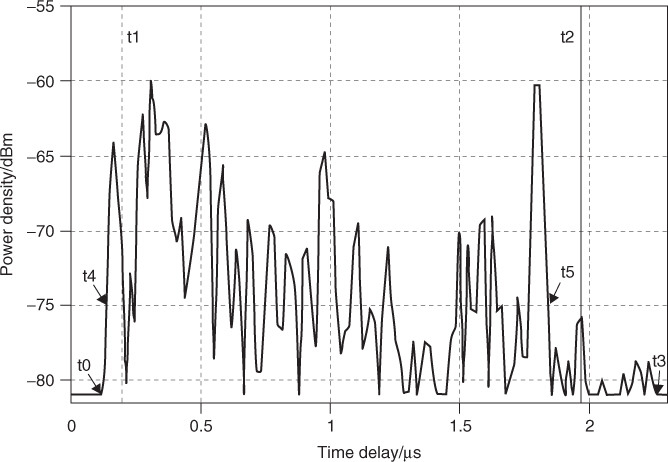
3.8.2 Delay Window and Delay Interval
Other parameters that can be estimated from the power delay profile are the delay window Wq and the delay interval Ith. The delay window is the length of the middle portion of the power delay profile containing a certain percentage, q, of the total power:
3.75a ![]()
where the boundaries t1 and t2 are defined by:
3.75b 
and the energy outside the window is split into two equal parts [(100 – q)/200]Pm.
The delay interval Ith is defined as the time difference between the instant t4 when the amplitude of the power delay profile first exceeds a given threshold Pth and the instant t5 when it falls below that threshold for the last time:
3.76 ![]()
3.8.3 Angular Dispersion
Derivation of the U-shaped Doppler spectrum assumes that the angular spread in the azimuth is uniformly distributed. This model does not always fit the measured channel characteristics.
Measurements of the received power versus angular spread can be used in a similar manner to estimate first and second order moments. The RMS angular spread σθ of the direction of arrival for a power density P(θ) in the direction θ where θ is in radians and is measured from the direction of the principal signal (assumed to be stationary within the duration of the measurement) is defined as:
where
3.77b 
and
All the integrals in Equations (3.77a–3.77c) are evaluated for values above the noise floor of the measurement.
3.9 The Two-Ray Model Revisited in a Stochastic Channel
The two-ray model was analyzed in Section 2.8 for both ionospheric propagation and for ground reflection in a terrestrial environment. In general the two-ray model can be applied to any environment using the tapped delay line model where only two taps with random variations are used. This results in the commonly used two-ray model given by:
3.78 ![]()
where A1 and A2 are independent and Rayleigh distributed, φ1 and φ2 are independent and uniformly distributed over the interval 0–2π and τ is the time delay separation between the two rays. By varying τ it is possible to examine a wide variety of frequency selective fading effects.
3.10 Multiple Input–Multiple Output Channels
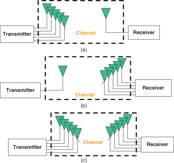
In a radio link multiple antennas can be employed at the transmitter and at the receiver. This gives three possible configurations: multiple input–single output (MISO), single input–multiple output (SIMO) and MIMO, as shown in Figure 3.27. SIMO configurations are used for a number of applications, which include diversity reception, estimation of the angle of arrival, forming a beam for reception in a particular direction (beam forming) and interference reduction. Similarly, MISO applications include transmitter diversity and beam forming at the transmitter end. The generalized multiple antenna systems, MIMO, have applications in beam forming at both ends of the radio link, capacity enhancement of the data rate in a limited bandwidth via parallel data transmission (spatial multiplexing) and double angular estimation of the multipath components, that is angles of departure at the transmitter and angles of arrival at the receiver.
Figure 3.27 Multiple antenna configurations: (a) MISO, (b) SIMO and (c) MIMO.
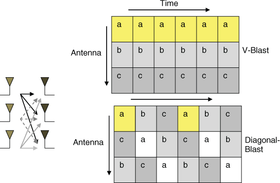
MIMO dates back to Jack Winters [31], who in 1987 proposed the configuration for communication between multiple mobiles and a base station (BS) with multiple antennas, as well as communication between two mobiles each with multiple antennas. The analytical basis of MIMO systems are presented by Foschini in [32–34], who proposed two suitable architectures for its realization known as vertical BLAST (Bell Labs layered space–time) and diagonal BLAST. In the BLAST system the data stream is divided into blocks, which are distributed among the transmit antennas. In vertical BLAST sequential data blocks are distributed among consecutive antenna elements, whereas in diagonal BLAST, they are circularly rotated among the antenna elements as illustrated in Figure 3.28 for the example of three transmit antennas. In vertical BLAST, data block ‘a’ is always assigned to antenna 1, data block ‘b’ to antenna 2 and data block ‘c’ to antenna 3. In diagonal BLAST, the data blocks assigned to antennas 1–3 in the first burst are [a b c], in the second burst [b c a] and in the third burst [c a b]. Thus diagonal BLAST offers the advantage of circulating the data blocks among the antennas, which avoids the same data block being transmitted over the same channel. However, this requires more processing power.
Figure 3.28 Vertical and diagonal Blast configurations [35].
Source: Wennstrom, M., Promises of Wireless MIMO Systems, http://www.signal.uu.se/courses/semviewgraphs/mw_011107.ppt. Reproduced with kind consent from the author.
In this section we first discuss the ideal channel properties for MIMO spatial multiplexing followed by the channel capacity equations.
3.10.1 Desirable Channel Properties for Narrowband MIMO Systems
Conceptually MIMO assumes that it is possible to transmit simultaneous data streams over the same bandwidth from different antennas. The data streams can then be recovered using a number of receive antennas if the propagation conditions are such that a number of orthogonal channels that correspond to the smaller number of transmit/receive antennas can be established.
MIMO is a narrowband concept where the assumption of flat fading holds; that is the bandwidth of transmission is within the coherent bandwidth of the channel and the frequency response can be considered a single-valued complex scalar. Thus the channel for n transmit by m receive antennas can be represented by a transmission matrix with complex coefficients of the form:
3.79 
where hij represents the channel coefficient between receiver antenna i and transmit antenna j.
Contrary to the single antenna configuration, multiple antenna systems aim to exploit the presence of multipath to enhance the data rate of transmission. For n transmit antennas and m receive antennas, the ideal channel conditions for MIMO transmissions are as follows [32]:
3.10.2 MIMO Capacity for Spatial Multiplexing
Under the ideal assumptions outlined in Section 3.10.1 the capacity equation for a MIMO system is given by:
where {·}H stands for the transpose of the complex conjugate (Hermetian transpose) and Im is the m × m unity matrix. Alternate expressions to Equation (3.80a) can be given in terms of the eigenvalues of the HHH, as:
where k ≤ min[n,m] is the rank of the matrix, which is ideally equal to the min(n, m) and λi is the ith eigenmode of HHH or in terms of the singular values ![]() as:
as:
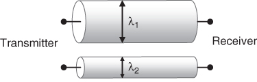
Equations (3.80b) and (3.80c) imply that it is possible to set up a number of independent channels between the transmitter and the receiver using the same bandwidth at the same time, each with its own gain factor λi, as illustrated in Figure 3.29.
Figure 3.29 Illustration of MIMO in terms of eigenvalues for equal power distribution [35].
Source: Wennstrom, M., Promises of Wireless MIMO Systems, http://www.signal.uu.se/courses/semviewgraphs/mw_011107.ppt. Reproduced with kind consent from the author.
When the product of the channel matrix with its complex transpose is an identity matrix, that is when all the eigenvalues are equal, which gives rise to orthogonal propagation conditions, Equation (3.80a) reduces to:
3.81a ![]()
Thus the capacity increases linearly with the smaller number of transmit–receive antennas. This in contrast to SISO channel's capacity, which increases logarithmically as the SNR increases, as given by [33]:
In Equation (3.82) |H|2 is the normalized channel power transfer function. For high SNR a 3 dB increase in ρ gives another bit/cycle capacity.
Since the capacity is a random variable, the corresponding ergodic capacity expressions are given as the expected value [36]:
3.83 ![]()
where ρ is the average received SNR at each branch. The ideal capacity of a MIMO system is then given by:
3.84 ![]()
which also increases linearly with n as in Equation (3.81b).
When the ideal channel matrix for optimum MIMO spatial capacity is not satisfied, it is possible to optimize the capacity via water filling where the transmitted power can be divided unequally with the good channels that have high eigenvalues, having more power, as shown in Figure 3.30. This technique relies on the receiver knowing the channel. Under these conditions the channel capacity is given by:
3.85 ![]()
Figure 3.30 Optimization of channel capacity via water filling [35].
Source: Wennstrom, M., Promises of Wireless MIMO Systems, http://www.signal.uu.se/courses/semviewgraphs/mw_011107.ppt. Reproduced with kind consent from the author.
where ϵi is a scalar representing the portion of available power to each transmitter such that all the transmitted power remains the same.
3.11 Capacity Limitations for MIMO Systems
A number of factors reduce the channel capacity from the ideal IID case described in Section 3.10.2. These include:
These effects result in a rank deficient channel matrix, which means that some columns in the channel matrix are linearly dependent. The information in these columns is redundant and is not contributing to the capacity of the channel. A channel matrix of rank 1 also results in the case of keyholes, even when the channel matrix is uncorrelated.
To distinguish the different types of MIMO channels depending on correlation the following classification proposed in [37] is adopted:
In the following sections we discuss the effects of these limiting factors on the channel capacity of MIMO systems including the relevant models.
3.12 Effect of Correlation Using Stochastic Models
Correlation of the channel matrix results from a small angular spread at the transmitter or at the receiver, small separation between antenna elements and the antenna geometry. The effect of correlation on channel capacity can be derived either analytically using certain correlation models, by simulation or experimentally.
Two types of MIMO models are available to study the effects of correlation: stochastic or nonphysical models and physical models. The nonphysical models are based on the channel statistical characteristics using nonphysical parameters. They are usually easy to simulate and can provide relatively accurate channel characterization. However, they do not give insight into the propagation characteristics of the MIMO channels and depend on the measurement equipment, such as the bandwidth, the configuration and aperture of the arrays, and the height and response of the transmit and receive antennas. In contrast, the physical models choose some crucial physical parameter to describe the MIMO propagation channel. Some typical parameters include angle of arrival, angle of departure and time of arrival. However, it is difficult to characterize the MIMO channel by a small number of parameters. In addition, the measurement equipment, such as antenna response and array configuration, affects the estimation of the channel parameters.
In this section we present MIMO capacity expressions based on stochastic modelling and some simple models to represent the correlation between the antenna elements. We then present the Kronecker stochastic model and discuss its limitations.
3.12.1 Capacity Expressions Based on Stochastic Correlation Models
To account for the correlation effects on the channel capacity, it is necessary to modify the channel matrix from the IID model. Two expressions are given below:
![]()
and
![]()
The mean capacity ![]() can then be obtained by taking the expected value of Equations (3.86a) and (3.86b):
can then be obtained by taking the expected value of Equations (3.86a) and (3.86b):
3.87 ![]()
If the correlation matrix R is separated into transmit and receive correlation matrices two separate channel capacities can be obtained, each dependent on the correlation effects at either end of the link. In this case the elements of the correlation matrix are given by:
![]()
![]()
In this case, the upper bound, which combines both covariance matrices, corresponds to the smaller capacity value:
3.12.2 Capacity Expressions Based on Uniform and Exponential Correlation Models
Two correlation models proposed in [40] and [41] to estimate the channel capacity of a linear array with correlated elements are presented here:
3.90 ![]()
Simulation of capacity estimates based on the uniform correlation coefficient model with r = 0.5 gave an upper bound capacity in Equation (3.88) of 40 bits/s/Hz at 30 dB SNR for 10 transmit and 10 receive antennas [39]. This figure is reduced by whichever side (transmit or receive) has the higher correlation coefficient. For 100 % correlation at one end and 0 % correlation at the other end, the capacity drops down to 10 bits/s/Hz. In the simulations the channel is assumed to be correlated Rayleigh with correlation at both ends and the components of the channel matrix H are identically distributed correlated complex Gaussian variables.
Simulation results using the exponential model for n = 10, 50 and SNR of 30 dB show that: (i) the MIMO capacity decreases for r > 0.5–0.8 and for r > 0.8 the capacity rapidly declines, (ii) the accuracy of the model decreases as the SNR and n decrease and (iii) C is about 50 bits/s/Hz for n = 10 and r ≅ 0.75 [40].
Measurements in [42] confirm the application of the exponential model at the transmitter end and the uniform model at the receiver end.
3.12.3 The Kronecker Stochastic Model
The IST SATURN (Information Society Technologies – Smart Antenna Technology in Universal Broadband Wireless Networks) project [43, 44] proposed an overall channel model based on the Kronecker product of the covariance matrices from both the transmitter end ![]() and the receiver end
and the receiver end ![]() . This is a narrowband model where the (nm) × (nm) channel covariance matrix RH, which contains the complex correlation between all the (nm) elements of the n × m channel matrix H is given by:
. This is a narrowband model where the (nm) × (nm) channel covariance matrix RH, which contains the complex correlation between all the (nm) elements of the n × m channel matrix H is given by:

where hi is the ith row of H, hj is the jth column of H, vec( ) denotes the vector operator stacking all elements of a matrix column-wise into a single vector, ![]() is the Kronecker product, E{} is the expected value and T is the transpose of the matrix.
is the Kronecker product, E{} is the expected value and T is the transpose of the matrix.
In [45], Equation (3.92) is shown to lead to a channel matrix as given by:
3.93 ![]()
where G is a stochastic n × m matrix with IID CN(0,1) elements and the square root means that the square root of the matrix multiplied by its complex transpose gives the original matrix.
The Kronecker model is derived under the following assumptions [46]:
Measurements with 8 × 8 antenna arrays show that the Kronecker model underestimates the channel capacity in both a correlated multipath channel and in an indoor non-LOS environment [47]. This is attributed to the failure of the model to render the multipath structure correctly.
3.13 Correlation Effects with Physical Channel Models
Physical MIMO channel models are based on the physical parameters of the channel, such as distribution of the multipath components, their angular spread at the transmitter and at the receiver, antenna element spacing and antenna array geometry. In this section we study the various effects and relevant models pertaining to antenna separation, angle of arrival and angle of departure, starting with the distributed scattering model, and then considering the single ring and the double ring models. We then briefly review the COST 259 model and its extension to the multidimensional parametric channel model.
3.13.1 Distributed Scattering Model
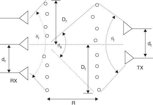
The scattering model proposed in [37] is based on linear arrays being deployed at the transmitter and at the receiver, with interelement spacing equal to dt and dr respectively. The model assumes scatterers at both ends with a dimension from the centre of the array, equal to Dt and Dr respectively, as illustrated in Figure 3.31. The angle spread at the transmitter, at the receiver and at the scatterers are θt, θr and θs respectively.
Figure 3.31 Illustration of the distributed scatterer model [48].
Source: Yu, K. and Ottersten, B., (November, 2002) Models for MIMO propagation channels, A review, Wiley Journal on wireless communications and mobile computing, special issue on adaptive antennas and MIMO systems, DOI: 10.1002/wcm, 78IR-S3_SB-0223. Reproduced with permission from John Wiley & Sons, Ltd.
In this model, the channel matrix is represented by [37]:
where:
In addition to the keyhole effect, Equation (3.95) shows that the channel matrix can become rank deficient if any of the transmit or the receive correlation matrices become rank deficient. This can occur if the angular spread is small, which results in loss of antenna diversity and spatial multiplexing capacity leaving only the antenna gain. Also, if the scatterers are absent at one end of the link the rank at that end is governed by the antenna separation. Equation (3.95) also shows that in the absence of correlation at both ends of the link and when the scatterer matrix leads to a full rank matrix, the product of the IID matrices Gr and Gt approaches a single Rayleigh matrix.
Monte Carlo ray tracing simulations performed to verify the model show that as the range R is increased the channel goes from UHR to ULR, illustrating the effect of the scatterers on the capacity.
In [48] it is proposed that for the non-LOS case a full rank matrix can be obtained if:
Equation (3.95) predicts that the high rank region starts at 23 m of scattering radius for a 10 km range, with three transmit and three receive antennas, 10 dB SNR and dt = dr = 3λ, where λ is equal to 0.15 m at 2 GHz.
3.13.2 Single-Ring Model
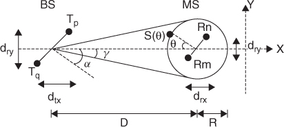
The single-ring scatterer model [48] is based on the assumption that the BS is elevated and hence not surrounded by scatterers whereas the mobile station (MS) is surrounded by buildings with no direct LOS. Thus the receiver array is surrounded by K scatterers S(θ), which are uniformly distributed over [−π, π) and IID in θ within a single ring of radius R, as illustrated in Figure 3.32. In the figure, D represents the distance between the BS and the MS, α is the AOA at the BS and γ is the angle spread, and since D and R ![]() spacing between the antenna elements,
spacing between the antenna elements, ![]() . The model further assumes that each ray is reflected once and arrives at the receiver with equal power.
. The model further assumes that each ray is reflected once and arrives at the receiver with equal power.
Figure 3.32 The single-ring scattering model [48].
Source: Yu, K. and Ottersten, B., (November, 2002) Models for MIMO propagation channels, A review, Wiley Journal on wireless communications and mobile computing, special issue on adaptive antennas and MIMO systems, DOI: 10.1002/wcm, 78IR-S3_SB-0223. Reproduced with permission from John Wiley & Sons, Ltd.
For this model the channel coefficients between the pth transmit antenna and the nth receive antenna are given by:
3.96 ![]()
where ![]() denotes the distance between X and Y and λ is the wavelength. When the number of scatterers is large, the channel coefficients are Gaussian and the covariance between Hp,n and Hq,m is given by:
denotes the distance between X and Y and λ is the wavelength. When the number of scatterers is large, the channel coefficients are Gaussian and the covariance between Hp,n and Hq,m is given by:
3.97 ![]()
Simulations for fixed wireless access using the single ring scattering model [49] show the following properties of the model:
A model that is related to the single-ring model is the von Mises angular distribution model, which uses the PDF of the angular spread at the mobile and takes the Doppler spread into account [48]. An important advantage of using the von Mises angular distribution is that it gives a closed form expression and therefore can be used to study the channel covariance analytically.
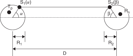
3.13.3 Double-Ring Model
In the two-ring model both the BS and the MS are surrounded by scatterers as illustrated in Figure 3.33, which can be the case for indoor wireless communications. In this case the rays are reflected twice and there is a possibility that the signals reflected by the scatterers at the transmitter and at the receiver are not independent. Therefore the channel covariance matrix cannot completely describe the MIMO channel. The channel coefficients are now given by the following equation, where K1 and K2 are the number of scatterers in the two rings [48]:
3.98 
Figure 3.33 Illustration of the two-ring model [48].
Source: Yu, K. and Ottersten, B., (November, 2002) Models for MIMO propagation channels, A review, Wiley Journal on wireless communications and mobile computing, special issue on adaptive antennas and MIMO systems, DOI: 10.1002/wcm, 78IR-S3_SB-0223. Reproduced with permission from John Wiley & Sons, Ltd.
3.13.4 COST 259 Models
The COST 259 model is a double-directional model developed by the European cooperative research initiative COST 259 [50]. It takes the direction of departure (angle of departure, AOD) at the transmitter and the direction of arrival (angle of arrival, AOA) at the transmitter in addition to the time delay. Assuming L plane waves impinging at the receiver, the double-directional channel impulse response is defined as:
3.99 
where r is the location of the receiver with respect to the transmitter, τ is the time delay and ![]() and
and ![]() are the AOD and AOA respectively.
are the AOD and AOA respectively.
3.13.5 Multidimensional Parametric Channel Model
The parametric channel model is an extension of the COST 259 model where a finite number of multipath components are assumed to connect the transmitter and the receiver and each component is characterized by a number of parameters. These include the time delay τ, the Doppler shift ν, the angles of departure in azimuth and in elevation ![]() and similarly the angles of arrival in azimuth and in elevation
and similarly the angles of arrival in azimuth and in elevation ![]() , as expressed by [51]:
, as expressed by [51]:
3.100 
where ![]() represents the 2 × 2 path weight matrix describing the two polarization responses of the receive and transmit antennas respectively, given by [51]:
represents the 2 × 2 path weight matrix describing the two polarization responses of the receive and transmit antennas respectively, given by [51]:
3.101 ![]()
Using the parameters of the multipath components, the received signal at each antenna can be estimated where it is assumed that the amplitude variations across the array are insignificant and that the wave has an additional phase shift depending on the location of the element within the array. The MIMO channel coefficients can then be estimated to evaluate the capacity.
3.13.6 Effect of Antenna Separation, Antenna Coupling and Angular Spread on Channel Capacity
The effect of separation between antenna elements in an array affects the correlation between the antenna elements. In [52] the channel capacity of a MIMO system has been shown not to be affected by the correlation between the receive antenna elements of a ULA provided the following conditions are satisfied:
3.102 ![]()
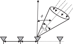
Figure 3.34 Incoming multipath signals arrive to the linear antenna array within ±Δ of the mean angle φ [52].
Source: Loyka, S., and Tsoulos, G., (2002) Estimating MIMO system performance using the correlation matrix approach, IEEE Communications Letters, vol. 6., No. 1, pp 19–21. Reproduced with permission IEEE.
Using simulations to estimate the channel capacity assuming 20 multipath components, 10 element transmit and receive arrays, and 30 dB SNR, the maximum channel capacity occurs for the broadside case with high angular spread. For an angular spread of about 10°, mean capacities of ∼55 bits/s/Hz are achieved for an antenna separation on the order of 2.5 wavelengths whereas for an angular spread of 1° the required separation is about 27 wavelengths.
Simulations to study the effect of antenna separation on the achieved capacity of a 16 × 16 MIMO channel with linear arrays as in Figure 3.34 using both a uniform distribution and a Gaussian distribution for the AOA with 2° RMS angular spread show that for 10 dB SNR for both single and dual polarizations [38]:
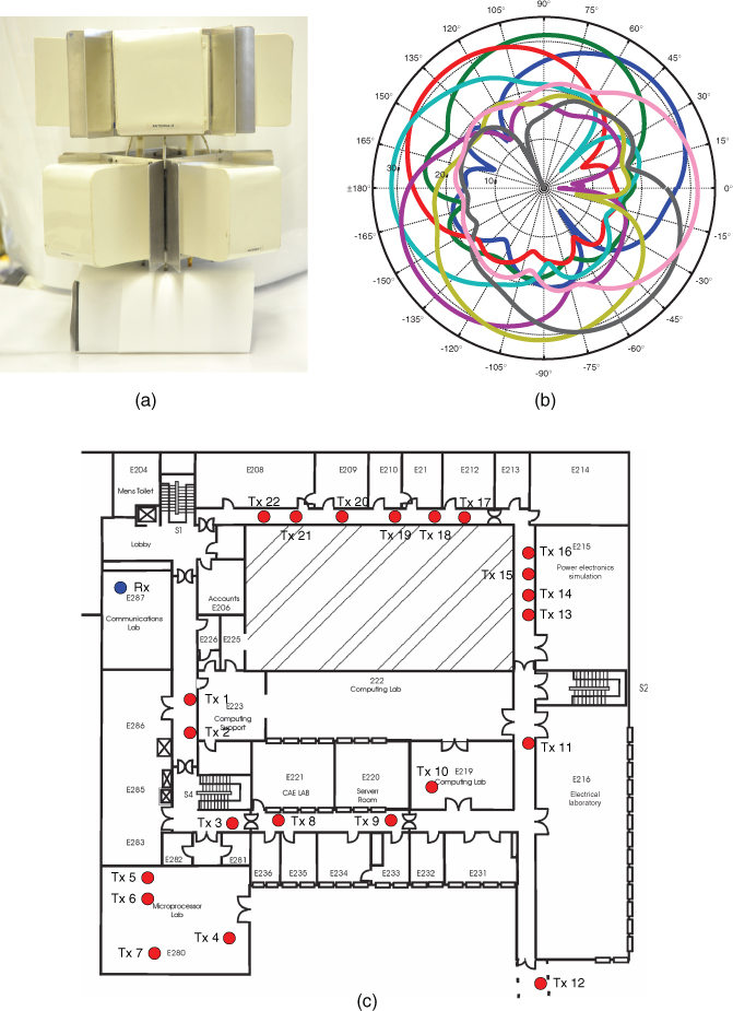
Using circular uniform beam arrays (CUBAs) with six elements at the transmitter and eight elements at the receiver, as illustrated in Figure 3.35a,b for the eight element array, the effect of angular spread at the transmitter (angle of departure) and at the receiver (angle of arrival) on channel capacity can be computed from wideband measurements as illustrated in Figure 3.35c for an indoor environment [53]. In such an environment the RMS angular spread for the angle of departure/angle of arrival and the mean RMS angular spread are of similar order (68.5° for the angle of departure) and (69.7° for the angle of arrival). Although the angular spread values are relatively significant, the correlation coefficient between the capacity and the RMS angular spread is on the order of 0.65 at the transmitter and 0.41 at the receiver, which is less obvious than for the simulated wireless access scenarios.
Figure 3.35 (a) Eight element CUBA array used at the receiver in indoor MIMO measurements and (b) its radiation pattern and (c) layout of the measurement environment [53]. Source: Razavi-Ghods, N., and Salous S., (2009), Wideband MIMO channel characterization in TV studios and Radio Sci., 44, RS5015, doi:10.1029/2008RS004095. Reproduced in accordance with guidlines from Radio Science.
3.13.7 Effect of Mutual Coupling
For a particular environment appropriate choice of antenna separation between elements in an MIMO array is important for the realization of channel capacity. Large antenna separation requires considerable space on the user unit or the ability to place as many antennas as possible in a small space with possibly different polarizations. Close spacing of the antenna elements increases the coupling between antennas and makes it difficult to match the antenna impedance for efficient energy transfer from the antenna to a receiver or from a transmitter to the antenna. The amount of mutual coupling is a function of the spacing between elements, the number of antennas in the array and the direction of each ray relative to the array plane.
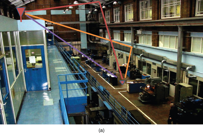
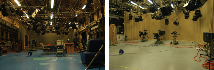
Two opposing views are postulated with regard to the effect of mutual coupling on correlation. Generally it is assumed that coupling increases correlation. However, using simulations with a dipole array and the single scattering ring model the effect of mutual coupling is shown to reduce the correlation between the elements and hence to improve the MIMO capacity [54]. It is proposed that the coupling phenomenon decorrelates the signals by acting as an additional ‘channel’ whereas, for the case of rich IID, coupling will degrade the performance. Measurements collected at 10 different locations in the TV studio shown in Figure 3.36 with antenna spacing equal to λ/3, λ/2, λ and 3λ/2 show an increase in capacity as the antenna element separation is increased. Compared to λ/2 antenna spacing the capacity is on average reduced for the λ/3 spacing by 2 bits/s/Hz [53]. This is consistent with the comment that coupling reduces the capacity in the case of IID channels [54].
Figure 3.36 Environment of TV studios [53]. Source: Razavi-Ghods, N., and Salous S., (2009), Wideband MIMO channel characterization in TV studios and Radio Sci., 44, RS5015, doi:10.1029/2008RS004095. Reproduced in accordance with guidelines from Radio Science.
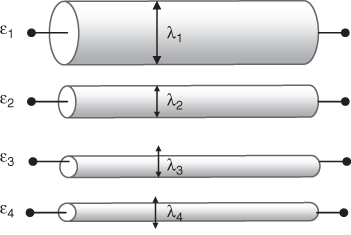
Experimental results of correlation as a function of antenna type and antenna separation conducted over an HF radio link in the UK between Durham and Bruntingthorpe are shown in Figure 3.37 [55]. The radio link is shown in Figure 3.37a with the antenna array geometry in Figure 3.37b, which consists of five monopole antennas, one loop antenna and two crossed wire antennas in conjunction with an eight channel receiver. The transmit array consists of two pairs of orthogonally oriented inverted ‘V’ wire antennas spaced approximately 22 m apart (centre-to-centre distance) in the directions of an E–W and N–S arm. Simultaneous CW transmissions are enabled via a 10 Hz frequency offset between the different antenna elements. The total frequency range covered in the transmission is sufficiently small to avoid frequency selectivity. This is verified by transmitting all four frequencies first from the same antenna where all the received signals from the four frequencies are identical.
Figure 3.37 (a) Geometry of the HF link between Durham and Bruntingthorpe, (b) layout of antenna array, (c) correlation coefficient as a function of antenna separation and (d) capacity estimates for different array sizes ranging from 2 × 2 to 4 × 4 [55]. Source: Gunashekar, S.D., Warrington, E.M., Salous, S. et al. (2009) Investigations into the feasibility of multiple input multiple output techniques within the HF band: preliminary results. Radio Sci., 44, RS0A19. doi:10.1029/2008RS004075.
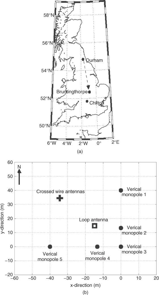
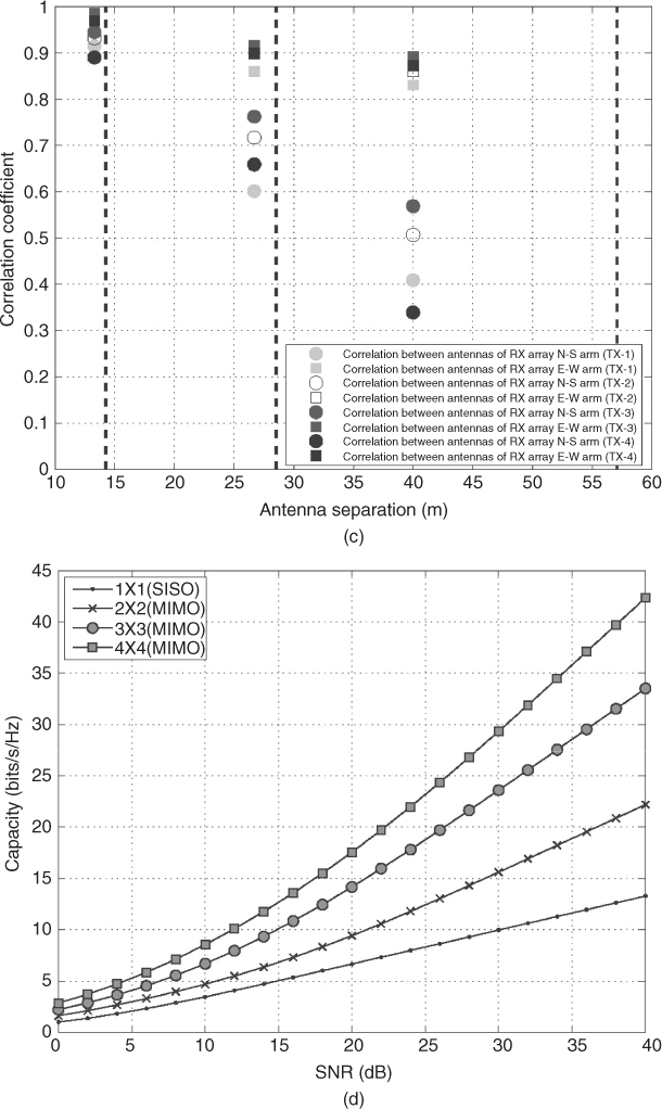
The effect of antenna spacing on the correlation coefficient is shown in Figure 3.37c where the correlation is seen to decrease as the antenna separation increases and it is also seen to vary with the orientation of the element. The resulting capacity for the different number of antenna combinations ranging from SISO capacity to 4 × 4 is shown in Figure 3.37d.
Table 3.2 gives the correlation coefficient between pairs of transmitters at each receive antenna. The orientation of the transmit (TX) antennas and receive (RX) antennas, is as follows: TX-1, E–W arm of crossed inverted V wire array 1, TX-2, N–S arm of crossed inverted V wire array 1; TX-2; RX-1, vertical whip 1 (N–S arm); RX-2, vertical whip 2 (N–S arm); RX-3, vertical whip 3 (N–S/E–W arms); RX-4, vertical whip 4 (E–W arm); RX-5, vertical whip 5 (E–W arm); RX-6, large loop antenna (E–W orientation); RX-7, N–S arm of crossed inverted V wire array; RX-8, E–W arm of crossed inverted V wire array. The correlation coefficient is again seen here to be a function of the orientation of the elements with respect to each other and the propagation path.
Table 3.2 Correlation coefficient between different antenna pairs at each receiver [55]
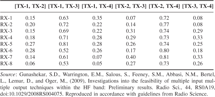
Source: Gunashekar, S.D., Warrington, E.M., Salous, S., Feeney, S.M., Abbasi, N.M., Bertel, L., Lemur, D., and Oger, M., (2009), Investigations into the feasibility of multiple input multiple output techniques within the HF band: Preliminary results. Radio Sci., 44, RS0A19, doi:10.1029/2008RS004075. Reproduced in accordance with guidelines from Radio Science.
Since MIMO can require significant spacing between the elements, which in the HF band translates into large areas due to the wavelength, colocated antenna arrays such as the X–Y–Z loop array, which consists of three orthogonal loops, and the ground symmetric loop (GSL) array, which is a three-element antenna array consisting of three loops placed symmetrically with respect to the ground, as shown in Figure 3.38, can be a viable alternative to spatial arrays. Using the X–Y–Z antenna array and a single active square loop antenna (side length 1 m) at a distance of approximately 22 m at the receive end over the same path in the UK, Figure 3.38 shows that capacity gains are still achievable with such antennas [56]. Table 3.3 gives the correlation coefficient between different receive pairs with different transmit elements where the correlation coefficient is generally seen to be ≤0.82.
Figure 3.38 (a) X–Y–Z loop antenna array [60], (b) Giselle antenna array [54] and (c) capacity with X–Y–Z array and inverted V array [60].
Source: Gunashekar, S.D., E.M. Warrington, S.M. Feeney, S. Salous, and N.M. Abbasi (2010), MIMO communications within the HF band using compact antenna arrays. Radio Sci., 45, RS6013, doi:10.1029/2010RS004416. Reproduced in accordance with guidelines from Radio Science.
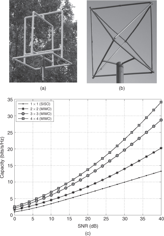
Table 3.3 Correlation coefficient between different antenna elements [60]
| Receiving antenna Paris being correlated | Transmitter | Mean correlation coefficient |
| X–Y–Z array: N–S and E–W loops | TX-1 | 0.58 |
| TX-2 | 0.42 | |
| X–Y–Z array: N–S and horizontal loops | TX-1 | 0.40 |
| TX-2 | 0.33 | |
| X–Y–Z array: E–W and horizontal loops | TX-1 | 0.81 |
| TX-2 | 0.77 | |
| GSL array: loops 1 and 2 | TX-1 | 0.81 |
| TX-2 | 0.72 | |
| GSL array: loops 1 and 3 | TX-1 | 0.79 |
| TX-2 | 0.70 | |
| GSL array: loops 2 and 3 | TX-1 | 0.48 |
| TX-2 | 0.39 | |
| Colocated N–S and E–W inverted V long wire antenna | TX-1 | 0.82 |
| TX-2 | 0.72 |
Source: Gunashekar, S.D., E.M. Warrington, S.M. Feeney, S. Salous, and N.M. Abbasi (2010), MIMO communications within the HF band using compact antenna arrays. Radio Sci., 45, RS6013, doi:10.1029/2010RS004416. Reproduced in accordance with guidelines from Radio Science.
3.14 Effect of Number of Scatterers on Channel Capacity
The fundamental concept of MIMO capacity is based on the presence of a large number of multipath components whereby the channel between the different antenna elements at the transmitter and at the receiver can be considered IID. In the presence of a limited number of multipath components, the channel capacity is reduced as discussed in [56–59], where it is shown that the rank of the channel matrix and hence the channel capacity are limited by this number, as given by:
3.103 ![]()
where ns is the number of scatterers, m is the number of receive antennas and ζi is the gain of the ith multipath component.
To illustrate the effect of the number of multipath components we start by considering free space propagation and follow this by examples from HF propagation where the number of multipath components is generally limited.
3.14.1 Free Space Propagation
In free space propagation there is only the LOS component. Under such a scenario, also named the green field, the coefficients of the channel matrix are in the form of [56]:
3.104 ![]()
where Ti and Rk are the coordinate vectors for the antenna elements, T1 and R1 are the reference locations so that H1,1 = 1 and the absolute attenuation need not be calculated.
If the antenna separation is less than half a wavelength for both the transmitter and the receiver antenna arrays, the channel coefficients are all equal since the phases are nearly the same; that is the spatial signature is imposed by the phase of the array. When the phase difference between consecutive elements approaches 0 the channel matrix approaches the all 1 matrix and therefore has rank 1 and the capacity gain is essentially due to the n-fold array gain. Hence the channel capacity reduces to:
3.105a ![]()
For large separation between antenna elements, the amplitude of the coefficients are the same but the phases are different, which can give HHH = nIn, resulting in a LOS matrix of rank n, giving a channel capacity as:
The capacity equation in Equation (3.105b) is seen to hold for the following antenna geometry:
In [49] it is shown that as the range R between the transmitter and the receiver decreases, linear independence between the signatures starts to build up and for orthogonality to hold the condition in the following equation must be satisfied:
3.106 ![]()
where dt and dr refer to the antenna separation at the transmitter and at the receiver respectively and M is the number of receive antennas. In a pure LOS situation orthogonality can only be achieved for very small values of R. For example, at 2 GHz with M = 3, a maximum value of R = 20 m is acceptable for 1 m antenna spacing.
Simulations at 2.154 GHz for 20 dB SNR show that a mean capacity of 19 bits/s/Hz can be achieved for a LOS street canyon scenario [57]. The simulations assume a street width of 40 m, 4 × 4 antenna configuration with antenna spacing of half a wavelength at both ends, an MS antenna height of 1.8 m, a base station antenna height of 15 m located at a distance of a quarter of the street width from a wall with relative permittivity equal to 15 while the MS is moved from 100 m to 120 m from the BS in steps of 0.01 m. As the street width is increased the capacity approaches that of free space and the capacity gain is due to antenna diversity. For walls with higher permittivity the capacity also increases since the reflected components have comparable power to the LOS component. In addition, the mean capacity is also shown to increase for reflections on the order of up to 5. The simulations do not take the street crossings into account and assume the street walls to be flat smooth surfaces.
3.14.2 Limited Number of Multipath Components
The effect of the number of multipath components on the correlation coefficient at the transmit and receive arrays and the resulting capacity can be studied over HF skywave radio links as the ionosphere normally supports a limited number of multipath components, which vary with the time of day, season and sunspot cycle. Here we present examples of capacity estimates from measurements performed at 5.255 MHz with 2 × 8 arrays over the HF link shown in Figure 3.37a between 12:48 UT and 14:29 UT in January 2009 [60]. The arrays used in the measurements consisted of two colocated orthogonal end-fed inverted V long wire antennas at the transmitter and a number of colocated antenna arrays at the receiver. These included: an array consisting of end-fed, crossed inverted V wire antenna array, an active crossed dipole antenna array as shown in Figure 3.39, the X–Y–Z array of Figure 3.38a and the GSL array of Figure 3.38b. Vertical ionograms in Figure 3.40a and b obtained from Chilton at 12:50 and 14:20 show the change in the propagation modes present during the transmission. Figure 3.41 displays the results for a total of 69 records each consisting of 1 minute data. The figure shows the variations in the number of multipath components and the corresponding correlation at the receiver and at the transmitter and the resulting capacity for 30 dB SNR for various MIMO configurations (2 × 2, 2 × 3, 2 × 4, 2 × 5). The increase in correlation coefficient and the decrease in capacity is seen to be directly correlated to the number of multipath components. The existence of a greater number of propagation paths has resulted in lower correlation coefficient and thus a higher capacity. Specifically, the majority of the correlation coefficient values are below 0.4 and never exceed 0.8 during the period, which had five multipath components, while for the period with two multipath components the correlation almost always exceeds 0.8. The capacity is also seen to increase as the number of receive antennas is increased due to diversity gain.
Figure 3.39 Crossed dipole array [60].
Source: Gunashekar, S.D., E.M. Warrington, S.M. Feeney, S. Salous, and N.M. Abbasi (2010), MIMO communications within the HF band using compact antenna arrays. Radio Sci., 45, RS6013, doi:10.1029/2010RS004416. Reproduced in accordance with guidelines from Radio Science.
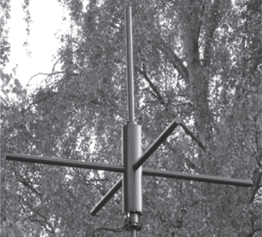
Figure 3.40 Vertical ionograms obtained at Chilton (a) at 12:50 and (b) at 14:20 [60].
Source: Gunashekar, S.D., E.M. Warrington, S.M. Feeney, S. Salous, and N.M. Abbasi (2010), MIMO communications within the HF band using compact antenna arrays. Radio Sci., 45, RS6013, doi:10.1029/2010RS004416. Reproduced in accordance with guidelines from Radio Science.
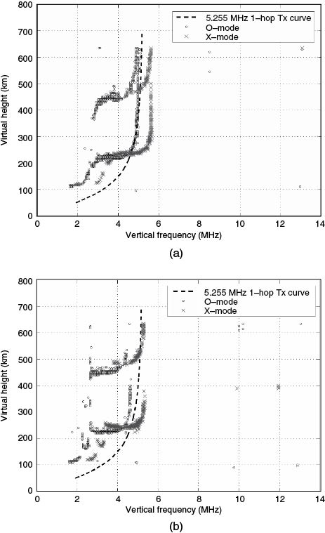
Figure 3.41 Results of measurements over HF skywave link: (a) number of multipath components, (b) correlation coefficient between receive elements, (c) correlation coefficient between transmit elements and (d) capacity for 30 dB SNR [60].
Source: Gunashekar, S.D., E.M. Warrington, S.M. Feeney, S. Salous, and N.M. Abbasi (2010), MIMO communications within the HF band using compact antenna arrays. Radio Sci., 45, RS6013, doi:10.1029/2010RS004416. Reproduced in accordance with guidelines from Radio Science.
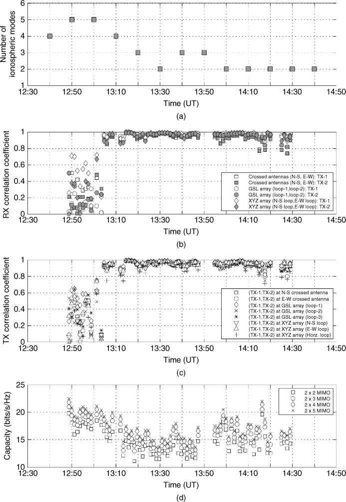
Figure 3.42 presents plots of amplitude against time for a period of approximately 60 seconds commencing at 12:59 UT, which coincides with the period that had five multipath components, for each of the three loops comprising the GSL array. Deep amplitude fading is observed, consistent with the existence of multiple propagation paths, and the fades occur at different times on all three antennas. This results in the low values of correlation coefficient. Figure 3.43 depicts the amplitude patterns observed for a similar period at 13:46 UT on the three loops comprising the GSL array. In general, compared with the data in Figure 3.42, significantly less variations in signal amplitude are observed, which is indicative of a reduction in the number of ionospheric modes. The fades also occur at approximately similar times, which give rise to the high correlation coefficients.
Figure 3.42 Amplitude (in linear units) over 60 s at 12:59 UT on 29 January 2009, on the three loops of the GSL array during a 2 × 8 measurement campaign between Durham and Bruntingthorpe. Transmission consisted of CW signals offset by 10 Hz on crossed inverted V wire antenna array [60].
Source: Gunashekar, S.D., E.M. Warrington, S.M. Feeney, S. Salous, and N.M. Abbasi (2010), MIMO communications within the HF band using compact antenna arrays. Radio Sci., 45, RS6013, doi:10.1029/2010RS004416. Reproduced in accordance with guidelines from Radio Science.
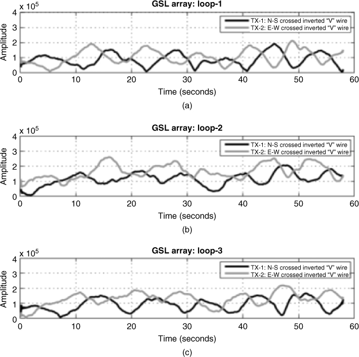
Figure 3.43 Amplitude (in linear units) over 60 s at 13:46 UT on 29 January 2009, on the three loops of the GSL array during a 2 × 8 measurement campaign between Durham and Bruntingthorpe. Transmission consisted of CW signals offset by 10 Hz on crossed inverted V wire antenna array [60].
Source: Gunashekar, S.D., E.M. Warrington, S.M. Feeney, S. Salous, and N.M. Abbasi (2010), MIMO communications within the HF band using compact antenna arrays. Radio Sci., 45, RS6013, doi:10.1029/2010RS004416. Reproduced in accordance with guidelines from Radio Science.
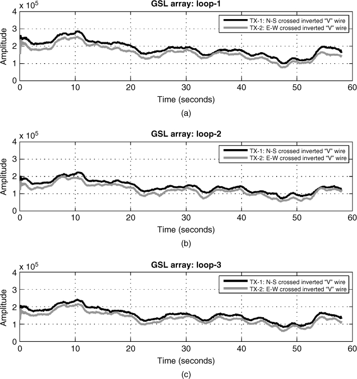
3.15 Keyholes
A keyhole refers to the case when the channel matrix is rank deficient, even when the matrix is uncorrelated [61–63]. For example, if the channel matrix is of the form given in:
3.107 ![]()
the determinant of H is equal to zero and the channel only gives one degree of freedom instead of two, which are necessary to extract the two data streams. The entries in the channel matrix are no longer Gaussian distributed but each is the product of complex Gaussian distributions resulting in Bessel functions.
A keyhole situation arises when, for example, there is a metal screen between the transmitter and the receiver with a hole – hence keyhole (see Figure 3.44). For indoor environments keyholes might arise in propagation in a hallway, which corresponds to single-mode guided propagation. For outdoor environments diffraction over rooftops in the vicinity of the mobile or a tunnel might cause the keyhole effect. In [63] it is argued that the rooftop diffracting edge acts as an equivalent horizontal line source with varying current strength along its length. If the base antennas are vertically separated, the richness of the perceived channel is collapsed and a keyhole is formed. Increasing the vertical antenna separation does not remedy the situation but placing the antenna elements in a horizontal array with adequate separation might.
Figure 3.44 Illustration of keyhole transmission.
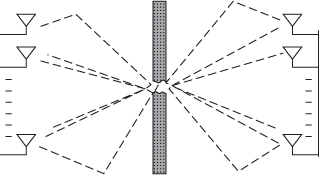
It has also been suggested that using horizontal polarization antennas can reduce the effect of a keyhole whereas in [63] cross polarization coupling has been reported to be −6 dB and the fading on the two polarizations has been found to be uncorrelated. Thus capacity figures can be expected to double when dual polarization is used at both the transmitter and at the receiver.
3.16 Rician Channels
The effect of the Rician channel on MIMO capacity can be studied by dividing the channel coefficients into two parts as in the following equation, where one corresponds to the LOS and the other to the Rayleigh fading component [56, 64, 65]:
3.108 ![]()
with a2 + b2 = 1 and the Rician factor K = a2/b2.
Simulations with different values of K show that when the antenna spacing is less than a wavelength, the capacity reduces to that of the LOS with one degree of freedom (rank 1). However, if an array geometry is used as discussed in Section 3.14.1 for the case of free space propagation, such that the channel matrix is of rank n, the capacity increases with increasing K. High capacities for Rician channels can be obtained by spreading out the elements of the array either explicitly by transmitting from different locations or implicitly by adding reflectors to create images.
In [64] the channel matrix was divided into a fixed LOS component and a Rayleigh component to carry out simulations for a 2 × 2 MIMO channel:
3.109 
where Xij are correlated zero-mean, unit variance, complex Gaussian random variables of the Rayleigh matrix Hv, exp(jφij) are the elements of the fixed matrix HF, αi are the factors due to cross polarization and cross polarization discrimination (XPD) and K is the temporal Ricean K factor.
An example of the effect of the presence of the LOS component is given in Table 3.4, which gives the mean capacity for the measurements in the TV studio environment of Figure 3.36. The results in the table show that the obstructed line of sight (OLOS) gives considerably higher capacity values than the LOS channel.
Table 3.4 Channel capacity in TV studio environment of Figure 3.36 illustrating the effect of a Rician channel [53]
| Antenna configuration | Mean capacity (bits/s/Hz) |
| BBC 2 × 2 LOS | 11.7 |
| BBC 2 × 2 OLOS | 16.3 |
| BBC 4 × 4 LOS | 19.13 |
| BBC 4 × 4 OLOS | 30.52 |
Source: Razavi-Ghods, N., and Salous S., (2009), Wideband MIMO channel characterization in TV studios and Radio Sci., 44, RS5015, doi:10.1029/2008RS004095. Reproduced in accordance with guidelines from Radio Science.
3.17 Wideband MIMO Channels
Since MIMO is a narrowband concept, the wideband capacity is computed by dividing the frequency band into N narrower (frequency-flat) subchannels denoted as Hi (i = 1, 2,…, Nf), where each subchannel has n × m coefficients for an n × m MIMO system. This gives an MIMO channel denoted by:
In Equation (3.110) Hi is the n × m channel matrix for the ith frequency component. As in the case of narrowband channels, when the channel is unknown to the transmitter, equal power is allocated to each transmit antenna and the resulting capacity is the average over all the frequency bands given either in terms of the sum:
3.111a ![]()
or in terms of the integral [66]:
3.111b ![]()
where H(f) is the frequency selective response and B denotes the bandwidth of interest, where ρ denotes the average SNR and Hi is the n × m matrix containing the sampled channel frequency responses for each of the subchannels.
For a frequency selective MIMO channel, the ergodic capacity is defined as:
3.112 ![]()
Prior to the computation of the channel capacity, the MIMO channel matrix data are normalized to remove the absolute power bias. This enables the comparison of capacity estimates in different environments. In [67] it is proposed to normalize the channel matrices so that the Frobenius norm is equal to nm, which gives an average SISO gain of one. Normalization of each individual sampled channel matrix to have an SISO gain of one assumes some form of power control, which allows the receiver to always have the same SNR, regardless of path loss. A more practical approach estimates an average of one over all SISO gains, thus assuming an average SNR. If β represents the normalization constant for each time snapshot and fi represents the frequency sample index, the specified unity power gain constraint may be expressed as [67]:
3.113 ![]()
Solving for β gives:
3.114 
Figure 3.45 gives an example of a wideband MIMO channel for a 4 × 4 discone antenna configuration obtained over 240 MHz bandwidth in the TV studio environment of Figure 3.36 and the computed channel capacity for different antenna combinations.
Figure 3.45 (a) Discone antenna array and (b) capacity estimates versus SNR used in the TV studio measurements [55]. Source: Gunashekar, S.D., Warrington, E.M., Salous, S., Feeney, S.M., Abbasi, N.M., Bertel, L., Lemur, D., and Oger, M., (2009), Investigations into the feasibility of multiple input multiple output techniques within the HF band: Preliminary results. Radio Sci., 44, RS0A19, doi:10.1029/2008RS004075. Reproduced in accordance with guidelines from Radio Science.
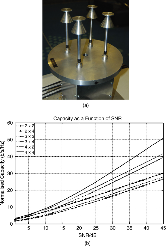
3.17.1 Wideband Channel Model
Similar to the computation of capacity of wideband MIMO channels, the wideband channel model can be expressed in terms of several narrowband channels where now Equation (3.95) represents a single segment of the wideband channel. For example, in [45] the 120 MHz bandwidth was divided into six sections of 20 MHz each, where each frequency section d is characterized by:
3.115 ![]()
References
1. Okumura, Y., Ohmori, E., Kawano, T. and Fukuda, K. (1968) Field strength and its variability in VHF and UHF land mobile radio service. Rev. Electr. Commun. Lab., 16 (9–10), 825–873.
2. Clarke, R.H. (1968) A statistical theory of mobile radio reception. Bell Syst. Tech. J., 47, 957–1000.
3. Aulin, T. (1979) A modified model for the fading signal at a mobile radio channel. IEEE Trans. Veh. Technol., VT-28 (3), 182–203.
4. Parsons, D. (1992) The Mobile Radio Propagation Channel, Halsted Press, John Wiley & Sons Inc., New York.
5. Bennett, W.R. (1948) Distribution of the sum of randomly phased components. Q. Appl. Math., 5, 385–393.
6. Rice, S.O. (1944) Mathematical analysis of random noise. Bell Syst. Tech. J., 23, 292–332.
7. Budden, K.G. (1961) Radio Waves in the Ionosphere, Cambridge University Press, Cambridge.
8. Sollfrey, W. (1965) Effects of propagation on the high frequency electromagnetic radiation from low-altitude nuclear explosions. Proc. IEEE, 53, 2035–2042.
9. Wait, J. (1965) Propagation of pulses in dispersive media. Radio Sci., J. Res. NBS, 69D, 1387–1401.
10. Epstein, M.R. (1968) Polarization of ionospherically propagated hf waves with application to radio communication. Radio Sci., 4, 53–67.
11. Inston, H.H. (1969) Dispersion of hf pulses by ionospheric reflection. Proc. IEE, 116, 1789–1793.
12. Lundberg, B. and Lundgren, M. (1992) On the spectral shape of chirp sounder signals. J. Atmos. Terr. Phys., 54, 311–321.
13. Salous, S. (1994) Dispersion of chirp pulses by the ionosphere. J. Atmos. Terr. Phys., 56 (8), 979–994.
14. Bello, P.A. (1963) Characterization of random time-variant linear channels. IEEE Trans. Commun. Syst., 11, 360–393.
15. Khokhar, K. and Salous, S. (2008) Frequency domain simulator for mobile radio channels and for IEEE 802.16 standard using measured channels. IET Commun., 2 (7), 869–877.
16. Zadeh, L.A. (1950) Frequency analysis of variable networks. Proc. IRE, 38 (3), 291–299.
17. Rummler, W.D., Coutts, R.P. and Liniger, M. (1986) Multipath fading channel models for microwave radio. IEEE Commun. Mag., 24 (11), 30–41.
18. Shankar, P.M. (2002) Introduction to Wireless Systems, John Wiley & Sons, Inc., New York.
19. Steele, R. (1992) Mobile Radio Communications, Pentech Press Ltd, London.
20. Braun, W.R. and Dersch, U.A. (1991) A physical mobile radio channel model. IEEE Trans. Veh. Technol., 40 (2), 472–482.
21. Papoulis, A. (1991) Probability, Random Variables, and Stochastic Processes, 3rd edn, McGraw-Hill, New York.
22. Proakis, J.G. (1993) Digital Communications, McGraw-Hill, New York.
23. Parsons, J.D. and Gardinar, J.G. (1989) Mobile Communications Systems, Blackie & Sons, Ltd, Glasgow.
24. Hashemi, H. (1993) The indoor radio propagation channel. Proc. IEEE, 81 (7), 943–968.
25. Hoffman, W.C. (1960) Statistical Methods in Radio Wave Propagation, Pergamon Press.
26. Suzuki, H. (1977) A statistical model for urban radio propagation. IEEE Trans. Commun., COM-25 (7), 673–679.
27. Lee, W.C.Y. (1985) Estimate of local average power of a mobile radio signal. IEEE Trans. Veh. Technol., 34 (1), 22–27.
28. Hansen, F. and Meno, F.I. (1977) Mobile fading: Rayleigh and lognormal superimposed. IEEE Trans. Veh. Technol., 26 (4), 332–335.
29. French, R.C. (1979) The effect of fading and shadowing on channel reuse in mobile radio. IEEE Trans. Veh. Technol., 28 (3), 171–180.
30. Saunder, S. (1999) Antenna and Propagation for Wireless Communication Systems, John Wiley & Sons, Inc..
31. Winters, J. (1987) On the capacity of radio communication systems with diversity in a Rayleigh fading environment. IEEE J. Sel. Areas Commun., SAC-5, 871–878.
32. Foschini, G.J. (1996) Layered space-time architecture for wireless communication in a fading environment when using multi-element antennas. Bell Labs. Tech. J., 1 (2), 41–59.
33. Foschini, G.J. and Gans, M.J. (1998) On limits of wireless communications in a fading environment when using multiple antennas. Wireless Pers. Commun., 6 (3), 311–335.
34. Wolniansky, P.W., Foschini, G.J., Golden, G.D. and Valenzuela, R.A. (1998) V-BLAST: an architecture for realising very high data rates over the rich-scattering wireless channel. Proceedings of the ISSSE'98, Pisa, Italy.
35. Wennstrom, M. Promises of Wireless MIMO Systems, Uppsala University, Sweden, http://www.signal.uu.se/courses/semviewgraphs/mw_011107.ppt.
36. Holter B. (2001) On the Capacity of the MIMO Channel–A Tutorial Introduction (VTC 01), http://www.ilab).ux.his.no/norsig/finalpapers/57.capacity_of_1992001154555.pdf.
37. Gesbert, D., Bolcskei, H., Gore, D. and Paulraj, A. (2000) MIMO wireless channels: capacity and performance prediction. IEEE Globecom 2000, San Fransisco, CA, Vol. 2, pp. 1083–1088, http://heim.ifi.uio.no/~gesbert/papers/globecom00.pdf.
38. Chishik, D., Rashid-Farroki, F., Ling, J. and Lozano, A. (2000) Effect of antenna separation on the capacity of BLAST in correlated channels. IEEE Commun. Lett., 4 (11), 337–339.
39. Loyka, S. and Kouki, A. (2002) New compound upper bound on MIMO channel capacity. IEEE Commun. Lett., 6 (3), 96–98.
40. Loyka, S. (2001) Channel capacity of MIMO architecture using the exponential correlation matrix. IEEE Commun. Lett., 5 (9), 369–371.
41. Loyka, S. and Mosig, J. (2000) Channel capacity of n-antenna. BLAST Archit. Electron. Lett., 36 (7), 660–661.
42. Chizhik, D., Ling, J., Wolniansky, P. et al. (2003) Multiple input multiple output measurements and modeling in Manhattan. IEEE J. Sel. Areas Commun., 21 (3), 291–292(MIMO Systems and Applications: Part I).
43. Bengtsson, K., Yu, M., Ottersten, B. et al. (2001) Measurement analysis of NLOS indoor MIMO channels. Proceedings IST Mobile Communications Summit, pp. 277–282.
44. Yu, M., Bengtsson, K., Ottersten, B. et al. (2001) Second order statistics of NLOS indoor MIMO channels based on 5.2 GHz measurements. Proceedings IEEE Global Telecommunications Conference, Vol. 1, pp. 156–160.
45. Shiu, D.S., Foschini, G.J., Gans, M.J. and Kahn, J.M. (2000) Fading correlation and its effect on the capacity of multi-element antenna systems. IEEE Trans. Commun., 48 (3), 502–513.
46. Kermoal, J.P., Schumacher, L., Pedersen, K.I. et al. (2000) A stochastic MIMO radio channel model with experimental validation. IEEE J. Sel. Areas Commun., 20 (6), 1211–1226.
47. Zcelik, H.O., Herdin, M., Weichselberger, W. et al. (2003) Deficiencies of the Kronecker MIMO radio channel model. Electron. Lett., 39 (16), 1209–1210.
48. Yu, K. and Ottersten, B. (2002) Models for MIMO propagation channels, a review. Wiley J. Wireless Commun. Mobile Comput. Special issue on Adaptive Antennas and MIMO Systems. doi:10.1002/wcm, 78IR-S3_SB-0223.
49. Gesbert, D., Bolcskei, H., Gore, D. and Paulraj, A. (2002) Outdoor MIMO wireless channels: models and performance prediction. IEEE Trans. Commun., 50 (12), 1926–1934. doi:10.1109/TCOMM.2002.806555.
50. Correia, L.M. (2001) Wireless Flexible Personalised Communications, Chapter 3, John Wiley & Sons, Inc., pp. 77–277.
51. Thomä, R.S., Hampicke, D., Richter, A. et al. (2001) MIMO vector channel sounder measurement for smart antenna system evaluation. Eur. Trans. Telecommun., 12, 427–438.
52. Loyka, S. and Tsoulos, G. (2002) Estimating MIMO system performance using the correlation matrix approach. IEEE Commun. Lett., 6 (1), 19–21.
53. Razavi-Ghods, N. and Salous, S. (2009) Wideband MIMO channel characterization in TV studios and inside buildings in the 2.2–2.5 GHz frequency band. Radio Sci., 44, RS5015. doi:10.1029/2008RS004095.
54. Svantesson, T. and Ranheim, A. (2001) Mutual coupling effects on the capacity of multi-element antenna systems. IEEE ICASSP 01, Salt Lake City, Utah.
55. Gunashekar, S.D., Warrington, E.M., Salous, S. et al. (2009) Investigations into the feasibility of multiple input multiple output techniques within the HF band: preliminary results. Radio Sci., 44, RS0A19. doi:10.1029/2008RS004075.
56. Driessen, P.F. and Foschini, G.J. (1999) On the capacity formula for multiple input–multiple output wireless channels: a geometric interpretation. IEEE Trans. Commun., 47 (2), 173–176.
57. Tarhuni, N. and Korhonen, T.O. (2002) Influence of environment on capacity of LOS city street MIMO channel. URSI/IEEE XXVII Convention on Radio Science, pp. 126–128.
58. Burr, A. (2000) Channel Capacity Evaluation of Multi-Element Antenna Systems Using Spatial Channel Model AP2000, Davos, Paper 231.
59. Burr, A.G. (2002) Capacity of MIMO systems in realistic cellular wireless systems. IEE Conference Publication 02/112, ‘Getting the Most Out of the Radio Spectrum’, 24–25, pp. 26/1–26/5.
60. Gunashekar, S.D., Warrington, E.M., Feeney, S.M. et al. (2010) MIMO communications within the HF band using compact antenna arrays. Radio Sci., 45, RS6013. doi:10.1029/2010RS004416.
61. Loyka, S. and Kouki, A. (2002) On MIMO channel capacity, correlations and keyholes: analysis of degenerate channels. IEEE Trans. Commun., 50 (12), 1886–1888.
62. Chizhik, D., Foschini, G., Gans, M. and Valenzuela, R. (2002) Keyholes, correlations and capacities of multi-element transmit and receive antennas. IEEE Trans. Wireless Commun., 1 (2), 361–367.
63. Ling, J., Chizhik, D. and Valenzuela, R. (2001) Predicting multi element receive and transmit array capacity outdoors with ray tracing. IEEE Veh. Technol. Conf., 1, 392–394.
64. Ecreg, V., Soma, P., Baum, D.S. and Paulraj, A.J. Capacity Obtained from Multiple Input Multiple Output Channel Measurements in Fixed Wireless Environments at 2.5 GHz, www.nari.ee.ethz.ch/commth/pubs/viewpub.php?ident=ESBP02.
65. Yu, K., Bengtsson, D.M., Ottersten, B. and Beach, M. (2002) Narrowband MIMO channel modelling for LOS indoor scenarios. URSI 27th General Assembly, Maastricht, 17–24 August 2001, 2002, Paper 0162.
66. Paulraj, A., Nabar, R. and Gore, D. (2003) Introduction to Space-Time Wireless Communications, Cambridge University Press.
67. Jenson, M.A. and Wallace, J.W. (2004) A review of antennas and propagation for MIMO wireless communications. IEEE Trans. Antennas Propag., 52 (11), 2810–2824.