Chapter 4
Radio Channel Sounders
In this chapter we review the history of radar and show the similarity between radars and sounders. We then discuss the different modes of operations and suitable waveforms including continuous wave, narrow pulse and pulse compression waveforms. We then outline architectures suitable to implement single input–single output to multiple input–multiple output sounders for different applications. We investigate the range Doppler ambiguity that might arise in certain applications and present advanced waveforms that can resolve this ambiguity. Finally, we discuss typical calibration procedures.
4.1 Echoes of Sound and Radio
The use of the word ‘sounder’ for determining distance goes back to the early seventeenth century where sounding was used to determine the depth of water in rivers and lakes by means of a line and plummet. Early usage of sounders was mainly for the determination of any physical property at a depth in the sea or at a height in the atmosphere, such as the temperature soundings made in 1875.
After the disaster of the Titanic in 1912, the German physicist Alexander Behm conducted research to find a way to detect icebergs. He discovered echo sounding, which he patented in 1913. However, echo sounding turned out to be inefficient in spotting icebergs, but a great tool to measure the depth of the sea. Thus echo sounding is defined as the technique of using sound pulses directed from the surface or from a submarine vertically down to measure the distance to the bottom of the sea. This has been adopted as the main technique since about the middle of the 1920s. In addition to navigation, echo sounding was used to aid fishery. Distance was related to the speed of sound in water either by taking an average speed of sound of about 1.5 km/s or, for more accurate scientific surveys, a sensor is used to measure the water temperature, salinity and pressure to estimate the local speed of sound. High resolution maps of sea beds and oceans were determined by autonomous underwater vehicles (AUVs) equipped with a multibeam echo sounder (MBES), which uses around a hundred transducers to transmit and listen to the echoes. The output of the transducers is combined using beam forming to determine the direction of the echo.
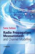
In contrast to echo sounding, radio sounding, also widely used in Oceanography, Meteorology and Geology, uses echoes of electromagnetic waves. The existence of electromagnetic waves was predicted by the Scottish physicist James Clerk Maxwell (1864), but it was the German physicist Heinrich Hertz who first succeeded in generating and detecting radio waves in 1886. Hertz used a spark gap less than 0.3 mm to generate the excitation and an optical magnifying lens system to detect it. Hertz's experiments also showed that radio waves could be reflected by metallic and dielectric objects. The device that could detect an alternating electrical signal across its terminals was invented by Edouard Branly in 1890, which in 1894 was called the ‘coherer’ by Oliver Lodge. In 1895 Marconi linked electromagnetic (EM) waves to wireless communications, and this sparked a great deal of interest among scientists and fortune hunters. In 1904 Christian Hülsmeyer (Figure 4.1a) demonstrated in Germany and in the Netherlands the use of radio echoes to detect ships up to a range of 3 km, using a simple spark gap directed with a multipole antenna. The invention was patented and the device was called the telemobiloskop (Figure 4.1b) which stands for tele: far off or covering a distance, mobil: capable of moving or being moved, skop: scope area covered by an activity. The telemobiloskop did not provide range information, but only warning of a nearby object to avoid collisions. Later in 1904, Hülsmeyer patented an amendment for ranging that uses a vertical scan in conjunction with the telemobiloskop mounted on a tower [1] to identify the most intense return and to deduce, by simple triangulation, the approximate distance. Hülsmeyer's invention covered all the basic concepts of radar: (i) reflection of EM waves off a conducting object with a split transmitter and receiver, (ii) 360o, synchronous, area coverage of targets later called a plan position indicator (PPI) radar, (iii) measuring the distance to the target, (iv) platform for stabilizing the system and (v) implementation of a protection for the system from the environment (nowadays called radome).
Figure 4.1 Photographs of (a) Christian Hülsmeyer and (b) Telemobiloskop [1].
Source: Radar World, http://www.radarworld.org/. Reproduced with permission.
In 1917 Nicola Tesla stated the principles of radar using standing electromagnetic waves along with pulsed reflected surface waves to determine the relative position, speed and course of a moving object.
Hülsmeyer's experiments were ahead of the technology at the time as he used a relatively short wavelength (66 cm) and his apparatus was dismissed. On 20 June of the year 1922 Marconi urged the use of short waves for long range detection of ships, as delivered in a speech he gave at a joint meeting of the Institute of Radio Engineers and the American Institute of Electrical Engineers in New York, in which he said:
As was first shown by Hertz, electric waves can be completely reflected by conducting bodies. In some of my tests I have noticed the effects of reflection and detection of these waves by metallic objects miles away.
It seems to me that it should be possible to design apparatus by means of which a ship could radiate or project a divergent beam of these rays in any desired direction, which rays, if coming across a metallic object, such as another steamer or ship, would be reflected back to a receiver screened from the local transmitter on the sending ship, and thereby, immediately reveal the presence and bearing of the other ship in fog or thick weather.
Marconi's suggestion seems to have inspired A.H. Taylor and L.C. Young of the Naval Research Laboratory who used a continuous waveform (CW) interference radar with 5 m wavelength, with separate transmitter and receiver, to detect a wooden ship in the autumn of 1922. The first application of the pulse technique for the measurement of distance was by Breit and Tuve in 1925, in a sounding application for measuring the height of the ionosphere.
Since the 1920s radar and sounders were applied in many areas such as astronomy, meteorology, aurora, meteors and microwave spectroscopy. Examples of reported applications include the radio sounding device used to register the depths of the ocean (1922, The Marine Journal), radio sounding balloons released from the Graf Zeppelin for weather applications (1929, The Bulletin of the American Meteorological Society) and the detection of dry layers that appear from time to time in the troposphere (1947, Science Progress XXXV). In 1963 The Times speculated that a form of radio sounding, similar to radar, may provide a new means of charting the depth of rock surfaces covered by snow and ice, as in Greenland and Antarctica, and in 1993 The Atmospheric Research stated that atmospheric profiles of temperature and humidity were obtained from radio soundings on cloud-free days.
The principles of operation of a radio sounder and its development are thus closely related to radar systems. The distinction between radars and sounders is best related to the objectives that each system desires to achieve and in the treatment that follows; the differences and similarities between radars and sounders are discussed where appropriate.
4.2 Definitions and Objectives of Radio Sounders and Radar
A RADAR (radio detection and ranging) is defined as a system that detects the electromagnetic wave reflected off a target to determine one or more of its following parameters: (i) range, which is determined by measuring the time taken for the radar signal to travel to and back from the target, (ii) radial velocity, which is determined by measuring the relative shift in the carrier frequency of the reflected wave (Doppler effect), and (iii) angular position, which is determined from the direction of arrival (DOA) of the wavefront, using a number of techniques including directional antenna beams or antenna arrays with classical and modern signal processing techniques.
A channel sounder, on the other hand, is a system that detects the electromagnetic wave transmitted via a particular communication channel to determine the statistics of either the channel's time-variant impulse response or its time-variant frequency response. The echoes are usually referred to as multipath components and their extent in time delay is used to aid in the design of wireless communication systems. In addition to the time delay and the relative strength of the echoes a channel sounder may aim to estimate Doppler shift or Doppler spread. Modern channel sounders deploy a number of techniques similar to radar to estimate angular information, including angle of departure and angle of arrival in azimuth and in elevation. This gives rise to a variety of channel sounder configuration, including single and multiple antennas at both ends of the radio link which can be employed in different modes of operation.
4.2.1 Modes of Operation
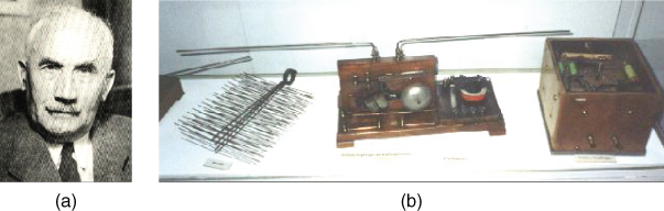
Both radars and sounders can be deployed in a static or dynamic mode of operation. Static operation refers to the situation where both the transmitter and the receiver are stationary whereas dynamic operation refers to the situation when one or both terminals are in motion. In either case the target, environment or reflectors can be stationary or in motion. A static system that uses the same antenna for transmission and reception is termed monostatic, as illustrated in Figure 4.2a, whereas a system that deploys separate antennas or has a separate site for transmission and reception is termed bistatic as shown in Figure 4.2b. In Figure 4.2, if either terminal(s) are in motion, the mode of operation becomes dynamic. Depending on the number of antenna elements used for transmission or reception the prefix ‘multi’ can also be used to indicate multiple antennas such as multistatic, where the same set of antennas are used for transmission and reception. For example, a monostatic sounder pointing vertically upwards is usually deployed for ionospheric studies to determine the height of the reflecting layers, while a monostatic radar is the general form of radar used in collision avoidance and radiometers. Long range skywave communication studies and mobile radio propagation require separate transmit and receive terminals. Multiple antenna radars are used in sea state studies with single-site or dual-site transmission and reception.
Figure 4.2 Configuration of radar and sounder systems: (a) monostatic and (b) bistatic.
4.2.2 Basic Parameters
A radar or sounder aim to estimate a number of parameters, which can include the following:
Depending on the parameters of interest a number of waveforms and architectures can be deployed in radio channel sounding or radar applications. In the following section we will study some of these waveforms and the parameters that can be estimated from each waveform.
4.3 Waveforms
Essential to the design of a radar or sounder system is the appropriate choice of the transmitted waveform, which determines the parameters that can be estimated. Factors considered in the choice of the waveform include: detection, resolution, ambiguity and measurement accuracy.
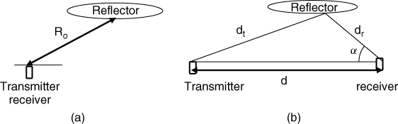
In the following analysis the waveforms will be classified as illustrated in Figure 4.3.
Figure 4.3 Classification of waveforms used in radar or sounder applications.
4.4 Single-Tone CW Waveforms
The single-tone system has many advantages, which include:
Conversely, a CW system cannot detect range in a radar application and nor can it estimate the time delay in a sounder application. Limited multipath resolution can be achieved via Doppler analysis, and a very serious problem is the direct leakage from the transmitter to the receiver (spillover) in a single site (monostatic) configuration. In addition, the frequency coherence function cannot be obtained.
The main popular applications of CW systems include police radars, speedometers, CW proximity fuses and measurement of the attenuation (path loss) and fading statistics over a radio link.
4.4.1 Analysis of a Single-Tone System
A CW system transmits a continuous wave signal ST(t) at an angular frequency, ωc = 2πfc rad/s and receives a signal SR(t), which consists of N echoes as given by:
where An(t), τn, are the amplitude and the time delay of the nth echo or multipath component respectively.
The time delay usually consists of two contributions, one corresponding to the distance travelled between the transmitter to a stationary receiver, Ro, and the other due to the relative velocity of the echo vr. This can be deduced from the fact that the time of travel between the transmitter and a stationary receiver in both of Figure 4.4a,b is equal to τo and is related to Ro, where in the bistatic configuration it corresponds to the sum of the distance from the transmitter to the reflector and from the reflector to the receiver, while in the monostatic case it is simply the distance to the reflector. If this distance is increased or decreased, an additional time delay component δτd related to the speed of travel of the reflector or receiver needs to be included to account for this change.
Figure 4.4 Change in the range between the transmitter and the receiver due to (a) the movement of the receiver in a bidynamic system and (b) the movement of the reflector in a monostatic system.
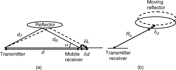
Considering first Figure 4.4a, where the receiver is at distance d from the transmitter, the time of travel is then:
where cp is the speed of travel of the wave in the medium and for propagation in the atmosphere is close to the free space speed of light c, which is equal to 2.998 × 10⁸ m/s.
In the case of Figure 4.4b, Equation (4.2) becomes:
Substituting Equation (4.3) into Equations (4.1a) as an example and assuming free space propagation we obtain, for the single-target case:
4.4 ![]()
Noting that for a CW signal a rotation in the phase in excess of 2π radians cannot be measured without ambiguity, the maximum range that can be estimated for any echo as measured from the phase difference Δφ between the transmit and receive CW tone is given by:
or, equivalently,
4.5b ![]()
Similarly, any phase difference that is equal to 2πk + δφ, where k is an integer, is indistinguishable from δφ and is therefore ambiguous.
While CW radars or sounders have no capability in detecting range, they can be used to estimate Doppler shift, which arises from the movement of either the transmitter or receiver or the movement of the reflector. Referring to Figure 4.4 and considering a single reflector, the distance travelled by the receiver or reflector ![]() is given by:
is given by:
4.6 ![]()
where ![]() is the speed of travel of the receiver or reflector and
is the speed of travel of the receiver or reflector and ![]() is the difference in the time of travel.
is the difference in the time of travel.
This gives rise to an increase in the propagation path length from the reflector to the receiver, ![]() as given in Equation (4.7a) for Figure 4.4a and Equation (4.7b) for Figure 4.4b, assuming radial movement of the target:
as given in Equation (4.7a) for Figure 4.4a and Equation (4.7b) for Figure 4.4b, assuming radial movement of the target:
This difference in range translates to a phase change Δφ as in Equations (4.8a) whose derivative with respect to time gives an apparent change in frequency fd, where the positive and negative signs represent a reflector that is approaching or receding respectively. The resulting relationships of the phase and corresponding Doppler shifts for Figure 4.4a are given in Equations (4.8a) and (4.8b), while the corresponding relationships for Figure 4.4b are given in Equations (4.8c) and (4.8d):
where λ is the wavelength of the carrier.
Taking the Doppler shift into account and the time delay due to the range of the reflectors, Equation (4.1b) becomes:
where ![]() is the phase shift due to range and
is the phase shift due to range and ![]() is the Doppler shift of the nth reflector. Equation (4.9) is similar to the previously derived Equation (3.3.5) for the scattering model. However, in Equations (4.7–4.8), the Doppler shift is only related to the azimuth angle
is the Doppler shift of the nth reflector. Equation (4.9) is similar to the previously derived Equation (3.3.5) for the scattering model. However, in Equations (4.7–4.8), the Doppler shift is only related to the azimuth angle ![]() whereas Equation (3.3.4.1) gives the more generalized relationship.
whereas Equation (3.3.4.1) gives the more generalized relationship.
When the velocity is not constant, the Doppler frequency shift varies with time and results in a spread of the frequency over a range related to the acceleration ar and the duration of observation interval ΔT by ±2arnΔT/λ.
Another case of interest is when both the transmitter and the receiver are in motion, such as in vehicle-to-vehicle communication. The resultant change in range and hence in Doppler shift is a function of their relative speed and depends on whether they are moving in the same direction or in opposite directions, as shown in Figure 4.5.
Figure 4.5 Vehicle-to-vehicle communication: (a) two vehicles travelling in the same direction and (b) vehicles travelling in opposite directions.
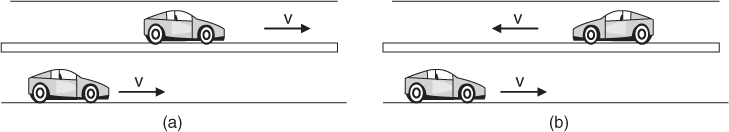
If the two vehicles are moving in the same direction as in Figure 4.5a and at the same speed then the apparent change in phase is zero, while if they are travelling in opposite directions the distance between them is changing with time, first decreasing until they cross over and then increasing as they move farther away from each other. This results in an initial positive Doppler shift, which changes to a negative Doppler shift. The maximum shift in frequency is now given by:
4.10 ![]()
While a CW sounder or radar has no range resolution, if the multipath components or echoes have different Doppler shifts, which might arise due to differences in the angle of arrival or in speed, then the echoes can be resolved from Doppler analysis of the received signal. Estimation of the Doppler shift can be obtained by mixing the incoming signal with a coherent local oscillator (LO) either at the same frequency as the transmitted carrier or with an offset frequency to generate an IF. Consider first the case when the IF is set to zero; the received signal in Equation (4.9) becomes:
4.11 ![]()
Different targets can be discriminated if they have different Doppler frequencies, but the sign of the Doppler shift is lost in this case due to the folding of the negative and positive frequencies. Using an IF on the other hand allows the detection of frequencies above and below the IF and hence the sign of the Doppler shift is preserved, as expressed by:
Passing the signal in Equation (4.12) through a bank of analogue filters enables separation of the different targets or multipath components. Alternatively, using a data logger, the digitized signal can be analyzed using the fast Fourier transform (FFT). The FFT gives a sin x/x function, which has high sidelobe levels and a time delay resolution that is inversely proportional to ΔT, which is the acquisition time or the duration of the signal used in the spectrum analysis. These effects can be reduced via windowing as discussed in Section 5.2. While in theory increasing the acquisition time should increase the Doppler resolution, a limit is reached as set by the phase noise of the LOs. Phase noise broadens the peak of a CW signal and is a function of the spectral purity of the oscillators.
The Doppler frequency shift of a reflector moving at a nonconstant speed also gives rise to an offset in Doppler frequency equal to Δfd = ±2ariΔT/λ, which can spread the Doppler frequency over a number of frequency bins where each bin is equal to 1/ΔT. To contain each return in the width of the bin or filter, the largest value of ΔT should be equal to 1/Δfd, which results in a Doppler spread equal to:
4.13 ![]()
An alternative to using an IF is to mix the received signal down to baseband using quadrature demodulation to obtain the baseband in-phase and quadrature components. Expanding Equation (4.9) as in Equation (3.3.5), the received signal can be expressed as:
4.14 
When mixed with coherent LOs with ![]() and
and ![]() , and filtered to remove the high frequency (HF) components, the received signal can be expressed as:
, and filtered to remove the high frequency (HF) components, the received signal can be expressed as:
The in-phase and quadrature components in Equation (4.15) can be combined to estimate the received signal strength and the phase, as illustrated in the phasor diagram of Figure 4.6, given as:
Figure 4.6 Phasor diagram representation of the received signal.
Complex spectral analysis of Equation (4.16) resolves the multipath components according to their Doppler shift, where the sign indicates whether the echo is receding or approaching. Evaluating the envelope ![]() and the phase
and the phase ![]() for each resolved component gives its corresponding magnitude and phase, and the frequency at which the component is resolved gives the Doppler shift.
for each resolved component gives its corresponding magnitude and phase, and the frequency at which the component is resolved gives the Doppler shift.
Equation (4.15) is based on the assumption that the generators at the receiver have 90° phase shift. An imbalance between the two carrier components and phase drift can cause a spillage between the two baseband components, which can be avoided by mixing down to a low IF.
4.5 Single-Tone Measurements
4.5.1 Measurement Configurations
A CW sounder is capable of estimating two main parameters: signal strength variations at a particular carrier frequency, both small-scale fading and large-scale (path loss), and Doppler shift or Doppler spread. The architecture of a CW sounder therefore depends on which parameter is to be estimated.
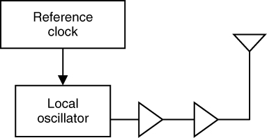
Generally a CW sounder consists of a signal generator or an LO at the transmitter, which can be based on phase locked loop (PLL) techniques at the required carrier frequency, the necessary amplification to a power level to cover the maximum range of interest and a calibrated antenna. To avoid frequency drift, the LO is locked to a high stability reference, which is derived from a crystal or a rubidium clock as shown in Figure 4.7.
Figure 4.7 Transmitter configuration for CW measurements.
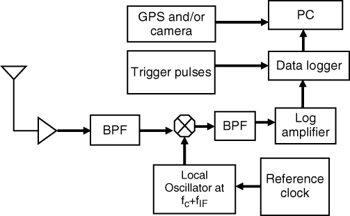
At the receiver, a calibrated antenna followed by low noise amplification and a bandpass filter form the RF front end where the architecture of the rest of the receiver depends on the required parameters. As discussed in Section 4.2, there are two basic architectures that can be deployed at the receiver. A heterodyne detector followed by envelope detection gives the signal strength variations whereas a quadrature detector gives both signal strength variations and phase information. Signal strength variations can thus be obtained using either off the shelf equipment such as a spectrum analyzer as in Figure 4.8 or a custom designed receiver as shown in Figure 4.9.
Figure 4.8 Signal strength measurement receiver based on a spectrum analyzer.
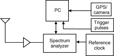
Figure 4.9 Heterodyne receiver architecture for measuring the received signal strength.
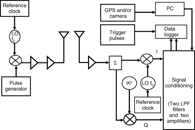
In Figure 4.8, the spectrum analyzer provides a simple receiver where a preamplifier boosts the received signal strength to increase the dynamic range of the measurement. The received signal is then logged to a computer via the analyzer's PC interface and the data logging can be synchronized with trigger pulses. In these measurements the trigger pulses are derived either from a wheel sensor configuration (see Section 4.5.2) or from a predetermined distance displacement trigger such as an xy positioner or turntable, which relate the signal strength variation to the distance travelled or positions (spatial sampling) or are derived from a timing clock such as from a global positioning system (GPS) to give the time variability of the environment (time sampling). The latter is useful for static transmitter and receiver configurations. Additional environmental observations can be added during data logging, which can include information from a GPS receiver to provide geographic location information as well as a time stamp and video camera or voice commentary logging to relate the data to the local environment. The spectrum analyzer can be configured for a narrow resolution bandwidth and a small frequency sweep. For example, a spectrum analyzer configured for a 3 kHz resolution bandwidth with a 2 kHz frequency sweep can provide 601 points for each one second sweep. The measurements can then be averaged to remove noise effects and/or to average out fast fading during the estimation of path loss. Issues to be considered in this regard are the acquisition time between files, which can be lengthy due to the data transfer rate via the PC interface. The spectrum analyzer can also be configured for multiple frequency band measurements where the parameters for each band are programmed via a separate menu, such as setting the start and end frequencies, the sweep time and the filter bandwidth. The spectrum analyzer can be phase locked to the transmitter by using a reference oscillator at both ends of the link to ensure that the signal remains within the observation window of the analyzer during measurements.
Figure 4.9 gives an alternative receiver to the spectrum analyzer where the incoming CW signal is amplified, bandpass filtered and mixed with an LO offset from the transmitted carrier by an intermediate frequency fIF, usually around 70 MHz, which can be filtered and amplified using a log amplifier. The log amplifier produces a DC voltage proportional to the logarithm of the input power and hence enhances the dynamic range of the receiver. The data can be logged in when triggered. The bandwidth of the bandpass filters (BPFs) in the receiver should be chosen to accommodate the highest expected Doppler frequency to ensure appropriate detection of the signal.
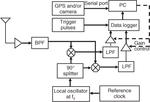
Figure 4.10 displays a suitable architecture for a quadrature receiver that can be used to obtain both the envelope and the phase. Similar to the configuration of Figure 4.9, the bandwidth of the lowpass filter (LPF) should be chosen to accommodate the highest expected Doppler frequency and the amplifiers in the signal conditioning (SC) provide adequate gain to generate a suitable signal for the analogue to digital converter (ADC) in the data logger. This can be accomplished by adjusting the gain via a feedback mechanism from the PC.
Figure 4.10 Quadrature receiver architecture.
Path loss measurements are generally performed with omnidirectional antennas. When directional antennas are used to reduce the required amplifier gain, at each location of measurement the receive antenna needs to be aligned to point to the transmitter and vice versa. This can be achieved by roughly aligning the antennas by reference to maps of the area and compass bearings. The antennas can then be adjusted to maximize the received signal strength. To evaluate the path loss accurately, all equipment used should be calibrated, including measuring the gain and radiation pattern of the antennas, losses in the cables to and from the antennas, gains of all amplifiers and the sensitivity of the receiver. All of these parameters need to be compensated for in the calculation of the path loss.
4.5.2 Triggering of Data Acquisition
Triggering of data acquisition can be set up either for spatial sampling or for time sampling. In either case, measurement of the Doppler shift requires sampling at the Nyquist rate, which is at least twice the maximum Doppler shift. However, to study the signal strength variations to identify deep fades it is necessary to sample at a much higher rate, which depends on the fade depth to be estimated. For example, for a Rayleigh fading signal, in order to detect about 50 % of fades 30 dB below the median level, the signal must be sampled every 0.01λ [2]. For most practical purposes a sample every λ/3 can be sufficient [3] to determine the statistical distribution of the fading envelope. In the following we first discuss spatial sampling modes of operation followed by time sampling:
4.17 ![]()
Figure 4.11 (a) Wheel sensor configuration [4] and (b) toothed wheel mounted on the fifth wheel.
Source: Abdalla, M. M., (2005) Directional antenna array for channel measurement system. PhD thesis University of Manchester Institute of Science and Technology. Reproduced with permission.
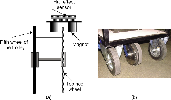
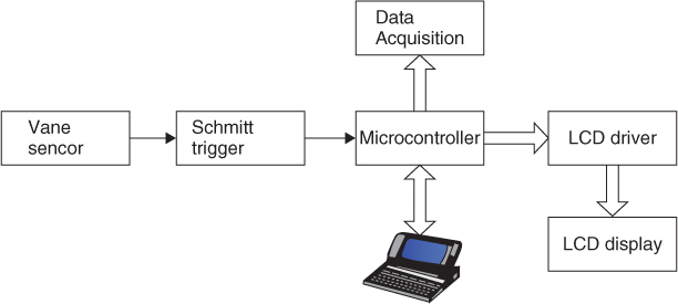
The pulses from the sensor are usually sharpened by using a Schmitt trigger prior to connecting to the data acquisition circuit. The wheel sensor pulses can be used either directly to provide the clock for the acquisition of data, thus ensuring that the samples are separated by the same spatial distance, or can be counted by a microcontroller over a specified time interval and using a separate clock for the acquisition of data. In this case the wheel sensor pulses give the overall distance travelled, which can be used to provide an average distance between samples. This approach is useful if averaging of consecutive data samples is employed to reduce the effect of additive noise. Figure 4.12 displays a possible configuration for a wheel sensor circuit, where the microcontroller can be reset at the required time interval and the distance travelled can be logged in or displayed [4].
Figure 4.12 Block diagram of wheel sensor circuit for estimation of travel distance [4].
Source: Abdalla, M. M., (2005) Directional antenna array for channel measurement system. PhD thesis University of Manchester Institute of Science and Technology. Reproduced with permission.
For a single wheel sensor distances are measured relative to one direction heading. If the trolley or car is not moving in a straight direction then a dual sensor arrangement would be needed to measure the x–y displacement.
Constant speed can be also enabled through motors controlling the wheels of the trolley or using automatic cruise in a car.
- Static mode. For controlled environments such as indoor measurements or a parked trolley or van a track can be set up to trigger the data acquisition with a controller that moves the antenna by precise displacements. Small-scale fading is then averaged out by either rotating the antenna element by a number of prescribed steps in azimuth or moving the antenna over a linear track mounted on the vehicle. The measurements are then repeated for a number of locations to obtain path loss estimates as a function of distance [5, 6].
- Time sampling. For static operation, time sampling can be used where the acquisition of data is triggered by a clock derived from a time reference, which is related to the time variability of the channel, that is the maximum Doppler shift. In the static mode the only variations observed are due to the movement of people during working hours in an office environment [7] or vehicles in city centres and motorways with high traffic mobility. These movements can result in significant time variability manifested as time fading.
4.5.3 Strategy of CW Measurements
Measurements of path loss require the choice of the transmitter location, the type of antennas to be used and their height above ground, the maximum range to be surveyed, the environment and the application. Measurements can be performed for fixed radio links such as for repeater links, base station to base station, campus or neighbourhood area to stationary users as well as for mobile radio links in indoor or outdoor environments. Measurements can be performed over short or long ranges depending on the application.
Measurements of path loss over fixed radio links require observation of the time variability of a radio channel, either over a short period of time or over long periods. Propagation via a natural medium such as the troposphere or the ionosphere where the propagation mechanism is affected by the solar cycle requires static measurements. Similarly, propagation into forests or over sea paths where the weather conditions affect the path loss can also be considered static. Such measurements are usually taken over a prolonged period of time, which can extend to several years, and the data are analyzed for diurnal and seasonal variations. In the example of propagation over three sea paths in the British Channel Islands, at 2 GHz, signal strength measurements were collected over a two year period [8] during two 1 second intervals in each minute, giving 2880 data points per day per antenna. Another example of long term path loss measurements for microwave links have been set up in the UK at 1.7 GHz, 7.5 GHz and 18.6 GHz and the geometry of the paths was chosen to cover different path orientations and to monitor interference between links that extended from 60 km to 80 km. In the study a sample every 1 second was taken over two years [9]. In other studies such as ionospheric propagation measurements can extend over an 11 year period to cover a whole solar cycle. As with any such path loss measurements it is important to choose the sites properly to extract the relevant information. For example, in ionospheric propagation, the length of the radio link and the orientation of the propagation path with respect to the earth's magnetic field, are among the considerations to setting up the radio link for path loss measurements.
Indoor mobile radio measurements and short range outdoor measurements can be performed using a trolley with a wheel sensor, whereas outdoor macrocellular measurements can extend up to several kilometres and require the use of a van fitted with a mast and distance trigger. Thus, as with sampling, the measurement strategy has to identify static versus dynamic measurements. Indoor measurements of path loss can be performed in a single room, in corridors, office environment factory environments and between floors. These require the mounting of antennas at either ceiling height or on the wall for transmission, or at desk height or an average person's height for reception.
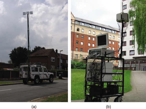
Dynamic measurements, on the other hand, require the movement of either terminal or both terminals as in vehicle-to-vehicle communication. For example, path loss measurements between a fixed terminal and a mobile terminal require the mounting of the transmit antenna on top of a high building or a lamp-post at about 8–200 m above ground and a mobile terminal where the receiver's antenna is at 1 and 9 m. This is usually mounted on top of a vehicle or in a van with a pump-up mast between. The height of the transmitting and receiving antennas depends on the application. For macrocells where the range of coverage extends to several kilometres, the transmit antenna is usually mounted on top of a building at about 46 m, as in the measurements of Ibrahim and Parsons [10], or at 200 m, as in the measurements of Okumura et al. [11]. To account for different antenna heights Okumura gave different sets of equations and correction factors were introduced. For microcellular applications where the range is within 1 km, it is usual to mount the antennas at lamp-post height below the rooftop of buildings and the receive antenna can be between 1.7 m and 2 m. Communication to pedestrians can be evaluated using a trolley, which can be pushed along the pavement, whereas vehicular communication can be studied by using a van or a car as illustrated in Figure 4.13.
Figure 4.13 (a) Measurement set-up using a van with a pump-up mast and (b) receiver mounted on a trolley for pedestrian measurements.
4.6 Spaced Tone Waveform
In a single-tone CW system, comparing the phase of the transmitted signal with the received signal can give range information of a single target if it is limited to 2π radians as expressed in Equation (4.5). Since radars and sounders operate at high frequencies, the wavelength is usually small and hence the range that can be measured with a CW system is insignificant.
To estimate range to a target a time reference is required, which can be achieved by a narrow pulse. An alternative simple solution to overcome the limitation of the single CW tone of range estimation is to transmit simultaneously or sequentially a two-tone waveform consisting of two frequencies separated by Δf. The received signal from the two tones due to a single stationary target is now expressed as:
4.18 ![]()
Applying the relationship in Equation (4.5a) to each of the two tones gives ![]() and
and ![]() . Taking the difference in phase between the two tones now gives:
. Taking the difference in phase between the two tones now gives:
where
![]()
Substituting for the phase difference by 2π in Equation (4.19) gives the maximum unambiguous range that can be measured for a single target as:
Equation (4.20) shows that the maximum unambiguous range that can be measured is inversely proportional to Δf. If Δf is small, then the Doppler frequency shift effects on Equation (4.20) can be assumed to be negligible and the range of the target can be found by taking the phase difference ![]() between the coherently demodulated signals at the two frequencies. However, the minimum frequency difference that can be transmitted is imposed by the maximum expected Doppler shift. As each carrier experiences a Doppler shift due to the movement of the target, the two received frequencies can become indistinguishable if the frequency shift is large enough such that fd > Δf/2.
between the coherently demodulated signals at the two frequencies. However, the minimum frequency difference that can be transmitted is imposed by the maximum expected Doppler shift. As each carrier experiences a Doppler shift due to the movement of the target, the two received frequencies can become indistinguishable if the frequency shift is large enough such that fd > Δf/2.
Another consideration in the choice of Δf is the maximum range error, δRRMS, which is given by [12]:
4.21 ![]()
where E is the energy in the received signal and No is the power spectral density of noise. Therefore increasing the frequency difference reduces the range error at the expense of the reduction in the maximum unambiguous range. In order to obtain both accurate and unambiguous range measurements, three or more frequencies can be transmitted. For example, in [12] it is proposed that to transmit t f1, f2 and f3, where f3 − f1 = a(f2 − f1), where a is set to 10 or 20. Then an accurate measurement, which is ambiguous in the maximum range, can be obtained by comparing the phases between f1 and f3, whereas comparing the phases between f1 and f2 resolves the ambiguities in the measurements of f3 and f1. This shows that to increase the accuracy we can add more and more frequencies, and therefore essentially increase the bandwidth of the transmitted signal, which becomes closer and closer to a linearly frequency modulated signal.
The two-tone system is only capable of measuring the range of a single target since there is only a single phase difference that can be measured. If more than one target is present, then the received signal after the detector consists of the sum of the phases due to the multipath components, and therefore comparing the phases of the received signals at the two frequencies becomes ambiguous. Multiple targets can be discriminated as in the single-tone method by using a bank of filters or spectral analysis.
Applications of the two-tone radar include the Tellurometer, which is a portable surveying radar capable of measuring line of sight distances from 500 ft to 40 miles. It transmits four single sideband (SSB) signals at 10 MHz, 9.99 MHz, 9.9 MHz and 9 MHz with a 3 MHz carrier [12, p. 110].
In sounding, the received signal at the two tones, which consists of the sum of the multipath components, can be correlated to find the frequency coherence at a particular instant in time. For channels whose frequency coherence is a function of frequency, such as the ionosphere, these measurements have to be repeated for that frequency spacing to cover the whole spectrum of interest. Moreover, to obtain the frequency coherence of the channel the required spectrum has to be scanned for different values of Δf. Since the time required to complete the sounding might be longer than the coherent time of the channel, the instantaneous frequency response is not obtained. This can be overcome by simultaneously transmitting a number of frequencies, which are adequately spaced in frequency for a certain time to provide the data necessary to evaluate the frequency and time coherence of the channel. This method has been used both in mobile radio [13] and in narrowband HF [14] to obtain the coherence function.
Figure 4.14 shows a possible configuration for a two-tone transmitter and receiver system where each transmitted tone is mixed with a phase coherent locally generated carrier. The output of each mixer is proportional to the phase difference between the transmitted signal and the local reference. The output of the two mixers can then be applied to a phase detector to estimate the range or logged in and compared digitally. Adding quadrature demodulators at each frequency can give the envelope at each carrier the ability to estimate the path loss and signal strength fading as well as the Doppler frequency, which can be estimated as for the single tone via FFT processing.
Figure 4.14 Block diagram of a two-tone system for measurement of range of a single target.
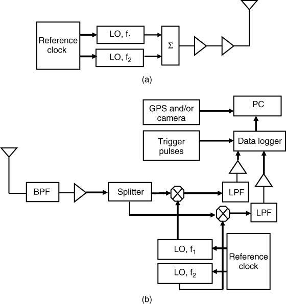
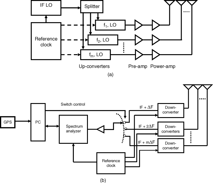
A possible multifrequency system to measure path loss at different frequencies is illustrated in Figure 4.15. At the transmitter the multiple frequency sources are locked to a single IF, which is in turn locked to a reference clock. Similarly, at the receiver, the down-converters bring the multiple frequencies close to the IF LO at the transmitter where a frequency offset is used to separate the multiple frequencies and to avoid spillover from the RF switch. Such a system can be operated with a low frequency spectrum analyzer and avoids the need for high end measurement equipment.
Figure 4.15 Block diagram of a multifrequency measurement set-up using a single spectrum analyzer: (a) transmitter and (b) receiver.
4.7 Pulse Waveform
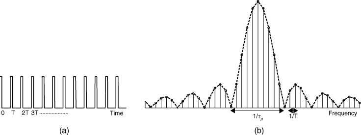
As discussed in Section 4.6 on the spaced tone method, range information of multiple targets requires the transmission of a number of frequencies, which occupy a specified bandwidth. The larger the number of frequency components, the larger is the number of echoes that can be detected in range. Conversely, using Fourier transform properties a periodic signal that has a number of discrete frequency components can be used, such as a periodic pulse train, as illustrated in Figure 4.16.
Figure 4.16 Pulse train: (a) in time domain and (b) in frequency domain.
In sounding applications, a pulse sounder measures the impulse response of the channel. If the pulse time width is adequate to resolve the multipath components, then the received signal strength as a function of time delay gives a snapshot look at the multipath structure. Repetitive pulse sounding represents a ‘motion picture’ of the multipath propagation between the transmitter and the receiver.
4.7.1 Properties of the Pulse Waveform
Recall from Section 4.3 that in a radar or sounder application, resolution and ambiguity are two criteria that need to be considered in the choice of the waveform. Thus for a pulse waveform we would need to relate the following parameters to the transmitted waveform:
4.7.1.1 Time Delay Resolution
Viewed on the time axis range information requires a time reference, which can be obtained from transmitting a narrow pulse of width τp seconds every T seconds as shown in Figure 4.17. In a monostatic application, the time displacement of the received pulse with respect to the transmitted pulse τi gives the range information, while in a bistatic application a synchronized pulse train would be needed at the receiver.
Figure 4.17 Periodic pulse train for range detection: solid line, transmitted pulses and dashed line, received pulses.
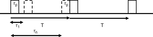
From Figure 4.17 the smallest time delay that can be distinguished between pulses is equal to τp, which for a monostatic radar gives a range resolution ![]() equal to:
equal to:
Any smaller delay than τp would result in the returned pulses overlapping.
The time delay resolution can also be related to the spectrum of the periodic train of pulses, which as can be seen from Figure 4.16 has discrete spectral lines occurring at multiples of ωo = 2π/T rad/s, and their amplitude is determined from the envelope of:
4.23 ![]()
where A is the amplitude of the pulse and n is an integer. The spectrum goes to zero at multiples of 1/τp Hz and the main lobe width is 2/τp. Taking the main lobe width B as the bandwidth of transmission, in a monostatic application Equation (4.22) gives a range resolution equal to:
4.24 ![]()
Thus the larger the bandwidth of the transmitted pulse train, the higher is the resolution between echoes. In the limit, the pulse train approaches a Dirac delta comb where all the spectral lines have equal amplitude given by 1/T. This is an advantage in sounder applications where the coherence between frequencies is evaluated as all the frequency components have the same amplitude, but in real systems only finite duration pulses can be generated and transmitted. Hence, it is usual to choose the pulse width such that the main lobe of the sin x/x function is within a certain percentage of its peak value over the frequency range of interest. For example, the required pulse width that corresponds to an amplitude drop to 0.99 ![]() requires a pulse width scaling factor of 1/1.315. Thus for a 1 µs pulse width, this corresponds to a bandwidth equal to 76.4 kHz instead of the 1 MHz bandwidth that corresponds to the zero crossings of the main lobe.
requires a pulse width scaling factor of 1/1.315. Thus for a 1 µs pulse width, this corresponds to a bandwidth equal to 76.4 kHz instead of the 1 MHz bandwidth that corresponds to the zero crossings of the main lobe.
4.7.1.2 Maximum Unambiguous Range
Due to the periodicity of the pulse, as can be seen from Figure 4.17, the largest time delay that can be measured without ambiguity is equal to the period of the waveform T. Thus the maximum unambiguous range Romax is given by:
4.7.1.3 Maximum Unambiguous Doppler Shift
In a pulse radar, the Doppler frequency or velocity of the target is measured either on a single pulse basis when ![]() or from the phase variations between consecutive pulses when
or from the phase variations between consecutive pulses when ![]() .
.
The derivation is similar to that presented in the CW section, except that in the periodic pulse case the received signal is limited in time to the duration of the pulse. Assuming monostatic radar and a single target the transmitted and received signals for a single pulse centred at t = 0 can be written as:
4.26 
where AT,R are the amplitude of the transmitted and received signals respectively and ![]() is the time-varying delay of the target, which includes the fixed range of the target and the change in range due to the velocity or movement of the target. Multiplying the received signal with a phase coherent replica of the transmitted carrier the output of the receiver can be expressed as:
is the time-varying delay of the target, which includes the fixed range of the target and the change in range due to the velocity or movement of the target. Multiplying the received signal with a phase coherent replica of the transmitted carrier the output of the receiver can be expressed as:
where p(t) is the pulse train and φo is the phase shift due to range.
Equation (4.27) indicates that the output of the receiver is an amplitude modulated sinusoid whose frequency corresponds to the Doppler frequency. If the Doppler frequency is high such that there are several cycles of it within ![]() then the Doppler frequency can be estimated from a single pulse. Otherwise several pulses would be needed to estimate the Doppler shift, as illustrated in Figure 4.18, which shows the difference between the two cases.
then the Doppler frequency can be estimated from a single pulse. Otherwise several pulses would be needed to estimate the Doppler shift, as illustrated in Figure 4.18, which shows the difference between the two cases.
Figure 4.18 Relationship between Doppler frequency and pulse period.
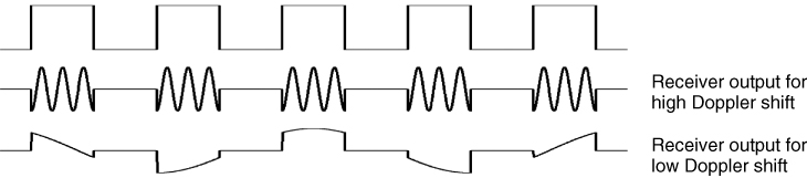
From Figure 4.18, the high Doppler shift produces several cycles within a single pulse, which for a single target can be analyzed using a simple zero crossing detector, but for multiple targets spectral analysis would be needed. For low Doppler shifts, the pulse train is seen to sample the Doppler frequency where the sampling theorem needs to be satisfied. Thus the maximum Doppler frequency ![]() that can be detected in this case is given by:
that can be detected in this case is given by:
where PRF is the pulse repetition frequency, which is equal to 1/T. For low Doppler shifts, the Fourier transform can be taken over a number of pulses.
Equation (4.28) could also be inferred from the spectrum of the pulse train shown in Figure 4.16, where the spectral lines are separated by 1/T Hz. To avoid ambiguity, this implies that the maximum allowable frequency shift is ±½T, which corresponds to half the frequency separation between two adjacent components.
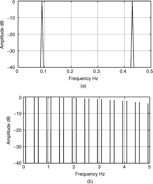
Equation (4.28) can also be related to Equation (4.27), which indicates that the spectrum of the demodulated signal consists of a sinusoid at the Doppler frequency convolved with the spectrum of the pulse train p(t) of the transmitted signal. Therefore in addition to the desired Doppler spectrum a number of unwanted components also appear as shown in Figure 4.19 for a PRF of 0.5 Hz and a Doppler shift of 0.08 Hz. The unfiltered signal is analyzed via the FFT and the spectral lines at the PRF are visible in addition to the wanted component, which can be eliminated by filtering up to 0.25 Hz for this example.
- Doppler resolution. The theoretical resolution of Doppler is related to the time window used in the spectral analysis, which is similar to the case of CW analysis. In the case of high Doppler shift, using a single pulse gives a very poor Doppler resolution as the pulse width is usually very small.
- Ambiguity function. Equations (4.28) and (4.25) are usually combined to give the limits of the ambiguity function defined in the following equation, which gives the time delay/range Doppler ambiguity of the waveform:

where u(t) is the complex lowpass representation of the bandpass transmitted signal.
Figure 4.19 Doppler spectrum estimated via the FFT: (a) frequency range up to PRF and (b) up to 10 PRF.
4.7.2 Factors Affecting the Resolution of Pulse Waveforms
Measurements of range and Doppler are affected by two factors:
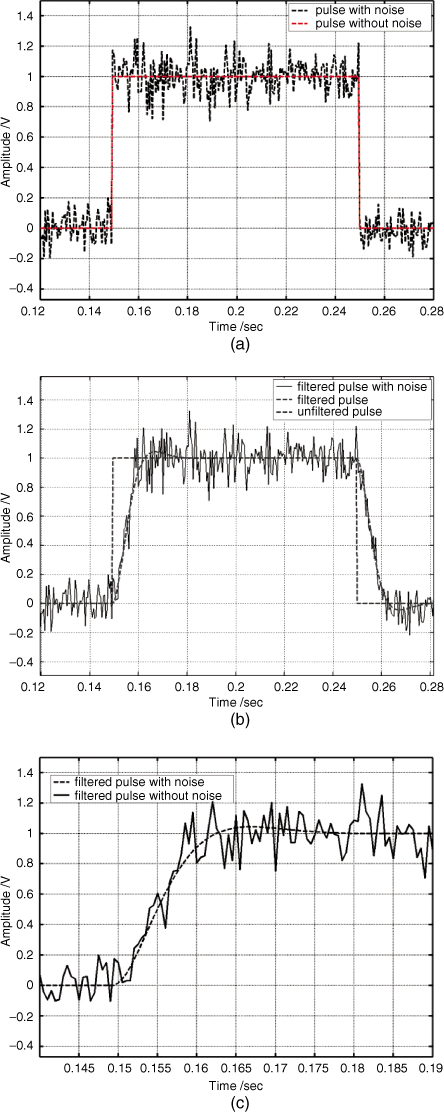
The bandwidth limitation can arise from two factors (i) the filters used to limit the transmitted spectrum to avoid interference to other users of the channel or (ii) the bandwidth of the channel in which the pulses have propagated, (see Section 3.3). Limited bandwidth affects the rise time of pulses whereas additive noise moves the edge of the pulse. A band-limited pulse corrupted by noise is displayed in Figure 4.20 with the ideal pulse shown for comparison. The figure shows that noise does not affect the rise time of an ideal pulse, as it does not have time to introduce perturbations to the sharp edge. Band limiting the pulse by means of filtering introduces a finite time duration known as transit time tr on the pulse to change between the low level and the high level. This in turn affects the accuracy of measuring the time at which the edge of the pulses crosses a certain threshold level. This impacts on the accuracy of measuring the range of the echo in the presence of additive noise.
Figure 4.20 Pulse corrupted with noise: (a) without band limiting, (b) with and without band limiting and (c) leading edge of band limited pulse with and without noise.
Doppler resolution can also be affected in the presence of phase noise where the spectral lines are broadened, which in turn affects Doppler resolution.
4.7.3 Typical Configuration of a Pulse Sounder
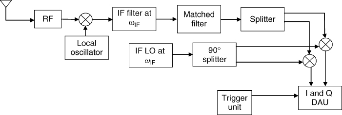
A typical block diagram for a pulse sounder is shown in Figure 4.21. To extract range and Doppler, the sounder extracts the quadrature components, which are lowpass filtered and logged for further processing.
Figure 4.21 Block diagram of a pulse sounder.
In a pulse sounder the data logger requirements are commensurate with the bandwidth of the transmitted pulse. For narrow bandwidth applications, this requirement can be satisfied with the off the shelf data acquisition boards. However, for ultra-wideband applications with bandwidths in excess of 500 MHz, which can extend up to several GHz, it is difficult to acquire the data at such high sampling rates. An alternative method would be to apply pulse stretching in the time domain to compress the bandwidth of the signal prior to digitization. This can be achieved by using a pulse generator with a different pulse repetition rate to mix with the incoming signal. For example, an ultra-wideband (UWB) pulse positioning system with 10 MHz PRF at the transmitter can use a PRF at the receiver that is offset by, say, 100 Hz. The impulse response is then obtained over 1,00,000 pulses (10 MHz/100), which corresponds to 10 ms. The requirement in such a system is that the response of the channel does not vary in this time interval or equivalently that the corresponding maximum Doppler shift that can be measured is limited to ±50 Hz. This technique has been widely used in mobile radio characterization with pseudo random binary sequences, as will be discussed in Section 4.8.
4.7.4 Practical Considerations for Pulse Sounding
A major consideration in pulse sounders is the high peak power required at the transmitter to increase the average transmitted power. In addition, due to the wide bandwidth of the transmitted signal, a pulse radar/sounder causes more interference to other channel users and its receiver is more susceptible to interference than a CW system.
Other considerations are the choice of the parameters of the pulse waveform that is the width of the pulse and the PRF. In radio channels such as the ionosphere, where the number of received echoes is a function of frequency and because the individual pulses suffer from elongation due to the variations of the group time delay, the transmitted pulse width and frequency have to satisfy certain conditions. The pulse width has to be chosen such that ionospheric phase distortion is minimized since the elongation of the pulse reduces its peak level and causes interference between the different received echoes. To satisfy these conditions it is usual in HF sounding of the ionosphere to choose pulse widths on the order of 10–50 µs. To cover the whole HF spectrum the frequency of the carrier is swept across the HF band 2–30 MHz.
Other issues that might affect the choice of the pulse waveform parameters is the maximum expected time delay of the farthest echo and the maximum expected Doppler shift. A high PRF covers a high Doppler shift but can lead to ambiguity in range as the far echoes fold on to the time delays of the near echo. On the other hand, a low PRF leads to folding of Doppler while providing range coverage. An example of such an application where the requirements of range and Doppler cannot be simultaneously met is HF radars, which are used for the detection of targets beyond the horizon and HF ionospheric propagation studies at high latitudes. HF radars are operated either in skywave mode to ranges of 100–4000 km or, over the sea, in surface wave mode to ranges from 10 km to 400 km. Applications of HF radars include ship and aircraft detection, iceberg detection, repeaters tracking and remote sensing of sea surface currents, winds and waves. In the application of sea state radar the Doppler shift from the sea return is very low and is on the order of a fraction of Hertz, and hence the radar PRF tends to be 2.5 Hz to cover the farthest sea echo return. However, a passing aircraft has a high Doppler shift, which smears the returns of the sea. Similarly, high latitude propagation suffers from high Doppler shift, which can be on the order of 100 Hz, while the sounder has to cover ranges that extend to hundreds of kilometres.
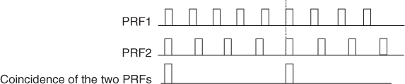
The PRF limitations can be overcome by switching the period from pulse to pulse or by using multiple PRFs where each PRF is transmitted over a certain period of time. This technique is known as staggered PRF or medium PRF [12, pp. 115–116]. For high latitude studies a pulse pattern with an interpulse period of 3 ms to cover the 100 Hz expected Doppler shift and extend the range over 48 ms to eliminate the range ambiguity has been proposed in [15, 16].
The multiple PRFs can be chosen either to provide unambiguous Doppler or unambiguous range. In Figure 4.22 an example of two pulse trains with high PRF where the ratio between the two PRFs is 5:6, that is the fifth pulse from one PRF, coincides with the sixth pulse from the second PRF. The high PRF provides adequate Doppler coverage where the range is then extracted from the spacing between the coincidence pulses, which is significantly longer than the interpulse duration of either PRF.
Figure 4.22 Staggered PRF structure for resolving the range Doppler ambiguity.
An alternative is to use multiple PRFs to extend the maximum detected velocity or Doppler shift. For multiple PRFs with a ratio as given by:
4.30 ![]()
where n1, n2, …, nN are integers, the maximum velocity vc that can be detected by the composite PRF is equal to:
4.31 ![]()
where vB is the ‘blind’ or ambiguous speed of the first PRF.
4.8 Pulse Compression Waveforms
To avoid the high peak power limitation of pulse systems, pulse compression techniques that transmit continuously can be used in radio channel measurements. The advantage of pulse compression waveforms can be seen from the radar equation [12]:
4.32 
for maximum range Rmax, where ![]() is the peak transmitted power,
is the peak transmitted power, ![]() are the gains of the receive and transmit antennas respectively,
are the gains of the receive and transmit antennas respectively, ![]() is the wavelength of the transmitted signal,
is the wavelength of the transmitted signal, ![]() is the cross section of the target,
is the cross section of the target, ![]() is the minimum signal to noise ratio, k is Boltzmann's constant, T is temperature in degrees and B is the bandwidth in Hz.
is the minimum signal to noise ratio, k is Boltzmann's constant, T is temperature in degrees and B is the bandwidth in Hz.
The radar equation implies that:
since for a pulse system ![]() , then:
, then:
![]()
Equation (4.33) shows that the maximum range can be increased either by increasing the peak transmitted power Ppk or by increasing τp. In a pulse system increasing τp reduces the time delay resolution unless the long pulse can be compressed to a narrow pulse to retain the resolution of the narrow pulse. If this can be achieved then the limitation of the required high peak power can be overcome, thus allowing the use of simple solid-state transmitters. These conditions can be met by pulse compression signals, which include phase coded sequences and frequency modulated continuous wave (FMCW) signals. These waveforms enable the estimation of the channel response or the detection of a target through their correlation properties.
Another advantage to using pulse compression waveforms is their interference rejection property. The receiver spreads narrowband interference while the wanted signal is compressed in time and is allowed to build up to its peak power, thereby giving a signal to interference advantage. This advantage led to the development of third generation mobile radio systems, which are based on code division multiple access, a technique that is based on pulse compression. Examples of interference effects on pulse compression waveforms are discussed in Section 4.19.7.
However, a major limitation of pulse compression systems is the required dynamic range since all the received echoes are added together and nearby echoes and clutter produce a higher received signal level than far away echoes due to the rn factor. This problem is referred to as the near-far problem in wireless communication systems.
4.8.1 Ideal Correlation Properties of Pulse Compression Sounding Waveforms
To identify the correlation properties of suitable pulse compression waveforms, a linear system's approach is considered herein as in Section 3.1. Ideally the sounding waveform is an impulse in time that has a flat spectrum over all frequencies. In real situations, the channel is limited in bandwidth and only a narrow pulse is required to cover the frequency range of interest. Instead of directly transmitting an impulse through the radio channel we measure the impulse response through the use of cross correlation between the transmitted signal and a replica at the receiver. This can be derived by considering the block diagram of Figure 4.23, where, for simplicity, the channel is considered as a linear time-invariant system with an impulse response equal to h(t). For an input z(t), the output y(t) is represented by the convolution integral as:
4.34 
To find the impulse response of the system, we define two correlation functions: the autocorrelation function of a signal x(t) and the cross correlation function of a signal x(t) with w(t):

where τ is the time delay between the signal x(t) and a delayed version of either x(t) or w(t) respectively. Generally correlation identifies the similarity between two signals as a function of displacement, which can be time delay as in Equations (4.35a) and (4.35b) or separation in distance or any other variable. For a time delay shift of zero, the autocorrelation function has its maximum value, which is equal to the energy E in the signal as given by:
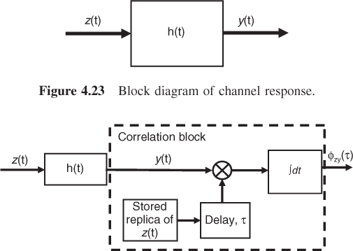
Referring to Figure 4.23, taking the cross correlation between the input z(t) and the output of the system y(t), as illustrated in Figure 4.24, and substituting for y(t) in terms of the convolution integral gives:
4.37 
Figure 4.23 Block diagram of channel response.
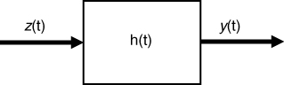
Figure 4.24 Block diagram of channel response followed by cross correlation (block within dashed line).
Exchanging the order of integration gives:

The inner integral in Equation (4.38) is the autocorrelation function φzz(τ − λ) of the signal z(t) as a function of the time delay or time shift variable τ − λ. Substituting the autocorrelation function in Equation (4.38) results in:
Equation (4.39) shows that if:
Equation (4.40) states that any waveform with an impulse autocorrelation function can be used to find the impulse response of the system by taking the cross correlation of the output of the system with a replica of the waveform at its input. Note that in Figure 4.24, the delay block forms the scanning parameter for the correlation function and thus it has to delay the stored replica by all values of τ to obtain the full correlation function. In a radar or sounder application, the aim is to measure the range of the target or the time delay of the multipath components. This is achieved by identifying the time delay τ that maximizes the expression in Equation (4.38) so that the received signal y(t) is coincident with the stored replica of the transmitted signal. This corresponds to the maximum at the zero time delay shift as given in Equation (4.36). By noting the delay value that maximizes the output the range of the target is identified.
The ideal correlation property in Equation (4.40) is generally difficult to realize. Considering the simple unity amplitude pulse waveform, its correlation is a triangular function with peak value equal to τp and width equal to 2τp. Thus any waveform that has correlation properties either close to the ideal impulse function or to the more practical triangular function can be used to estimate the channel response. While the ideal impulse function in Equation (4.40) can be realized by using a fully random generator with a white noise spectrum a practical implementation uses a binary pseudo noise sequence generator and other coded waveforms or alternatively uses FMCW signals, as will be discussed in Sections 4.9 and 4.10.
4.8.2 Pulse Compression Detectors
Two detectors can be used to implement the compression of coded or FMCW signals. One is based on the correlation detector in Figure 4.24 where the integrator can be implemented with a lowpass filter and the multiplier with a mixer, and the second method is based on matched filtering.
4.8.2.1 Correlation Detector
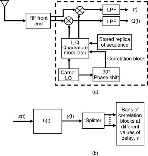
To estimate the magnitude and the phase for multiple echoes with different time delays the single correlation detector is usually implemented using a quadrature correlator as illustrated in Figure 4.25a and a bank of parallel correlation blocks (dashed blocks in Figure 4.25a) would need to be implemented for each expected multipath component as in Figure 4.25b. This architecture is not efficient in terms of hardware implementation. For example, to cover a 12 µs time delay window with a sample every 25 ns would require 480 correlation blocks. An alternative to employing a bank of correlation blocks for each time delay is to serially shift the time delay over a number of discrete time delay bins or to slide the time delay continuously as a function of time. The sliding correlator effectively performs ‘pulse stretching’ as the impulse response is obtained from a number of consecutive pulses. This in turn achieves bandwidth compression as will be discussed in Section 4.9 on coded pulse waveforms.
Figure 4.25 Block diagram of correlation detector for (a) single echo and (b) multiple echoes.
4.8.2.2 Convolution Detection with the Matched Filter
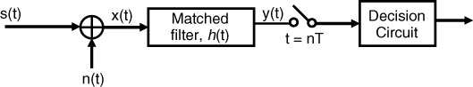
The correlation relationship in Equation (4.39) can be realized using the matched filter detector shown in Figure 4.26, which is normally used in digital transmission. Both the correlation receiver and the matched filter receiver aim to maximize the received signal energy at the instant of observation with respect to the average power of white Gaussian noise with zero mean and a double-sided power spectral density equal to No/2.
Figure 4.26 Optimum matched filter receiver for pulse compression waveforms.
To find the optimum impulse response for the matched filter h(t) consider the output of the filter due to the signal component:
4.41 
The noise output power is found by integrating the power spectral density of noise at the output of the filter, which is equal to the input power spectral density of noise No/2 multiplied by the magnitude squared of the filter response:
As in Figure 4.26 the optimum receiver only needs to maximize the peak of the output signal with respect to the average noise power at the instant of sampling, which occurs at multiples of T where T is the duration of the pulse waveform. This condition is expressed by:
To maximize Equation (4.43), use can be made of the Schwartz inequality for integrals of complex functions, which states that the area under the product of two complex functions is smaller than or equal to the area under the magnitude squared of each function. Assuming that ![]() is one function and
is one function and ![]() is the second function, then:
is the second function, then:
4.44 
where the equality holds when one function is the complex conjugate of the other, that is:
4.45 ![]()
Using Fourier transform properties this corresponds to a filter with an impulse response given by:
4.46 ![]()
Therefore, in the matched filter detector the received signal is passed through a filter specially designed to match the transmitted waveform s(t) by having an impulse response, which is the mirror image of the transmitted signal and delayed by T to ensure that the filter's response is causal.
By convolving the received signal with the transmitted signal, the output of the matched filter in the time domain due to the signal component is equal to:

where E is the energy of the signal.
Equation (4.47) also shows that the peak signal power to the mean noise ratio at the output of the matched filter at t = T is equal to:
4.48 ![]()
where from Equation (4.42) N = (E No)/2
Similarly, the correlation detector multiplies the incoming signal with a replica and integrates over the duration of the signal T to yield:
4.49 
In contrast to the correlation detector, which requires a bank of parallel detectors to obtain the impulse response of the channel for each time delay, the matched filter detector provides the impulse response of the channel in real time and thus only requires a single detector. For postprocessing and analysis, the output of the matched filter needs to be digitized using quadrature sampling to obtain the magnitude and phase of the channel response, as illustrated in Figure 4.27. Matched filtering can be accomplished using surface acoustic wave (SAW) devices. The SAW device has a limited time bandwidth product of the order of 10–300 and a bandwidth below 30 % of the IF of the device. The application of SAW devices for channel sounding has thus far been fairly limited to relatively small bandwidths on the order of 10 MHz and short duration pulses [17, 18].
Figure 4.27 Block diagram of matched receiver with quadrature sampling.
4.8.3 Comment on Pulse Compression Detectors
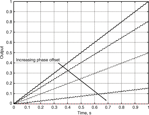
Although both the matched filter and the correlation detector outputs are identical at t = T, their instantaneous values are not equivalent for all time. Figure 4.28 shows an example of the matched filter and correlation detector waveforms where the output of the matched filter is seen to extend over twice the duration of the waveform. This is due to the convolution property where the duration of convolution of two waveforms of duration T1 and T2 is equal to T1 + T2. In contrast, at coincidence the correlation detector squares the signal and then integrates it to reach its maximum value at t = T. The output of both detectors varies with time and shows that lack of appropriate synchronization leads to deterioration in the performance of either detector. In addition, the correlation detector assumes that the locally generated signal is phase coherent with the incoming waveform. Figure 4.29 displays the deterioration in the output signal level of the detector due to a phase offset between the incoming carrier from the locally generated carrier by π/5, π/3, 0.45π and π/2. The signal is seen to go to zero when the two signals are in phase quadrature.
Figure 4.28 (a) CW pulse and its output from matched filter and (b) correlation detector.
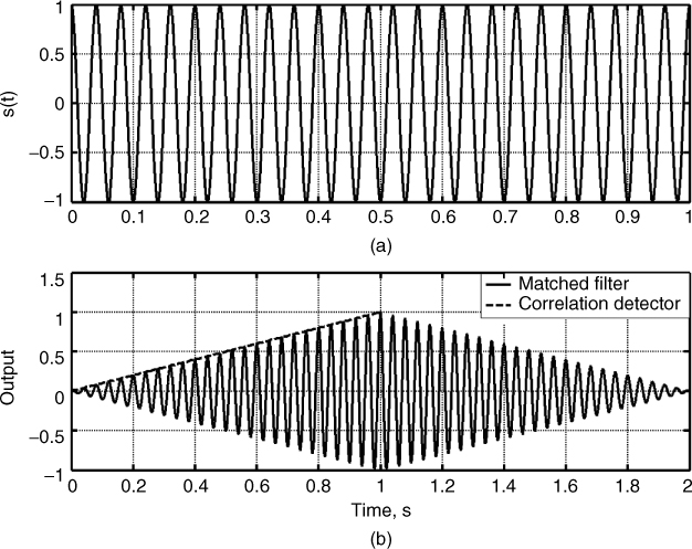
Figure 4.29 Correlation detector output with increasing phase offset between the incoming signal and the locally generated reference.
4.9 Coded Pulse Signals
Coded pulse compression signals use a binary sequence of length N bits each with duration equal to τp, which phase modulates a carrier. The most common is biphase modulation where each bit is coded with a phase difference of 180°. In this section, we study the correlation properties of the commonly used codes in radar and channel sounding, such as Barker codes, pseudo random binary sequences (PRBSs), Gold codes, Kasami sequences and loosely synchronous codes.
Considering the main parameters of interest in channel sounding or radar application, coded pulse transmissions have the following main properties:
Since in pulse compression the desired autocorrelation function of the waveform is an impulse function, deviations from the ideal give rise to limitations in the performance of the waveform when used for channel sounding or radar application. Such a limitation occurs if the autocorrelation function has a high sidelobe level with respect to the wanted main lobe. In the following discussion of the different codes, this property is studied in order to compare the performance of the different possible coded pulse transmissions. Another property that is of interest for simultaneous multiple antenna channel sounding is the cross correlation properties between various coded pulse sequences.
4.9.1 Barker Codes (1953)
To study the properties of the Barker codes, we will evaluate the autocorrelation function of the 13-bit Barker code as illustrated in Table 4.1. The code is biphase modulated and the autocorrelation function is obtained from the sequence defined by C = [1, 1, 1, 1, 1, −1, −1, 1, 1, −1, 1, −1, 1]. The values in the table are computed using the discrete correlation function given by:
Table 4.1 Correlation function for the 13-bit Barker code
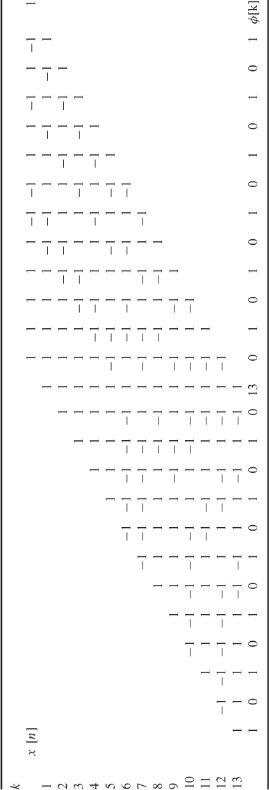
Equation (4.50) implies that for each value of k, the sequence x[n] is shifted by one location, multiplied by the corresponding value of the unshifted sequence, and added for all nonzero values. Table 4.1 shows the time shift of the sequence x[n] along the rows to generate x[r], which is multiplied by the value of the sequence for positive x[n] or the negative of the sequence when x[n] = −1. The result of the multiplication is added along the columns. Since the autocorrelation function exhibits even symmetry, the same result would have been obtained if the sequence was shifted to the right.
The table demonstrates the autocorrelation property of the Barker sequences where the ratio of the maximum of the correlation function to the sidelobe level is N. In general all the Barker codes have similar properties where the sidelobe level is down to 1/N where N is the length of the code, and since N = 13 is the longest Barker code that could be found with the same properties, the applications of the Barker code tend to be limited. Table 4.2 gives a list of all known Barker codes, their binary sequence and their sidelobe level in decibles. Figure 4.30 displays the correlation function for both the 13 bit code and the 7 bit code, which illustrate the correlation property of the code. The figure shows that the long sequence consisting of N bits has been compressed to give a peak with a base width equal to twice the bit duration with a peak level equal to N. An important property of such sequences is the ratio between the peak level and the level of sidelobes expressed in dB:
4.51a ![]()
![]()
4.51b ![]()
Table 4.2 All possible Barker codes
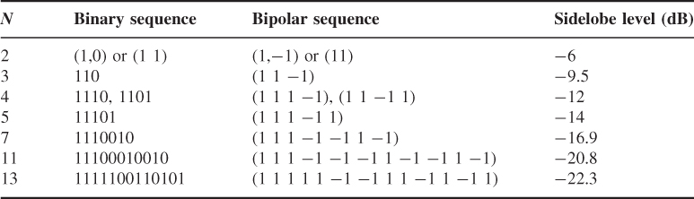
Figure 4.30 Autocorrelation function for (a) 13 bit Barker code and (b) 7 bit Barker code.
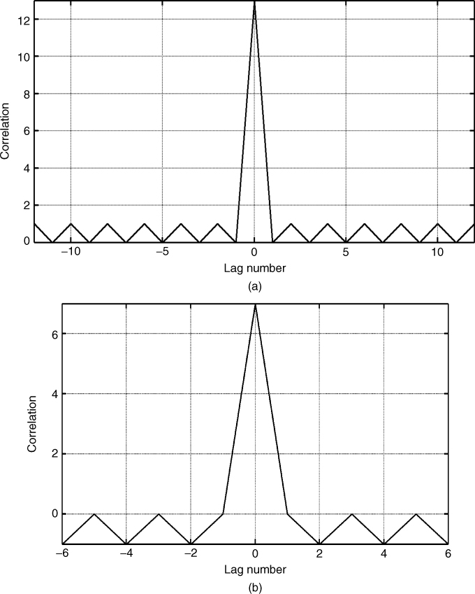
The normalized correlation function for the 13 bit code obtained by dividing the correlation function by φxx(0) is displayed in Figure 4.31a, where the sidelobe level is seen to be only 22.3 dB down from the main lobe. The presence of the sidelobes limits the dynamic range of echoes that can be observed without ambiguity since the sidelobes can obscure other echoes that might have time delays corresponding to the time lag of the sidelobe.
Figure 4.31 Properties of the 13 bit Barker code: (a) normalized correlation function of the code and (b) spectrum of the code.
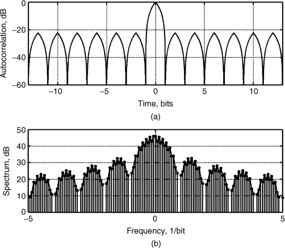
For radar/channel sounding the sequence is transmitted periodically, which results in a discrete spectrum with spectral lines occurring at multiples of the sequence length as shown in Figure 4.31b for the 13 bit code. Both the autocorrelation function and the spectrum in Figure 4.31 represent the 13 bit code interpolated by a factor of 100. The spectrum is also seen to have high sidelobes with the first sidelobe level at only about 14 dB down from the main lobe and the rate of decay of the sidelobes is only 6 dB/octave.
One limitation of the Barker codes is their short length, which limits the maximum time delay (range) of the echoes that can be detected unambiguously. Longer codes can be generated by nesting two shorter length Barker codes, using the Kronecker product ⊗ of the two codes. The resulting autocorrelation function depends on the order of computation of the Kroneckor product. Figure 4.32 displays the autocorrelation function on a linear scale for the bipolar nested 13 bit code with the 3 bit code for the two possible Kroneckor products, that is ![]() or
or ![]() where u, v represent the 13 bit code and the 3 bit code respectively. Note that the unipolar binary correlation function would have resulted in a reduced correlation coefficient that depends on the number of 1's in the sequence.
where u, v represent the 13 bit code and the 3 bit code respectively. Note that the unipolar binary correlation function would have resulted in a reduced correlation coefficient that depends on the number of 1's in the sequence.
Figure 4.32 Nested Barker codes: 13 bit code (long) with 3 bit code (short), ---code = [short;short;short;short;short;-short;-short;short;short;-short;short;-short;short]; and __code = [long; long; -long].
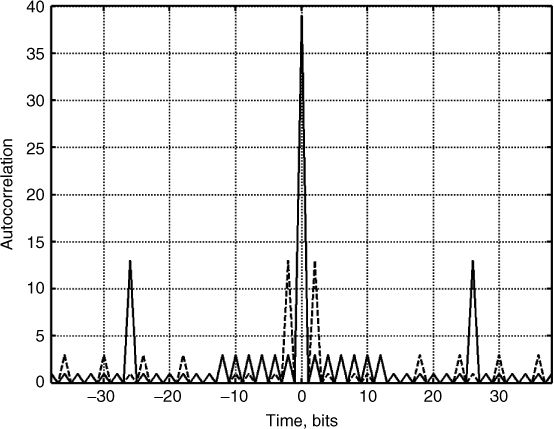
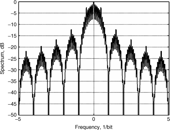
Figure 4.32 shows that the resultant code has an autocorrelation function with a peak value equal to the length of the code, N = 39, which is 9.5 dB higher than the 13 bit code and with sidelobe levels either equal to 3 (−22.3 dB) or 13 (−9.5 dB), which are commensurate with the lengths of the constituent codes. Using the long code with the first sidelobe level at bit 26, the maximum detected range is extended to twice the value of the original 13 bit code with similar sidelobe suppression. The corresponding nested code spectrum shows similar sidelobe levels as the original 13 bit code with 2 dB deterioration and more irregular peaks, as shown in Figure 4.33.
Figure 4.33 Spectrum of nested Barker code.
4.9.2 PRBS Codes
To obtain higher processing gain maximal length codes, referred to as m-sequences or pseudo random binary sequences (PRBSs), also known as linear recursive sequences (LRSs), can be generated using a shift register with appropriate feedback. Mathematically they are derived on the basis of irreducible polynomials over the Galois field, GF(2k), where k is the length of the shift register. The generalized architecture for the polynomial is based on modulo 2 addition, delay elements and feedback, as shown in Figure 4.34.
Figure 4.34 Block diagram of the generator polynomial of m-sequences.
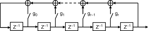
In the figure, z−1 is a unit of time delay and the addition is modulo 2. That is the output is equal to 1 if the inputs are 1, 0 or 0, 1 and 0 if the inputs are 0, 0 and 1, 1, where the latter gives a 0 with a carry output of 1, which is not carried forward. The generalized polynomial, g(z) is written as:
4.52 ![]()
where the coefficient gr is always equal to 1 and the remaining coefficients gi are 1 or 0. The output can be either delayed by a number of taps or it can be taken directly from the last register. For example, if the coefficients are [1 0 0 0 0 1 1] this represents a polynomial of order r = 6. This is equivalent to a polynomial with coefficients [0 5 6] as in:
4.53 ![]()
The length of the shift register k determines the length of the code N, which is given by:
4.54 ![]()
Two conditions must be met to ensure proper generation of the sequence:
Figure 4.35a gives the theoretical feedback connections for k = 9 or equivalently for the 511 bit code. The modulo-2 addition can be implemented with an exclusive OR (XOR) gate. A practical implementation using off the shelf transistor–transistor logic (TTL) devices is given in Figure 4.35b, where the outputs of all the 9 bit registers are fed into two 5 input NOR gates in the 74260 IC and these are then fed into an AND gate to detect the all-zero state. This is then fed to an OR gate with the feedback from the XOR gate, which gives a 1 when either bit 9 or bit 5 is equal to 1. In this configuration the register starts from the zero state using the clear signal, as shown in Figure 4.35c, which shows the simulation timing waveforms of the circuit. The all-zero state is detected by the feedback loop and an initial seed of 1 is fed to the input of the shift register. The circuit can also be easily implemented on gate arrays using VHDL code.
Figure 4.35 (a) Theoretical m-sequence generator, (b) schematic of implementation and (c) timing waveform for implementation in (b).
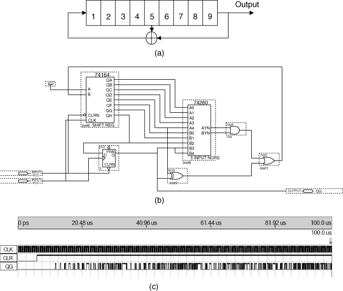
Table 4.3 gives a list of some of the possible m-codes and the feedback connections while Table 4.4 gives the length of the sequence for a number of shift registers and the number of possible sequences. The total number M of maximum length sequences that might be obtained from a k-stage generator is:
4.55 ![]()
Table 4.3 Order of polynomial and generating polynomial for m-sequences

Table 4.4 Length of sequence and number of possible m-codes versus number of stages
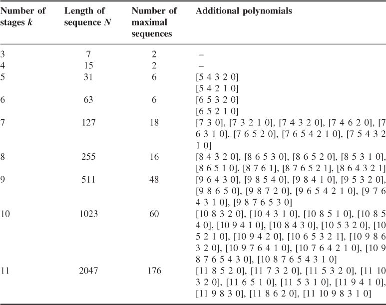
where pi are the prime factors of N. This is useful for applications where the same length sequence is required. Some of the additional polynomials that can be used are listed in Table 4.4. In general each sequence has a reverse sequence that can be generated from the same polynomial. For example, for the polynomial [10 8 3 2 0], the reverse polynomial is [10 2 7 8 0] where each coefficient is subtracted from r except for the end terms.
Figure 4.36 displays the spectrum of a PRBS sequence that is seen to have the envelope of a (sinx)/x function with spectral lines separated by WRF = 1/(![]() ) Hz.
) Hz.
Figure 4.36 Spectrum of m-sequence showing (a) the sinx/x envelope and (b) illustration of the spectral lines separation.
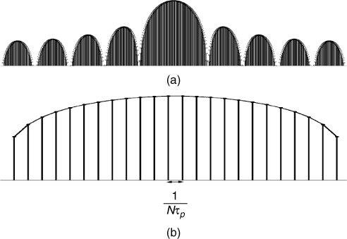
M-sequences are called pseudo random sequences because they fit many of the tests of randomness, which are:
Taking the example for r = 3, the generated sequence is [1 0 0 0 1 1 1 1 0 1 0 1 1 0 0], which has seven zeros and eight ones (property one). The runs of zeros and ones are [0 0 0] [0 0] and 2 [0], and 2 of [1] [1 1 1 1] [1 1] respectively, which gives a total number of runs equal to 8. Runs of length 1 are 4, which correspond to half the number of runs. Runs of length 2 are 2, which is one-fourth the number of runs, and the number of runs with 3 and 4 is one each. The correlation property can be seen from Table 4.5 where the original sequence in the first row is compared with the cyclic version of itself. The number of agreements minus the number of disagreements for each row when compared with the first row is always equal to −1 or −1/15. After 15 shifts the shifted sequence is coincident with the original sequence and gives a maximum of 15/15, which is equal to 1.
Table 4.5 PRBS code and cyclic shifted version illustrating the correlation property of the code
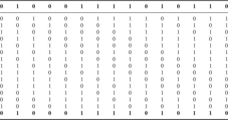
For biphase modulation the 1's are represented by +1 and the 0's are represented by −1. The resulting autocorrelation function is given by [19]:
4.56 
For long sequences, the theoretical peak sidelobe level is about 1/N with respect to the main lobe. An example of the aperiodic autocorrelation function is shown in Figure 4.37 for a 63 bit long sequence where the level of the highest sidelobe is about −17.99 dB down from the main lobe. The periodic autocorrelation function for the same sequence (obtained over 36 periods) is displayed in Figure 4.37b where the level of the sidelobes is considerably reduced and approaches the theoretical −20log10N value, which is −35.98 dB for the given 63 bit sequence. The ideal periodic autocorrelation function can be, however, obtained by using the FFT due to the periodic nature of the FFT. This is achieved by taking the inverse FFT of the sequence, followed by taking the FFT of its magnitude. The ideal autocorrelation function is then obtained by taking the magnitude of the resultant. For multiple antenna applications, orthogonal multiple codes are needed for simultaneous transmission. In this case the cross correlation property of the sequences needs to be evaluated. Figure 4.37c displays the cross correlation between two PRBS sequences generated by taking the reverse sequence and a different polynomial of the same length. It can be seen that the level of the unwanted component level can be as high as −12 dB, which limits the dynamic range of the detected multipath components in a channel sounding application.
Figure 4.37 Autocorrelation function for a 63-bit sequence in dB: (a) aperiodic, (b) periodic and (c) auto-correlation and cross-correlation of a 255 bit sequence with its reverse sequence and a different polynomial.
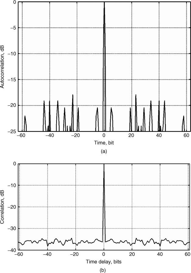
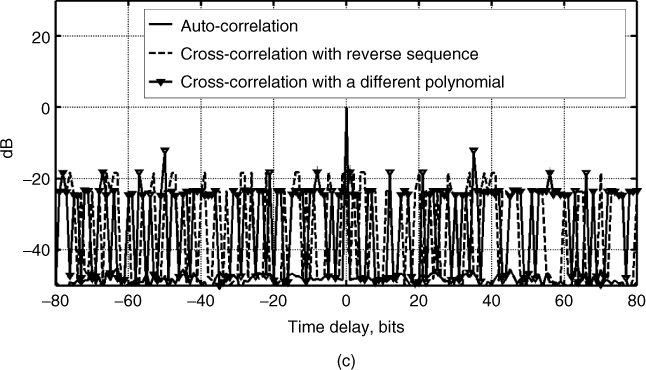
4.9.3 PRBS Related Codes: Gold Codes
A family of sequences, which can be derived from m-sequences is the Gold sequences proposed by Gold in 1967 and 1968. Gold sequences are used for their cross correlation property where each sequence is orthogonal to every other sequence in the set. Gold sequences have the property that the cross correlation between any two, or between shifted versions of the codes, takes on one of three values: −t(k), −1 or t(k) − 2, where k is the length of the register:
4.57 ![]()
They are derived by modulo-2 addition using an XOR gate of two m-sequences, as shown in Figure 4.38. The two PN sequences u and ν are called a preferred pair of sequences and the resulting sequence has the same period as the original sequences. The requirements for a pair of sequences u, ν of period N = 2k − 1 to be the preferred pair are as follows:
- k is not divisible by 4,
- ν = u[q], where q is odd, q = 2k + 1 or q = 22k − 2k + 1,
- ν is obtained by sampling every qth symbol of u,
Figure 4.38 Block diagram representation of a Gold sequence generator.

For the sequences u and ν, a set G(u, ν) of Gold sequences is defined by:
4.58 ![]()
where T represents the operator that shifts vectors cyclically to the left by one place and ![]() represents addition modulo-2. The set G (u, v) contains N + 2 sequences of period N. Table 4.6 gives a list of some of the preferred polynomial generators for a few Gold sequences.
represents addition modulo-2. The set G (u, v) contains N + 2 sequences of period N. Table 4.6 gives a list of some of the preferred polynomial generators for a few Gold sequences.
Table 4.6 List of some of the preferred polynomials for Gold codes
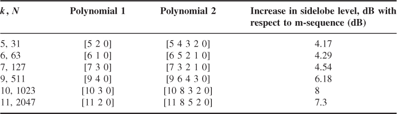
Figure 4.39 displays the autocorrelation of a 63 bit Gold sequence generated from the polynomials listed in Table 4.6. Compared with Figure 4.37, the sidelobe level is seen to be higher by about 4.17 dB, which is undesirable for the detection of multipath as it reduces the dynamic range of detected echoes. The increase in the sidelobe level with respect to the original preferred polynomials is tabulated in the last column of Table 4.6.
Figure 4.39 Autocorrelation of a 63-bit Gold code.
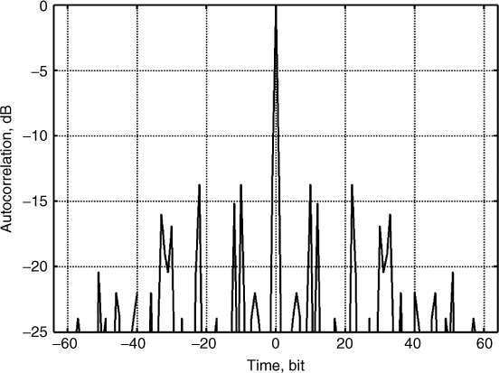
4.9.4 Kasami Code
Kasami sequences are a set of sequences that have good cross correlation properties. There are two classes of Kasami sequences: the large set and the small set, which is a subset of the large set. Only the small set matches Welch's lower bound for correlation functions that establishes how small the cross correlation and autocorrelation can be for a set of sequences [20, 21]. Similar to the m-sequence, Kasami sequences have period N = 2k − 1, where k is a nonnegative even integer. The small set of Kasami sequences is obtained from modulo-2 addition of m-sequence u of length N, and a time shifted version of a sequence w obtained by decimating u by 2k/2 +1 using Equation (4.59), in which T denotes the left shift operator, m is the shift parameter for w and ![]() denotes addition modulo-2:
denotes addition modulo-2:
The small set contains a total of 2k/2 sequences for k even values only. The correlation between different Kasami sequences or its delayed sequences have only three values, {−1, –s(k), s(k) − 2} which are relatively low values for a code length of 2k − 1, where s(k) = 2k/2 + 1. Table 4.7 gives some of the polynomials that can be used to generate the small set of Kasami codes and the corresponding sidelobe level estimated from simulation as shown in Figure 4.40 for the code with k = 12. Long Kasami codes can be used for channel sounding depending on the required dynamic range needed for the measurements.
Table 4.7 Kasami code generator polynomial and corresponding sidelobe level
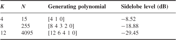
Figure 4.40 Autocorrelation function of a 4095 bit Kasami code.
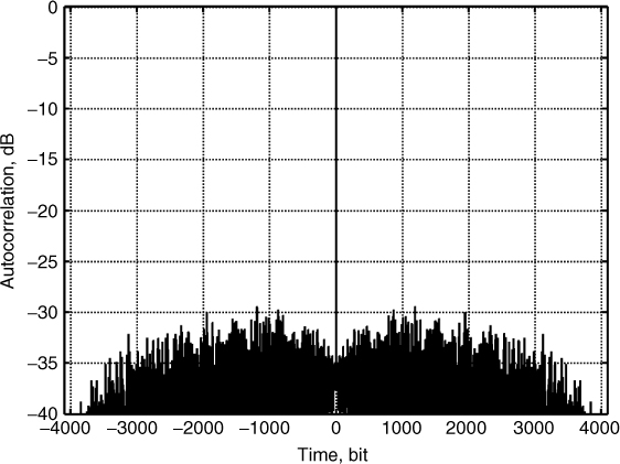
4.9.5 Loosely Synchronous Codes
Loosely synchronous codes are codes generated by inserting zeros in between Golay complementary codes C and S, as shown in Figure 4.41. The generated codes have the following correlation properties:
4.60 
Figure 4.41 Composition of loosely synchronous codes.
where Cn,m is the mth symbol in the nth loosely synchronous sequence set, τ is the time delay and IFW is the interference free window, which is equal to 2τIFW. The IFW is a function of the number of sequences transmitted in parallel, and this in turn limits the maximum time delay window that can be measured. For example, for a pair mate with length 2L and L − 1 zeros, the total length of the sequence is 4L − 2, and the τIFW = L − 1 [22]. Loosely synchronous codes can thus be used for a limited number of multiple antenna channel sounding applications [23].
4.10 Serial Correlation Detection of Coded Transmission
In Section 4.8 it was shown that the long code is compressed in time to a narrower pulse by using correlation detection. In radio channel sounding a correlator would be required for each time delayed echo. This gives a large overall number of correlators to cover the time delay window. This approach originally implemented by Price and Green [24] in the RAKE receiver architecture, is inappropriate to realize due to the high level of complexity. The correlation detector compresses the signal in time but not in bandwidth. If the bandwidth of the transmitted sequence is moderate it is possible to digitize the received signal prior to correlation and to perform the correlation using digital processing techniques either in hardware such as in gate arrays and dedicated digital signal processing chips or in software using various programming languages [25]. The use of either technique depends on whether real time monitoring of the channel is required or offline processing is sufficient.
Another approach to avoid the implementation of parallel correlators is to use a serial correlator to obtain the impulse response sequentially using either a continuous time sliding correlator or a discrete stepped cross correlator to cover the required time delay window. Inherent in the serial cross correlator is time scaling, which results in bandwidth reduction. Both techniques are outlined below.
4.10.1 Sliding Correlator
Since its introduction by Cox in 1972, the sliding correlator shown in Figure 4.42 has become the most used method of bandwidth compression of phase coded transmission [26]. It accomplishes this by using a different clock rate of the shift register in the sequence generator at the receiver, equal to fck(1 −1/K) or fck − Δf, where K is chosen appropriately to ensure sufficient bandwidth compression with minimum distortion to the compressed pulse. The impulse response of the channel emerges at the output of the receiver over K snapshots. By elongating the time required to obtain the impulse response by a factor equal to K, the bandwidth of the received signal is reduced by K. The reduction in the required speed of the ADCs is accompanied by a loss in the sampling rate of Doppler. For example, a channel sounder with a 10 MHz clock rate and a requirement to cover a 12 µs time delay window with a sample every λ/3 (5 cm at 2 GHz carrier), with a 5000 compression ratio (that is 2 kHz frequency offset), would take 60 ms to generate each impulse response. This corresponds to a maximum vehicle speed of 3 km/h, which would be difficult to maintain in traffic conditions.
Figure 4.42 Block diagram of a sliding correlator.
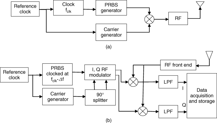
With the advent of fast ADC, the sliding correlator became less popular as high bandwidths can be digitized with off the shelf data acquisition cards. However, with the new applications of ultra-wideband signals, the sliding correlator is being revisited as a valuable bandwidth compression technique.
The output of the sliding correlator consists of the wanted compressed signal plus an in-band unwanted component that cannot be removed by filtering. This effect is expressed by:
4.61 ![]()
where ![]() represents the filter frequency response,
represents the filter frequency response, ![]() the wanted compressed component and
the wanted compressed component and ![]() represents the unwanted component [27].
represents the unwanted component [27].
To remove the unwanted term, it is recommended that the spectrum of the sequence be filtered prior to transmission as well as the reference sequence prior to correlation. The filters cut-off frequencies are chosen to be related to the clock frequencies of the sequence generators at both the transmitter and receiver and the cut-off frequency of the LPF at the output of the receiver is chosen appropriately to exclude the unwanted component. This retains the theoretical dynamic range of the sequence as determined by the ratio of the peak to sidelobe level. In channel sounding, it is usual to filter the sequence prior to transmission to reduce the effect of interference to other users of the channel. The filter's bandwidth is chosen to enclose the first nulls of the spectrum, which for a PRBS sequence is equal to twice the clock rate, 2fclk. So for a 10 MHz clock rate the PRBS spectrum is filtered with a 20 MHz filter, centred at the carrier frequency. By filtering the PRBS sequence at the receiver, for example using a filter with a bandwidth equal to 2(fclk + Δf) and choosing the cut-off frequency of the LPF filter that excludes the unwanted component, the reduction in the dynamic range can be avoided. This condition is met when the cut-off frequency of the filter is chosen to exclude the minimum frequency of the unwanted component, which is given by [27]:
4.62 ![]()
where β and β′ are the factors for the filters used for filtering the PRBS sequences at the transmitter and receiver respectively and:
4.63 ![]()
Choosing the same filtering factors gives the design equation:
4.64 ![]()
which for the usual factor of 2 gives:
4.65 ![]()
The corresponding LPF cut-off frequency is then approximately equal to ![]() .
.
The filtering of the PRBS sequence reduces the time delay resolution of the sounder, but this is generally inevitable because for interference reduction the spectrum of the transmitted signal has to be limited.
4.10.2 Stepped Cross Correlator
The sliding cross correlator requires the generation of two different clocks that differ slightly in frequency and have to be stable with time. This can be avoided by clocking both sequences at the transmitter and at the receiver at the same rate with the receiver's sequence delayed by a variable digital delay to cover the whole time delay window [28]. To permit adequate sampling of the power delay profile, a sample every 25 ns gives four samples per bit for a 10 MHz clock rate. To cover 12 µs, 480 steps or 5.76 ms are required to complete one power delay profile when a single correlator is used. Therefore, vehicle speeds up to 31.25 km/h permit the measurement of a power delay profile every 5 cm. Faster vehicle speeds can be achieved by increasing the number of correlators and performing parallel processing on the four samples per bit. This, however, is achieved at the expense of added complexity.
4.11 Comment Regarding Coded Transmission
In coded transmission as in the single pulse sounding, the bit duration and the period of the code need to be chosen appropriately depending on the channel to be measured. For mobile radio applications, pulse dispersion is not an issue as in ionospheric sounding, where the code length is limited by the instability of the propagation conditions and the bit length is determined by frequency dispersion [29, 30]. In their ionospheric sounding measurements using coded pulse transmission, Coll and Storey [31] concluded that coded pulse compression worked efficiently under stable conditions and at frequencies removed from the critical frequencies. Due to the frequency dispersion effects, sequences with different bit rates can be transmitted to obtain the optimum bandwidth for compression [29]. To obtain ionograms the carrier frequency of the code has to be swept across the HF spectrum.
4.12 Frequency Modulated Continuous Wave (FMCW) Signal
Another waveform that is suitable for pulse compression is the FMCW signal, also known as chirp. A chirp sounder or radar transmits a frequency modulated signal that is characterized by a linear frequency increase or decrease over a frequency range of B Hz in T seconds, where B/T Hz/s is known as the sweep rate and the time bandwidth product BT is the dispersion factor. Mathematically a chirp signal is expressed as:
where ωc is the carrier frequency in radians/s and χ = π(B/T). Its corresponding spectrum is given as:
4.66b 
where C and S are the Fresnel integral [32]. At the centre frequency of the sweep the magnitude of the spectrum is equal to ![]() . For large time bandwidth products the phase due to the Fresnel integral terms in Equation 4.66a is equal to –π/4 and the magnitude of the spectrum, which can be considered to be a constant, is represented by:
. For large time bandwidth products the phase due to the Fresnel integral terms in Equation 4.66a is equal to –π/4 and the magnitude of the spectrum, which can be considered to be a constant, is represented by:
4.67 ![]()
where ωc is assumed to be zero for mathematical convenience.
The amount of energy outside B is a function of the dispersion factor, where for BT = 10 and 100, 95 and 98–99 % of the signal energy is contained within B respectively [32]. For practical applications of radars and sounders, BT values are much higher than this and thus the spectrum can be considered to be contained within B.
Figures 4.43 and 4.44 display the time domain representation of a chirp signal with a 50 Hz bandwidth and 2 second duration with its corresponding spectrum shown in Figure 4.45.
Figure 4.43 Frequency time relationship of a linear frequency modulated, chirp signal.
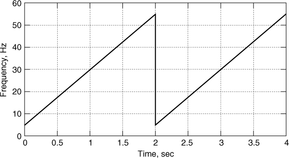
Figure 4.44 Time domain waveform versus time of a linear frequency modulated, chirp signal.
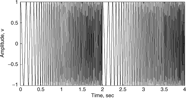
Figure 4.45 Spectrum of the chirp signal with 50 Hz bandwidth and 2 second duration.
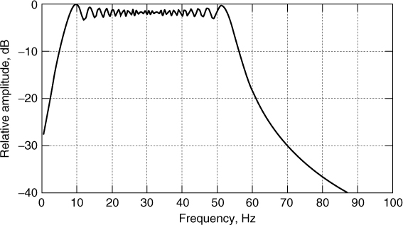
Unlike the PRBS code the spectrum of the chirp signal is contained within the frequency range of the swept bandwidth and therefore does not require filtering prior to transmission. However, similar to the PRBS code the chirp signal can be compressed either via a matched filter or a correlation detector.
4.12.1 Matched Filter Detector
The matched filter equation for a chirp signal is given by:
which represents a chirp signal with an opposite slope to the transmitted signal. Figure 4.46a and b displays the matched filter impulse response for a chirp signal with positive slope. Effectively the matched filter accomplishes time compression by delaying the frequencies in the reverse order to its input, thereby bringing all the frequencies back in phase.
Figure 4.46 Matched filter response: (a) impulse response and (b) response to a matched chirp signal.
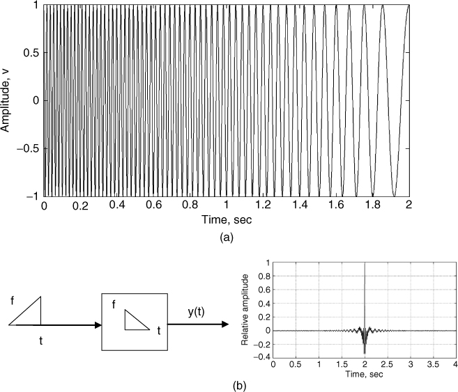
The output of the matched filter y(t) is found by convolving the chirp signal with the matched filter response, which gives the compressed pulse:
4.69 ![]()
Detailed analysis of the matched filter detector can be found in [32]. Equation (4.68) shows that the compressed pulse has a peak signal level equal to 10 log(BT) and that the envelope of the compressed signal is of the form of a sin x/x function, as shown in Figure 4.46b rather than the ideal impulse function required for channel sounding. It also differs from the triangular waveform, which corresponds to the compressed PRBS signal. Figure 4.47 shows that for a chirp signal with a 50 Hz bandwidth and 2 second duration, the rate of decay of the sidelobe level is 6 dB per octave and the 4 dB width of the main lobe is equal to 0.02 seconds, which corresponds to ∼1/B Hz. For large time bandwidth products the sin x/x envelope can be considered as the Fourier transform of a rectangular pulse over the bandwidth of the chirp signal. The sin x/x shape of the compressed chirp signal in time is similar to the envelope of the spectrum of the PRBS sequence. While the spectrum of the PRBS signal is filtered to limit its bandwidth, the envelope of the chirp signal can be shaped to reduce the level of the time domain sidelobes of the compressed signal. This is important in channel sounding or radar applications as the sidelobes amount to leakage from one echo to the other echoes, which are delayed from it in time and obscure the resolution of multipath.
Figure 4.47 Compressed sinx/x envelope of a chirp signal in time, illustrating (a) rate of decay of sidelobes and (b) width of the main lobe.
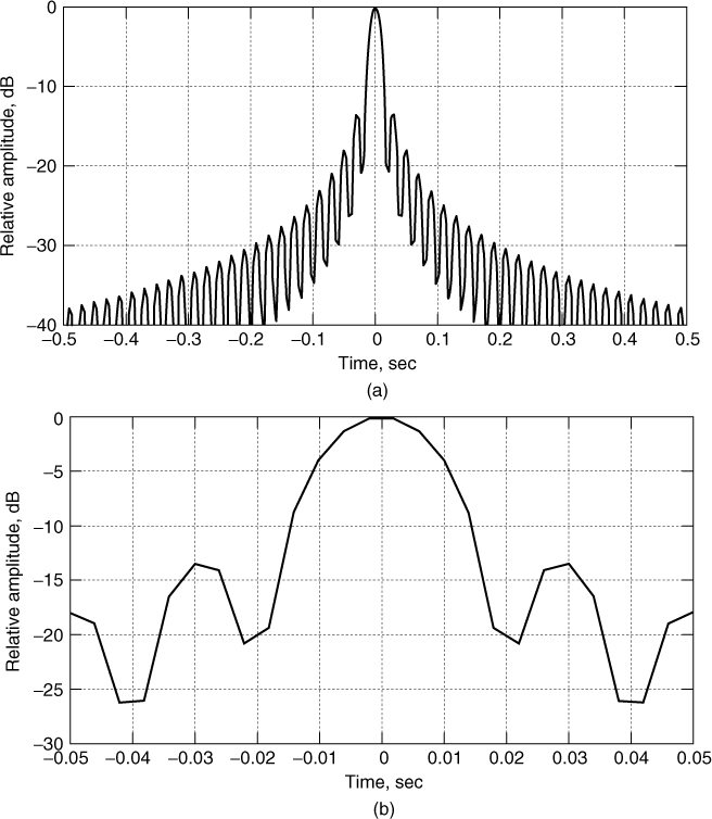
The high sidelobe levels can be reduced by: (i) weighting the transmitted or received signal either in the time domain or in the frequency domain by using various weighting functions such as the Hamming window, Taylor window or Gaussian window [33] or by (ii) transmitting a nonlinear FMCW signal [34, p. 106] . Thus, although theoretically the time delay resolution of a chirp signal is 1/B second practically it depends on the window function used to reduce the sidelobes of the compressed signal, as will be discussed in Section 5.2. For frequency dispersive channels such as the ionosphere the compression is also a function of the slope of the group time delay as a function of frequency [33, 35, 36]. Since the chirp signal repeats every T seconds its maximum time delay coverage is equal to T and its maximum unambiguous Doppler coverage is equal to ± 1/(2T) Hz.
4.12.2 Heterodyne Detector of FMCW Signals
An alternative to the matched filter detector is the detector illustrated in Figure 4.48 where the received signal ![]() is multiplied by a delayed replica of the transmitted signal
is multiplied by a delayed replica of the transmitted signal ![]() lowpass filtered and the output of the receiver
lowpass filtered and the output of the receiver ![]() is then spectrum analyzed to achieve the sin x/x compression [37].
is then spectrum analyzed to achieve the sin x/x compression [37].
Figure 4.48 Block diagram of heterodyne/homodyne detector.
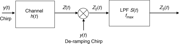
Assuming that the channel has an ideal impulse response that essentially delays the signal and multiplies it by a constant, the mixer's output Z2(t) prior to filtering consists of two beat notes, as shown Figure 4.49, where the low frequency component is proportional to the time delay between the received chirp signal and the locally generated signal, and lasts for T − τo, and a high frequency HF component produced for τo. By removing the HF component with the lowpass filter the low frequency component can be related to the time difference between the two signals by (B/T)τo. Thus the filter cut-off frequency fmax is chosen to accommodate the time delay τmax of the farthest echo with frequency fmax = (B/T)τmax.
Figure 4.49 Graphical representation of the output of the mixer in Figure 4.48.
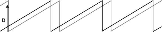
For a multipath radio channel or for a radar application with multiple targets, the received signal can be represented by the sum of delayed and attenuated replicas of the chirp signal. Thus analytically the output of the detector can be represented by:
4.70 ![]()
where
![]()
and Ai and τi are the amplitude and time delay of the ith component.
For each multipath component, the output of the mixer can be represented by:
4.71 
The first term is at twice the carrier frequency and is filtered out by the LPF, leaving the second term, whose frequency is given by:
4.72 ![]()
If the receiver is moving at a constant speed ν, then the time delay of the received echo is varying with time and the output frequency of the detector can be represented by [37]:
4.73 ![]()
where
![]()
and ![]() is the time delay due to the range of the target.
is the time delay due to the range of the target.
For relatively small vehicle speeds with respect to the speed of light, the instantaneous frequency ![]() within a pulse reduces to:
within a pulse reduces to:
where the first term is a frequency component due to the Doppler shift and the second component is the frequency offset due to the time delay of the echo.
In channel sounding and radar applications it is assumed that the Doppler shift within the duration of a single sweep is much smaller than the time delay component and that the measured frequency on a sweep basis is predominantly proportional to the time delay or range. Measuring the frequency on a sweep basis gives a sin x/x envelope with a bin width equal to 1/T Hz in frequency or 1/B seconds in time delay. For a Doppler component that is smaller than ± 1/(2T) Hz, the measured frequency remains within the same frequency bin (also referred to as the range bin or time delay bin) and hence provides a direct measurement of the time delay. For higher Doppler shifts, the measured frequency moves to a different range bin, which results in ambiguous estimation of the range of the echo. This effect is known as the range/Doppler ambiguity of FMCW radar and requires advanced waveform design (see Section 4.13).
Analyzing a number of consecutive sweeps, the propagation time delay in the nth sweep would have increased by nT, as expressed by:
4.75 ![]()
This results in a measured frequency equal to:
By comparing Equations (4.76) and (4.74), the frequency in the nth sweep, fin, is seen to have the additional term B(ν/c)n, due to the movement of the target over the duration of the n sweeps. Since the ratio of the velocity of a mobile or a target in a radar application is much smaller than the speed of light, it can be assumed that generally the measured frequency on a pulse basis is due mainly to the range or the time delay. For large values of n and high bandwidths, this additional term would need to be considered.
In both radar and channel sounding applications, the aim is to measure the range or time delay, Doppler shift and relative amplitude of the echoes. The analysis so far shows that spectral analysis on a sweep basis enables the estimation of the range or time delay of the multipath components and their relative amplitude. Assuming that the Doppler shift is restricted to ± 1/(2T) Hz, the Fourier transform on a single sweep is given by [37]:

4.77b 
where
That is the Fourier transform over a single sweep gives a sin x/x function centred at the frequency, which corresponds to the time delay between the transmitter and the receiver chirp signals. While the output of the detector can be observed on a spectrum analyzer for online processing it is commonly digitized at a sampling frequency fs chosen to be greater than 2fmax and spectral analysis is performed using the FFT algorithm. The result of the first FFT is a number of range bins extending in frequency from zero to half fs. Thus for M time samples per sweep a total of M/2 samples are retained. These can be scaled to the time delay using the sweep rate B/T according to τi = (T/B)fi.
To measure the Doppler shift and time variability of the channel, analysis over a number of sweeps would be necessary. Equations (4.77a)-(4.77c) show that the phase shift term is a function of the Doppler shift. By taking the Fourier transform over N sweeps at the mth range bin, the spectrum is also of the form of a sinx/x function with frequency centred at the Doppler shift frequency as given by [37]:
4.78a ![]()
where
The matrix in the following equation illustrates the two-dimensional array that results from the FFT processing:
4.79 
where first each sweep is processed to give amplitude versus range and then processing over a number of sweeps gives the amplitude versus Doppler and range [37].
An example of a double FFT processing on FMCW data obtained in an indoor sounding experiment is displayed in Figures 4.50 and 4.51. In Figure 4.50, following the first FFT, the multipath components are resolved in a time delay over a number of sweeps. The second FFT is then performed on each time delay over the one second interval to obtain the time delay Doppler function displayed in Figure 4.51. In addition to estimating the Doppler shift, the second FFT is seen to enable the further resolution of multipath components that have the same time delay but arrive from different angles.
Figure 4.50 Time variant multipath structure after the first FFT.
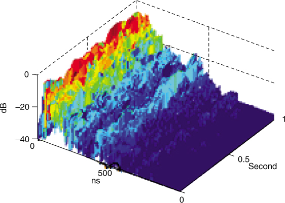
Figure 4.51 Delay Doppler spectrum illustrating the resolution of multipath components in range and in Doppler shift.
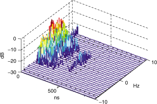
4.12.3 Practical Consideration of Detection Methods of FMCW Signals
Sections 4.12.1 and 4.12.2 gave two possible detectors for the chirp signal. The two techniques provide similar information with regard to the range or time delay and Doppler shift. While the matched filter detector gives the multipath structure in real time as the output consists of the time compressed signal, the heterodyne detector requires a spectrum analyzer to perform the same function. Since the matched filter compresses the signal in time (Figure 4.46), its bandwidth remains unchanged and hence to acquire the data would require quadrature detectors and high bandwidth digitizers. In contrast, the heterodyne detector compresses the signal in bandwidth and not in time, as seen from Figure 4.49, and thus enables the use of low bandwidth acquisition digitizers where the bandwidth depends on the maximum time delay or the range of the farthest echo, and the sweep rate is given by B/T. The total number of samples to be stored using a heterodyne detector is reduced from the usual 2BT (or 4BT for bandpass sampling) to 2Bτmax, where τmax is the maximum expected time delay. For example, for mobile radio sounding at 1.8 GHz and vehicle speeds up to 100 km/h giving a 166 Hz Doppler bandwidth, using a 100 MHz chirp bandwidth and a 500 Hz WRF would require an 800 kHz lowpass filter with a 1.6 MHz sampling rate for a time delay coverage equal to 16 µs. While this sampling rate may not appear to be excessive using state of the art technology, further reduction in sampling requirements can be achieved using an advanced waveform design, as discussed in Section 4.13.
4.13 Range Doppler Ambiguity of Chirp Signals: Advanced Waveforms
Unlike pulse transmission, if the WRF is inadequate to sample the highest Doppler frequency, an FMCW signal moves the echo to a different range bin by the Doppler shift. That is if the WRF ≤ 2fdmax, the range or time delay information cannot be extracted from measurement of the beat note alone on a single sweep basis. Since the Doppler frequency affects the detected range, this gives rise to an ambiguous range estimation, referred to as the range/Doppler ambiguity. To resolve this ambiguity a number of solutions can be employed:
The linear frequency ranging system consists of a linear frequency modulation section whose duration is chosen to avoid range ambiguity, followed by a CW transmission as illustrated in Figure 4.52, which provides an independent measure of Doppler shift. By measuring the instantaneous difference between the frequency of the received echoes and the frequency of the transmitter during the modulation part an algebraic sum of the target Doppler and range is obtained. The target's range is subsequently determined from the difference frequency between the modulated section and the CW section. This type of waveform is useful for a discrete target while for distributed targets such as sea echoes it is difficult to identify the target, which corresponds to the Doppler shift measured during the second half.
Figure 4.52 Linear frequency ranging waveform followed by CW transmission.
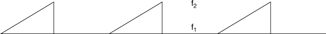
The triangular modulation consists of two linear frequency modulation sections with positive and negative slopes as in Figure 4.53. In this case the difference frequency between the transmitted signal and the received signal consists of the algebraic sum and difference of the range and Doppler frequencies. Subsequently, the target's range and Doppler frequency can be determined from the sum and difference of the estimated frequencies during the up and down sweeps respectively. However, this technique also suffers from the same disadvantage as the linear frequency ranging technique with regard to distributed targets [34].
Figure 4.53 Triangular waveform.
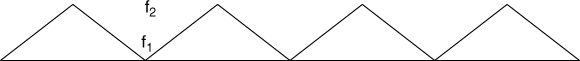
4.13.1 Three-Cell Structure
The three-cell structure illustrated in Figure 4.54 transmits three sweeps, each corresponding to a cell [38] where the sweep duration is chosen to cover the time delay of the farthest echo and the phase difference between the three sweeps is used to resolve the Doppler range ambiguity, assuming that the Doppler frequency does not vary over the three-cell structure period. In this structure the first two sweeps have identical start and stop frequencies, whereas the start frequency of the third sweep is offset by Δf, whose value is chosen to cover the highest expected Doppler frequency.
Figure 4.54 Three-cell structure [38]. Source: Poole, A.V.W., (1985), Advanced sounding 1. The FMCW alternative, Radio Sci. 6, pp. 1609–1616. Reproduced in accordance with guidelines from Radio Science.
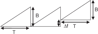
The initial processing of the received signal following the heterodyne detector is similar to the regular FMCW transmission where the FFT is applied to each cell to obtain the in-phase and quadrature components for each multipath component. This gives an estimate of the amplitude, frequency of the beat note and the phase. Since the waveform repetition frequency is insufficient to estimate the Doppler frequency this results in a 2πK phase ambiguity in the Doppler estimate as expressed by:
where ![]() is related to the estimate of the phase in cells 2 and 1,
is related to the estimate of the phase in cells 2 and 1, ![]() respectively, by:
respectively, by:
4.80b ![]()
In [38] an expression for K is derived as:
4.80c ![]()
where ![]() is the instantaneous frequency of the beat note and the expression for the range frequency fR is given by:
is the instantaneous frequency of the beat note and the expression for the range frequency fR is given by:
4.80d ![]()
with
and ![]() is the estimated phase in cell 3:
is the estimated phase in cell 3:
4.80f ![]()
To estimate the Doppler frequency, the frequency offset needs to satisfy the condition:
4.81 ![]()
From Equations (4.78b) and (4.80a)-(4.80e) the Doppler resolution and the range resolution with a three-cell structure is equal to 1/T Hz and (B/T)/Δf Hz respectively. If higher Doppler rates are likely to occur the value of Δf can be reduced at the expense of range resolution. In contrast, the Doppler resolution with regular sounding depends on the number of consecutive sweeps N that are used to extract the Doppler frequency, that is 1/(NT) Hz. The Doppler resolution for the three-cell structure system is limited by the error in the measurement of the phase that depends on the signal to noise ratio. High transmitter powers are needed to improve the system's performance.
In addition to resolving the range Doppler ambiguity, the three-cell structure has the additional advantage of being able to accommodate high Doppler shifts with a relatively low sweep rate, which also reduces the cut-off frequency of the lowpass filter and the corresponding sampling rate for data acquisition. Table 4.8 gives two examples in mobile radio sounding with a 100 MHz bandwidth and a 40 MHz bandwidth. Assuming a 30 Hz Doppler shift with a 100 MHz bandwidth and a 166 Hz Doppler shift with a 40 MHz bandwidth, the corresponding frequency offsets are 5 and 3.9 MHz respectively. This in turn requires only a 4 Hz or 40 Hz WRF instead of the 90 Hz or 500 Hz WRF assuming three times sampling of the maximum Doppler shift. For a 16 µs time delay window the cut-off of the lowpass filter is seen to be reduced considerably. This advantage is particularly important for ultra-wideband applications where bandwidth compression would be highly desirable.
Table 4.8 Comparison of waveform parameters between regular FMCW and the three-cell structure
| Indoor measurements | Regular sounding | 3-Cell structure |
| Bandwidth | 100 MHz (40 MHz) | 100 MHz (40 MHz) |
| fd | 30 Hz (166 Hz) | 30 Hz (166 Hz) |
| Δf | 0 | 5 MHz |
| 0 | (3.9 MHz) | |
| Waveform repetition rate | 90 Hz | 4 Hz |
| (500 Hz) | (40 Hz) | |
| Lowpass filter bandwidth | 4.5 kHz | 200 Hz |
| (320 kHz) | (25.6 kHz) |
4.13.2 Multiple WRF Structure
In this technique multiple blocks of regular FMCW signals with different WRF are transmitted during a single target illumination as shown in Figure 4.55, such that WRF3 > WRF2 > WRF1> [39, 40]. The duration of each WRF and the number of sweeps during each WRF are chosen adequately to resolve range ambiguities and to achieve the required Doppler resolution respectively. The Doppler shifts of targets are estimated sequentially during each block. Since the waveform repetition frequencies of the multiple waveforms are different, aliasing can cause the estimated Doppler shifts to be different during each WRF. The Chinese remainder theorem can be utilized to calculate the true Doppler shift where the maximum unambiguous Doppler range is limited by the least common multiple (LCM) of the selected WRFs [41, 42]. By this technique it is possible to increase the Doppler coverage by increasing the number of waveforms. For the example of HF sea state radar applications three waveforms are adequate to extend the unambiguous Doppler shift higher than 70 Hz to eliminate the ambiguity caused by flying aircraft, which fold over the wanted component from the sea scatter. For example, for 5, 6 and 7 Hz WRF the maximum Doppler coverage is ± 105 Hz (5 × 6 × 7)/2. A suitable two-stage algorithm is then applied to these ambiguous Doppler shifts to deduce the ‘true’ one.
Figure 4.55 Three-WRF structure [39].
Source: Musa, M., and Salous, S. Evaluation of multiple WRF-HF FMCW radar waveform, (2000), Eighth International Conference on HF Radio Systems and Techniques. IEE Conf. Publ. No. 474, pp 207–211. Reproduced with permission of IET.
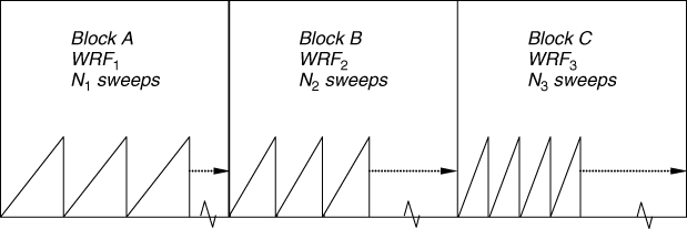
The processing of the multiple WRF signal consists of two stages where in the first stage processing is performed on each block by using the double (FFT) as in a regular FMCW radar. This provides three estimates of range and Doppler, one from each block. The second stage is to map these three estimates into a single range/Doppler space. This process needs to take into account several points such as:
Choosing WRFs that cover the range of interest, the following describes Doppler and range extraction from the three estimates.
4.13.3 Target Movement
The total distance moved by the target during the first block is:
where v1 is the velocity of the target in m/s during WRF1, Tw is the duration of each block in seconds and fc is the radar carrier frequency in Hz. The measured range during the second and third blocks Rm2, Rm3 includes the contribution of both the Doppler shift and the total range crossed during the other two blocks as given in Equations (4.82) and (4.83a).
4.83b ![]()
4.13.4 Doppler Shift Estimation
Fixed WRF radar is capable of resolving Doppler frequencies within ± WRFi/2; that is only fractions of the WRF can be detected and any phase changes greater than 2π radians or equivalently an integer number of cycles cannot be detected. Thus in each WRF we can express the Doppler shift in terms of an integer number ni and a fractional estimate xi where –WRFi/2 ≤ xi ≤ WRFi/2. Thus for the three-WRF example, the Doppler shift of the target in each block can be expressed as [40]:
Solving Equation (4.84) for n3, we get:
In the region where n2 = n3 and n1 = n3, Equations (4.85a) and (4.85b) may be written as:
From the measurements, we have the estimates of x1, x2 and x3, which when used in Equations (4.86a) and (4.86b) give two values of n3. Usually these two values will not be equal. Since, at true Doppler shift, the values of n3 from the two equations should be equal, we increment/decrement n3 by Δn3,2, which is equal to WRF2/(WRF3 − WRF2) and n3 by Δn3,1, which is equal to WRF1/(WRF3 − WRF1) until the new values of n3 and ![]() become equal. As an example, if a target has an ambiguous Doppler shift in the three WRFs equal to x1,2,3 = 2, −2, 3 Hz, using Equations (4.86a) and (4.86b) gives the initial value of n3 = −5 and
become equal. As an example, if a target has an ambiguous Doppler shift in the three WRFs equal to x1,2,3 = 2, −2, 3 Hz, using Equations (4.86a) and (4.86b) gives the initial value of n3 = −5 and ![]() = −0.5 for WRFs of 5, 6 and 7 Hz. By adding (or subtracting) multiples of Δn3,2 (multiples of 6) to −5 and multiples of Δn3,1 (multiples of 2.5) to −0.5 both n3 and
= −0.5 for WRFs of 5, 6 and 7 Hz. By adding (or subtracting) multiples of Δn3,2 (multiples of 6) to −5 and multiples of Δn3,1 (multiples of 2.5) to −0.5 both n3 and ![]() will be equal at n3 = 7 and hence the true Doppler shift of this target is n3WRF3 + x3 = 49 + 3 = 52 Hz.
will be equal at n3 = 7 and hence the true Doppler shift of this target is n3WRF3 + x3 = 49 + 3 = 52 Hz.
Once the Doppler shift is estimated, it can be decoupled from the range since the detected frequency from the spectral analysis has two components, fR + fd. Subsequently an extended range/Doppler diagram can be constructed. An example of such an application is shown in Figure 4.56 where a target with an 8 Hz Doppler shift is detected from a WRF of 5, 6 and 7 Hz with a maximum Doppler coverage of 2.5, 3 and 3.5 Hz per block.
Figure 4.56 Two targets, one with low unambiguous Doppler and a second with ambiguous Doppler shift (a–c) after the double FFT in each block and (d) after decoupling the range Doppler ambiguity.
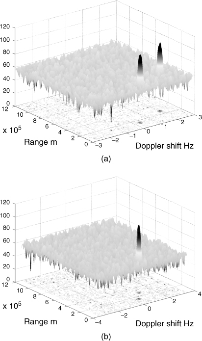
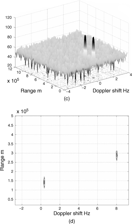
4.14 Architectures of Chirp Sounders
The transmitter of an FMCW radar or sounder consists of a frequency generator capable of frequency sweeping with the appropriate time bandwidth product, locked to a highly stable reference, and a power amplifier as in the block diagram of Figure 4.57a. The receiver can be implemented either with a matched filter detector with quadrature channels or with the heterodyne detector, which provides the bandwidth compression advantage over the matched filter realization. Figure 4.57b displays a block diagram of the heterodyne detector architecture, which requires a locally generated phase coherent replica of the transmitted sweep. To achieve phase coherence, the sweep generator either has to generate an integer number of cycles for each sweep such that the phase always starts with the same initial phase or that the phase is reset at the start of the sweep to the same phase, as illustrated in Figure 4.58. This generally leads to phase discontinuity at the start of the sweep of the generated chirp signal but it ensures phase coherence between the transmitter and receiver.
Figure 4.57 Architecture of FMCW sounder: (a) transmitter and (b) receiver.
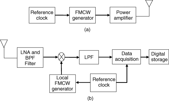
Figure 4.58 Generated quadrature chirp signal with phase reset at the start of the frequency sweep.
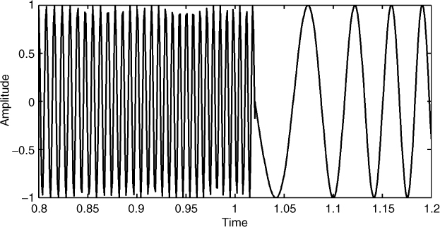
Chirp signals can be generated by a number of techniques, as illustrated in Figure 4.59 [43]. In the passive technique a surface acoustic wave is used to generate the chirp signal. These techniques tend to be limited to generating only the sweep that the device has been designed to generate and thus do not provide flexibility as the active techniques.
Figure 4.59 Chirp generation methods.
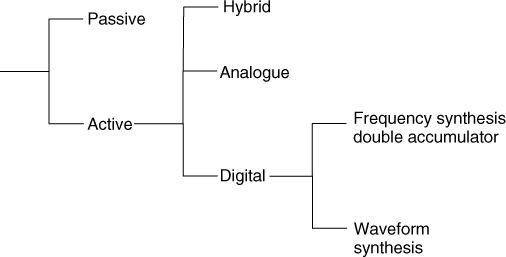
Active techniques can be classified as analogue versus digital where analogue techniques use voltage controlled oscillators (VCOs) programmed with a linear voltage. This technique tends to suffer from the time variability of the characteristics of the VCO and a more accurate technique would be to employ digital techniques that include programming frequency synthesizers in discrete frequency steps. Figure 4.60 shows the architecture of a digital synthesizer, which consists mainly of a phase accumulator to generate the linear steps of the phase of the sinusoid, and a memory look-up table that stores the corresponding amplitude values, which are converted to the analogue domain and then lowpass filtered. The accuracy and dynamic range of a digital synthesizer depend on the phase resolution and the number of bits in the digital to analogue converter. To generate a chirp signal, the frequency of the synthesizer can be programmed in steps as illustrated in Figure 4.60, which can be implemented by an accumulator. Since the linear phase function of the sinusoid can be implemented with a phase accumulator the combination of a frequency accumulator followed by the phase accumulator is referred to as the double accumulator architecture, as shown in Figure 4.61.
Figure 4.60 (a) Architecture using digital frequency synthesis and (b) double accumulator.
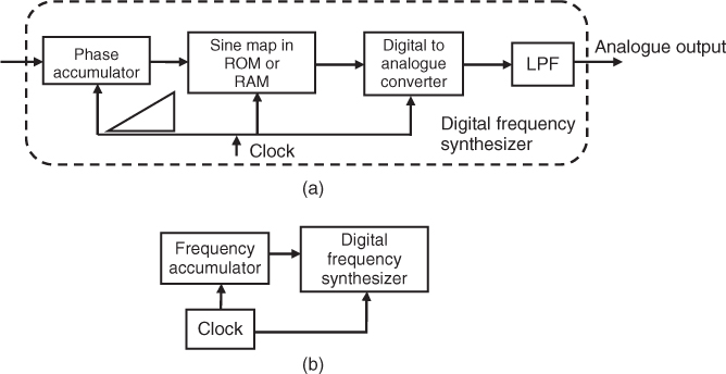
Figure 4.61 Stepped frequency generation of chirp waveforms [44].
Source: Salous, S., Hinostroza, V., Bi-dynamic UHF Channel sounder for indoor measurements, ICAP 2000. Reproduced with permission of IET.

The effect of the stepped generation of the chirp signal is to introduce a phase error which gives rise to sidebands in the compressed chirp signal at (1/Δt) Hz [45] with a level equal to 12.95 + 20 log(1/ΔfΔt) dB below the wanted signal. Other digital techniques use arbitrary waveform generators, which use high speed memory devices to store the samples of a waveform followed by ADCs and lowpass filters. Depending on the clock speed of the digital components the chirp waveform can be generated either at IF or directly at RF. To increase the bandwidth of the generated waveform or to mix up to the required RF, hybrid techniques can be used where the digital IF signal is used as a reference to a PLL with a multiplier or a mixer configuration. In the multiplier PLL configuration, the bandwidth is multiplied by the loop divider N as illustrated in Figure 4.62a. This results in increasing the step size by N,which increases the level of the sidebands in the compressed signal. To use such a configuration, the digital synthesizer has to enable fine frequency resolution. Alternatively, the configuration in Figure 4.62b can be used where the IF signal is mixed by an LO and the signal is then generated by the VCO, which eliminates the need for a BPF, as required by the direct up-conversion method shown in Figure 4.62c. Although the direct up-conversion method requires a filter to eliminate the unwanted sideband, it preserves the frequency step size in the digitally generated chirp signal and also avoids the flyback time due to the time constant of the LPF in the PLL at the start of the sweep when the phase is reset. An alternative is to use a quadrature chirp generator as in Figure 4.62d. While digital generation methods enable accurate generation of the quadrature baseband signals as illustrated in Figure 4.63a, this technique requires balanced quadrature modulation, which can be difficult to achieve with the required rejection of the unwanted sideband, as can be seen from Figure 4.63b.
Figure 4.62 Up-conversion configurations of digitally generated chirp signal [43].
Source: Salous, S., (1992), IF digital generation of FMCW waveforms for wideband channel characterisation. IEE Proc. I., Communications, Speech and Vision, vol. 139, issue 3, pp 281. Reproduced with permission of IET.
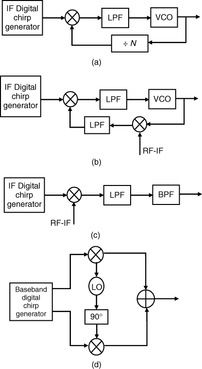
Figure 4.63 Quadrature chirp signal: (a) baseband signal and (b) RF generated chirp signal using quadrature modulator.
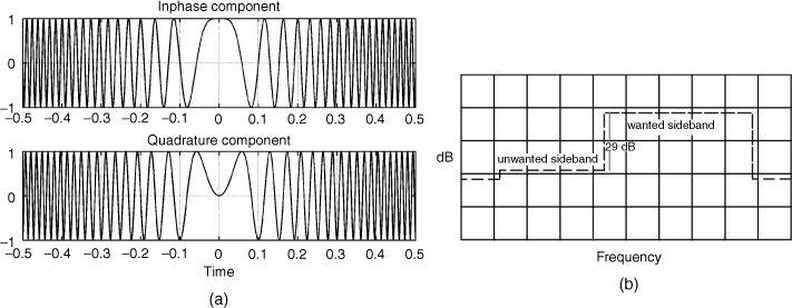
In using digital techniques to generate the chirp signal, the spectrum at the output of the digital synthesizer is that of a chirp signal tapered by the sin x/x function due to the sample and hold effect at the output of the digital to analogue converter. Generally the bandwidth of the generated chirp signal is limited to 40 % of the clock frequency of the digital synthesizer. This has the effect of a gradual decrease of the amplitude of the spectrum as a function of frequency rather than the desired flat spectrum. This slope generally does not affect the compression of the chirp signal. However, amplitude ripple, which might result from filters and other circuit components, has a more detrimental effect on the compressed signal and leads to unwanted sidelobes, which limit the dynamic range of the sounder. The effect of the sin x/x on the spectrum can be compensated for to obtain a flat spectrum as displayed in Figure 4.64 [46].
Figure 4.64 Spectrum of a digitally generated chirp signal with a compensated output [46].
Source: Salous, S., Hinostroza, V., Wideband indoor frequency agile channel sounder and measurements. IEE Proc. -Microw. Antennas Propag., Vol. 152, No. 6. Reproduced with permission of IET.
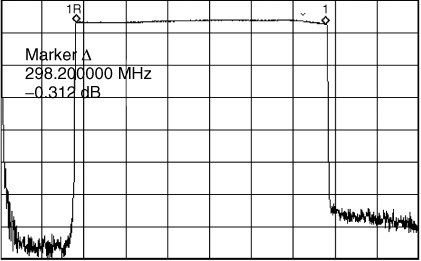
4.15 Monostatic Operation of FMCW Sounder/Radar
Monostatic operation can be used in a number of applications where the transmitter and receiver are co-located. These include vertical sounding of the ionosphere, radar applications such as ground penetrating radar and radio imaging. In narrow pulse sounding, to avoid blocking of the receiver by the high transmitted power, its input can be switched on after the pulse has been transmitted. For FMCW waveforms, listening intervals have to be provided by switching off the transmitter and the receiver at different times, as shown in Figure 4.65, where the transmitted chirp signal is multiplied by g(t) and the receiver's reference is switched using its complement (1 − g(t)), with the resultant modulation being known as a frequency modulated interrupted continuous wave (FMICW).
Figure 4.65 Block diagram of FMICW radar/sounder with associated waveforms.
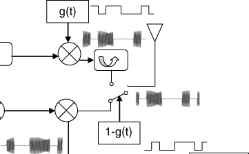
Switching has the following consequences:
4.15.1 Reduction of Effective Mean Received Power
Switching of the transmitted waveform reduces the transmitted power of the signal by an amount that is proportional to the off-time of the FMICW signal with respect to the unswitched FMCW signal. When the delayed received signal is mixed with the reference FMICW signal, the effective input to the lowpass filter is an interrupted CW signal, whose frequency is related to the range or time delay of the target and whose power is related to the time delay and the properties of the switching sequence. From Figure 4.65, the effective input to the lowpass filter s(t) can be represented by:
where T is the duration of the chirp signal and ![]() and
and ![]() are the received and the reference switching sequences respectively. Equation (4.87) represents a gated sinusoid with frequency equal to (B/T)τ and a mean received signal (MRS) equal to the cross correlation between the transmitted and received sequence, as given by [47, 48]:
are the received and the reference switching sequences respectively. Equation (4.87) represents a gated sinusoid with frequency equal to (B/T)τ and a mean received signal (MRS) equal to the cross correlation between the transmitted and received sequence, as given by [47, 48]:

Equation (4.88) shows that the mean received signal varies with the time delay τ or the range of the target with maximum power efficiency is obtained with switching sequences that have a 50 % duty cycle [48]. An alternative to the MRS is to use the mean received power (MRP), in watts, which is equal to the square of the MRS [47].
4.15.2 Spreading of the Spectrum and Interference
When the transmitted chirp signal is switched its spectrum is convolved with that of the switching sequence. This spreads the spectrum of the transmitted signal, which increases interference to other channel users. Similarly, switching of the receiver's sweep increases interference from other channel users as the sidebands of the switching sequence traverse the narrowband interference and shift it to the bandpass of the detector [49]. Figure 4.66 displays the spectrum of a 10 kHz chirp signal prior to and subsequent to switching with the 20 bit sequence shown in Figure 4.67 [50].
Figure 4.66 Spectrum of FMCW and FMICW signal switched with the 20-bit sequence in Figure 4.67.
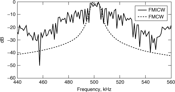
Figure 4.67 Weighted and unweighted edges of a 20-bit sequence.
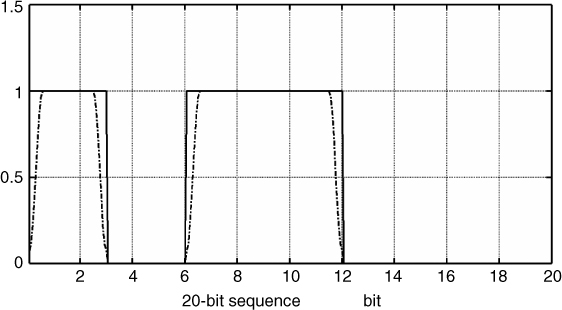
The level of interference is related to the width of the main lobe of the spectrum of the switching sequence, which is governed by the subbit duration τb and the rate of decay of its sidelobes. To reduce interference, the spectrum of the switching sequence can be reduced by weighting the edges of the sequence pulses as illustrated in Figure 4.67.
This, however, has the adverse effect of further reducing the MRP as illustrated in Figure 4.68 for the weighted and unweighted 20 bit sequence. Figure 4.69 displays an example of the spectrum of a 1 kHz FMICW signal prior to and subsequent to weighting, where the sidelobe levels and their rate of decay are seen to be considerably lower than the unweighted spectrum [51].
Figure 4.68 Mean received power versus bit number for the 20-bit sequence with and without weighting with a number of window functions as listed in Table 4.9 [51].
Source: Salous, S., (1997), Weighted sequences for HF FMCW sounding, HF Radio Systems and Techniques, conf. 441, pp 325–329. Reproduced with permission of IET.
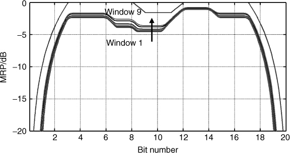
Figure 4.69 Spectrum of weighted (*) and unweighted spectrum of an FMICW signal [51].
Source: Salous, S., (1997), Weighted sequences for HF FMCW sounding, HF Radio Systems and Techniques, conf. 441, pp 325–329. Reproduced with permission of IET.
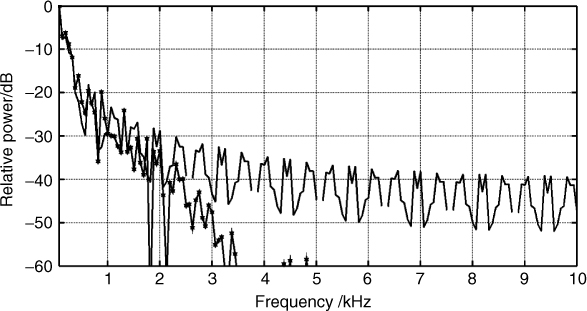
4.15.3 Blind Ranges and Range Ambiguity
‘Blind ranges’ or unseen target ranges can also be analyzed with reference to Equation (4.88). Echoes with time delays, which are multiples of the sequence period Tc, are not ‘seen’ since the product of the received sequence ![]() and the reference sequence
and the reference sequence ![]() is equal to zero as in Figure 4.68. To avoid the occurrence of these ‘blind ranges’, Tc can be chosen to be greater than the maximum expected time delay τmax [48]. Range ambiguities are caused by the spectral lines of the sequence, which occur at multiples of 1/Tc Hz. This can be circumvented by ensuring that the first spectral line of the sequence is outside the frequency range of the wanted echoes. These conditions can be met with sequences whose period satisfies the following relationship:
is equal to zero as in Figure 4.68. To avoid the occurrence of these ‘blind ranges’, Tc can be chosen to be greater than the maximum expected time delay τmax [48]. Range ambiguities are caused by the spectral lines of the sequence, which occur at multiples of 1/Tc Hz. This can be circumvented by ensuring that the first spectral line of the sequence is outside the frequency range of the wanted echoes. These conditions can be met with sequences whose period satisfies the following relationship:
where τmin is the minimum expected time delay. The relationship in Equation (4.89) cannot always be satisfied, where, under such circumstances, sequences with periods comparable to the sweep time that essentially makes the sequence aperiodic can be used [48], thus eliminating the spectral lines of the switching sequence. Alternatively, the sequence period can be made to satisfy the lower limit of Equation (4.89) and blind ranges can be avoided by ‘warbling’ the sequence clock as in the Barry sounder [52].
4.15.4 Selection Criteria for Switching Sequences
The criteria for the selection of sequences are the MRP and interference. While weighting the edges of the sequence reduces the interference, sequences that display a constant MRP as a function of range prior to weighting, such as the M-sequence, have a variable MRP after weighting. The MRP of a 15-bit M-sequence [1 0 1 0 0 0 0 1 1 1 0 1 1 0 0], before and subsequent to weighting, is displayed in Figure 4.70. The edges of the sequence were weighted with the nine different window functions listed in Table 4.9 on a half-bit basis (see example Figure 4.67).
Figure 4.70 Properties of M-sequence: MRP with and without weighting [51].
Source: Salous, S., (1997), Weighted sequences for HF FMCW sounding, HF Radio Systems and Techniques, conf. 441, pp 325–329. Reproduced with permission of IET.
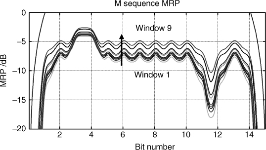
Table 4.9 Window functions and their 6 dB width (columns 1–2), spectrum spreading of chirp signal at specified level down from the peak (columns 3–5) [51]
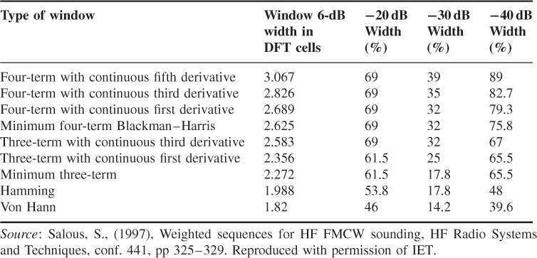
Although the M-sequence displays a significant ‘hole’ in the MRP, long duration M-sequences that satisfy Equation (4.89) can be generated readily with shift registers. Other sequences are the 16 bit Barry sequence (1 1 0 0 0 1 1 1 1 0 0 0 0 0 0 0) [52], used for ionospheric channel sounding and the square wave with 50 % duty cycle used for monostatic radar applications whose MRP are displayed in Figure 4.71.
Figure 4.71 MRP of (a) the 16-bit Barry sequence and (b) 50 % duty cycle square wave [51].
Source: Salous, S., (1997), Weighted sequences for HF FMCW sounding, HF Radio Systems and Techniques, conf. 441, pp 325–329. Reproduced with permission of IET.
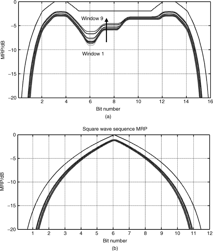
The MRP figures of Figures 4.70 and 4.71a show that the M-sequence reaches its maximum MRP at the end of one subbit, whereas the Barry sequence reaches its maximum MRP at the end of the third subbit. Similar to the M-sequence, the Barry sequence has a 6–8 dB lower sensitivity at the range of bit 6. For channel sounding studies where the relative amplitude of the multipath components is important, it is necessary to equalize the effect of the variable MRP or to use sequences that display constant MRP prior to and subsequent to weighting, such as square waves with duty cycles less than 50 % [53]. This results in a constant MRP that prior to weighting is equal to the square of the duty cycle over a duration equal to the difference between the off-time and the on-time where the maximum MRP is reached at the end of the on-time, as shown in Figure 4.72 for N = 13 bits and a 3 bit on-time.
Figure 4.72 MRP of a square wave with 23 % duty cycle [51].
Source: Salous, S., (1997), Weighted sequences for HF FMCW sounding, HF Radio Systems and Techniques, conf. 441, pp 325–329. Reproduced with permission of IET.
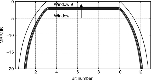
Taking the example of ionospheric sounding, the expected time delay window is approximately equal to 6 ms, which covers a virtual height range of 90–1000 km, with the E-layer being at 0.5 ms. For a 50 kHz/s sweep rate the sequence duration has to be less than 3.33 ms to avoid ambiguities and greater than 6.67 ms to avoid blind ranges. For the detection of the E-layer, suitable bit durations are 0.5 ms for the M-sequence and the Barry sequence and 166 µs for the 20 bit sequence. To compare the amplitude variations of the multipath components for a range of 90–300 km (0.6–2 ms), a square wave with a 0.6 ms on-time and 2.6 ms duration can be used that satisfies the conditions of Equation (4.89). For square wave switching with 50 % duty cycle, a high rate switching rate on the order of 10 kHz to avoid the frequent occurrence of blind ranges can be applied as suggested in [53] whereas for radar applications a square wave with a subbit duration that reaches its maximum at the desirable range can be used.
4.15.5 Considerations for Edge Weighting
A number of factors need to be considered for edge shaping. These include:
4.15.6 Length of the Window
Edge weighting can be applied over the bit or a fraction of the subbit with effects on the MRP and spectral spreading. For the example of the 20 bit sequence in Figure 4.67 using the Von Hann window shaping over both the 1 bit and half-bit, the MRP maximum variations are reduced to 1.3 dB for the half-bit shaping in comparison to 2.75 dB for the 1 bit weighting. However, the corresponding increase in the spread of the spectrum at −60 dB is approximately 160 %, which is more significant than the gain in the MRP.
4.15.7 Window Functions
Similar to spectral analysis (see Section 5.2) different window functions can be used to reduce spectral leakage. Table 4.9 gives the increase in the spectral width of the gated with respect to the ungated chirp signal for three threshold levels ranging from −20 to −40 dB. These are presented for a 10 kHz chirp signal of 60 ms duration switched with the 20 bit sequence with a 166 µs bit period and windowed over 1 bit duration. The increase in the spectral width is seen to be proportional to the 6 dB width of the window as listed in Table 4.9, with the Von Hann (raised cosine) window giving the best suppression of the HF components. This effect is independent of the rate of decay of sidelobes or the level of the peak sidelobe suppression as listed in Table 5.1 (Section 5.2). If the noise floor of the sounder or radar is about −60 dB, the Hamming window gives the best performance in both the MRP and spectral spread.
4.15.8 Interpolation and Quantization
The window function can be implemented either in analogue form or digitally. The advantages of digital shaping include accuracy, flexibility and ease of implementation. The digital realization can be achieved simply by storing the samples of the window function in a read only memory (ROM) lookup table, which can be addressed either by a counter or by an accumulator. The latter permits changing the number of samples of the shaping function. Since the shaping is symmetrical only half the window samples need to be stored. Factors to consider in the digital implementation are the interpolation factor L, which corresponds to the number of samples per bit and the amplitude quantization, q, which determines the number of output bits of the ROM and the size of the digital to analogue converter (DAC). Both L and q affect the spectrum of the generated shaping function, where L determines the aliasing in the spectrum, which decreases as L increases, and q determines the noise floor of the generated spectrum. Figure 4.73 displays the spectrum of the 20 bit sequence, shaped over 1 bit with L values of 64 and 256 and q values of 8 and 12, where the −60 dB level indicates that L = 64 and q = 8 are sufficient.
Figure 4.73 Spectrum of 20 bit sequence with weighting over 1 bit with (a) L = 64, q = 8, (b) L = 64, q = 12, (c) L = 256, q = 8 and (d) L = 256 and q = 12 [51].
Source: Salous, S., (1997), Weighted sequences for HF FMCW sounding, HF Radio Systems and Techniques, conf. 441, pp 325–329. Reproduced with permission of IET.
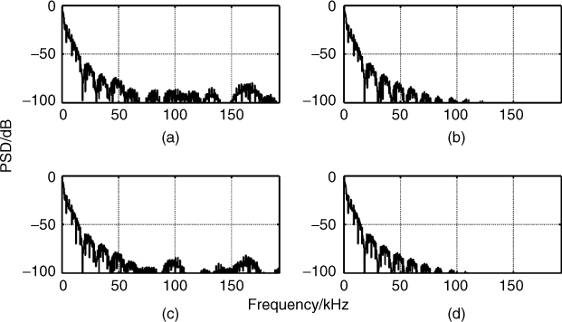
4.16 Single and Multiple Antenna Sounder Architectures
In addition to the classification of static versus dynamic and collocated versus separated transmit and receive units, channel sounders are classified by the number of transmit and receive antennas as single input–single output (SISO), single input–multiple output (SIMO), multiple input–single output (MISO) and multiple input–multiple output (MIMO). The particular architecture used depends on the required information and the application. Numerous MIMO measurements are based on the SISO architecture and very few channel sounders employ a parallel architecture for SIMO, MISO or MIMO measurements. This is due to the complexity and cost involved in designing and building a truly MIMO channel sounder. Hence, the classification used here identifies the architecture via the actual number of hardware channels available in the sounder rather than the type of data that can be extracted from them. MIMO channel sounders are classified into three categories: fully sequential with time division multiplexing (TDM) at both ends of the link, semi-sequential with TDM at the transmitter only with parallel receive channels and full parallel architecture at both the transmitter and at the receiver using a number of orthogonal techniques such as code division multiplexing (CDM) and frequency division multiplexing (FDM). The different types of sounders are discussed and the channel data available from each configuration will be identified in relation to the channel models discussed in Chapter 3.
4.16.1 Single Input Single Output (SISO) Sounders
SISO architectures are the most commonly used in channel sounding. They employ a single transmitter channel and a single receiver channel as displayed in Figure 4.74a. Depending on the waveform used, such architecture yields either narrowband information such as path loss, small-scale fading and location variability or wideband impulse response h(t,τ) measurements, power delay profile and relevant parameters such as average delay, RMS delay spread, time variability, frequency selectivity and Doppler delay functions.
Figure 4.74 Sequential architectures of (a) SISO sounder, (b) MISO sounder, (c) SIMO sounder and (d) MIMO sounder.
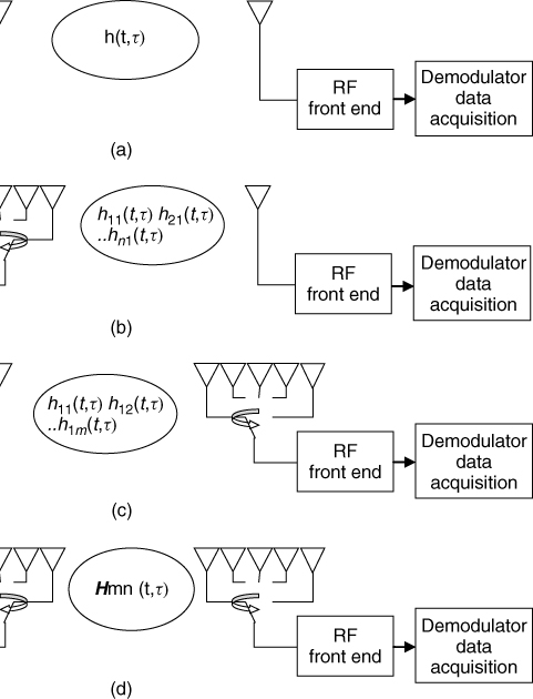
4.16.2 MISO, SIMO and MIMO Measurements with SISO Sounders
As channel models developed to include the angle of arrival θRX and angle of departure θTX, SISO sounders were first modified to transmit or receive from multiple antennas to emulate the MISO or SIMO architecture as in Figure 4.74b,c and subsequently to transmit and receive from multiple antennas for MIMO measurements (Figure 4.74d). Due to the single channels used at both ends of the link these sounders can be classified as TDM or sequential MISO, SIMO or MIMO sounders.
In the sequential SIMO configuration, the sounder can provide single directional angle information whereas in the sequential MIMO configuration, double directional information for both the angle of departure θTX and angle of arrival θRX can be obtained using advanced signal processing algorithms as described in Section 5.11. The switching configuration is used in conjunction with wideband transmissions such as pulse, PRBS or chirp. Consecutive waveforms are transmitted or received sequentially in the MISO or SIMO case, as displayed in Figure 4.75, or transmitted sequentially and received sequentially in the MIMO case, where for each transmitted waveform the receiver switches between all the antennas prior to the next transmitted signal as in Figure 4.76.
Figure 4.75 Sequential transmission/reception in a MISO/SIMO configuration of a SISO sounder.
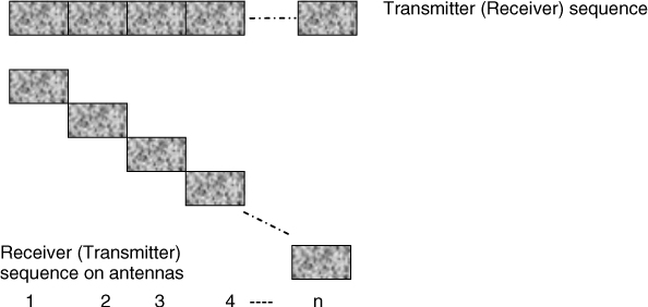
Figure 4.76 Sequence of transmit (receive) signals in sequential MIMO.
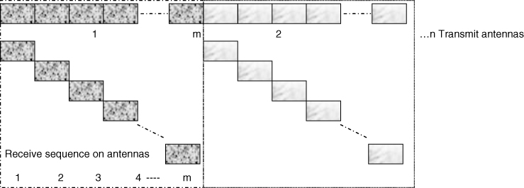
Since the switching in the SIMO configuration is performed at the receiver, the sequence of antennas can be identified. However, this is not the case in the sequential transmission of either the MISO or MIMO configuration where some form of synchronization is required to identify the relevant antenna. One method is to leave a gap in the transmission to identify the start of the transmission sequence. Due to the sequential nature of the measurement, the time required to complete a single measurement depends on the size of the arrays and the duration of the sounding waveform. For n by m arrays the channel sampling rate is reduced by 2 nm. Such measurements assume that the channel is either stationary or quasi-stationary during the time of the measurement, where such measurements tend to be performed in quiet times such as late in the evening.
4.16.3 Semi-Sequential MIMO Sounders
To avoid the switching limitations of SISO sounders in MIMO applications, a semi-sequential configuration can be used where the transmitter is switched between the different antennas with a number of parallel receive channels as shown in Figure 4.77 for the waveform sequence, where an additional time slot is added at the transmitter to identify the end (beginning) of the transmission sequence. Figure 4.78 displays the corresponding architecture for a single transmit channel by m receive channels [54].
Figure 4.77 Semi-sequential MIMO sounder waveforms.
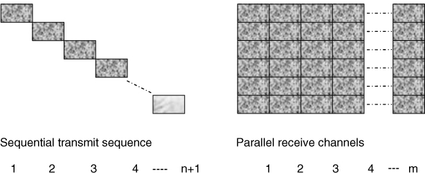
Figure 4.78 Semi-sequential MIMO sounder configuration [54]. Source: S. Salous, P. Filippidis, R. Lewenz, I. Hawking, N. Razavi-Ghods, and M. Abdallah, (2005), Parallel Receiver Channel Sounder for Spatial and MIMO Characterisation of the Mobile Radio Channel. IEE Proceedings on Communication, vol. 152 (6), pp. 912–918. Reproduced with permission of IET.
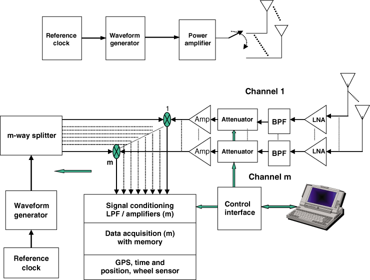
This architecture enables both single frequency band SIMO and MIMO channel measurements as well as multiple frequency band SIMO measurements when used with frequency up- and down-converters [54–56].
4.16.4 Parallel MIMO Sounders
Parallel MIMO sounding transmits and receives simultaneously from all antennas as shown in Figure 4.79. Parallel MIMO sounders achieve orthogonal transmission between the transmitted waveforms using one of three methods:
Figure 4.79 Parallel MIMO sounding.
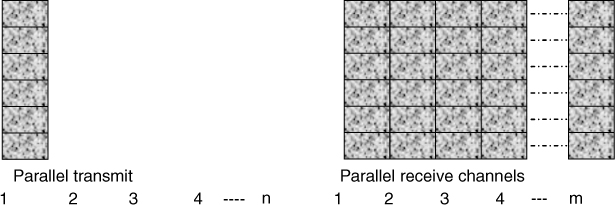
4.16.4.1 Time-Shifted Code
To transmit from several antennas at the same time, the same PRBS sequence can be used where each antenna output is time-shifted with respect to the previous one by a fraction of the length of the sequence. An example of this is the 4 × 8 MIMO sounder which uses a PRBS sequence with a sequence length of 120 data points with 30 points at either end for postprocessing and identification of the sequence [57], as illustrated in Figure 4.80 for four transmit antennas. Each sequence is shifted by a quarter of the length of the previous sequence to generate time-shifted channel responses.
Figure 4.80 Parallel transmission of multiple sequences indicated in the dark blocks and guard periods shown in the light blocks.
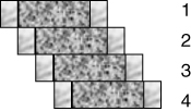
Figure 4.81 displays the correlation properties of a 127 bit PRBS sequence truncated to 120 bits for three multipath components assuming four transmit antennas and reception by a matched filter synchronized to the sequence from the first antenna. Since the sequences are delayed by 30 bits, the correlation peaks from the second antenna appear from bit 30 (2nd cluster) and from the third antenna from bit 60 and from the fourth antenna from bit 90. These offsets are coincident with the time offset between the sequences. The multipath components are seen to be identifiable and each multipath component produces its own side peaks. In the figure the group in the first cluster corresponds to the first transmit antenna. The time delay window of such a sounding waveform is equal to the time delay shift between the sequences that is the number of offset bits divided by the clock of the shift register. For 2.5 MHz bandwidth and 120 bits, this gives (120/4)/(2.5 MHz) = 12 µs time delay window, which is adequate for outdoor mobile radio sounding in the 1.8 GHz band. Figure 4.81 shows an increase in the level of unwanted sidebands and hence a reduction in the overall dynamic range. In the work reported by Yang et al. [57] the dynamic range of the power delay profile appeared to be limited to 18 dB.
Figure 4.81 Correlation properties of time-shifted PRBS sequences used in MIMO sounding.
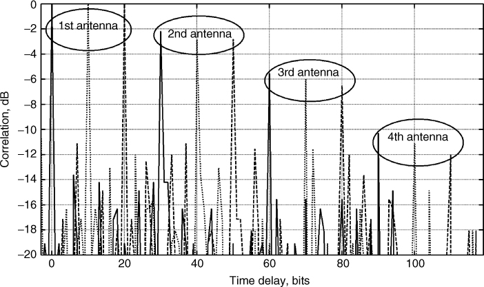
4.16.4.2 Code Division Multiplexing
Parallel transmission can also be achieved by using multiple codes with low cross correlation properties. As shown in Figure 4.37, PRBS sequences of the same length using either the reverse sequence or a different polynomial give a low dynamic range for detection. Alternative quasi-orthogonal sequences designed for code division multiple access techniques, such as Gold codes, and the two families of four-phase sequences, which have been shown to have superior performance to the Gold sequences [58], can be used for MIMO channel sounding. Other codes include the loosely synchronous codes and the Kasami codes, discussed in Section 4.9.
4.16.4.3 Frequency Division Multiplexing
In this technique the different transmit antennas are identified by transmitting either different frequency for all the time or a particular frequency pattern is transmitted cyclically between the different antennas. This can be applied for both the narrowband case and the wideband case. The total offset bandwidth between the different antennas results in a transmission over a higher bandwidth to accommodate the different frequencies.
The simplest FDM scheme is to transmit different CW signals to identify the different antennas [59, 60], which can be identified by spectral analysis. The technique requires that the frequency offset between the carriers is chosen within the coherent bandwidth of the channel to provide the narrowband MIMO channel capacity. For the example of HF propagation [60], 10 Hz carrier offsets are used since the coherent bandwidth of the channel can be on the order of a few kilohertz. The frequency offset can be obtained from programming several digital frequency synthesizers, which can provide accurate phase and frequency programming.
For wideband MIMO applications, frequency division multiplexing can be accomplished in a number of ways depending on the chosen waveform. For example, a PRBS FDM sounder transmits the same PRBS sequence with different carriers for antenna identification at the receiver. Since the spectrum of a PRBS sequence has spectral lines with frequency separation Δf, which is inversely proportional to the period of the sequence, as shown in Figure 4.36b, the frequency offset between the carriers of the PRBS sequences has to be a fraction of Δf. Thus the carrier of the sequence can be frequency offset by dividing Δf/n where n is the number of transmit antennas in an MIMO sounder [61].
Chirp FDM can be achieved by introducing a frequency offset at the beginning of the sweep. The beat notes are then offset in frequency for the different antennas. Bandpass filters that accommodate the required time delay window can be used in the analogue domain as well as in the digital domain. If the signals are separated in the analogue domain it would be possible to use quadrature down-conversion to baseband and quadrature sampling. This, however, is not practical as it requires twice the number of transmit and receive antennas (2*n*m) ADCs. Alternatively, the data are sampled at the highest required sample rate to accommodate the multipath components from all the antennas, which are then separated by digital filtering in the processing. For example, for a radio channel with a 10 µs time delay window, a bandwidth of 30 MHz and 4 ms sweep duration, the required bandwidth per time delay window is 75 kHz. For four transmit antennas, this results in a 300 kHz overall bandwidth, which increases the sampling rate from a minimum of 150 kHz–600 kHz per receive channel with an overall data rate of 2.4 MHz/s.
An alternative to the chirp signal is to transmit the sum of N multiple frequency tones across the desired bandwidth of transmission [62]. The initial phase of each frequency can be chosen in a variety of ways. Using the same initial phase for all the CW tones results in an impulse-like waveform in the time domain and hence the signal has a poor peak power-to-average power ratio. This can be overcome by introducing a random phase between the different tones with the resultant signal in time resembling random noise. To obtain a low peak power-to-average power ratio, it is usual to introduce a quadratic phase function, which results in a time domain signal similar to the chirp waveform. By introducing a frequency offset, parallel MIMO transmission can be achieved with spectral analysis using the discrete Fourier transform (DFT) as shown in Figure 4.82 for two antennas. An example of this technique uses 20 frequencies with 500 kHz separation with 125 kHz offset between antennas [63].
Figure 4.82 Multitone frequency division MIMO sounder waveform.
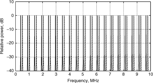
4.17 Ultra-wideband (UWB) Channel Sounders
The origins of UWB go back to the early experiments with the spark-gap generator by Hertz and Marconi. While interest in the 1960s and 1970s was mainly for military applications, recently there has been considerable interest for civilian applications ranging from short range communication to geolocation and breast cancer radio imaging. UWB signals are classified according to either their absolute bandwidth or relative bandwidth. Following the FCC definition [64], a UWB signal either has an absolute bandwidth greater than 1.5 GHz or more regardless of the carrier frequency or has a 25 % fractional bandwidth defined as in the following equation, where the upper frequency fH and the lower frequency fL are the −10 dB points:
4.90 ![]()
UWB waveforms are seen to offer the following advantages:
While UWB systems are expected to have a very low power spectral density below the noise level, various regulations have been introduced that specify frequency bands and power levels. In the United States, the FCC restricted the frequency band between 3.1 GHz and 10.6 GHz for communication systems with a maximum power spectral density equal to −41.3 dBm/MHz for indoor communication. For wall imaging systems and ground penetrating radar the admissible frequency range is either in the 3.1 GHz–10.6 GHz range or below 960 MHz, whereas for through-wall and surveillance systems, the frequency ranges from 1.99 GHz to 10.6 GHz and below 960 MHz are allowed. Vehicular radar systems have frequency ranges between 24 and 29 GHz and around 60 GHz [64].
UWB radar in the 24–29 and 60 GHz bands is governed mainly by line of sight propagation, while other UWB frequency allocations require radio channel measurements to study the frequency dependence of the propagation medium. Due to the high bandwidth requirements and the short range of the proposed applications, radio channel measurements can be performed using standard equipment such as vector network analyzers (VNAs) as illustrated in Figure 4.83 or impulse-like transmissions with high sampling rate oscilloscopes. Custom designed and built PRBS channel sounders for channel measurements and radar applications can also be implemented. In either case one of the main challenges is the design and construction of a suitable wideband antenna and for such measurements the antenna forms an essential part of the radio channel. The VNA provides a simple set-up for such measurements as it is readily available and for UWB applications it provides adequate coverage of range. However, the main shortcoming of the network analyzer is the slow sweep time, which is on the order of 100 ms, which does not enable the measurement of Doppler shift.
Figure 4.83 Network analyzer measurements of radio channels.
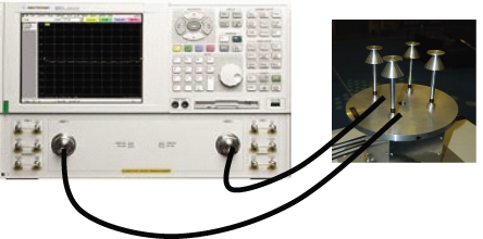
4.18 Sounder Design
The design of a channel sounder requires a set of specifications that determines its parameters such as the choice of a suitable waveform and the overall architecture. The specifications depend on the purpose of the measurements, which can be either for scientific applications and a better understanding of the propagation phenomena or for the design of a specific wireless system. Essential to the design of a channel sounder is the environment to be measured or the medium of transmission: indoor environments for personal wireless networks, outdoor environments for cellular systems, terrestrial radio links for point-to-point or point-to-area microwave radio links, study of skywave propagation via the ionosphere or study of the troposphere for over the sea links. In the case of radar applications, the specifications are related to the application, such as a study of the sea state, car radar, air traffic control, and so on. An important factor is the choice of the frequency band, which can be determined either by the regulators of the spectrum or by the medium of transmission. For example, the ionosphere can support propagation in the HF band but ultra-high frequency (UHF) signals travel through the ionosphere and thus do not provide a communication link. On the other hand, millimetre waves in the 60 GHz band can be used in indoor transmissions and in short range outdoor communication, but do not provide long range coverage. Thus having selected the appropriate carrier frequency and determined the environment to be measured, a possible set of specifications can include the following:
- Time delay resolution of multipath. This refers to the smallest difference in time delay between discernable multipath components. For example, a 10 ns time delay resolution corresponds to a 3 m difference in travel distance that can be distinguished as arriving sequentially.
- Time delay window. This refers to the overall time delay spread of a multipath and the farthest distance that can be measured. The overall time delay window of the channel sounder, however, has to be in excess of the extent of multipath to allow for travel distances away from the transmitter. For example, if the multipath components are expected to extend over 500 ns and the distance between the transmitter and receiver corresponds to 600 ns, then the overall time delay window has to be in excess of 1100 ns to ensure that the movement of the multipath components is still within the observable window. This effect is illustrated in Figure 4.84 in an indoor environment where the transmitter was fixed and the receiver was moved to different locations.
- Doppler coverage. This corresponds to the maximum expected Doppler shift
 , which is equal to
  . This determines the waveform repetition frequency of the sounder, which has to be at least equal to
  . In environments where this condition is not satisfied by the sounder, it is usual to perform the measurements in quiet times when using a VNA or to drive at a lower rate commensurate with the WRF of the sounder.
 - Doppler shift resolution. This corresponds to the smallest Doppler shift that can be measured by the sounder. Theoretically this is proportional to the inverse of the time duration of the observation. Practically this is limited by the phase noise of the frequency sources in the sounder, which broaden the width of the detected Doppler component.
- Synchronization between the transmitter and receiver for accurate measurements. Time synchronization and frequency stability between the transmitter and the receiver is important for accurate measurement of a number of channel parameters including the time delay and Doppler shift. This is usually ensured by using high stability frequency standards. The relative drift between the standards causes each multipath component to appear in a number of range bins during the observation interval. In addition, for accurate Doppler estimation it is usually assumed that the drift between the two frequency standards is less than the resolution cell of the sounder; that is the two sources have not caused a movement of one range bin. This time drift is determined by the stability of the reference frequency sources.
- Stability and phase noise of reference sources. To ensure accurate measurements of the channel characteristics and dynamic operation over long ranges, rubidium standard reference oscillators with low phase noise are usually used at the transmitter and at the receiver.
Figure 4.84 Multipath delay spread as a function of location.
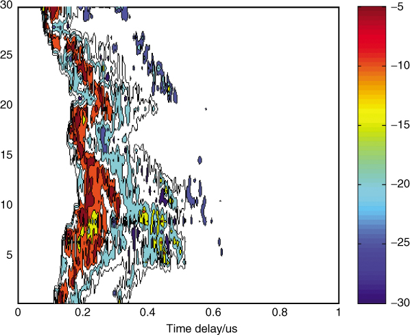
Frequency standards are specified in terms of their Allan variance ![]() , which can be obtained by considering the deviations of the frequency from the ideal reference oscillator, which should have a constant frequency free from time variations, as represented by:
, which can be obtained by considering the deviations of the frequency from the ideal reference oscillator, which should have a constant frequency free from time variations, as represented by:
4.91 ![]()
However, due to the presence of phase noise ![]() , the output is now represented by:
, the output is now represented by:
4.92 ![]()
Taking the derivative of the phase gives the instantaneous frequency as:
Rewriting Equation (4.93) in the following form:
4.94 ![]()
and taking the integral of the kth observation over the observation time τ, the average phase noise can be found from:
4.95 
By taking M measurements each over ![]() seconds and evaluating the average for each time interval, a set of difference values
seconds and evaluating the average for each time interval, a set of difference values ![]() can be found. By taking the ensemble average
can be found. By taking the ensemble average ![]() of the square of the difference, the Allan variance is defined as:
of the square of the difference, the Allan variance is defined as:
4.96 
Similar to the variance and standard deviation, the Allan deviation is obtained from the square root of the Allan variance. Typical values of the Allan variance of rubidium standards are on the order of 2 × 10⁻¹¹ over 1 s, 1 × 10⁻¹¹ over 10 seconds and improve to 2 × 10⁻¹² over 100 seconds [65]. Figure 4.85 gives the square root Allan variance of a rubidium response over time and shows that the variance reduces over a long period of time. The long term stability can be enhanced by locking the standard to the GPS whereas the short term stability is seen to deteriorate initially and then to improve over time to exceed that of the free-running rubidium [65].
Figure 4.85 Square root Allan variance as a function of time [65].
Source: Frequency Standards, PRS10–Rubidium frequency standard with low phase noise, http://www.thinksrs.com/downloads/PDFs/Catalog/PRS10c.pdf Reproduced with permission.
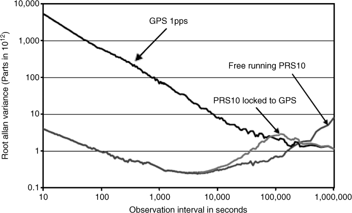
The single-side band phase noise spectrum L(f) in dBc/Hz of an oscillator can be measured using spectrum analyzers. To relate the measured spectrum to the different noise processes that make up the phase noise ![]() , use can be made of their frequency properties. Noise processes that make up phase noise of a signal source are divided into five categories based on their frequency or time dependence. These are classified as: random walk frequency, flicker frequency, white frequency, flicker phase and white phase. Table 4.10 gives the time and frequency dependence properties of the different sources of noise that can be superimposed on the measured phase noise as illustrated in Figure 4.86 [66].
, use can be made of their frequency properties. Noise processes that make up phase noise of a signal source are divided into five categories based on their frequency or time dependence. These are classified as: random walk frequency, flicker frequency, white frequency, flicker phase and white phase. Table 4.10 gives the time and frequency dependence properties of the different sources of noise that can be superimposed on the measured phase noise as illustrated in Figure 4.86 [66].
Table 4.10 Frequency and time dependence of noise processes in frequency sources [66]
| Noise process | Frequency dependence | Time dependence |
| Random walk frequency | f−4 | |
| Flicker frequency | f−3 | |
| White frequency | f−2 | |
| Flicker phase | f−1 | |
| White phase | f0 |
Source: Time domain oscillator stability measurement Allan variance, http://www2.rohde-schwarz.com/file_11752/1EF69_E1.pdf. Reproduced with permission.
Figure 4.86 Phase noise as measured with a spectrum analyzer and the superimposed five slopes from Table 4.10 [65].
Source: Frequency Standards, PRS10–Rubidium frequency standard with low phase noise, http://www.thinksrs.com/downloads/PDFs/Catalog/PRS10c.pdf Reproduced with permission.

In channel sounding, the effect of frequency variations between the transmitter and receiver is a movement with time of the position of the multipath components from their detected time delay, which results in smearing of the response of the channel. The tolerable frequency drift is thus determined by the resolution of the sounder and the overall duration of the measurement. For example, for a 16.67 ns time delay resolution and a 30 minute acquisition interval of data the theoretical stability required from the standards is equal to 1 × 10¹¹, whereas for a 10 ns time delay resolution and 30 minutes of measurements, the drift in the frequency standards has to be on the order of 5.5 × 10⁻¹². Thus the higher the time delay resolution of the sounder the shorter is the time of the measurement. For separate rubidium standards at the transmitter and at the receiver, the relative drift of the sources is important as the multipath components move between time delay bins in a random manner, as illustrated in Figure 4.87a,b for a line of sight measurement where the time delay of the first arriving component moved closer and then farther away despite the movement of the receiver away from the transmitter. This relative time drift has the consequence of inaccurate estimate of the range or absolute time delay. In these circumstances using a controlled trolley or vehicle with an accurate distance measurement would aid in resolving the inaccuracy due to the relative time drift. If this drift is significant, it is possible to lose synchronization between the transmitter and the receiver as the received signal moves outside the time delay window of the sounder. Other effects of phase noise include increasing the estimated MIMO capacity, error in the estimated channel angular parameters such as the direction of arrival (DOA) and direction of departure (DOD), and limiting the resolution of Doppler shift.
- Location information, such as geographic location and distance travelled during the measurement to study path loss or variations of the multipath structure versus range. This can be achieved by a combination of wheel sensor and GPS data.
- Dynamic operation. This enables separate transmitter and receiver mobility by using a separate transmitter and receiver. Restricted mobility arises when using VNAs.
- Multiple antennas. Multiple antenna configurations provide both directional information and channel capacity of MIMO systems.
- Bandwidth compression. This is particularly needed for sounders that employ wideband measurements and enable the use of low data acquisition units.
Figure 4.87 (a) Multipath structure versus location number (range) [46] and (b) time delay of first arriving echo versus location number (range).
Source: Salous, S., Hinostroza, V., Wideband indoor frequency agile channel sounder and measurements. IEE Proc. -Microw. Antennas Propag., Vol. 152, No. 6. Reproduced with permission of IET.
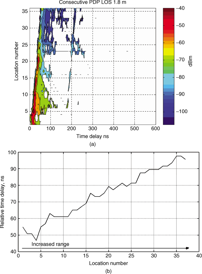
To illustrate the application of these requirements we will consider herein examples in specific environments.
4.18.1 Sounder for Indoor Radio Channels in the UHF Band
To measure an indoor radio environment the channel sounder requires a time delay resolution on the order of 3 ns, which corresponds to a 1 m range resolution that is commensurate with the dimensions of most rooms, office buildings and corridors. Due to the limited dimensions, this also impacts on the maximum time delay window, which is a few hundred ns. Allowing for the movement of the receiver, a time delay window between 500 ns and 1000 ns is sufficient.
Taking into account the limited mobility in an indoor environment, which is unlikely to exceed 2 m/s, the corresponding maximum expected Doppler shift is 13 Hz at 2 GHz. These two parameters determine the bandwidth of the transmitted signal in a chirp sounder or the bit duration in a PRBS sounder and the WRF. For this example, a 300 MHz bandwidth or 3 ns bit duration is sufficient for the time delay resolution, with a WRF of 39 Hz (three times the expected maximum Doppler shift), which provides a time delay window equal to 25 ms and is far in excess of the required time delay window. Due to the high bandwidth of transmission, bandwidth compression would be desirable and for a 300 MHz chirp signal repeated at 100 Hz using a heterodyne detector would require an LPF with a 30 kHz cut-off to cover a 1 µs time delay window. Multiple antenna measurements can be enabled via time delayed or frequency offset chirp signals on the order of 50 kHz between sweeps for parallel transmission. Multiple antenna measurements can also be enabled through TDM and semi-sequential operation. For 8 × 8 measurements, a semi-sequential sounder and a TDM sounder would require a repetition rate equal to 8 WRFSISO = 312 Hz and 64 WRFSISO = 2496 Hz respectively.
4.18.2 Sounder for UHF Frequency Division Duplex Links for Outdoor Radio Channels
For outdoor environments, the time delay window is on the order of 16 µs in dense urban environments and can extend to 40 µs in hilly terrain. In addition to longer time delay windows, outdoor environments require a higher Doppler coverage depending on whether the application is vehicular or pedestrian. For vehicular users, at 2 GHz in inner city environments with maximum speed limits of 40 miles per hour (17.7 m/s) the Doppler coverage is 118 Hz with a corresponding Nyquist sampling rate of 236 Hz. However, outdoor environments have lower requirements in time delay resolution. Taking the example of third generation (3 G) mobile radio systems, dual-band architecture enables the simultaneous measurements of the uplink and downlink bands. Since 3 G systems have been allocated 60 MHz of bandwidth for each band that is separated by 190 MHz, the architecture in Figure 4.88 measures the time-variant frequency characteristics of both bands.
Figure 4.88 Block diagram of dual-band radio channel sounder [68].
Source: Salous, S., Gokalp, H., Dual frequency division duplex sounder for UMTS frequency division duplex channels. IEE Proc. Commun. Vol. 149, No. 2, April 2002, pp 117–122. Reproduced with permission of IET.
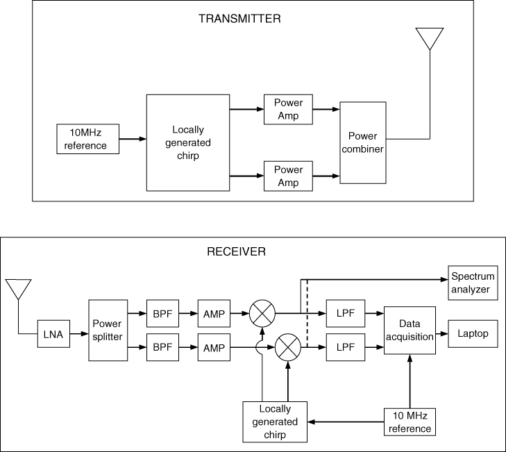
4.18.3 Sounder for Multiple Frequency Links for Outdoor Radio Channels
The dual frequency band can be extended to multiple frequency measurements as illustrated in Figure 4.89. Using up- and down-converters from a suitable IF with a multiple channel receiver, the sounder can measure the multiple frequency bands simultaneously [54]. This technique reduces the time of measurement considerably and enables an accurate comparison of the frequency selectivity of the different frequency bands.
Figure 4.89 Parallel up and down converters for higher frequency bands using a sounder operating at a high IF [56].
Source: Salous, S. Feeney, S.M. Khokhar K. and Lewenz, R., (2008), Measurements of radio channels and BER estimation of IEEE802.16 standard in semi-rural environment at three frequencies in the 2–6 GHz frequency band, IET Communications, vol. 2, No. 7, pp 878–885. Reproduced with permission of IET.
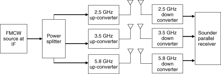
4.19 Performance Tests of a Channel Sounder and Calibration
In radio channel measurements an antenna array can be used in conjunction with a radio channel sounder, which can have any of the architectures described in this chapter. In this section we address the calibration issues associated with the channel sounder in the absence of antennas, that is where only cables connect the transmitter(s) output to the receiver(s) input. This type of calibration is referred to as back-to-back calibration and it consists of evaluating the following:
For a fully sequential time division multiplexing channel sounder, there is a single transmitter and a single receiver and hence the calibration requirements are much reduced in comparison to the fully parallel sounder or the semi-sequential sounder. For a multiple receive sounder, calibration of the different channels is necessary. Here we discuss calibration of a dual-band sounder with multiple receive channels as it has higher requirements than the SISO architecture.
4.19.1 Ambiguity Function
The basic function that determines the choice of a channel sounder or radar waveform is the ambiguity function ![]() defined in Equation (4.29) as the Fourier transform with respect to the Doppler shift variable of the complex baseband signal with its complex conjugate. Thus the main performance test of a channel sounder can be obtained from a back-to-back test where the transmitter is connected to the receiver via a cable as illustrated in Figure 4.90 for an SISO channel sounder and then estimating the ambiguity function.
defined in Equation (4.29) as the Fourier transform with respect to the Doppler shift variable of the complex baseband signal with its complex conjugate. Thus the main performance test of a channel sounder can be obtained from a back-to-back test where the transmitter is connected to the receiver via a cable as illustrated in Figure 4.90 for an SISO channel sounder and then estimating the ambiguity function.
Figure 4.90 Back-to-back test of single input–single output channel sounder.
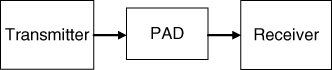
For a dual-band sounder it is necessary to ensure that the two bands do not have any cross products through adequate filtering and individual amplification as shown in Figure 4.91. For an eight channel receiver sounder the ambiguity function is estimated by connecting the sounder as shown in Figure 4.92 where the reference signal is split into eight ways to be fed into the eight channel receiver in parallel and the test includes all the components in the sounder such as the power amplifiers to verify the overall performance. Attenuators are included in the test to bring the signal level below the maximum allowable RF input level to ensure that the system is operating in the linear range. The data are then acquired and processed to obtain the ambiguity function. For a 60 MHz bandwidth this gives an ideal 16.67 ns time delay resolution and, for 1 second of data acquisition, 1 Hz Doppler resolution.
Figure 4.91 (a) Transmitter [54]. Source: S. Salous, P. Filippidis, R. Lewenz, I. Hawking, N. Razavi-Ghods, and M. Abdallah, (2005), Parallel Receiver Channel Sounder for Spatial and MIMO Characterisation of the Mobile Radio Channel. IEE Proceedings on Communication, vol. 152 (6), pp. 912–918. Reproduced with permission of IET. (b) Receiver configuration of dual-band SIMO channel sounder [55].
Source: Razavi-Ghods, N., and Salous S., (2009), Wideband MIMO channel characterization in TV studios and Radio Sci., 44, RS5015, doi:10.1029/2008RS004095. Reproduced in accordance with guidelines from Radio Science.
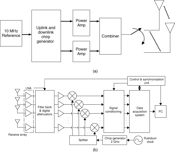
Figure 4.92 Back-to-back test configuration for dual-band SMIO channel sounder [54].
Source: S. Salous, P. Filippidis, R. Lewenz, I. Hawking, N. Razavi-Ghods, and M. Abdallah, (2005), Parallel Receiver Channel Sounder for Spatial and MIMO Characterisation of the Mobile Radio Channel. IEE Proceedings on Communication, vol. 152 (6), pp. 912–918. Reproduced with permission of IET.
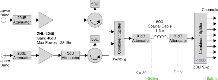
Figure 4.93a and b shows the ambiguity function obtained for both the uplink (1920–1980 MHz) and downlink (2110–2170 MHz). Similarly, as in the SISO case, the time delay and Doppler resolutions can be estimated from the zoomed-in section on the peak of the ambiguity function as displayed in Figure 4.93c and d for the uplink and downlink. Taking the 5 dB contour, we can see that the time delay resolution is approximately equal to 18 ns and ∼1 Hz in the Doppler domain. For a multichannel receiver, it is necessary to obtain similar performance across all the receiver channels.
Figure 4.93 Ambiguity function for the uplink and downlink (a,b) across the entire time delay Doppler shift domain and (c,d) zoomed in section on the peak with 5 dB contours.
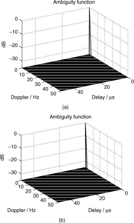
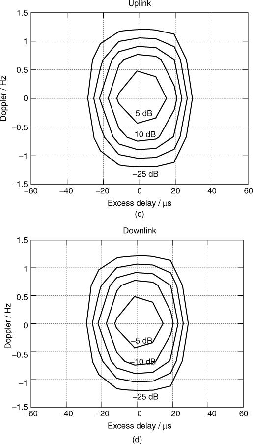
4.19.2 Linearity Test
In a pulse compression sounder, the received multipath components are added together as they arrive at the receiver. This can limit the dynamic range of the sounder and give rise to intermodulation products between the components. To verify the linearity of the receiver, the back-to-back test can be conducted by emulating two paths of comparable amplitude as illustrated in Figure 4.94a for an SISO channel sounder where the output of the transmitter is split into two ways, with one output attenuated and the second output passing through a long cable to generate a second delayed component. The two are then combined at the receiver and the output of the sounder is measured for time delay resolution and for linearity. Figure 4.94b shows the corresponding set-up for a multiple receive channel sounder. Figure 4.95a gives the output from such a test for the universal mobile telecommunication system (UMTS) 60 MHz sounder for the eight receive channels where no other components are detected in the time delay window of the measurement. If the sounder has multiple frequency bands then the linearity test has to be conducted across the different frequency bands, as shown in Figure 4.95b for a dual-band UMTS sounder.
Figure 4.94 Set-up for the linearity test for (a) SISO channel sounder and (b) SIMO channel sounder [54].
Source: S. Salous, P. Filippidis, R. Lewenz, I. Hawking, N. Razavi-Ghods, and M. Abdallah, (2005), Parallel Receiver Channel Sounder for Spatial and MIMO Characterisation of the Mobile Radio Channel. IEE Proceedings on Communication, vol. 152 (6), pp. 912–918. Reproduced with permission of IET.
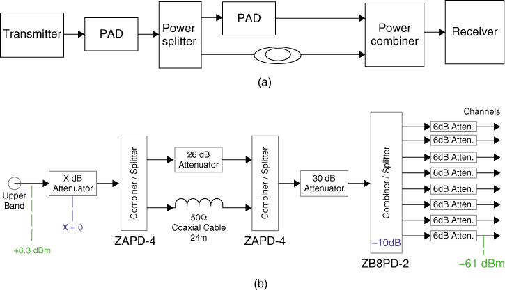
Figure 4.95 Back-to-back test for linearity (a) across eight receive channels and (b) the uplink and downlink bands for one of the eight channels [54].
Source: S. Salous, P. Filippidis, R. Lewenz, I. Hawking, N. Razavi-Ghods, and M. Abdallah, (2005), Parallel Receiver Channel Sounder for Spatial and MIMO Characterisation of the Mobile Radio Channel. IEE Proceedings on Communication, vol. 152 (6), pp. 912–918. Reproduced with permission of IET.
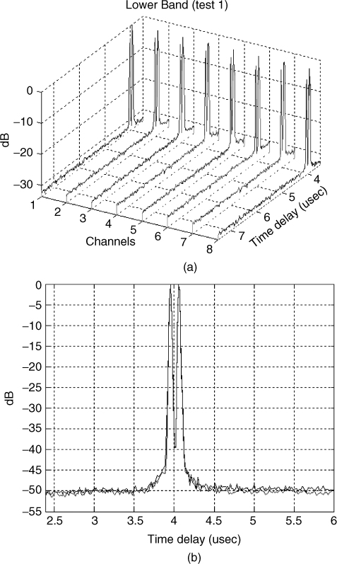
4.19.3 Frequency Response
For studies that require the estimation of the impulse response of the channel as a function of frequency and for frequency selectivity the frequency response of the sounder also needs to be estimated from the back-to-back test and from verification of the spectrum of the transmitted signal. For a PRBS sounder, the envelope of the spectrum is a sin x/x function. For a chirp sounder the spectrum is flat, as illustrated in Figure 4.96, which displays the spectrum of the two UMTS bands at the transmitter and at the receiver. The spectrum is seen to have a flat response, which enables accurate measurements of the frequency domain descriptors.
Figure 4.96 Spectrum of transmit and receive chirp signal [54]. Source: S. Salous, P. Filippidis, R. Lewenz, I. Hawking, N. Razavi-Ghods, and M. Abdallah, (2005), Parallel Receiver Channel Sounder for Spatial and MIMO Characterisation of the Mobile Radio Channel. IEE Proceedings on Communication, vol. 152 (6), pp. 912–918. Reproduced with permission of IET.
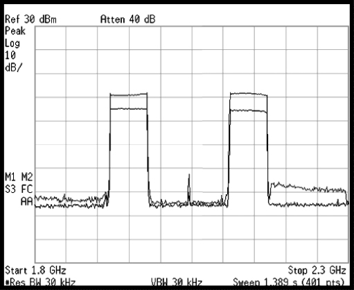
For studies that require the spectrum to be divided into subsections of the measured bandwidth, such as in the case of UMTS measurements where the 60 MHz bandwidth is divided into 5 MHz sections between the users, it is necessary to compare the time delay resolution of the sounder and the amplitude variations across the measured bandwidth. Figure 4.97 gives the time delay resolution obtained across the 12 sections of the 60 MHz bandwidth of the uplink and shows that similar time delay resolution and relative amplitude and dynamic range are obtained across the entire bandwidth [67]. Thus such a channel sounder can be used to measure the radio channel for 5 MHz bandwidth sections to generate comparative frequency measurements. For multiple receive channels the test needs to be repeated for all the channels.
Figure 4.97 Time delay resolution of 5 MHz bandwidth sections [67].
Source: Salous, S., and H. Gokalp, (2007), Medium and large scale characterisation of UMTS allocated frequency division duplex channels, IEEE Transaction on Vehicular Technology, 56(5), pp 2831–2843. Reproduced with permission IEEE.
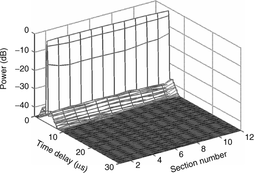
4.19.4 Calibration of Automatic Gain Control
Most sounders have some form of gain adjustment to allow for variations in the RF level of the received signal. Attenuators that can be controlled digitally can be incorporated in the RF section to ensure that the RF mixers are not overloaded to avoid generating unwanted components. Additional signal adjustments are incorporated in a signal conditioning SC unit prior to data acquisition to utilize the full dynamic range of the ADC. In a multichannel receiver, the different channels would have different gain settings and phase shifts, which result from tolerances in the components. Adjustments for the different gains are essential for comparative results between the different channels and for an angle of arrival estimation. The calibration can be performed by applying a known signal level to the receiver as in the back-to-back test and recording the level of the received signal for all the RF and SC settings. This test has to be repeated for each gain setting across all the channels and tabulated.
In operating the sounder each data file is stamped with both the RF attenuation setting and the SC gain and using the tables the gain can be taken into account to obtain the RF signal level if desired using the relationship in:
4.97 ![]()
where GF is a fixed factor due to all other fixed gain/attenuation components in the receive channel from RF up to the SC. For an angle of arrival estimation a calibration file with identical gain settings as the acquired data file can also be recorded from back-to-back tests in order to calibrate the data files. This approach can account for the variations in the sounder performance over time.
4.19.5 Isolation between Multiple Channels
Sounders that employ multiple transmit and multiple receive channels can suffer from signal leakage between channels due to physical proximity of the channels, coupling between cables and imperfect grounds. This can be tested by applying a signal to the input of one channel while terminating the output of another channel with matched impedance and measuring its output. Figure 4.98 shows an example of such a measurement where the level of leakage between channels is at −40 dB down from the wanted signal, which in most channel sounding applications is an acceptable level.
Figure 4.98 Cross talk between channels of a multiple receiver sounder [69].
Source: Filippidis, P, (2002), Multi-Channel Sounder for Directional Measurements. PhD thesis University of Manchester Institute of Science and Technology. Reproduced with permission.
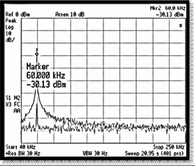
4.19.6 Sensitivity and Dynamic Range
Sensitivity refers to the minimum signal level that can be received with a particular signal to noise ratio. Assuming only thermal noise NT, the theoretical sensitivity of the receiver can be calculated from:
4.98 ![]()
where Tn is temperature in Kelvin and is usually assumed to be 300 K for room temperature, k is Boltzmann's constant and is equal to 1.3806504 × 10⁻²³ J/K, B is the effective receiver noise bandwidth and Nf is the RF noise figure of the receiver.
For a 60 MHz signal bandwidth and an RF noise figure of 10 dB the thermal noise is equal to −86.05 dBm. For a spread spectrum sounder, the processing gain resulting from the compression of the signal enhances the performance of the sounder. For example, for a 60 MHz chirp signal repeated at 250 Hz, the 10 log(BT) is equal to 53.8 dB. Hence the overall theoretical sensitivity is equal to:
![]()
To perform this test, signal levels starting from the minimum signal level, which for this example is −110 dBm, are applied at the receiver input with the back-to-back test configuration and increased in steps of, say, 10 dB. For each signal setting the compressed signal to noise ratio SNRo is measured. An example of such a test is given in Table 4.11, which gives back-to-back test results for an input signal level between −110 dBm and up to −60 dBm. For a minimum SNRo of 30 dB the sensitivity is seen to be close to the theoretical value. The variable attenuator in the RF section of the sounder extends the RF input level from −110 dBm to −60 dBm, giving an overall dynamic range of 30 dB, which can be obtained within 50 dB of RF signal variations.
Table 4.11 Signal to noise ratio at the output as a function of RF level at the input [69]
| RF attenuator (dB) | RF level at the receiver (dBm) | SNRo |
| 0 | −110 | 30 |
| 0 | −100 | 40 |
| 0 | −90 | 50 |
| 0 | −80 | 47 |
| 10 | −80 | 50 |
| 20 | −70 | 50 |
| 30 | −60 | 50 |
Source: Filippidis, P, (2002), Multi-Channel Sounder for Directional Measurements. PhD thesis University of Manchester Institute of Science and Technology. Reproduced with permission.
4.19.7 Effect of Interference on the Dynamic Range
Another related test is to verify the performance of the sounder in the presence of CW interference. Although FMCW sounders have the ability to spread out the interference signal and to compress the wanted signal, the dynamic range of the sounder is reduced as the interfering signal raises the noise floor. Another effect of interference is to block the receiver, thereby reducing its detection capability of small signal levels. The effects of interference on the performance of the sounder can also be studied from back-to-back tests by adding a CW signal to the wanted signal. Figure 4.99 shows a CW interfering signal set at a level 40 dB higher than the level of the wanted signal, which was set at −86 dBm. Apart from a very short duration recovery interval the time domain signal did not reveal any blocking of the receiver. The effect of interference can be studied by processing the data with the required resolution bandwidth. For the example of Figure 4.98 the 90 MHz sweep was divided into 18 MHz sections and 75 % overlap between sections. The resulting power delay profiles versus frequency show that interference raises the noise floor and causes a slight dip of the order of 2 dB in the frequency section where it occurs relative to the neighbouring sections [70].
Figure 4.99 Effect of interference: (a) time domain and (b) power delay profile as a function of frequency [70]. Source: Salous, S. (1999), Measurement of multipath delay statistics over a 72- to 90-MHz bandwidth at 1.8 GHz in two European cities using a chirp sounder, doi:10.1029/1999RS9000014. Radio Science, Vol. 34, No. 4, pp. 797–816. Reproduced in accordance with guidelines from Radio Science.
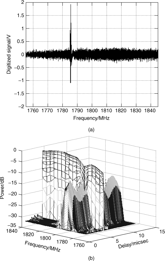
4.19.8 Stability of Frequency Sources
Taking back-to-back measurements at the beginning and at the end of radio channel measurements enables the evaluation of the time drift between the transmitter and the receiver, which can be on average used to correct for the change in time delay to give a more accurate estimate of the absolute time delay of the multipath components. To quantify the relative drift back-to-back tests can be performed on the bench and at the start and end of a measurement and compared with the specification of the frequency standards used in the sounder. In [46] the average drift from such measurements was found to be 3.3 parts in 1011, which is consistent with the specifications of the rubidium and 4 parts in 1012 for the bench measurements.
4.19.9 Temperature Variations
Thermal variations increase thermal noise and result in a reduced dynamic range. In addition, this increases the phase noise in the signal sources and reduces the ability of the sounder to resolve components in the Doppler domain and introduces errors in the estimation of the angle of arrival and angle of departure. To account for temperature variations system measurements need to be performed at regular intervals, in particular for angular information.
4.20 Overall Data Acquisition and Calibration
Data files are normally acquired in small blocks over short intervals on the order of a few seconds. Each acquired data file is stamped with the settings of the sounder including the number of impulse responses, sampling rate/number of samples, location using wheel sensor reading and GPS if used, impulse repetition rate and the SC gains and RF attenuator settings. Due to the time variability of the response of the sounder, calibration files need to be acquired from back-to-back tests for the same settings as the acquired data. The calibration files are then used for compensation. Calibration is particularly critical for sounders with multiple receiver channels as the tolerances on the values of the components and the thermal variations give rise to differences between the different channels. Thus calibration files should be obtained for all the channels simultaneously and each channel is then compensated for its own gain settings. Prior to any processing each data file should be verified for an adequate dynamic range.
References
1. Radar World http://www.radarworld.org/.
2. Parsons, J.D. (2000) The Mobile Radio Propagation Channel, John Wiley & Sons, Ltd, p. 134.
3. Cox, D.C. (1973) 910 MHz urban mobile radio propagation multipath characteristics in New York city. IEEE Trans. Veh. Technol., 22 (4), 104–110.
4. Abdalla, M.M. (2005) Directional antenna array for channel measurement Ssystem. PhD Thesis, Manchester University.
5. Devasirvatham, D.M.J. (1986) Time delay spread and signal level measurements of 850 MHz radio waves in building environments. IEEE Trans. Antennas Propag., 34 (11), 1300–1305.
6. Devasirvatham, D.M.J. (1988) Radio Propagation Studies in a Small City for Universal Portable Communications. IEEE 38th Vehicular Technology Conference, pp. 100–104.
7. Bultitude, R.J.C., Mahmoud, S.A. and Sullivan, W.A. (1989) A comparison of indoor radio propagation characteristics at 910 MHz and 1.75 GHz. IEEE J. Sel. Areas Commun., 7 (1), 20–30.
8. Siddle, D.R., Warrington, E.M. and Gunashekar, S.D. (2007) Signal strength variations at 2 GHz for three sea paths in the British channel islands: observations and statistical analysis. Radio Sci., 42 (RS4019), 15. DOI: 10.1029/2006RS003616.
9. Willis, M.J. and Craig, K.H. (2008) The Correlation of Enhancement and Fading on Terrestrial Point to Point Links, www.ursi.org/proceedings/procGA08/papers/F03p9.pdf.
10. Ibrahim, M.F. and Parsons, J.D. (1983) Signal strength prediction in built up areas. Part 1, median signal strength. Proc. IEE, F, 130 (5), 355–384.
11. Okumura, Y., Ohmori, E., Kawano, T. and Fukuda, K. (1968) Field strength and its variability in VHF and UHF land-mobile radio service. Rev. Electr. Commun., Lab., 16, 825–873.
12. Skolnik, M.I. (1962) Introduction to Radar Systems, McGraw-Hill, New York.
13. Matthews, P.A., Molkar, D. and Rashidzadeh, B. (1985) Measurement, Description and Modelling of the Terrestrial Mobile Radio Channel. Proceedings of 3rd International Conference on Land Mobile Radio, Cambridge, IERE Conference Publication No. 65, pp. 119–125.
14. David, F., Franco, A., Sherman, H. and Shucarage, L. (1969) Correlation measurements on an HF transmission link. IEEE Trans. Commun. Technol. Commun., 17 (2), 245–256.
15. Greenwald, R.A. and Baker, K.B. (1983) Initial studies of small scale F region irregularities at very high latitudes. Radio Sci., 18 (6), 1122–1132.
16. Greenwald, R.A., Baker, K.B., Hutchins, R.A. and Hanuise, C. (1985) An HF phased array radar for studying small scale structure in the high latitude ionosphere. Radio Sci., 20 (1), 63–79.
17. Bajwa, A.S. (1979) Wideband characterisation of UHF mobile radio propagation in urban and suburban areas. PhD Thesis, University of Birmingham.
18. Bailey, R. and Summers, G. (1990) Radio channel characterisation for the digital European cordless telecommunications systems. Br. Telecom Technol., 8 (1), 25–30.
19. Haykin, S. (2007) Introduction to Analogue and Digital Communications, 2nd edn, John Wiley & Sons, Inc.
20. Kasami, T. (1966) Weight Distribution Formula for Some Class of Cyclic Codes. Technical Report No. R-285, University of Illinois.
21. Welch, L. (1974) Lower bounds on the maximum cross correlation of signals. IEEE Trans. Inf. Theory, 20 (3), 397–399.
22. Stanczak, S., Boche, H. and Haardt, M. (2001) Are LAS-codes a miracle? IEEE Globecom, 1, 589–593.
23. Minjae, K., Sunghyun, K., Hyuckjae, L. et al. (2008) Performance Comparison of Some Codes in Code Division Multiplexing Based MIMO Channel Sounder Architecture. ICACT, 10th International Conference on Advanced Communication Technology, pp. 1343–1346.
24. Price, R. and Green, P.E. (1958) A communication technique for multipath channels. Proc. IRE, 46, 555–570.
25. Cullen, P.J., Fannin, P.C. and Molina, A. (1993) Wide-band measurement and analysis techniques for the mobile radio channel. IEEE Trans. Veh. Technol., 42 (4), 589–603.
26. Cox, D.C. (1972) Delay Doppler characteristics of multipath propagation at 910 MHz in a suburban mobile radio environment. IEEE Trans. Antennas Propag., AP20 (5), 625–635.
27. Pirkl, R.J. and Durgin, G.D. (2009) Revisiting the spread spectrum sliding correlator: why filtering matters. IEEE Trans. Wireless Commun., 8 (7), 3454–3457.
28. Vilar, E., Mousley, T.J., Austin, J. et al. (1983) A System to Measure LOS Atmospheric Transmittance at 19 GHz. AGARD Conference Proceedings No. 346, Spatind, Norway.
29. Skaug, R. (1982) An Experiment with Spread Spectrum Modulation on an HF Channel. IEE Conference Publication 206, HF Communication Systems and Techniques, pp. 76–80.
30. Wagner, L.S. and Goldstein, J.A. (1985) High resolution probing of the HF ionospheric skywave channel: F2 layer results. Radio Sci., 20, 287–302.
31. Coll, D.C. and Storey, J.R. (1964) Ionospheric sounding using coded pulse signals. Radio Sci. J. Res. NBS/USNC-URSI, 4.68D (10), 1155–1159.
32. Cook, C.E. and Bernfield, M. (1967) Radar Signals; An Introduction to Theory and Application, Academic Press, New York.
33. Klauder, J., Price, A., Darlington, S. and Albersheim, W. (1960) The theory and design of chirp radars. Bell Syst. Tech. J., 39, 745–808.
34. Skolnik, M. (1989) Radar Handbook, McGraw-Hill, New York.
35. Lundborg, B. and Lundgren, M. (1992) On the spectral shape of chirp sounder signals. J. Atmos. Terr. Phys., 54, 311–321.
36. Salous, S. (1994) Dispersion of chirp pulses by the ionosphere. J. Atmos. Terr. Phys., 56 (8), 979–994.
37. Barrick, D.E. (1973) FMCW Radar Signals and Digital Processing. Technical Report, ERL 283-WPL 26, NOAA.
38. Poole, A.V.W. (1985) Advanced sounding 1. The FMCW alternative. Radio Sci., 6, 1609–1616.
39. Musa, M. and Salous, S. (2000) Evaluation of Multiple WRF-HF FMCW Radar Waveform. 8th International Conference on HF Radio Systems and Techniques, IEE Conference Publication No. 474, pp. 207–211.
40. Musa, M. and Salous, S. (2000) Ambiguity elimination in HF FMCW radar systems. IEE Proc. Radar Sonar Navig., 147 (4), 182–188.
41. Skillman, A.W. (1983) Radar Calculations Using the IT-59 Programming Calculator, Artech House Inc.
42. Allenby, R.B.J.T. and Redfern, E.J. (1992) Introduction to Number Theory with Computing, Edward Arnold, London.
43. Salous, S. (1992) IF digital generation of FMCW waveforms for wideband channel characterisation. IEE Proc. I, Commun. Speech Vision, 139 (3), 281–288.
44. Salous, S. and Hinostroza, V. (2001) Bi-Dynamic UHF Channel Sounder for Indoor Measurements. IEE Conference on Antennas and Propagation ICAP2001, IEE Conference Publication 480, Vol. 2, pp. 583–587.
45. Barry, G. and Fenwick, R. (1965) Extraterrestrial and ionospheric sounding with synthesised sweeps. Hewlett-Packard J., 16, 8–12.
46. Salous, S. and Hinostroza, V. (2005) Wideband indoor frequency agile channel sounder and measurements. IEE Proc. Antennas Propag., 152 (6), 573–580.
47. Ghannad, M.S. (1984) Beamwidth reduction for HF radars. PhD Thesis, submitted to Birmingham University.
48. Poole, A.W. (1979) On the use of pseudorandom codes for chirp radar. IEEE Trans. Antennas Propag., AP-27 (4), 480–485.
49. Shearman, E.D.R. and Unsal, R.R. (1980) Compatibility of High Frequency Radar Remote Sensing with Communications. IEE Conference Publication 188 (Radio Spectrum Conversion Techniques), pp. 103–107.
50. Salous, S. and Nattour, O. (1992) Switching Sequences for Monostatic Pulse Compression Ionospheric Sounders. Proceedings of the 4th Bangor Communications Symposium, Bangor, pp. 346–349.
51. Salous, S. (1997) Weighted Sequences for HF FMCW Sounding. HF Radio Systems and Techniques, Conference, Vol. 441, pp. 325–329.
52. Barry, G.H. (1971) A low power vertical-incidence ionosonde. IEEE Trans. Geosci. Electr., GE-9 (2).
53. Iguchi, T., Umehara, T., Ohno, Y. and Nozaki, K. (1989) Effect of T/R Switching Sequence for an HF Ocean Radar. Proceedings of the International Symposium on Noise and Clutter Rejection in Radars and Imaging Sensors.
54. Salous, S., Filippidis, P., Lewenz, R. et al. (2005) Parallel receiver channel sounder for spatial and MIMO characterisation of the mobile radio channel. IEE Proc. Commun., 152 (6), 912–918.
55. Razavi-Ghods, N. and Salous, S. (2009) Wideband MIMO channel characterisation in TV studios and inside buildings in the 2.2–2.5 GHz frequency band. Radio Sci., 44, 1–13.
56. Salous, S., Feeney, S.M., Khokhar, K. and Lewenz, R. (2008) Measurements of radio channels and BER estimation of IEEE802.16 Standard in semi-rural environment at three frequencies in the 2–6 GHz frequency band. IET Commun., 2 (7), 878–885.
57. Yang, Y., Xu, G. and Ling, H. (2006) An experimental investigation of wideband MIMO channel characteristics based on outdoor non-LOS measurements at 1.8 GHz. IEEE Trans. Antennas Propag., 54 (11), 3274–3284.
58. Bztas, S., Hammons, R. and Kumar, P. (1992) 4-phase sequences with near optimum correlation properties. IEEE Trans. Inf. Theory, 38 (3), 1101–1113.
59. Xu, H., Gans, M.J., Amitay, N. and Valenzuela, R.A. (2001) Experimental verification of MTMR system capacity in controlled propagation environment. Electronics Lett., 37 (15), 936–937.
60. Gunashekar, S.D., Warrington, E.M., Feeney, S.M. et al. (2010) MIMO communications within the HF band using compact antenna arrays. Radio Sci., 45, RS6013. DOI: 10.1029/2010RS004416.
61. Dahman, G.S., Bultitude, R.J.C. and Hafez, H.M. (2009) The use of frequency-orthogonal-pseudo-noise (FOPN) sounding signals for identifying transmissions from different transmit antennas. IEEE Antennas Wireless Propag. Lett., 8, 657–660.
62. Wirnitzer, W., Bruckner, D., Thoma, R.S. et al. (2001) Broadband Vector Channel Sounder for MIMO Channel Measurement. IEE Seminar on MIMO: Communication Systems from Concept to Implementation.
63. Sakaguchi, K., Takada, J. and Araki, K. (2002) A novel architecture for MIMO spatio-temporal channel sounder. ICICE Trans. Electron., E85-C (3), 436–441.
64. Federal Communications Commission FCC (2002) Report 02–48, www.fcc.gov/Bureaus/Engineering…/fcc02048.pdf-United States.
65. Frequency Standards PRS10. Rubidium Frequency Standard with Low Phase Noise, http://www.thinksrs.com/downloads/PDFs/Catalog/PRS10c.pdf.
66. Time Domain Oscillator Stability Measurement Allan Variance, Rhodes and Schwartz, http://www2.rhodes-schwartz.com/file_11752/1EF69_E1.pdf.
67. Salous, S. and Gokalp, H. (2007) Medium- and large-scale characterization of UMTS-allocated frequency division duplex channels. IEEE Trans. Veh. Technol., 56 (5), 2831–2843.
68. Salous, S. and Gokalp, H. (2002) Dual frequency sounder for UMTS frequency division duplex channels. IEE Proc. Commun., 149 (2), 117–122.
69. Filippidis, P. (2002) Multi-channel sounder for directional measurements. PhD Thesis, University of Manchester Institute of Science and Technology.
70. Salous, S. (1999) Measurement of multipath delay statistics over a 72-to 90-MHz bandwidth at 1.8 GHz in two European cities using a chirp sounder. Radio Sci., 34 (4), 797–816. DOI: 10.1029/1999RS900014.