Chapter 5

Data Analysis

Data reduction and analysis is a major aspect of radio channel modelling. Many radio link planning tools and international standards are based on empirical or semi-empirical models extracted from measurements. Hence it is essential that data are acquired at the appropriate rate and accurately analyzed.

In this chapter we study the analysis techniques pertinent to various radio channels. We start with the analysis of a single radio channel measurement (a snapshot) to estimate the impulse response and the frequency response of the channel using basic spectral analysis techniques. We commence with the discrete Fourier transform (DFT) and the effect of the window functions on the estimated channel response. In particular for frequency dispersive channels move on to the more advanced spectral estimation techniques of parametric modelling such as autoregressive (AR), moving average (MA) and autoregressive moving average (ARMA) modelling. Techniques to reduce the effect of interference from measured data will be discussed in particular in relation to ionospheric propagation where the high frequency (HF) spectrum is highly congested.

Another important topic addressed in this chapter is statistical analysis of time and space series. Here, we define and use the RUNS test to determine the stationarity of a process. We then apply it to spatial and time averaging of impulse responses for the estimation of small-scale parameters such as the power delay profile (PDP) and its related parameter, the RMS delay spread. Stochastic modelling of measurements with known cumulative distribution functions (CDFs) and probability density functions (PDFs) is discussed in terms of the goodness of fit. This is followed by the estimation of path loss models as derived from wideband data.

The last part of the chapter addresses high resolution parameter estimation techniques used in double directional analysis such as space-alternating generalized expectation (SAGE), multiple signal classification (MUSIC) and estimation of signal parameters via the rational invariance technique (ESPRIT). Practical aspects of the calibration of antenna arrays used in double directional measurements are presented with examples from a semi-sequential multiple receive sounder. This is followed by a discussion on the estimation of multiple input–multiple output (MIMO) channel capacity.

5.1 Data Validation

Prior to processing and analysis of measured channel parameters it is necessary to ensure that the data are valid and calibrated. A number of issues can occur during data collection. For example, intermittent data collection can happen due to poor connectivity of cables, which can appear as fading in the acquired data. Another source of inappropriate data collection is suboptimum gain calibration in the radio frequency (RF) section of the sounder and in the signal conditioning section. A high signal level in the RF section can give rise to mixer nonlinearity and introduce harmonics or to a low signal level where the received signal is not amplified sufficiently to cover the dynamic range of the receiver. A high signal level in excess of the maximum voltage range covered by the analogue to digital converter (ADC) results in clipping of the data and a low signal level reduces the dynamic range of the response. Another issue in data collection can arise due to lack of synchronization between the transmitter and receiver, which leads to frequency and time drift and possibly the loss of the channel response as it moves outside the time delay window of the sounder. Thus it is necessary to carry out back-to-back measurements prior to data acquisition to obtain reference files to verify the overall performance of the sounder. The gain settings as well as the size of the data file and its parameters need to be stored for later calibration for each data file. Equally prior to processing, the data should be inspected electronically and visually and verified for appropriate dynamic range prior to extraction of channel parameters.

Another issue for data validation is to ensure the appropriate setting of the channel sounder for the particular application in terms of bandwidth, carrier frequency, waveform repetition frequency, distance and time sampling, and power level to reach the intended range of coverage. Appropriate choice of antennas and calibration files should also be obtained and used for interpreting the results of the measurements.

5.2 Spectral Analysis via the Discrete Fourier Transform

In Chapter 3 the radio channel functions were shown to be interrelated via forward and inverse Fourier transform relationships. Also, in Chapter 3 the time series obtained at the output of the heterodyne detector of a frequency modulated continuous waveform (FMCW) sounder was demonstrated to give the delay Doppler function via the double DFT where the first DFT yields the impulse response and the second DFT over the time delay bins gives the Doppler spectrum. Spectral analysis via the inverse DFT is also used to estimate the impulse response from network analyzer measurements.

In DFT processing, the forward transform X[k] of a time domain signal x[n] and the inverse transform are normally given as:

5.1a

5.1b

To relate the result of the forward DFT to the actual voltage level or to the power in the signal, it is necessary to divide the result of Equation (5.1a) by N. Since the spectrum obtained from Equation (5.1a) gives the double-sided spectrum, which for a real time signal exhibits even symmetry in amplitude and odd symmetry in phase, only half the number of points need to be retained. The remaining single-sided spectrum is then multiplied by 2 to represent the spectrum in linear scale or multiplied by 20 log₁₀ to represent the signal in decibels.

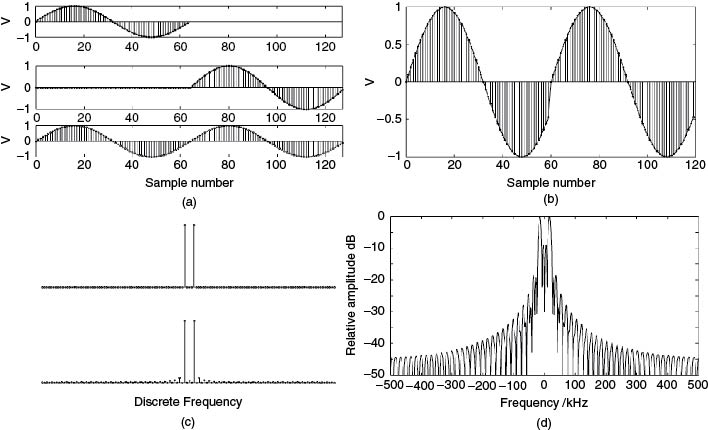
Digital spectral analysis of a finite time duration signal has the effect of periodicity on the signal both in time and in frequency. Since the ideal spectrum of a sinusoid with infinite time duration is an impulse, the finite duration sinusoid can be viewed as an infinite sinusoid multiplied by a rectangular window function. If an integer number of cycles occurs within the duration of the observation interval, then the periodic repetition of the sinusoid appears continuous and the spectrum is that of the ideal impulse function. For example, the time domain signal x[n] given by:

5.2

represents the fundamental component within the 64 points. The value at n = 64 the sinusoid would have is the same value as at n = 0 and the periodic repetition that starts at n = 64 would display a continuous signal as illustrated in Figure 5.1a. If the signal is truncated at the 60th sample, the periodic repetition of the signal in the time domain would appear as in Figure 5.1b, which now has a discontinuity. Assuming a 1 MHz sampling rate, Figure 5.1c and d gives the corresponding spectra for the ideal continuous case of Figure 5.1a and for the discontinuous case of Figure 5.1b respectively.

Figure 5.1 (a) Ideal time domain signal within observation interval, (b) non-ideal time domain signal, (c) spectrum of ideal signal and (d) spectrum of non-ideal signal.

The nonideal spectrum is seen to have a broad peak and sidelobes with high level. This can be explained by assuming an infinite duration continuous waveform (CW) signal being truncated by the multiplication of a window function w[n], which results in convolution in the frequency domain as:

5.3

where are the frequency domain representations of the time domain signals respectively.

Thus theoretically in the ideal case of harmonically related sinusoids within the observation interval, frequency components that are separated by one discrete bin or equivalently by the inverse of the observation interval can be resolved. In practice the resolution is a function of the window function. Taking the simplest case of the rectangular window, its Fourier transform has a sin x/x spectrum, as can be observed in Figure 5.1d. This gives rise to interference between the sidelobes of the positive and negative frequencies, which in turn increases the level of the first sidelobe level from −13 dB to −9 dB relative to the peak. This interference is called spectral leakage and affects nearby and faraway components differently. Nearby signals will have a higher level of interference from the sidelobes whereas faraway components would suffer less as the sidelobe level reduces with frequency, which is equal to 6 dB per octave for the rectangular window function.

To discriminate weak components in the presence of strong components, the signal is usually weighted by a window function to reduce the effect of spectral leakage. Each window function is characterized by a number of parameters. Various window functions and their properties can be found in [1] and [2]. The generalized expression for the windows in Table 5.1 is given by:

5.4

Table 5.1 Table of window properties and the coefficients of the windows to use in Equation (5.4)

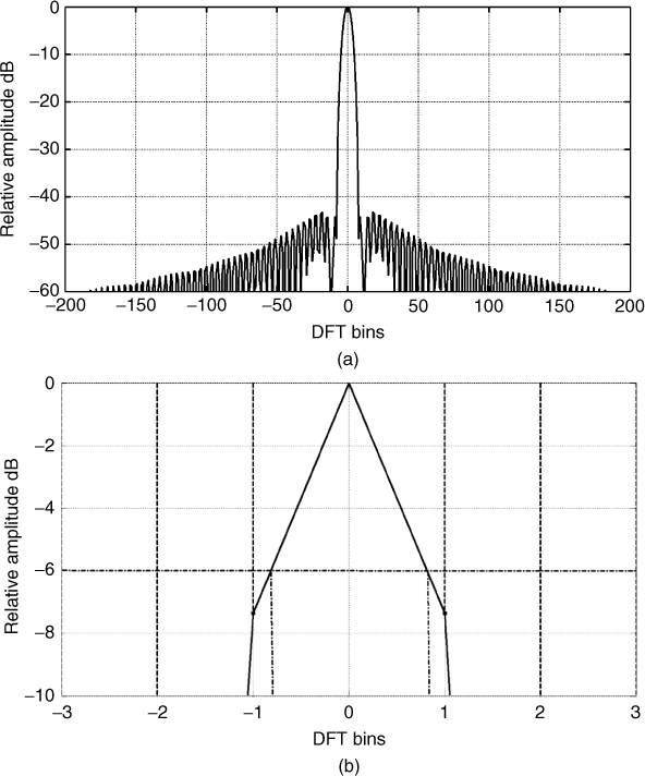
Table 5.1 gives three of their main properties: the peak sidelobe level, the rate of decay of sidelobes and the 6 dB width of the main lobe measured in DFT cells (or bins), as illustrated in Figure 5.2 for the Hamming window. Table 5.1 shows the trade-off between the different parameters where the window with the highest rate of decay of sidelobes has the largest mainlobe width, which affects the resolution of nearby frequencies but would give less interference between faraway frequencies.

Figure 5.2 Properties of the Hamming window: (a) overall window response and (b) 6 dB width.

In implementing the DFT, the fast Fourier transform (FFT) algorithm is usually employed due to its speed. Most FFT algorithms require the number of points to be a power of 2. Thus, if the length of data is less than a power of 2 it is usual to pad the data with zeros to the next power of two. Zero padding does not generate new information. However, it does provide interpolation between the original data points, which can be helpful in obtaining a finer estimate of some of the channel parameters.

5.3 DFT Analysis of the FMCW Channel Sounder Using a Heterodyne Detector

In this section analysis of the digitized output of the FMCW sounder using the DFT is shown to give the impulse response, the frequency response, the delay Doppler function and the Doppler spread. Examples pertinent to ultra-high frequency (UHF) indoor and outdoor environments in the 2 GHz band and to the HF band for propagation via the ionosphere are given to highlight the particular requirements of different radio channels.

5.3.1 Snapshot Impulse Response Analysis

In Chapter 3 it was shown that the output of the heterodyne detector in the presence of multipath propagation is the sum of CW signals whose frequencies (referred to as beat note) are related to the time delay difference between the reference sweep and the received sweep and whose amplitudes are proportional to the attenuation suffered over the radio path. To resolve the multipath components the signal is spectrum analyzed using the DFT where the frequency axis is rescaled into a time delay by multiplying with T/B, where T is the duration of the sweep (chirp) in seconds and B is the bandwidth of the sweep in hertz.

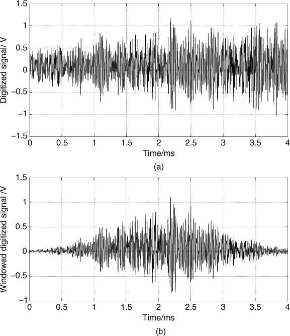
An example of a digitized time series data from a snapshot measurement at 2 GHz with 60 MHz bandwidth and 4 ms sweep time is displayed in Figure 5.3a, where the ADC converter output has been scaled by the number of bits and converted to voltage. Figure 5.3b displays the corresponding windowed data using the Hamming window. The effect of the window is seen to reduce the contribution of the signal on the edges, which results in a reduction of the amplitude of the resolved components as illustrated in Figure 5.3c for both the weighted and unweighted spectrum. Figure 5.3d displays the spectrum plotted versus the time delay where the zero time delay has been set to indicate the arrival time of the first multipath component.

Figure 5.3 Time series and corresponding spectrum: (a) unweighted after ADC, (b) weighted with Hamming window, (c) spectrum of weighted and unweighted signal and (d) spectrum of weighted signal with the frequency axis scaled to give the time delay.

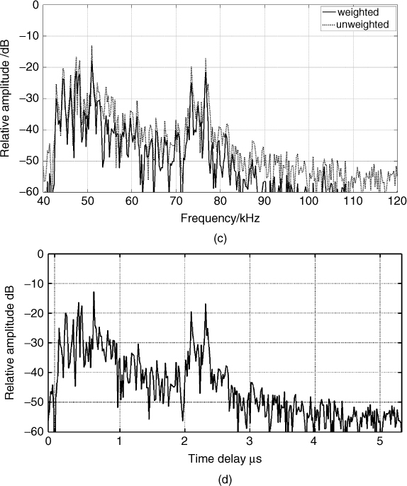
For UHF applications, the choice of the window function depends on the instantaneous dynamic range of the sounder. For example, for a dynamic range of 40 dB the best time delay resolution is obtained by the Hamming window.

5.3.1.1 Impulse Response versus Frequency

Since the time series signal at the output of the heterodyne detector is not compressed in time, it is possible to divide it into sections that correspond to frequency sections of the transmitted signal. This mapping can be achieved using the sweep rate. For example, in Figure 5.3a, the 4 ms time series data correspond to the 60 MHz swept bandwidth at 2 GHz. To estimate the impulse response of 5 MHz sections, the 4 ms time series data can be divided into 12 sections with 333.33 µs time duration and spectrum analyzed as shown in Figure 5.4a for all the 12 sections and Figure 5.4b for the first frequency section.

Figure 5.4 (a) Impulse response for 12 frequency sections obtained from a single time series of a single sweep and (b) impulse response for the first frequency section.

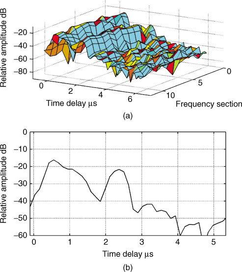
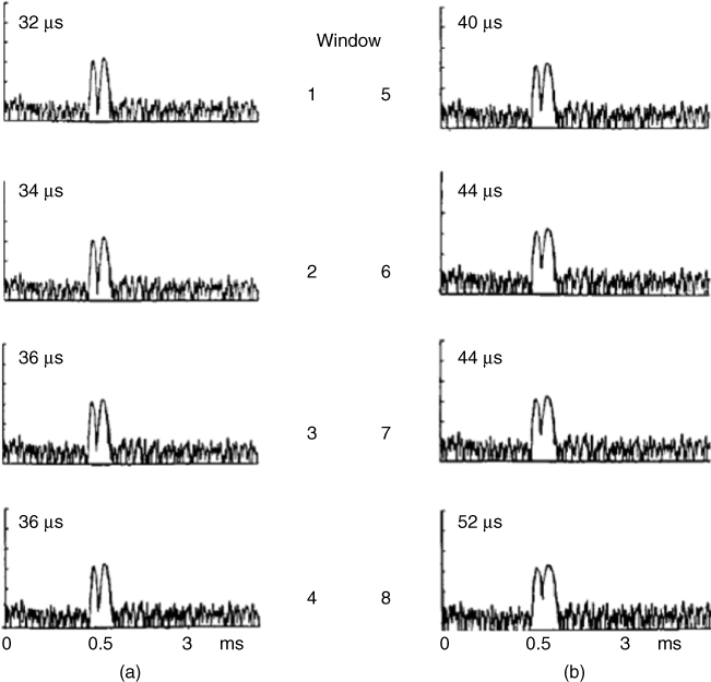
The division of the time series has two effects. The first is a reduction of the time bandwidth product by a factor equal to L² where L is the number of sections. This in turn reduces the processing gain by 10 log₁₀ L². The second effect is the reduction of the time delay resolution of the multipath components by L, as can be seen by comparing Figures 5.3d and 5.4b. This technique is widely used in ionospheric propagation to obtain ionograms from FMCW channel sounding data. In ionospheric propagation the choice of the window function has additional effects when estimating pulse dispersion of the two magneto-ionic waves, that is pulse broadening due to the phase nonlinearity of the channel. Figure 5.5 shows the variations in the broadening of the 6 dB width of the pulse for a 500 kHz signal centred at 7.63 MHz for windows 1–8 from Table 5.1. From the figure, it is seen that although the first window has the largest width it gave the smallest estimate for the 6 dB width of the pulse, whereas the Von Hann window gave the largest width. Due to the proximity of the two magneto-ionic waves, the rate of decay of sidelobes appears to have a more significant effect on the resolution of the two waves than the width of the main lobe of the window. It is therefore necessary to estimate the desired parameter from measurements using different window functions and subsequently choose the appropriate window. For UHF propagation in terrestrial environments, the effect of phase nonlinearity is negligible in comparison with the ionosphere. Parameters such as the RMS delay spread and the width of the overall PDP are of interest and the choice of the window function is related to these parameters rather than the width of a single component.

Figure 5.5 A 500 kHz signal processed with different window functions: (a) windows 1–4 and (b) windows 5–8 in Table 5.1 [3].

Source: Salous, S. and Khardra, L., (1989), Measuring the coherence of wideband dispersive channels. Journal of Electronics and Communications, Volume 1, Issue 5, pp 205–209. Reproduced with permission from IET.

5.3.2 Frequency Response Analysis

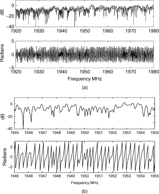
The DFT is also used in the estimation of the channel frequency response. The time series data are analyzed first with the DFT to obtain the impulse response. This is performed without the window function and without zero padding. Subsequently a second DFT is applied on half the number of points. If zero padding is applied, the additional points added at the end of the time series have to be subsequently removed. The result of the second DFT is the magnitude and phase of the frequency response, as illustrated in Figure 5.6 for the time series data of Figure 5.3a. Figure 5.6b is a zoomed-in section around the centre where the phase is seen to undergo a phase reversal when the magnitude goes through minima and maxima.

Figure 5.6 Magnitude and phase of the frequency response obtained via the double DFT (a) over the entire swept bandwidth of 60 MHz and (b) zoomed in section around 1950 MHz.

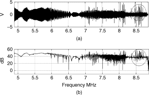
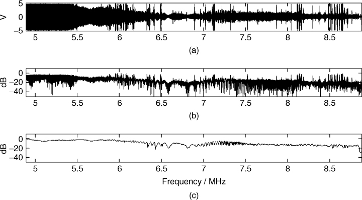
In ionospheric propagation, it is not always possible to apply the double DFT technique in particular if a wide bandwidth is covered since the HF spectrum is highly congested. This is illustrated in Figure 5.7, where the raw data prior to processing in panel (a) and the frequency response following the double DFT in panel (b) both show the frequency ranges that are affected by interference, such as in the encircled area around the 8.5 MHz band.

Figure 5.7 Raw HF time series data and corresponding envelope as detected from double DFT processing.

For this application it is necessary to employ a technique that alleviates the effect of interference on the estimated frequency response. This can be achieved by analyzing the data in a manner to that used for ionograms, that is via the DFT where each sweep is divided into L sections and the complex values of the identified multipath components are stored. The signal to noise ratio (SNR) in the spectrally analyzed sections can be enhanced by clipping the peaks of the interference [4]. The choice of the number of sections depends on the parameter to be estimated. For example, to evaluate the polarization bandwidth it is necessary to filter the required mode, say the 1F₂ mode, and then to choose a section length that does not resolve the ordinary and extraordinary waves. This usually implies a small bandwidth that does not enable the resolution of the two magneto-ionic components but is sufficiently large to give appropriate SNR to identify the resultant peaks. Since the time delay separation between the two magneto-ionic waves varies with frequency as they come closer together and then separate farther apart, this condition cannot be readily met. The other consideration in estimating the polarization bandwidth is to identify the separation between the minima. The larger the number of sections the more accurate is the estimation of the depth of the minima in the frequency function and their separation.

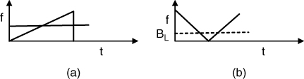
The division of the sweep into sections can be viewed as a filter of bandwidth B/L moving across the swept bandwidth B. Therefore, although it is desirable to divide the sweep into many sections to obtain fine frequency resolution, the compressed pulse peak power will decrease, resulting in the signal being masked in ranges with high interference. The interference of CW signals to FMCW sounders has been studied in detail in [5]. Figure 5.8 illustrates the processing of an interfering CW signal in the heterodyne detector, which generates a variable frequency as sketched in Figure 5.8b. By passing the signal through a filter with bandwidth equal to B_L only a portion of the power passes through the filter, as given by:

5.5

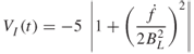
where V_I is the interference voltage, is the sweep rate and B_L is the filter bandwidth of the spectrum analysis. Thus, for a constant sweep rate, the interference suppression can be increased by decreasing B_L or equivalently decreasing the number of sections, since:

5.6

Figure 5.8 (a) CW interfering signal at input of the heterodyne detector and (b) output of the heterodyne detector due to the CW signal.

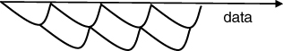
The conflicting requirements of a large section size to reduce interference and a small section size to measure more accurately the frequency response of the channel can be reconciled by overlapping the analyzed sections as illustrated in Figure 5.9 [6].

Figure 5.9 Overlap processing of time series data.

By moving the filter of bandwidth B/L along the frequency axis with increments either equal to half (50 % overlap) or quarter (75 % overlap) its bandwidth, the following is achieved: (i) the number of samples is increased by a factor of two or four for 50 % and 75 % overlap respectively; (ii) the degree of interference suppression, which is governed by the corresponding basic section length, is increased and (iii) an event occurring on the edge of the section and unseen owing to the weighting window would be resolved in the next overlapping section. Figure 5.10 shows the processing of a 4 MHz signal with interference from other users of the channel at several frequency bands. Panel (a) is the raw data, panel (b) the amplitude of the frequency response obtained via the double DFT and panel (c) the amplitude of the frequency response obtained from a single DFT with 75 % overlap of frequency sections with 3.9 kHz length.

Figure 5.10 (a) Digitized time series, (b) fading envelope from double DFT and (c) fading envelope from detecting the peaks after a single DFT with overlap processing.

5.3.3 Estimation of the Delay Doppler Function

Doppler shift occurs due to the change of path length as a function of time from the movement of the transmitter and/or receiver or the reflector. Thus Doppler estimation requires several snapshots over an adequate interval of time obtained at time intervals separated by T, where T is chosen to satisfy the sampling theorem such that 1/T ≥ twice the maximum expected Doppler shift. For example, a snapshot repetition rate of 250 Hz covers ± 125 Hz maximum Doppler shift.

For the FMCW heterodyne detector output, the delay Doppler function is obtained via a double DFT where the first DFT is performed on a snapshot basis to obtain the complex impulse response at time t_i where the real part is equal to and the imaginary part is equal to . By processing consecutive snapshots the time-variant impulse response can be obtained as in the following equation and illustrated in Figure 5.11a for measurements in the UHF band for 250 impulse responses obtained over 4 ms each giving a 1 second observation time:

5.7

After discarding half the number of delay bins due to symmetry, a DFT is applied to each time delay bin of the complex impulse response to estimate the Doppler shift. This gives the delay Doppler function where each time-delayed component is associated with its own Doppler shift, as shown in Figure 5.11b. To reduce the level of the sidelobes, windows are applied prior to the DFT operation. The delay Doppler function can then be used to obtain the Doppler spectrum where the magnitude squared values are summed over the time delay variable as in Figure 5.11c. Similarly summing the delay Doppler function over the frequency shift variable gives the average PDP as in Figure 5.11d. Alternatively, the PDP can be obtained directly from the time average of the magnitude squared of N impulse responses as:

5.8

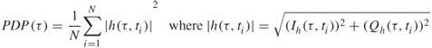
Figure 5.11 (a) Time-variant impulse response, (b) delay Doppler function, (c) Doppler spectrum and (d) average power delay profile.

In estimating these functions, the observation time has to be chosen appropriately, as will be discussed in Section 5.8. Generally speaking, the longer the observation time, the higher is the resolution in the Doppler shift domain as frequency resolution is inversely proportional to the time interval of the spectrally analyzed data. It is, however, important to ensure that the time interval used in the analysis is chosen such that the Doppler frequency does not move the multipath component to a different time delay resolution bin. This effect will be discussed further in Section 5.8.2. Phase noise in the receiver's local oscillators would appear as a frequency shift and would broaden the main peak. Hence, the integration time or the number of snapshots N to be used in the Doppler analysis should be chosen taking into account the speed of the reflector, the phase noise of the oscillators and the time drift of the frequency standards used in the measurement system.

5.4 Spectral Analysis of Network Analyzer Data via the IDFT

In general a two-port vector network analyzer gives the complex frequency response of the channel when two separate antennas are connected one to each port. The complex frequency samples can be either converted to magnitude and phase to obtain the frequency selectivity of the channel or can be analyzed via the inverse DFT to obtain the impulse response. Figure 5.12 shows an example of a measurement over an 800 MHz bandwidth in an indoor environment analyzed to give the impulse response. As in the case of the heterodyne detector the complex frequency function is multiplied by a window function prior to spectral analysis to reduce the level of the sidelobes of the sin x/x function.

Figure 5.12 (a) Magnitude of the complex frequency response and (b) impulse response obtained via the IDFT.

5.5 DFT Analysis of CW Measurements for Estimation of the Doppler Spectrum

For a single reflector, if the received signal is quadrature demodulated then the in-phase and quadrature components for a Doppler-shifted CW signal are given by:

5.9

These can be used to obtain the phase function as in:

5.10

The Doppler frequency is then evaluated from the derivative of Equation (5.10) with time, which can be obtained from the difference between consecutive phase samples. However, if a number of components are present, as in the case of multiple reflectors, it would not be possible to separate them and spectrum analysis of the received signal as in Equation (5.9) over the CIT would be required to obtain the Doppler spectrum. Similar to the case of multipath resolution, the data are weighted with a window function prior to the DFT processing.

5.6 Estimation of the Channel Frequency Response via the Hilbert Transform

Analysis thus far of the output of the FMCW heterodyne detector used the DFT to obtain the various channel functions. An alternative is to apply the Hilbert transform to the received signal on a snapshot basis to obtain the complex envelope, which can then be used to estimate the magnitude and the phase of the frequency response. This can be seen by considering a narrowband bandpass signal centred at as in:

5.11

If the bandwidth of A(t) is sufficiently narrowband such that , to detect A(t) we generate the analytic signal as:

5.12

by adding the Hilbert transform of Equation (5.11) and taking the magnitude as in:

5.13

The Hilbert transform shifts each frequency component in the signal by 90°.

Therefore, by taking the Hilbert transform of the time series at the output of the heterodyne detector of an FMCW sounder, it is possible to estimate the envelope of the frequency response. This is applicable when the beat notes at the output of the detector start at a sufficiently HF with respect to the envelope that the narrowband assumption holds. For short range applications this can be achieved by offsetting the start of the reference sweep.

5.7 Parametric Modelling

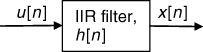
The DFT processing assumes that the signal outside the observation interval is zero, which is equivalent to multiplication by a rectangular window. To avoid this truncation effect, modern spectral analysis techniques such as MA, AR and ARMA, generally known as parametric models, extend the signal outside the observation interval through modelling the signal as the output of a causal linear filter. The general form of parametric models is to assume that the time series data x[n] represent the output of an infinite impulse response (IIR) filter, h[n] due to a white noise process u[n] of zero mean and variance as in Figure 5.13. The input and output relationship of this filter is in the form of a recursive linear difference equation with complex coefficients as in:

5.14

Figure 5.13 IIR filter representation of parametric models.

Following from the theory of linear filters, the output can also be represented by the convolution sum as:

5.15

Taking the z-transform of Equation (5.14) gives:

5.16

The system transfer function is then given by:

5.17

where z₁, z₂,…, z_M are the zeros and z_1p, z_2p,…, z_pP are the poles of the transfer function that give rise to minima and maxima respectively.

The frequency response H(f) can then be evaluated from:

5.18

where T is the sampling interval. This gives the frequency response of the filter, as in:

5.19

Since the power spectral density of white noise is a constant, the power spectral density of the signal , after scaling by T, can be related to the filter's frequency response as in:

5.20

Thus specification of the parameters a[k] and b[k] and the variance of noise is equivalent to specifying the spectrum of the signal x[n] [7].

Equations (5.14) and (5.16) describe the general ARMA model where a[k] and b[k] form the AR and the MA portions of the model respectively. If all the AR parameters are zero the resulting model is an MA model and the transfer function of the filter has zeros only, which results in a spectral estimate with broad peaks and sharp nulls. The MA power spectral density does not model narrowband spectra well and is not, therefore, a ‘high resolution’ spectral estimator. When the MA parameters are zero the resulting model is AR and the filter's transfer function has poles only. This gives sharp peaks in the response of the model, which are usually associated with high resolution. The ARMA model results in both sharp peaks and sharp nulls and is usually recommended when the SNR is low since it requires fewer parameters to model the data [7], [8].

Taking the inverse z-transform of Equation (5.17) gives the linear difference equation of the filter in the time domain as:

5.21

where K is the number of data samples used in the model.

5.7.1 ARMA Modelling

An algorithm for ARMA modelling is the Prony algorithm, which forms a set of linear equations. Considering Equation (5.21), the algorithm first solves for the equations from M + 1 up to K − 1. Since M is the number of a[k] coefficients, this enables the substitution by zeros in these equations, which can then be solved using the least squares error to find the b[p] coefficients. These are then placed in the first M + 1 equations, which are then solved for a[k]. The unit sample response of the filter then gives an estimate of the data, . Subsequently, the frequency response of the filter can be obtained by calculating H(z) at equally spaced points around the unit circle or through the DFT of the estimated sequence. For good estimation the model orders are between K/3 and K/2 for P and between K/10 and K/3 for M. For lower values of M the signal level decreases and for very low values spurious peaks may appear, whereas very high values of M raise the noise floor.

5.7.2 AR Modelling

Since the coefficients a[k] in Equation (5.21) are zero, the estimation of the parameters for the AR model result in a set of linear equations, which has a computational advantage over ARMA and MA parameter estimates. A number of algorithms are available for the estimation of the parameters of the AR model, which include the forward backward least squares algorithm (FB), the Burg method (modified covariance), the covariance method and the Yule Walker method. A detailed review of the various techniques and their properties can be found in [8]. Briefly stated, the Yule Walker algorithm has the least resolution whereas the FB method offers the best resolution for sinusoids. The covariance method gives false peaks and greater perturbations of spectral peaks from their correct frequencies than other AR estimation approaches. The Burg algorithm exhibits spectral line splitting and introduces biases in the frequency estimates. In contrast, the FB method has less bias in the frequency estimates of spectral components, reduced variance in frequency estimation and absence of spectral line splitting [8]. Similar to the ARMA model, the recommended model order is between K/3 and K/2.

5.7.3 Practical Implementation of Parametric Modelling

Since the recommended order model is generally high (K/3–K/2) this can be computationally inefficient for a large number of data samples. To reduce the computation time, data reduction, for example via prefiltering, mixing down and decimation, can be applied to the data prior to modelling. The model order can also be chosen according to a predetermined error criterion such as the Akaike information criterion (AIC) and the minimum description length criterion (MDL) [7].

Another aspect to consider is that resolution and detection with the parametric techniques depend on the SNR, where modern spectral estimates are often no better than those obtained with the DFT for low SNR values [7]. Noise broadens the spectral peaks and displaces them from their true positions.

5.7.4 Parametric Modelling for Interference Reduction

In Section 5.3.2 the effect of interference on the estimation of the frequency response of the channel was discussed. In this section we study the effect of interference on the estimation of the impulse response and the PDP and introduce parametric modelling for reducing its effects on the output of FMCW heterodyne detectors. From Equation (5.5), an interfering CW signal generates a voltage that is related to the bandwidth of the filter in the detector as the interfering signal sweeps across the filter. Thus in the first instance interference reduction can be achieved by narrowband filtering the wanted signal. For example, having identified the frequency ranges over which the signal or multipath components are present, these can be filtered prior to further processing. Another simple alternative is to use interference free sweeps to extract the channel response.

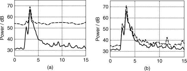
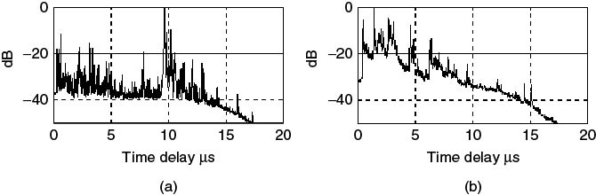
Following filtering, the data can be processed with the DFT to obtain the impulse response, which when averaged over a number of sweeps gives the PDP as in Equation (5.8). Figure 5.14a illustrates the effect of interference on the PDP for two 5 MHz frequency sections with and without interference obtained from a 60 MHz sweep in the UHF band. The effect is seen to raise the noise floor by about 25 dB, thus reducing the dynamic range of the measurement and reducing the range for which the channel parameters can be computed. As stated in Section 5.3.2, the effect of interference can be reduced by clipping, as seen in Figure 5.14b, where now the difference in the noise floor between the interference free section and the clipped section is between 2 and 3 dB [9].

Figure 5.14 Effect of interference on the estimated PDP on two frequency sections: dashed line for section with interference and solid line for interference free section. PDP (a) without interference clipping and (b) with interference clipping [9].

Source: Salous, S., and H. Gokalp, (2007), Medium and large scale characterisation of UMTS allocated frequency division duplex channels, IEEE Transaction on Vehicular Technology, 56(5), pp 2831–2843. Reproduced with permission IEEE.

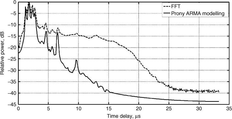
Alternative to clipping the peaks of the interference is to apply ARMA parametric modelling using the Prony algorithm following prefiltering of the required signal [10]. Figure 5.15 illustrates the raw data with in-band interference for a 2.1 MHz frequency section centred at 1975.5 MHz and the corresponding data generated from Prony modelling with 50 zeros and 100 poles. The data are now seen to be interference-free and this is confirmed from the PDP in Figure 5.16, which is obtained from FFT processing and from Prony ARMA modelling and gives a reduction of ∼15 dB in the noise floor. The figure also displays the PDP obtained by selecting the interference-free sweeps from the data. While this simple technique gives good results, it relies on interference time hopping, which cannot always be guaranteed. A second example with Prony ARMA modelling is shown in Figure 5.17 where the PDP has several multipath components and the modelled data are seen to match the multipath delays accurately, as obtained from the classical FFT processing except for a 1–2 dB amplitude difference for the strongest four components.

Figure 5.15 Raw data with interference (solid line) and Prony ARMA modelled data (dashed line) [10].

Source: Gokalp, H. and G. Y. Taflan, and S., Salous, (2009), In-band interference reduction in FMCW channel data using Prony modelling, Electronics Letters., 45 (2), pp. 132–133. Reproduced with permission of IET.

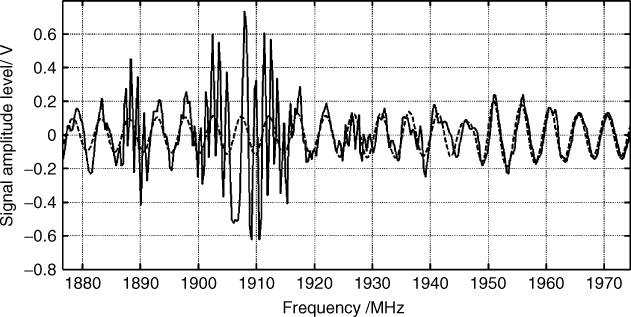
Figure 5.16 PDP obtained from FFT processing with all sweeps and with interference free sweeps only (clean sweeps) and from Prony ARMA modelling [10].

Source: Gokalp, H. and G. Y. Taflan, and S., Salous, (2009), In-band interference reduction in FMCW channel data using Prony modelling, Electronics Letters., 45 (2), pp. 132–133. Reproduced with permission of IET.

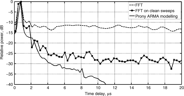
Figure 5.17 PDP obtained from data with interference processed with the FFT and with Prony ARMA modelling [10].

Source: Gokalp, H. and G. Y. Taflan, and S., Salous, (2009), In-band interference reduction in FMCW channel data using Prony modelling, Electronics Letters., 45 (2), pp. 132–133. Reproduced with permission of IET.

5.7.5 Parametric Modelling for Enhancement of Multipath Resolution

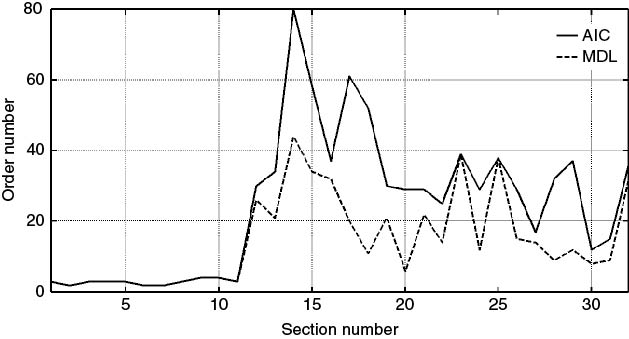
One of the other applications of parametric modelling is to enhance the resolution of multipath components. AR modelling is generally considered a high resolution approach as it enhances the peaks of the spectrum due to the poles in the transfer function. To illustrate the enhancement in resolution, 4 MHz sweep data centred at 6.88 MHz obtained over a UK HF link are processed with both the FFT and AR modelling [4]. Prior to processing the raw data are filtered to include the 1F2 mode using two filters to follow the variations of the group time delay with frequency, as shown in Figure 5.18. To enhance the detection of the AR model, the interference in the data is clipped prior to processing, as illustrated in Figure 5.19a and b, which displays the data prior to and after clipping. The presence of interference in the data is evident in particular in the second half of the sweep. To reduce the number of samples the data are down-converted, filtered and decimated. Subsequently, each 4 MHz sweep is divided into 32 sections to obtain ionograms with a theoretical 8 µs time delay resolution. Both FFT processing and AR modelling are applied to each section according to the selected model order based on both the AIC and the MDL criteria and the results are as shown in Figure 5.19c and d for the FFT and the AR modelling respectively. The corresponding AR model order is given in Figure 5.20 for both criteria, which are considerably much lower than the recommended number of K/2–K/3, which would have been equal to 170–256. In addition, the MDL criterion is seen to give a lower order number than the AIC. From Figure 5.19c and d, the more defined peaks in the ionogram as obtained from the AR model are evident and clearly provide an enhancement in the resolution between the two magneto-ionic waves.

Figure 5.18 Filters used to select the 1F2 mode from the raw data [4].

Source: Salous, S., (1997), On the potential applicability of auto-regressive spectral estimation to HF chirp sounders, Journal of Atmospheric and Solar-Terrestrial Physics, Vol. 59, No. 15, pp 1961–1972. Reproduced with permission of Elsevier.

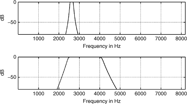
Figure 5.19 (a) Data after filtering, (b) filtered data clipped for interference reduction, (c) ionogram with FFT processing and (d) ionogram with AR modelling.

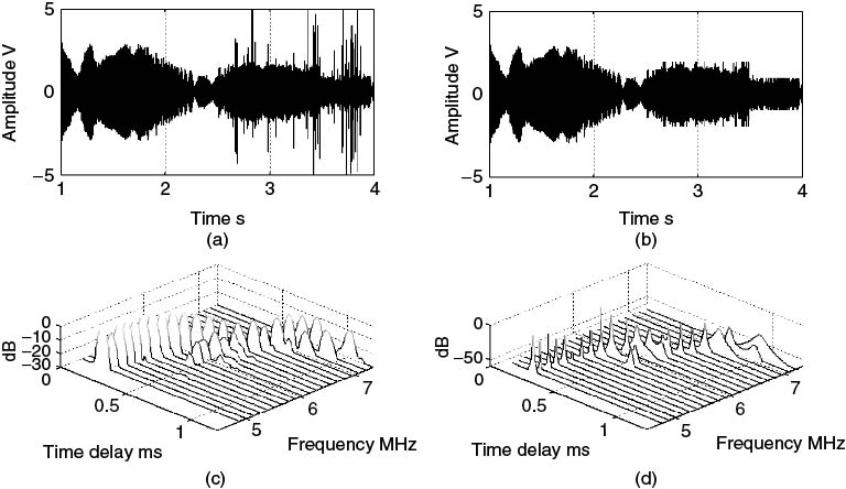
Figure 5.20 Model order selection according to the AIC and MDL criteria for the ionogram in Figure 5.19.

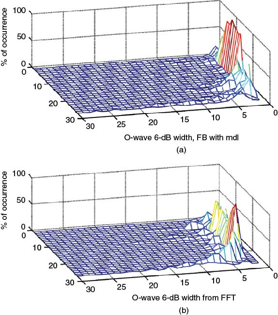
A measure of the enhancement in resolution is the 6 dB width of the pulse identifying the multipath component following spectral analysis. Figure 5.21 shows the distribution of the 6 dB width of the ordinary wave as measured both from the DFT with the Von Hann window and with the AR FB method using the MDL criterion across 27 frequency sections for the same set of 4 MHz data. The narrower width using the AR method is evident from the figure, which indicates a higher resolution. This enhancement is obtained at the expense of additional computations in comparison to the DFT.

Figure 5.21 Distribution of measured 6 dB width of the ordinary wave in bins where each bin is equivalent to 2 µs: (a) AR modelling and (b) FFT processing [4].

Source: Salous, S., (1997), On the potential applicability of auto-regressive spectral estimation to HF chirp sounders, Journal of Atmospheric and Solar-Terrestrial Physics, Vol. 59, No. 15, pp 1961–1972. Reproduced with permission of Elsevier.

5.8 Estimation of Power Delay Profile

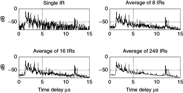
In radio channel studies, the impulse response of the channel at any instant in time is assumed to be derived from a stochastic process, which over short periods of time is considered to be wide-sense stationary (WSS). Therefore, time averaging or spatial averaging is employed to obtain the PDP from a number of channel impulse responses N, as given in Equation (5.8). This has the effect of reducing the noise peaks, which are assumed to be uncorrelated between measurements and uncorrelated with the wanted signal. The effect of averaging is illustrated in Figure 5.22, which displays an instantaneous PDP obtained from a single impulse response and PDPs obtained from averages over 8, 16 and 249 instantaneous PDPs. The degree of noise smoothing is related to N where, for Gaussian additive noise with zero mean and standard deviation (see Appendix 1 for the Gaussian distribution), the averaged noise standard deviation is reduced to , which is equivalent to 20 logN enhancement in SNR. The choice of N is a compromise between noise reduction and signal detection where N is chosen such that the signal component remains coherent over the averaging interval. It is therefore generally accepted that for the estimation of the PDP an average over time or space is performed. An appropriate threshold level is subsequently set for the detection of the multipath components, which are included in the estimation of channel parameters such as the RMS delay spread and average delay.

Figure 5.22 Power delay profile obtained from a single impulse response IR or from an average over 8, 16 and 249 instantaneous PDPs obtained from consecutive IRs.

However, it is important to note that while averaging offers the advantage of noise reduction, it is not always feasible to average consecutive PDP is, for example, in ionospheric propagation, where ionograms are obtained without averaging and the noise effects are reduced by narrowband filtering of the different modes as shown in Figure 5.18 in Section 5.7.5. Another consideration arises when an insufficient number of impulse responses are acquired, which does not enable appropriate time or spatial averaging and the channel parameters have to be estimated from a single snapshot PDP.

Thus it is necessary to determine two parameters:

5.8.1 Noise Threshold

Equation (5.8) states that the PDP represents the magnitude squared of the complex impulse response or an average thereof. Neglecting the effect of interference and considering thermal noise in the complex impulse response, it can be assumed that the noise components of the in-phase and quadrature components are independent Gaussian distributed with zero mean and variance, giving a Rayleigh distributed envelope with a PDF as illustrated in Figure 5.23 and expressed by:

5.22

Figure 5.23 Rayleigh distribution for σ = 1.

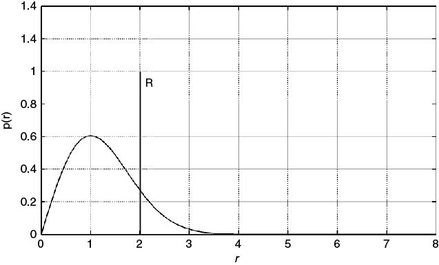
To establish a noise threshold level R for the detection of the multipath components, a certain probability of error is allowed where an error occurs if the threshold is too low and a noise peak is detected as a signal or if the threshold is too high and the signal is missed. Using radar terminology these situations are referred to as false alarm or a miss respectively. For a Rayleigh distribution the median and the mean are given by and respectively. For a threshold level equal to R, as illustrated in Figure 5.23, a false alarm occurs if the magnitude of noise exceeds R. Thus the probability of a false alarm per sample P_f is given by:

5.23

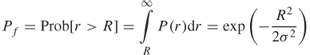
The value of the threshold R is chosen to meet a certain acceptable error rate. For example, an error in 100 single snapshot PDPs with 2000 samples per PDP sets the P_f to 5 × 10⁻⁶ (number of errors/total number of samples). Using Equation (5.23) and evaluating the noise variance from the measurements enables the estimation of R. One possibility is to set the threshold level , where R is a constant as employed in radar [11]. In this case, the threshold level is raised and lowered from one impulse response to another to maintain a constant false alarm rate (CFAR), given by:

5.24

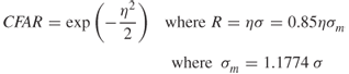
For example, to detect an error in 250 single snapshot PDPs with 1000 data points per PDP gives P_f = 4 × 10⁻⁶. Using Equations (5.23) and (5.24) gives a value of η = 4.98 or 13.95 dB. From the measurements, the median value of the samples for each impulse response are computed and then multiplied by to obtain the threshold level. Figure 5.24 gives the noise threshold level as computed from Equation (5.24) for each single snapshot PDPs, which shows a wide range of variations of the threshold level between PDPs.

Figure 5.24 Variations in the threshold level for 250 consecutive PDPs each obtained from a single snapshot or impulse response.

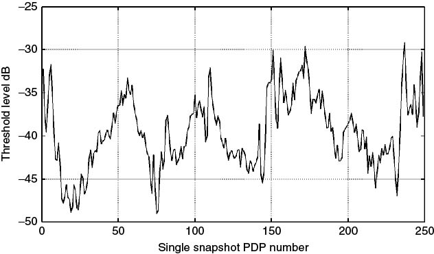
The difference between the threshold level for the PDP obtained from a single impulse response and that obtained from the average of 250 single PDPs is shown in Figure 5.25. For the average delay profile, the lower threshold level corresponds to the median value whereas the higher level is found from the CFAR equation (Equation (5.24)). Similarly, for the PDP obtained from the single impulse response the threshold is found from Equation (5.24).

Figure 5.25 Power delay profile obtained from an average of 250 single PDPs (a) and from a single impulse response (b).

Figure 5.25 indicates that applying the criterion of the CFAR threshold is appropriate for both cases although it is unnecessarily high for the averaged profile as the noise peaks have been considerably reduced by smoothing. If the threshold level is set too high, then signals can be missed and it is necessary to estimate the probability of a miss as given by:

5.25

where Q is the Marcum's Q-function [12, p. 585], and SNR_k are the power and SNR in the kth bin respectively and the Marcum function is given by:

5.26

In the event that the threshold level set by the CFAR significantly reduces the dynamic range of the PDP or an insufficient number of impulse responses are collected to enable time averaging to reduce the effect of noise, other criteria need to be applied. In [11], it is postulated that if the range bin contained a signal then the likelihood is that the adjacent bins also had a signal component and the variations in the signal level in these bins are correlated. Whereas if the range bin contained a noise impulse it is unlikely to be correlated to the adjacent rang bins. Thus the criterion for detecting an echo is set such that if the threshold is exceeded in three consecutive single PDPs, and that at least one of the neighbouring points also exceeded the threshold level in all three PDPs, then the range bin has a signal and a PDP is generated from the average of all three single PDPs. Using this algorithm, the probability of false alarm is now given by:

5.27

Thus for an error of 4 × 10⁻⁶, the threshold should be set at , which is 6.4 dB above the threshold or ∼5 dB above , which is a lower level than set by Equation (5.24).

5.8.2 Stationarity Test

One of the important considerations in estimating the PDP is the spatial distance or time span to average over, or equivalently the number of impulse responses N used in the averaging in Equation (5.8). PDPs obtained from both types of averaging exhibit different properties where the temporally averaged profiles tend to have finer and denser multipath components and the spatially averaged profiles are smoother, as illustrated in Figure 5.26 [13].

Figure 5.26 Power delay profile obtained from (a) time average and (b) spatial average [13].

Source: Salous, S., Gokalp, H., Dual frequency division duplex sounder for UMTS frequency division duplex channels. IEE Proc. Commun. Vol. 149, No. 2, April 2002, pp117–122. Reproduced with permission of IET.

In spatial averaging for the estimation of the PDP, it is usual to average over tens of wavelengths of travel distances where the WSS assumption holds. Different figures are reported in the literature for averaging distances varying from 3 to 100s of wavelengths [9, 14–17]. Others reported time averages with the transmitter and receiver stationary and others reported time averages with movement [18–20].

Figure 5.27 illustrates the variations of the PDP obtained along a main street perpendicular to the line of sight (LOS) in the city of Durham, UK, over 30 m in 15 seconds with a 60 MHz bandwidth and a PDP every 4 ms. Two effects can be seen: the first is that the time of arrival of the first component moved with distance and the second effect is the variations of the multipath structure where some components appeared and then disappeared with differences between the two frequency bands.

Figure 5.27 Instantaneous power delay profiles over 30 m of travel.

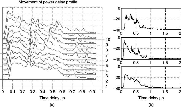
Dividing the data to obtain 10 average PDPs, the movement and the variations of the multipath structure can be seen from Figure 5.28. While the first arriving component appears to have a steady decrease in the time of arrival, other components appear to be moving farther away. Figure 5.28b shows the difference between an average obtained over the first two metres of travel and the last two metres of travel and the overall average over the travelled distance, which illustrates the smoothing effect of averaging.

Figure 5.28 (a) Consecutive power delay profiles from 2 m spatial average and (b) PDP from the first 2 m (top), last 2 m (middle) and an overall average (bottom).

From Figures 5.27 and 5.28 it is clear that it is necessary to quantify the interval over which the data can be averaged. Two methods to determine the averaging time (distance) are:

5.8.2.1 RUN Test for WSS Processes

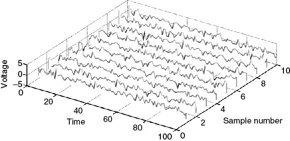
The study of the properties of stochastic processes requires having an ensemble of measurements obtained simultaneously as a function of time. For example, a set of measurements can be obtained by monitoring and recording the temperature every 5 seconds at 10 locations. The set of measurements represents the ensemble of the temperature variations and the data acquired at each location is referred to as a sample function. An ensemble of measurements of noise from 10 different noise sources is shown in Figure 5.29. Taking values at different instants in time t from all the sample functions in the ensemble generates the PDF of the random variable x, which can be used to estimate its moments, such as the mean and variance given by:

where p(x) is the PDF of x at one instant in time and the variance is found from:

5.28

The WSS assumption for small-scale characterization implies that the mean μ is a constant and that the autocorrelation function is only a function of the time shift. That is taking the average of the ensemble at t = t₁ and at t = t₂ gives the same value as expressed in:

where E represents the expected value of the ensemble:

5.29

The autocorrelation function gives a measure of the degree to which two samples of the same random process are related and its Fourier transform is the power spectral density of the process as in:

5.30

Other properties of a WSS process is that if the input of the linear time invariant (LTI) system is WSS then the output is also WSS and the input and output are related by:

5.31

In propagation studies when we estimate the radio channel response, an ensemble of simultaneous realizations is not available but rather samples of the channel response obtained consecutively in time. Therefore, statistical averages cannot be estimated, but rather time series averages as in:

5.32

Under the assumption that the process is ergodic, time averages are generally used to represent the process rather than statistical averages. In this case the time average is equal to the statistical average as in:

5.33

and the variance of the time average is zero since it is constant. Time series can then be analyzed to estimate averages, variances, autocorrelation functions and MAs.

Figure 5.29 Ensemble of sample functions representing 10 noise sources.

To test for WSS a statistical test called the RUN test can be applied to the time series data. To perform the test, the time series data are divided into N_i equal intervals where the data in each interval is considered independent. The mean and variance in each interval is then evaluated separately. The variance values are tested for an underlying trend by taking their median value and finding the values that fall above and below the median where the value is designated by a + sign or a − sign if it falls above or below the median value respectively (numbers equal to the median are removed). For example, if the variance values when tested against the median give the following sequence +++------+++ then the number of RUNs N_runs is equal to three:

5.34

with two positive RUNs N₊ and one negative RUN N₋. Subsequently, half the number of RUNs is entered into the table in [21, p. 396] to identify the acceptable low and high number of RUNs for low and high confidence levels, c_low and c_high respectively. If the number of computed RUNs N_runs falls outside these limits, as given in the following equation, then the hypothesis that the process is WSS is rejected; that is:

5.35

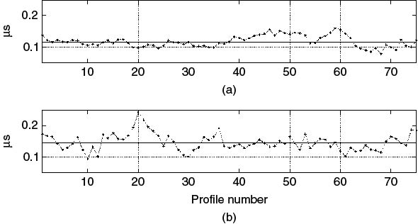
To apply the RUN test to radio channel time series data of consecutive impulse responses, we first estimate N_i average PDPs by dividing the data set into equal groups containing the same number of impulse responses. Subsequently, each PDP is used to compute the RMS delay spread, which is a measure of the second order central moment. The median of the computed RMS delay spreads is then evaluated and the number of RUNs is found. For the 30 m data in Figure 5.27, taking an average over 0.4 m gives N_i = 75 PDPs, which when used to estimate the RMS delay spread for a 30 dB threshold gives the results in Figure 5.30, where we find 15 RUNs with N₊ = 8 and N₋ = 7 for the downlink and 24 RUNs for the uplink with N₋ = 11 and N₊ = 13. For confidence levels of 0.05 and 0.95, with N_i = 75, we enter the table with the value of 37.5. Since this is not included in the table, we can take the average for the entries of 35 and 40 which give acceptable RUN values between 28 and 43. Since the number of RUNs for both the uplink and downlink are outside these limits, the data are considered nonstationary over the 30 m interval. To identify the stationary distance, different numbers of sections should be considered until the RUN test gives the stationary interval.

Figure 5.30 RMS delay spread variations about the median for (a) uplink and (b) downlink.

An alternative to testing the RMS delay spread from the PDP is to analyze the frequency response of the channel at a particular frequency. By taking complex samples at a single frequency to generate the time series, the stationarity of the process can be verified using the RUN test by dividing the time series into N_i sections and estimating the variance for each section from the real part of the samples [22].

5.8.2.2 Relationship between Maximum Doppler Shift and Time Delay Resolution of Sounder

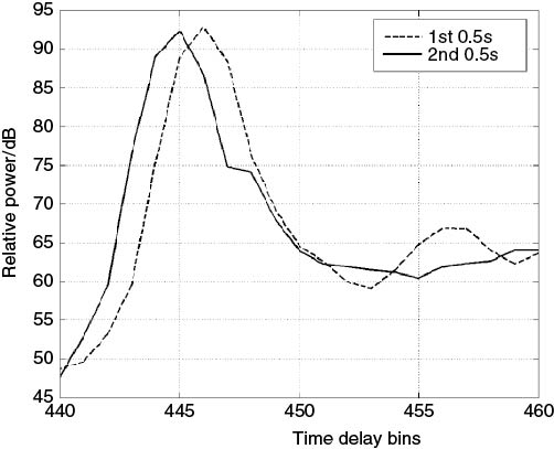
In this test, the distance travelled by the mobile in relation to the time delay resolution of the sounder is examined to estimate the averaging distance or time for obtaining the PDP. Similar to the definition of coherent integration time in radar applications the number of channel impulse responses that can be used in the average correspond to the duration (or distance) during which the multipath components do not move by more than half a delay resolution bin, which is then related to the maximum observed Doppler shift [9]. For example, for a 60 MHz bandwidth, the ideal range resolution is equal to 5 m. For 1 second of integration time, this limits the maximum Doppler shift to 33.3 Hz. For higher Doppler shifts, the time interval for averaging should be a fraction of a second, as shown in Figure 5.31 for a measurement with a 70 Hz Doppler shift where the movement of the peak from one time delay bin to another during the 1 second observation time is evident due to the high Doppler shift. This smears the delay profile where the same multipath component is detected in several range bins and affects the overall estimate of received power and RMS delay spread. Although this has not been explicitly stated in other reported measurements an average PDP over 5–30 m [14] and 5 m [15] were considered suitable when the corresponding resolutions of the sounders were 30 m.

Figure 5.31 Power delay profiles obtained from averaging over 0.5 second from a 1 second data set [9].

Source: Salous, S., and H. Gokalp, (2007), Medium and large scale characterisation of UMTS allocated frequency division duplex channels, IEEE Transaction on Vehicular Technology, 56(5), pp 2831–2843. Reproduced with permission IEEE.

5.8.2.3 Comment on the RUN Test versus the Coherent Integration Time Test

In [9] an average over 10 sweeps (40 ms) from vehicular data obtained in the city centre of Manchester were analyzed for both 60 MHz and 5 MHz resolutions. For 1 second of data this gives 25 PDPs, which corresponds to different spatial averages depending on the vehicle's speed. The number of RUNs was subsequently entered into the tables in [21] to determine the stationary distance for averaging. For 30–80 Hz Doppler shifts the spatial averaging distance as estimated from the RUN test should not exceed 3 m for the 60 MHz resolution, whereas for the 5 MHz resolution the stationary distance could be in excess of the distance travelled in the 1 second interval. This result is similar to the coherent integration time condition since the resolution obtained with the 60 MHz bandwidth is equal to 5 m resolution and thus the 3 m distance is within one resolution bin. For the 5 MHz bandwidth, the range resolution is equal to 60 m, which is far in excess of the distance travelled in 1 second.

5.9 Small-Scale Characterization

Small scale refers to the distance of travel or to the time interval over which the channel can be considered as WSS. As outlined in Section 5.8, this corresponds to a time series consisting of N impulse responses that can be used in the estimation of the PDP, the delay Doppler function and the average Doppler function. In Sections 3.2.2.1 and 3.2.2.3, the main parameters associated with the PDP were defined as well as the coherence functions. In this section we describe how to identify the start and end points of the PDP to be used in the computation for the average delay, RMS delay spread and delay window and illustrate the effect of the threshold on the estimated parameters. We then discuss the computation of the frequency coherence function.

Another important aspect is the representation of the time variations (time fading) of the multipath components within a single time delay resolution or at a particular frequency in terms of PDFs. Here we relate the choice of the suitable density function to the Kolmogorov–Smirnoff (KS) goodness of fit.

5.9.1 Time Domain Parameters

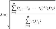
In Section 3.2.2.3 the definitions for the average time delay T_D and RMS delay spread, S were given in Equations (3.73) and (3.74) as:

where M is the number of samples per PDP and L is the index of the first arriving echo.

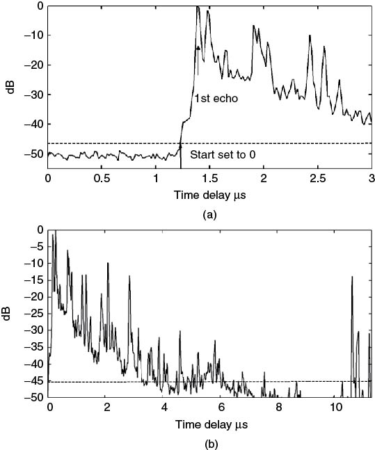
An important consideration in the estimation of these parameters is the noise threshold level, the dynamic range of the resulting delay profile, the time delay reference for the first arriving echo L and the number of time delay samples m to include in the PDP prior to L. Referring to Figure 5.32, following the estimation of the noise threshold, the ‘start’ and ‘end’ of the profile are identified. These refer to the first and last indices when the delay profile exceeds the threshold level. Figure 5.33a indicates the ‘start’ of the profile, which is set to 0 time delay by subtracting it from all the time delay indices, and τ_L, which refers to the time index of the first arriving multipath peak, which is now estimated with respect to the new time delay axis as seen in Figure 5.33b. Following the estimation of the start and end of the profile, only time delay bins that have components above the threshold level are used in the computation of PDP parameters.

Figure 5.32 Power delay profile with noise threshold indicating the start and end of the profile above the threshold.

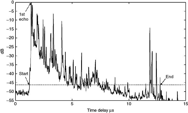
Figure 5.33 (a) Zoomed-in section on start of PDP in Figure 5.32 and (b) PDP of Figure 5.32 adjusted to zero time reference.

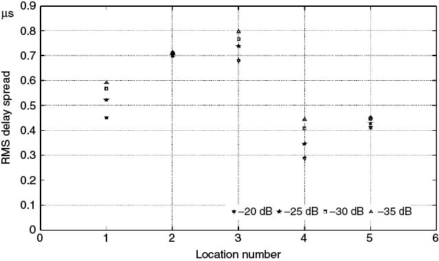
In Figure 5.32 the PDP has been normalized with respect to its own maximum. Although the figure displays the PDP in dB scale, the computations of the parameters are performed on a linear scale. Note that the normalization does not affect the results of the computation for the average delay or for the RMS delay spread as they are both divided by the overall power. Also, the correction due to the time delay of the first peak only affects the computation of the RMS delay spread. However, an important factor in the estimation of the time domain parameters is the dynamic range of the PDP and the setting of the threshold level with respect to the maximum. Figure 5.34 displays the effect of using different threshold levels which are between −20 dB and −35 dB down with respect to the maximum at five locations.

Figure 5.34 Effect of threshold level on the estimated RMS delay spread.

5.9.2 Estimation of the Coherent Bandwidth

In Section 3.5.2 the general coherence function was defined in terms of the expectation function , which could be simplified to obtain the time coherence function and the frequency coherence function under the assumptions of wide-sense stationary uncorrelated scattering (WSSUS), that is:

Under these assumptions the frequency correlation function is only a function of the frequency difference and can be related to the PDP by the Fourier transform as:

5.36

In the definition of the expectation functions in Chapter 3, the process is assumed to have zero mean.

An alternate definition of the coherence bandwidth can be estimated from the complex covariance of the channel frequency response at two frequencies separated by as given in the following equation where the process mean value is subtracted [23]:

5.37

Usually, the normalized autocovariance function is computed instead as in Equations (5.38) and used to evaluate the coherence bandwidth for different values below the peak:

5.38a

5.38b

where is the envelope of the received voltage at .

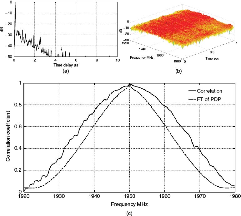
To illustrate the difference between the two methods we consider the PDP in Figure 5.35a, which has a main component with smaller components at a level below 20 dB from the main peak. Intuitively this should give a high correlation bandwidth as the effect of the smaller components on the resultant frequency response should be to produce small variations with frequency, as can be seen from Figure 5.35b. The difference between estimating the correlation function from Equations (5.36), (5.38a) and (5.38b) is shown in Figure 5.35c, where the Fourier transform (FT) of the PDP gives a smaller estimate of the coherence (correlation) bandwidth. Taking the 0.5 correlation value, the bandwidth from the covariance matrix is equal to 33.96 MHz versus 24.3 MHz from the FT of the PDP.

Figure 5.35 (a) Power delay profile, (b) time-variant frequency function and (c) frequency coherence function.

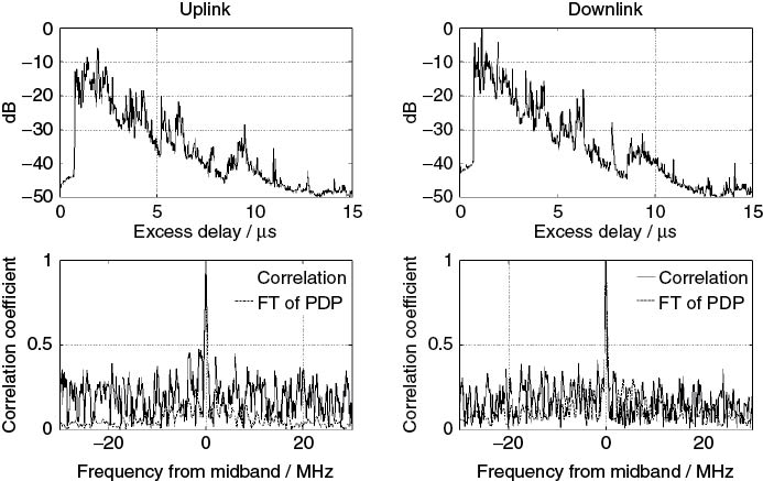
For other PDPs that exhibit a significant multipath structure as in the example shown in Figure 5.36 for the uplink (1920–1980 MHz) and downlink (2110–2170 MHz) of the universal mobile telecommunication system (UMTS) band, the main lobe of the correlation coefficient is seen to be similar with both estimation methods.

Figure 5.36 (a) Power delay profile for the uplink and downlink (b) and their corresponding correlation function.

5.9.3 Statistical Modelling of the Time Variations of the Channel Response

Thus far the channel function has been represented either in the time domain through its time-variant impulse response or through its time-variant frequency response. In either domain, the time variations can be represented by a statistical PDF such as Rayleigh, Weibull, Rician, log-normal, and so on, either by considering the envelope at a particular frequency or by taking the values at time delay bins, which represent a group of multipath components. When a single spectral line (frequency) is considered, the fading characteristics represent the contribution of all the multipath components. If, on the other hand, the time-variant impulse response is considered then each time delay bin consists of a subset of the unresolved multipath components in that particular delay interval. In this case, each delay bin above the noise threshold can be analyzed separately.

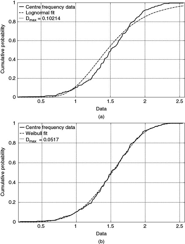
Regardless of which time-variant function is used, a time series is obtained from N channel functions either at a single frequency or a single time delay bin and then the best fit to the resulting random variable is found. In Figure 5.37 the envelope of the received signal at the centre frequency of transmission is displayed. The fit to the empirical data points using both the Weibull distribution and the log-normal distribution are given in Figure 5.38. To establish the goodness of fit, tests such as the KS test and the chi-square test can be applied. Considering the KS test, a parameter is estimated, which represents the maximum difference between the empirical data distribution and the hypothetical distribution as in the following equation, where x represents the empirical data:

5.39

Figure 5.37 Envelope at centre frequency of transmission over 1 second interval with a sample every 4 ms.

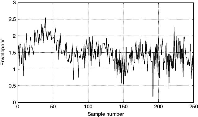
Figure 5.38 Fit to empirical data in Figure 5.37: (a) log-normal fit and (b) Weibull fit.

Following the estimation of , the hypothesis is rejected if it does not meet a certain confidence level , as given in:

5.40

For example, for a 95 % confidence level, . Using Equation (5.40) for the 250 data points in Figure 5.37, this gives an upper limit of . Comparing this upper limit with the values of in Figure 5.38 we see that the Weibull distribution meets the set criterion with whereas the log-normal distribution has to be rejected with .

5.10 Medium/Large-Scale Characterization

5.10.1 CDF Representation

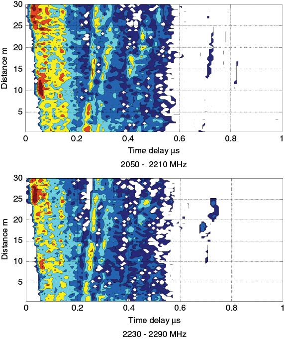
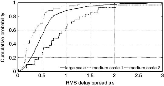
Medium- and large-scale characterization refers to measurements being performed over an area of either a few hundred metres (medium scale) or a large area extending to several hundred metres to kilometres, for example covering a city centre. These measurements can be either wideband or narrowband and can represent parameters such as RMS delay spread, path loss, coherent bandwidth, coherent time or coherent distance. An example of medium- and large-scale characterization of a dense urban environment is shown in Figure 5.39, which displays the city centre of Manchester with medium-scale routes numbered as 1–3 and 6–8 and the corresponding PDP collected along two of the routes (route 1 and 8) as a function of location with a 60 MHz bandwidth at 1950 MHz [9]. For wideband parameters the data set consisting of values computed over small-scale areas (location) are represented by a CDF, as illustrated in Figure 5.40 for the RMS delay spread values for two of the routes (medium scale 1 and 2) and for all the measurements covering 580 locations (large scale). Values corresponding to the 90 % or the median of the CDF are usually used as an indication of the percentage of locations that has a value less than the corresponding value on the x axis. For the example, in Figure 5.40 the median RMS delay spread values are 0.29 and 0.84 µs for the two medium-scale routes and 0.49 µs for the large-scale characterization. The values indicate that wide variations can occur from one route to the other and to obtain a more characteristic value of a large area it is necessary to obtain a large set of data.

Figure 5.39 (a) Map of city centre in Manchester with indicated routes and PDP along (b) route one and (c) route eight [9].

Source: Salous, S., and H. Gokalp, (2007), Medium and large scale characterisation of UMTS allocated frequency division duplex channels, IEEE Transaction on Vehicular Technology, 56(5), pp 2831–2843. Reproduced with permission IEEE.

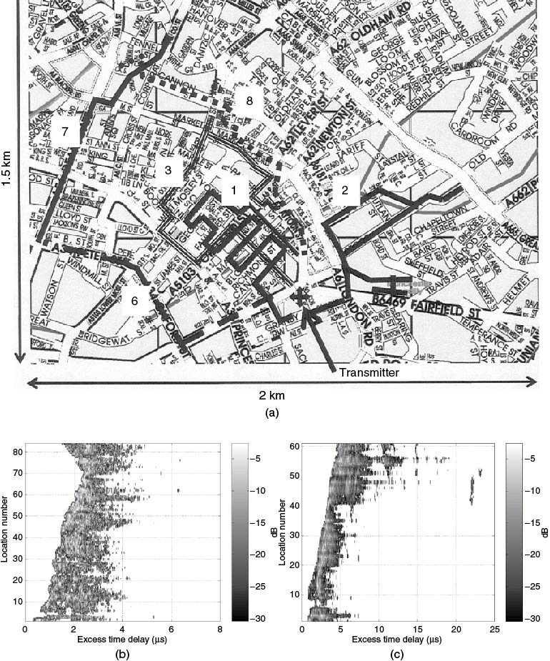
Figure 5.40 RMS delay spread cumulative distribution for two routes and for all the data set in the city centre of Manchester.

5.10.2 Estimation of Path Loss

Another parameter that can be extracted from wideband measurements is the path loss and its relationship to the RMS delay spread. Received signal power can be estimated from the calibrated PDPs by taking the sum of the power versus time delay, that is the magnitude square of the complex impulse response as in:

5.41

The calibration of the PDPs is obtained from back-to-back measurement where a known transmitted signal with P_cal (dBm) is fed to the receiver via direct connection with a short cable and the signal level at the ADC is recorded to identify the overall system gain G_Rcal. The area under the magnitude square of the complex impulse response of the system is computed as in Equation (5.41) and used as a reference in the calibration [24]. Thus for a transmitted power of P_T, transmitter antenna gain of G _T and receive antenna gain of G_R, the path loss P_L can be expressed as:

5.42a

where

5.42b

Analyzing the small-scale data to obtain the path loss over a large area as a function of distance gives a scatter plot. Using regression analysis that minimizes the mean square error gives the path loss coefficient n, as illustrated in Figure 5.41, where the mean path loss is given by:

5.43

where d_o is a reference distance usually taken as 1 m. This gives the path loss at the reference distance as in the following equation, which can be computed for the operating frequency:

5.44

Since path loss can be high close to the transmitter due to shadowing effects, the effect of distance can be eliminated by estimating the excess path loss, which is obtained by taking the difference between the measured path loss and the path loss computed from the regression curve. This gives the scatter plot in Figure 5.42, where positive values indicate a higher path loss and negative values indicate a lower path loss.

Figure 5.41 Scatter plot of path loss versus transmitter and receiver distance and regression fit giving a value of n = 2.56.

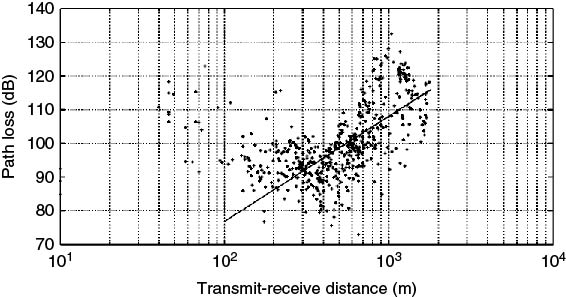
Figure 5.42 Scatter plot excess path loss versus transmitter and receiver distance.

Path loss measurements can also be performed using narrowband transmissions. Since in the narrowband case the signal suffers from fading due to the presence of multipath it is necessary to take measurements over a number of spatially separated points over fractions of a wavelength extending over 20–40 wavelengths. These are subsequently averaged in order to eliminate the fast fading. The average data are then used to extract the path loss coefficient as in the wideband case. Equally, excess path loss can be computed to estimate shadow fading. The measurements need to be calibrated for the gain of the receiver, antenna gain and cable losses. In Section 2.6 measurement-based path loss models that include correction factors for frequency, antenna height at the base station and at the receiver and antenna gain were briefly discussed.

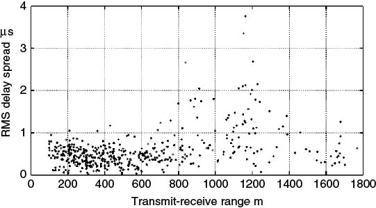
5.10.3 Relating RMS Delay Spread to Path Loss and Distance

Models relating RMS delay spread to shadowing and distance between the transmitter and receiver have been proposed in the literature. Using the computed RMS delay spread values scatter plot as a function of path loss or distance can be generated as in Figure 5.43 and regression analysis can be used to obtain a suitable relationship. For example, a model that relates the median RMS delay spread of an area () to distance and the median RMS delay spread at 1 km (T₁) is proposed in [25] and is given below, where ϵ has a value between 0.5 and 1 for terrains ranging from urban to mountainous with 0.5 for urban areas:

5.45

where d_max is the maximum radius of the area of measurements.

Figure 5.43 Scatter plot of RMS delay spread as a function of range.

To allow for different reference distances other than 1 km the model can be expressed as [9]:

5.46

The value of ϵ can then be estimated using the measured values of the RMS delay spread by taking a similar number of data points at different range intervals for the evaluation of the median to be used in Equation (5.46). For example, taking values at the ranges of 300, 500 and 700 m can be used to evaluate the coefficient for maximum ranges of 400, 600 and 800 m. For these distances the median RMS delay spread for the measurements reported in [9] were found to be 0.47, 0.42 and 0.49 µs, giving a value for ϵ equal to 0.56 for maximum distances of 600 and 800 m and 0.04 for maximum distances of 400 and 800 m. While the first value is close to the proposed 0.5 factor in [25], the second value is significantly smaller.

Similarly, analysis can be performed on the RMS delay spread as a function of path loss to obtain an empirical relationship for the uplink and downlink respectively for the UMTS measurements reported in [9]:

5.47a

5.47b

Since shadowing gives rise to a higher RMS delay spread, as can be seen in Figure 5.44a for two different routes, an alternative is to use the excess path loss as in the scatter plot in Figure 5.44b. Using the regression analysis from the path loss coefficient and substituting in Equations (5.47a) and (5.47b) give the relationships for the uplink and downlink of the UMTS FDD (frequency division duplex) bands respectively [9]:

5.48a

5.48b

Figure 5.44 (a) Path loss as a function of location and corresponding RMS delay spread for two different routes (a,c, route 1; b,d, route 2 in Figure 5.39a). (b) Scatter plot of RMS delay spread versus excess path loss [9].

Source: Salous, S., and H. Gokalp, (2007), Medium and large scale characterisation of UMTS allocated frequency division duplex channels, IEEE Transaction on Vehicular Technology, 56(5), pp 2831–2843. Reproduced with permission IEEE.

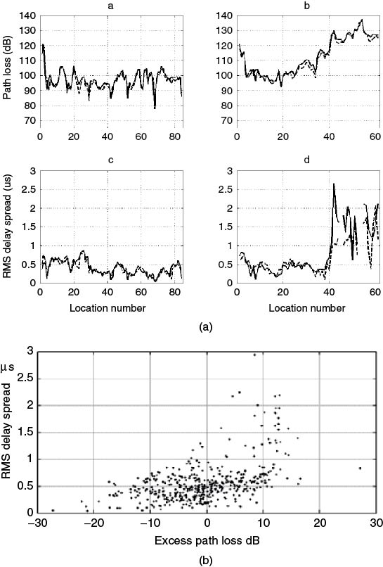
These relationships show that the RMS delay spread increases linearly with excess path loss but logarithmically with distance. The scatter plot of the RMS delay spread versus the excess path loss for the uplink shown in Figure 5.44b also indicates an exponential relationship between the RMS delay spread and the excess path loss. Thus, regression analysis can also be performed using the natural logarithm of delay spread in ns, excess path loss EP_L in dB and distance in m. The maximum difference between the exponential fit and Equations (5.48a) and (5.48b) is reported to be 80 ns [9].

An alternative is to use the overbound exponential model, which offers a simple model between the RMS delay spread, path loss and distance where the path loss is referenced to a 1 m separation between the transmitter and receiver [24]:

5.49

Expressing the RMS delay spread in nanoseconds and P_L(d) in dB a value of 0.065 for the coefficient is reported in [24] and for the data in Figure 5.45 the coefficient is equal to 0.039.

Figure 5.45 Scatter plot of RMS delay spread versus path loss overlaid with an exponential overbound.

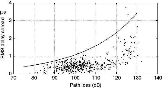
It is generally important in applying the coefficients derived from measurements to relate the model to the environment and to the experimental set-up such as antenna heights at the transmitter and at the deceiver and to whether the environment is a rural, suburban or dense urban environment. If the antenna height is low, as in picocells, then the Frensel zone breakpoint needs to be taken into account in the path loss coefficient model. Also the street orientation with respect to the transmitter and the presence of high-rise buildings affects the RMS delay spread, where heavily shadowed areas can give rise to a high RMS delay spread even if they are in the proximity of the transmitter and in faraway locations where the LOS is present this can lead to a low RMS delay spread.

5.10.4 Frequency Dependence of Channel Parameters

In Section 2.9.2.4 examples of PDPs illustrated the differences in the multipath structure as a function of frequency, particularly in heavily shadowed locations. These differences give rise to different estimates in the RMS delay spread and other small-scale channel parameters. Therefore estimates obtained with the same time delay resolution across a band of frequencies give variations in the CDFs. To study the frequency dependence of an RMS delay spread, it is necessary to transmit on multiple frequencies or to analyze the data with reduced resolution by subdividing the bandwidth into sections. For example, the 60 MHz bandwidth for the uplink and downlink of the UMTS band can be divided into 5 MHz sections for which CDFs can be generated for both medium-scale and large-scale areas, as shown in Figure 5.46 for a single route (a–b) and for all the routes (c–d of Figure 5.39a) where the horizontal lines indicate the variations across the 12 frequency sections. The figure shows that the frequency variations are less pronounced for the large-scale CDFs obtained from all of the routes than for medium-scale variations of a single route. This is expected because as more values are included in the data pool the random variations due to the measured environment are reduced. Scaling the 90 % values from the CDFs for each section gives the range of values of the variations as a function of frequency. This effect is illustrated in Figure 5.47, which gives the RMS delay spread for 10 different routes for the uplink and downlink analyzed with a 60 MHz bandwidth and with a 5 MHz bandwidth as indicated by the vertical lines, which show the range of variations across the 12 sections.

Figure 5.46 CDFs of RMS delay spread across the 12 frequency sections: (a,b) uplink and downlink for one route and (c,d) for all the routes. Horizontal lines indicate variations across the different frequency sections.

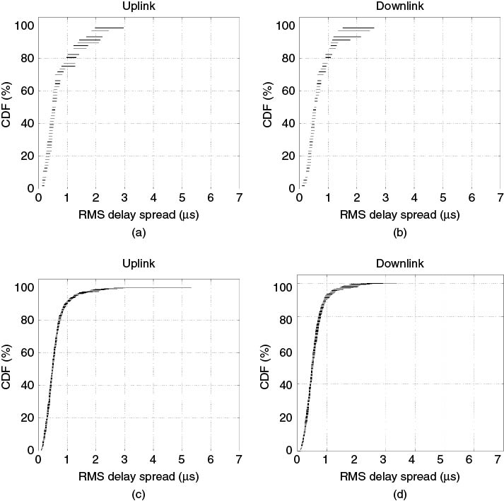
Figure 5.47 CDF values at 90 % of RMS delay spread as a function of route number for the uplink (solid line) and the downlink (dashed line); vertical lines indicate the variations across the 12 frequency sections [9]. Source: Salous, S., and H. Gokalp, (2007), Medium and large scale characterisation of UMTS allocated frequency division duplex channels, IEEE Transaction on Vehicular Technology, 56(5), pp 2831–2843. Reproduced with permission IEEE.

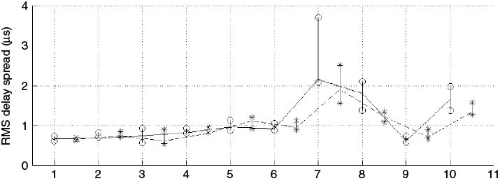
An alternative to the CDF is to present the difference of the channel parameters between two frequencies. For example for FDD systems the difference between the uplink and the downlink RMS delay spread can be represented by a PDF as in Figure 5.48 for both 60 MHz bandwidth resolution and 5 MHz bandwidth resolution for a medium-scale area. The figure shows that higher differences can be observed within the 5 MHz bandwidth resolution. Appropriate system design therefore requires measurements with the system bandwidth to obtain more accurate channel parameters.

Figure 5.48 PDF of the difference in RMS delay spread between the uplink and downlink for a medium-scale area (a) with a 60 MHz bandwidth resolution and (b) with a 5 MHz bandwidth resolution [9]. Source: Salous, S., and H. Gokalp, (2007), Medium and large scale characterisation of UMTS allocated frequency division duplex channels, IEEE Transaction on Vehicular Technology, 56(5), pp 2831–2843. Reproduced with permission IEEE.

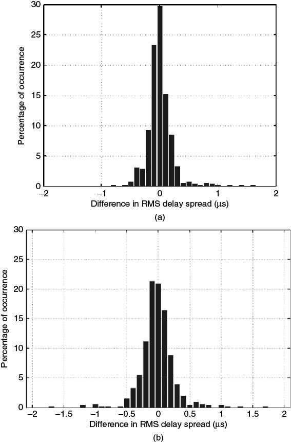
5.11 Multiple Antenna Array Processing for Estimation of Direction of Arrival

Systems with antenna arrays have many applications, which in addition to wireless communication include radar, radio astronomy, sonar, seismology, tomography, detection and localization of sources, tracking the instantaneous positions of sources and enhancing the quality of the received signal by spatial filtering interference and noise.

Depending on the application, antenna array systems can be deployed in three configurations: single input–multiple output (SIMO), multiple input–single output (MISO) and MIMO. SIMO data can be analyzed to estimate the direction of arrival (DOA) of the different sources and track their movement or it can be used to estimate antenna diversity gain to enhance the received SNR and data rates. MISO antenna arrays can be used for transmit diversity or to form different beam patterns for directional transmission, known as smart antenna transmission. MIMO antenna arrays enable a wide range of studies, which include diversity gain at the transmitter and at the receiver, estimation of the direction of departure (DOD) and DOA of rays connecting the transmitter to the receiver and enhancement of MIMO capacity.

To estimate the DOA and DOD using multiple array elements a number of processing techniques have been developed over the years [26], starting in 1945 with conventional beam forming. This was followed in 1967 by the maximum entropy (ME) method developed by Burg [27] and in 1969 by Capon's maximum likelihood (ML) method [28]. In 1973 Pisarenko correctly exploited the structure of the data models using harmonic retrieval [29] and in the period 1980–1981 Bienvenu and Kopp [30] and independently Schmidt [31] introduced signal subspace methods. They were the first to correctly exploit the measurement model in the case of sensor arrays of arbitrary form. This led to the introduction of the ‘MUSIC’ algorithm, which requires full knowledge of the antenna manifold, that is the gain and phase pattern distribution of the antenna and the array geometry. In 1989 Roy [32, 33] introduced the ESPRIT, the technique that revolutionized sensor array processing for a number of reasons. Firstly, it does not require knowledge of the antenna directional patterns, secondly, compared to MUSIC it is more robust to array perturbation and requires less computations and, thirdly, ESPRIT estimates are less biased for finite data lengths. A variant of EPSRIT called unitary ESPRIT was later developed to deal with centrosymmetric array geometries [34].

In 1994 Fessler and Hero [35] proposed the SAGE, a technique that uses the principle of ML estimation criterion, which since then has been used for joint parameter estimation such as delay and angle estimation in time-invariant environments or joint delay, angle and Doppler frequency estimation in time-variant environments [36, 37].

These various techniques can be grouped into three classes as illustrated in Figure 5.49:

• Spectral-based estimation techniques.
• Parametric estimation techniques or parametric subspace estimation (PSE).
• Joint parametric estimation (JPE) techniques.

Figure 5.49 Classification of array processing techniques.

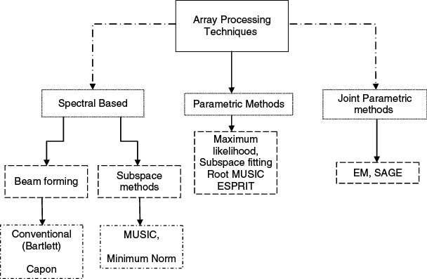
In this section we start with the theoretical problem for the estimation of the DOA followed by investigation of the various array processing techniques.

5.11.1 Theoretical Considerations for the Estimation of Direction of Arrival

The problem to be solved here is depicted in Figure 5.50 where an array of M antennas receives waves from P sources. These sources are assumed to be independent and the receiver attempts to identify their directions of arrival. In order to solve this problem a number of assumptions are made, in particular the narrowband assumption of the received signal. Two main functions are needed in order to solve this problem and these are the steering vector of the array and the covariance matrix. In this section we start by listing the basic assumptions and the implications of the narrowband assumption, followed by analysis of the linear array and the uniform circular array (UCA) to give examples of the steering vector. We then define the spatial covariance matrix, which forms the foundation of analysis of the DOA.

Figure 5.50 Illustration of waves from P sources impinging on an M element array.

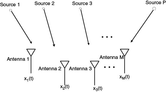
5.11.1.1 Basic Assumptions

A number of assumptions are usually made in solving this problem:

1. The transmission medium is nondispersive and isotropic.

2. The sources of the impinging signals are in the far field, which means that the radius of propagation is much larger than the array largest dimension; thus, the arriving waves can be considered plane waves with constant phase.

3. The noise samples are assumed to be uncorrelated with the source signal.

4. The complex radiation pattern (magnitude and phase) of the antenna array is assumed to be known for all angles.

5. The number of sources P is less than the number of antenna elements M, that is .

6. The source signal is narrowband with bandwidth , where f_c is the carrier frequency and , where D refers to the largest dimension of the array and is the speed of light. This implies that all the frequency components of the signal as they propagate over the length of the array give rise to similar signal strengths and undergo the same phase shift; thereby the time delay difference of arrival at the array elements can be represented by a phase shift at the carrier frequency of the incident wave. The narrowband case also implies that the complex response of the antennas is not frequency dependent across the bandwidth of the signal. This is generally satisfied for most communication systems but is not applicable for ultra-wideband signals. In this section we restrict the analysis to the narrowband case.

Referring to Figure 5.50, the received signal at any instant in time consists of M samples, which represent a spatial snapshot of the impinging wave. Sampling the output of the antenna array at instants , where is the number of the snapshots extracted for processing, forms the output vector process x(t), which represents a temporal space vector of size N_o × M. It is assumed that the signal from a single source impinging on the array can be represented by:

5.50

where and are the modulated signal's amplitude and phase respectively and is the angular carrier frequency. For a small time delay equal to the relationships in Equations (5.51) follow from the narrowband assumption:

5.51

Using the complex analytical signal representation of the received signal can be expressed as:

5.52

Multiplying Equation (5.52) by gives the baseband signal .

The DOA information is contained in the time delays of the propagating wave between the different antenna elements. The narrowband assumption implies that the complex envelope of the received signal as it propagates between the different antenna elements is given by:

5.53

5.11.1.2 Linear Array Analysis

Taking the example of the linear array in Figure 5.51 and assuming that the first antenna element designated as number 0 is the reference antenna, the received signals on consecutive antennas are delayed in time by:

5.54

and θ is the angle relative to the broadside of the array, that is the line perpendicular to the array line as illustrated in Figure 5.51.

Figure 5.51 Linear array illustrating the direction of arrival.

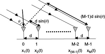
Each received signal is also multiplied by the gain factor of the array element and then demodulated. Taking the noise into account, this gives rise to the signal at the mth antenna output to be of the form given by:

5.55

For M antenna elements, the received signal can be written in vector form as:

5.56

where and is additive white Gaussian noise and:

In the narrowband assumption we also evaluate the complex responses of each antenna in the array at the centre angular frequency of the signal. This gives the complex array as:

5.57

Assuming identical (uniform) antenna array elements and a homogeneous array where all the elements are positioned in an identical manner, this reduces to:

5.58

is called the steering vector for that particular DOA and substituting for and the wavenumber k = 2π/λ we get:

5.59

The uniform linear array represents a simple implementation and is widely used. However, two issues need to be considered in the design and application of such an array: (i) the back–front ambiguity and (ii) the interelement spacing. Referring to Figure 5.52, the back–front ambiguity can be explained by the fact that a wave arriving from an angle θ would give rise to the same phase difference between elements regardless of whether it is above or below the array. Therefore, an array consisting of omnidirectional elements can only distinguish sources arriving between −90 and 90° with respect to the broadside. Using directive antennas this ambiguity can be eliminated but would then require two sets of elements to cover both directions.

Figure 5.52 Illustration of the back–front ambiguity of the linear array.

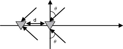
The interelement separation d has to be restricted to avoid spatial aliasing. This follows from the periodicity of sin θ, where an additional rotation by π gives the same phase difference between two adjacent antennas. Assuming that the DOA is 90° and restricting the phase to π radians gives the condition 2πd/λ < π or, alternatively, d < λ/2.

For P sources the received signal vector is the sum from all the sources and can be expressed as:

5.60

where x(t) is the M × 1 signal vector, s(t) is the P × 1 source signal vector, ) and n(t) is the M × 1 noise vector. A(θ) is the M × P steering matrix consisting of P array steering vectors, a(θ_i), each of dimension M × 1 expressed as:

5.61

Equation (5.60) consists of P steering vectors for each incoming wave, which for a ULA is the Vandermonde matrix given by:

5.62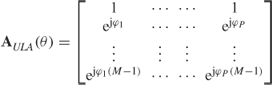

where

5.11.1.3 Circular Array Analysis

The back–front ambiguity of the linear array can be resolved by using two-dimensional arrays such as the circular array shown in Figure 5.53. This array resolves the ambiguity in the azimuth plane and is capable of estimating the angular information in elevation, with up/down ambiguity similar to the uniform linear array (ULA). For full resolution in azimuth and in elevation it is necessary to have a stacked array. For an array configuration that permits the estimation of both the azimuth angle θ and the elevation angle φ, it is assumed that the azimuth angle θ is measured from the y axis in the clockwise direction and the elevation angle φ is measured down from the z axis. An alternative description for the DOA is then formed by the direction cosines and with respect to the axes respectively. The array steering vector can then be expressed as [38]:

where

5.63

Figure 5.53 Illustration of the uniform circular array.

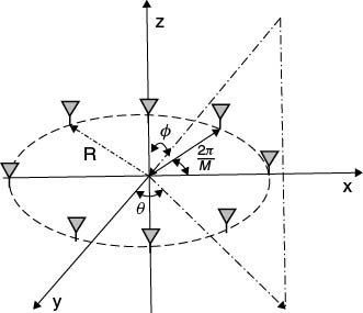
is the Hadamard product.

Taking the UCA shown in Figure 5.53 with M elements as an example, the angle displacement with respect to the centre of the array is equal to , giving the following steering vector:

5.64

where and is the vector containing the angle parameters of the signal.

For waves arriving in azimuth only the steering vector of the UCA for φ = 90° reduces to:

5.65

Array manifolds can be extracted either analytically from an exact knowledge of the antenna directivity patterns and the array geometry or experimentally by taking calibration measurements of the array.

5.11.1.4 Covariance Matrix

Since the DOA parameter is a spatial parameter, most techniques attempt to approximate the exact spatial covariance matrix R of the measured data. This matrix has the form given by [26]:

5.66

where denotes the statistical expectation, H is the Hermetian transpose operator, is the array manifold matrix, is the signal covariance matrix and is the noise covariance matrix. Equation (5.66) follows from the assumption that all the noise sources at the different sensors have zero mean and equal variance and are uncorrelated with each other and with the signal. In the event of additive man-made noise where the assumption of white noise does not hold, the output vectors from the array can be prewhitened by premultiplying by the square root of the inverse of the noise covariance matrix N.

The rank of the matrix S depends on whether the received signals are incoherent; that is none of the received signals is linearly related to or is a linear combination of the other signals. If S is of full rank and nonsingular this simplifies the estimation problem considerably. In the context of channel characterization the multipath components are considered coherent signals since they are scaled and delayed versions of each other.

The spatial covariance matrix R can be eigen-decomposed into where is the diagonal matrix in the following equation, which contains the eigenvalues and is the unitary matrix defined as :

5.67

Since P < M the matrix can be further decomposed into two subspaces, the signal subspace and the noise subspace , which gives the expression for the covariance matrix:

5.68a

5.68b

In real array measurements the covariance matrices are unknown and can only be estimated from a finite amount of measurement snapshots N_o, which also means that only an estimate of the signal subspace can be obtained. The standard method of obtaining such an estimate is by forming the matrix in Equation (5.69):

5.69

5.11.2 Spectral-Based Array Processing Techniques

5.11.2.1 Beam Forming

The first and most straightforward spectral-based method is known as beam forming. Historically beam forming or spatial filtering was first developed during the Second World War (1945) [26] and is based on the idea that the antenna array is steered to one direction at a time. The direction that gives the maximum power is the DOA of the wave. Steering the array response can be achieved by forming a linear combination of the antenna outputs. In this case each received signal is weighted by w and the weighted components are added to form the output signal as shown in Figure 5.54.

Figure 5.54 Illustration of the beam forming concept.

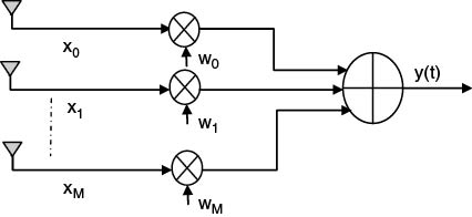
A measure of the average output power over snapshots is then formed as indicated in:

5.70

where is the covariance matrix defined in Equation (5.69).

Different beam forming approaches differ by the choice of the weighting vector w. Two commonly known beam forming methods briefly described in this section are the Bartlett method and the Capon method. Both techniques require a one-dimensional (1D) search for the estimation of the DOA in azimuth and they are incapable of dealing with coherent signals.

5.11.2.2 Conventional Beam Forming (Bartlett Method)

Conventional beam forming is based on maximizing the received power in a given direction θ provided that the noise is spatially white. This condition is expressed by:

5.71

A solution that satisfies the maximization problem in Equation (5.71) is given by:

5.72

The weights compensate for the different time delays of the signal along the array to combine their contributions to give maximum power from the direction θ and can be viewed as a spatial matched filter to the incoming signal. Substituting the weighting vector in Equation (5.71), a spectrum-like function is formed as:

5.73

Inserting the steering vector of a ULA in Equation (5.73) and noting that , the denominator becomes equal to M and the expression for the power becomes a spatial Fourier transform [26]. Similar to spectral analysis, the Bartlett beamformer suffers from limited resolution, which is restricted by the size of the array to .

5.11.2.3 Capon Method

Capon's beamformer, also known as the minimum variance distortionless response filter in the acoustic literature, attempts to reduce noise and spectral leakage from signals arriving from unwanted angles while maintaining fixed gain in the wanted direction θ by optimizing:

5.74

The optimal weighting vector for Capon's beamformer is given by:

5.75

which results in the ‘spatial spectrum’ given in:

5.76

Capon's beamformer tries to concentrate the received energy from all the antennas in the array in the direction of interest θ and hence can be viewed as a spatial bandpass filter [26]. However, Capon's method is limited by the physical size of the array and the SNR, η. This resolution threshold when assuming a perfect estimate of the covariance matrix is equal to [39].

5.11.2.4 Subspace-Based Methods

The subspace-based methods rely on the decomposition of the covariance matrix into signal subspace and noise subspace using eigenvalue decomposition (EVD) as in Equations (5.68a) and (5.68b), that is [26]. Since it is assumed that the signal and noise are uncorrelated, the projection of the signal vector for a given source with a given DOA on to the noise space will be very small or equal to zero:

5.77

For unambiguous estimation of the DOA it is assumed that the array steering vectors are independent to provide a full rank matrix.

5.11.2.5 MUSIC

The solution that satisfies Equation (5.77) gives the MUSIC ‘spatial spectrum’:

5.78

The spectrum, also known as the pseudo-spectrum, exhibits maxima in the vicinity of the true DOAs where the P largest peaks in the MUSIC spectrum correspond to the P estimated angles of arrival.

An alternative to first estimating the covariance matrix and then performing the EVD is to perform singular value decomposition (SVD) directly on the data matrix using each of the columns of the data matrix representing each measurement snapshot and each of the M rows representing an antenna and taking the P left singular vectors corresponding to the P largest singular values [33]. SVD is useful in the case of ill-conditioned matrices (matrices whose elements are very small numbers).

The computational cost of the full SVD of X can be considerably higher than the corresponding cost of a simple EVD of . However, a number of efficient algorithms are available for the SVD such as the rank-revealing QR decomposition [40], the URV decomposition [41] and Schur-type methods [42].

For a large number of snapshots and high SNR the MUSIC algorithm estimates are highly accurate. However, the algorithm has a number of shortcomings: (i) poor resolution in low SNR and with small antenna array calibration errors, (ii) it does not solve the problem of coherent sources as it relies on having a full rank matrix and (iii) in the case of joint parameter estimation (multidimensional searches of the spectrum) the computational cost increases exponentially.

The problem of small amounts of samples, low SNR and high correlation of signals can be partly circumvented by application of a nonuniform weighting factor in the MUSIC pseudo-spectrum as given in:

5.79

where

Although this weighting improves the resolution capability it does, however, increase the variance of the estimates.

In the case of linear arrays and two coherent sources, forward–backward averaging can be used to decorrelate the signals. For the general case with more coherent sources spatial smoothing can be applied to decorrelate the signals and thus increase the rank of the covariance matrix. This is achieved by subdividing an array of M elements into subarrays of p elements each, as shown in Figure 5.55, and assuming that all the subarrays have identical steering vectors (translational invariance property), the resultant K estimates (K = M – p + 1) are averaged to obtain the covariance matrix [26, p. 76]:

where

5.80

Figure 5.55 Illustration of an array subdivision for spatial smoothing.

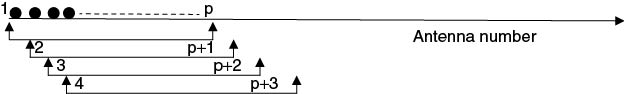
For each additional subarray the rank of the matrix increases by one. This is achieved at the expense of a reduced aperture of the array since now the effective size of the array is that of the subarray. For other array geometries, such as, for example, the circular array, a transformation that takes into account the geometry has to be applied to the data prior to spatial smoothing.

MUSIC can be used as an alternative method for the estimation of the spectrum of a signal as illustrated in Figure 5.56, where the signal consists of three sinusoids in additive white Gaussian noise. The spectrum is obtained by a 50 % overlap of the samples and using a rectangular window.

Figure 5.56 Spectrum analysis using a MUSIC pseudo-spectrum.

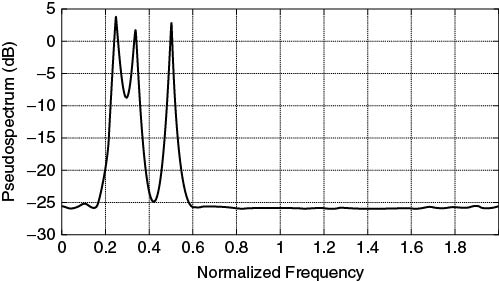
5.11.3 Parametric Methods

The limitation of spectral-based methods in identifying coherent sources can be resolved by using parametric methods. This, however, is achieved at the expense of higher computation complexity.

Parametric techniques include ML, a variation of MUSIC named Root-MUSIC, ESPRIT and its useful variation Unitary-ESPRIT. While the various ML techniques are applicable to arbitrary array geometries, the other methods require either a ULA configuration or a suitable transformation to take into account arbitrary array geometry. Here we give a brief description of ML, Root-MUSIC and ESPRIT.

5.11.3.1 Maximum Likelihood

The ML method is based on maximizing the ‘likelihood function’, which is based on a PDF f for a given distribution. Mathematically this is given by:

5.81

where is the PDF, x_i represent the data and are the parameters to be estimated.

For mathematical convenience the natural logarithm of Equation (5.81) is used to generate the log-likelihood function:

5.82

Subsequently, the parameters that maximize this function are estimated by taking the partial derivative with respect to each parameter and setting it equal to zero as in:

5.83

To apply the ML method for DOA estimation a signal model and a noise model need to be defined. Two models are used for the signal: one model assumes that the signal waveforms are unknown, arbitrary but deterministic, leading to the deterministic maximum likelihood (DML) technique; the second model assumes that the signal waveforms are Gaussian random processes, leading to the stochastic maximum likelihood (SML) technique [26]. In both cases, the noise is modelled as a stationary white Gaussian process and is also assumed to be circularly symmetric. This means that the real and imaginary parts are identically distributed and the cross covariance has a skew symmetry defined by [26]:

5.84

This means that the observation vector x(t) can also be considered as circularly symmetric and temporally white Gaussian random process.

Using the ML estimation for each parameter with the given PDFs for the signal and noise models, in the case of DML the DOA estimates are obtained by solving the minimization problem given by:

5.85

The method can cope with highly correlated or even coherent signals and provides consistent estimates.

In the case of SML the criterion is more complicated as the following equation indicates:

5.86

where

5.87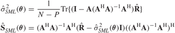

When a large number of snapshots is available, the SML estimates are more accurate than those of the DML, in particular for a small number of antennas M, low SNR and strong correlation among signals.

5.11.3.2 Root-MUSIC

For the case of a ULA an efficient and simplified parametric MUSIC technique called Root MUSIC, introduced in 1983 by Barabell [43], can be used. Here the antenna steering vector of the ULA is expressed as a polynomial with respect to z, , which has P zeros at z = and are the phase shifts between the antenna elements in the array [26].

This essentially removes the DOA search required in the MUSIC method. Instead, the DOA estimates correspond to the 2(M – 1) roots of the symmetrical polynomial defined as:

5.88

The phases of the P largest roots of the polynomial give the desired DOAs, as in:

5.89

For small sets of data Root-MUSIC performs significantly better than MUSIC.

5.11.3.3 ESPRIT

ESPRIT is a general subspace-based technique that can be applied to any array that exhibits the property of rotational or shift invariance. This property exists if the array can be subdivided into two subarrays displaced by a known translation . The DOAs are then defined relative to the normal of this translation [39]. To solve for the DOA the gain and phase patterns of each antenna element in the subarrays do not need to be known and nor do they need to have the same radiation pattern. The ESPRIT concept can also be extended to geometries with overlapping elements between subarrays as shown in Figure 5.57 for both overlapping and nonoverlapping subarrays.

Figure 5.57 (a) Overlapping subarrays and (b) nonoverlapping subarrays.

Each subarray configuration can be described by a pair of matrices and , which select the corresponding elements of the snapshot for each subarray. For the case of maximum overlap as in Figure 5.57a, these selection matrices take the form given by:

5.90

Taking the case of nonoverlapping ULA subarrays, each with M/2 antenna elements and a displacement vector , the Vandermonde structure of the global ULA steering matrix can be split into two matrices A₁ and A₂ using the selection matrices such that:

5.91

Matrix is a unitary matrix with diagonal elements representing the phase delays of the signals between the corresponding antennas of each subarray given as:

5.92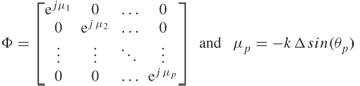

Hence, the DOA estimation problem in the case of ESPRIT reduces to finding the matrix where the diagonal elements are given by:

5.93

Taking the output vectors of the two subarrays x₁(t) and x₂(t) as:

and inserting the selection matrices, the whole array output can be expressed in the compact form given in:

5.94

The signal subspace estimation can then be obtained either via EVD on the overall covariance matrix or via SVD of the complete array of the data matrix X. The matrix can be decomposed into and by using the selection matrices as:

5.95

where the matrix T is unique and nonsingular. The diagonal elements of are obtained from the second key equation of the ESPRIT algorithm [33]:

5.96

where and have the same eigenvalues, which for i = 1, …, P are denoted by . The operator rotates into by applying the relationship:

5.97

which is known as the invariance equation.

Two techniques based on the least squares (LS) or the total least squares (TLS) criteria are usually used to solve Equation (5.97). In the case of a high SNR the difference in performance between the two criteria is negligible. However, in the case of a small number of snapshots or low SNR, TLS-ESPRIT is more robust, yielding unbiased and strongly consistent estimates [44].

Using the TLS method, is solved via SVD of the matrix to give the solution:

5.98

For a ULA the angles of arrival , of the P impinging signals can then be estimated from:

5.99

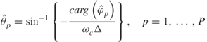
where is the pth eigenvalue of the solution matrix in Equation (5.98). For array structures with multiple invariances it is not possible to have a unique decomposition of matrix into and . In this case a variation of ESPRIT called multiple invariance ESPRIT can be used [45].

In summary, the steps for the computation of the ESPRIT algorithm for the case of a ULA matrix are:

1. Perform EVD on the complete array of the estimated covariance matrix or SVD on the complete data matrix and estimate the signal subspace .

2. Split the signal subspace into and using the selection matrices and .

3. Solve the set of equations by means of either LS or TLS.

4. Compute the eigenvalues of and derive the DOA estimates according to Equation (5.99).

ESPRIT has the advantage of offering high accuracy at a small computational cost, since no numerical search is required and the final solution is in closed form. However, due to practical constraints, the ESPRIT method is prone to more estimation errors than the ML method, which inherently exploits the full antenna model and not just the translation. A variant of ESPRIT named unitary ESPRIT provides a reliability test for the estimates that can result from a false estimate of the number of impinging signals , the absence of a signal (noise only case), antenna array imperfections and a low SNR. Using forward–backward averaging, unitary ESPRIT also deals with coherent sources.

5.11.4 Joint Parametric Techniques

In many applications, the DOA is not the only parameter of interest. For example, in radio channel characterization or radar, Doppler information as well as the time of arrival of the signal can be important parameters. In such applications it would be beneficial if all of these parameters could be estimated without the application of different algorithms. Such algorithms are termed joint parametric and here we discuss the SAGE maximization algorithm, SAGE. as an example. We start off by briefly describing the expectation maximization (EM) principle that forms the basis for SAGE and then discuss the application of SAGE to radio channel characterization.

5.11.4.1 Expectation Maximization (EM) Algorithm

EM is an iterative method that attempts to estimate a vector of unknown parameters from observed measurements by alternating between the estimation step (E-step) and the maximization step (M-step). The measured data set x(t) has a given statistical model with latent variables (hidden or unobserved variables) y(t), with a vector of unknown parameters θ and a likelihood function . EM computes the maximum likelihood estimate (MLE) or the maximum a posteriori (MAP) of the model parameters from the marginal likelihood function:

5.100

In the E-step, the expected value of the log-likelihood function is computed from:

5.101

This is followed by the M-step, which finds the parameters that maximize the quantity in:

5.102

In summary, the steps in the EM algorithm consist of:

The EM algorithm simultaneously maximizes the expectation with respect to all the unknown parameters. The simultaneous updating used in the classical EM algorithm leads to slow convergence and a difficult maximization step. To speed up the procedure, the SAGE algorithm, which sequentially updates the parameters in small groups, was proposed by Fessler and Hero [35].

5.11.4.2 EM Solution for Parameter Estimation in a Multipath Environment

Figure 5.58 displays the multipath signal model where the received signal x(t) at each sensor is the sum of P independent multipath components, each corrupted by independent additive white Gaussian noise to give y_p(t). Thus the received signal is given by:

5.103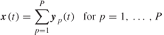

Figure 5.58 Multipath signal model [36].

Source: Fleury B. H., Tschudin M., Heddergott R., Dahlhaus D., Pedersen K. I., (1999), Channel parameter estimation in mobile radio environments using the SAGE algorithm, IEEE Journal on selected areas in communications, vol. 17(3), pp. 434–449. Reproduced with permission IEEE.

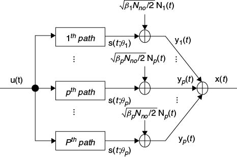
where

5.104

The N-dimensional vectors, N₁(t),…, N_p(t), are independent complex Gaussian white noise vectors, N_no is a positive constant and the parameters in the noise vectors are positive and satisfy . The signal represents the baseband signal for the pth multipath component with a parameter vector . In a multipath environment a number of parameters can be included and here as an example we consider the parameter vector , which gives the time delay, DOA in the azimuth plane, Doppler shift and complex weight respectively.

Thus the baseband signal of the pth multipath component is represented by:

5.105

where .

In the model the transmitted signal u(t) consists of a periodic repetition of impulses or can consist of a periodic pseudo-noise (PN) sequence to exploit the processing gain of a spread spectrum signal.

Assuming an array with M sensors, the overall received signal vector x(t) is given by and represents the measured incomplete data where represents the hidden or complete data. The unknowns associated with all the P paths then form the matrix .

5.11.4.3 EM Solution

Given the received vector x(t) sampled over an observation time and P uncorrelated multipath components, the problem to solve is to estimate the set of unknown parameters for each multipath component, . To apply the EM algorithm we need the log-likelihood function of given x(t) over . For independent vectors the log-likelihood function of each multipath parameter vector is given by [36]:

5.106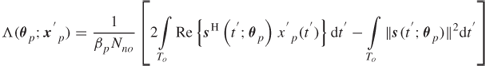

where denotes the norm of the argument and the MLE of for the observation is as given in:

5.107

The estimation step (E step) of the algorithm aims to estimate of the hidden data , conditioned to a particular observation as in:

5.108

The first term of Equation (5.108) is the contribution of the pth signal assuming that and the second term is an estimate of the noise assuming that .

The maximization step (M step) reestimates the vector from the estimate based on:

5.109

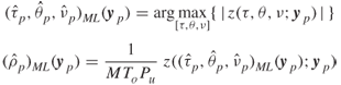
where the correlation function:

In Equation (5.109) the factor is the power in the signal and the factor gives the total energy collected over all the antennas in the array.

For any initial value, for example , the EM algorithm iterates by executing the two steps (E and M steps) and creates a sequence of estimates . The iteration process is stopped as soon as the difference between the estimates returned within two consecutive iterations is less than a predefined threshold. Using the uncorrelated property of the paths the algorithm splits the optimization process of joint estimation of P signals into P separate optimization problems.

5.11.4.4 SAGE Algorithm

The general form of the SAGE algorithm was initially derived in [35] and its main feature is the fast convergence to the desirable estimates. The algorithm finds the MLE estimates in Equation (5.109) sequentially. This is achieved by iteratively solving for the parameters of each path individually and estimating its contribution to the full measured vector x(t). The parameters are estimated by converting the multiparameter optimization problem for each multipath component into separate one-dimensional optimizations. For the example of the 3P model employed here, it subdivides the parameter set into three separate two-dimensional subsets, namely , and ; then since the complex amplitude can be expressed as a function of the other three parameters, the initial complicated optimization procedure is now split into 3 P separate one-dimensional optimizations. In short, the SAGE algorithm can be presented in mathematical notation as:

Expectation step with parallel interference cancellation

Maximization step using the coordinate-wise updating procedure[36], which states that if is the updated parameter estimates and is the previous estimate the procedure performs the following consecutive steps:

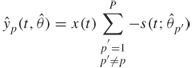
5.110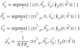

Figure 5.59 Signal flow graph of the SAGE algorithm ([36], Figure 5).

Source: Fleury B. H., Tschudin M., Heddergott R., Dahlhaus D., Pedersen K. I., (1999), Channel parameter estimation in mobile radio environments using the SAGE algorithm, IEEE Journal on selected areas in communications, vol. 17(3), pp. 434–449. Reproduced with permission IEEE.

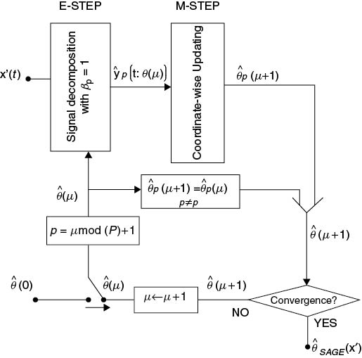
where

Figure 5.59 displays the flow graph of the SAGE algorithm where one iteration cycle refers to updating all the P signals.

5.12 Practical Considerations of DOA Estimation

In performing DOA studies the aim is to select a suitable antenna array configuration that allows adequate detection of impinging waves, good resolution and high accuracy of estimates. In addition antenna calibration files are also needed for the steering vector in the parameter estimation algorithm. In this section we discuss the various issues of antenna array selection and calibration and give examples of measured antenna responses and estimation of the angle of arrival.

5.12.1 Choice of Antenna Array

Antenna arrays can be either homogeneous or heterogeneous, where a homogeneous antenna array is defined as an array composed of the same type of antenna elements all oriented in the same direction regardless of the geometry of the array [46] as sketched in Figure 5.69a for a UCA. Comparison of homogeneous arrays set up in a linear, circular, Y, X, dual-ring or spiral geometries shows the following properties [47]:

In contrast, a heterogeneous antenna array can either have (i) different types of antenna elements [48, 49] or (ii) the same type of antenna elements with different orientations as illustrated in Figure 5.60b [46, 50]. For example, the circular uniform beam array (CUBA), the x-y-z antenna array and the Giselle antenna arrays in Sections 3.13.6 and 3.14.2 represent heterogeneous arrays consisting of identical elements with different orientations. The difference in orientation reduces the correlation between the elements and gives a higher MIMO capacity. Heterogeneous arrays can also be used in the estimation of DOA and again have a particular advantage in HF where spatial separation of elements is not practical. Figure 5.60c shows an eight element array used in an SIMO configuration in the HF band for DOA estimation [46, 48].

Figure 5.60 (a) Homogeneous circular array, (b) heterogeneous circular array and (c) eight collocated element heterogeneous arrays constructed from different antenna elements [49].

Source: Oger, M., F. Marie, D. Lemur, G. Le Bouter, Y. Erhel, and L. Bertel (2006), A method to calibrate HF receiving antenna arrays. 10th International Conference on Ionospheric Radio Systems and Techniques (IRST 2006), Inst. of Eng. and Technol., London. Reproduced with permission from IET.

A heterogeneous array used for DOA in the UHF band is the CUBA topology as in Figure 5.61a, which shows an octagonal arrangement of an eight element array with 45° per sector to provide 360° coverage in azimuth [52]. For such an array, extensive numerical simulations show that the optimum radius to minimize the probability of parameter estimation outliers is given by [51]:

5.111

where M is the number of antenna elements in the array. For an eight element array this results in a radius equal to half the wavelength. For operating at 2.3 GHz, this gives a radius equal to 65 mm, which requires a stacked configuration as shown in Figure 5.61b [52].

Figure 5.61 (a) Configuration of CUBA with eight elements providing 360° coverage and (b) a realized stacked array [52].

Source: Abdalla M., Feeney S.M., Salous, S., and Lewenz R., (2010), Design and calibration of circular uniform beam array for wideband channel characterisation. IET Microwave Antennas Propag., Vol. 4, Iss. 1, pp. 43–53 43, doi: 10.1049/iet-map.2008.0273. Reproduced with permission of IET.

Another aspect to consider in array element design is the polarization. For DOA estimation, vertically polarized patch antenna elements are considered to have good resolution in the presence of coherent sources [51]. Figure 5.62 shows an example of a vertically polarized directional array element realized with dual-arm series fed strip dipoles with ground plane reflectors to restrict the radiation pattern to the end-fire direction [52]. The arms are printed on opposite sides of an electrically thin substrate (relative permittivity ϵ_r = 2.2), connected through a wideband Wilkinson power combiner/splitter including a shaped ground conductor. The spacing D used between the two elements is 65 mm, with the reflector width w_c = 120 mm, the arm length L_c = 60 mm and φ = 30°. The use of two arms enables a phase shifter to be introduced to steer the beam of the element.

Figure 5.62 (a) Strip dipole with a dual arm configuration and (b) a realized antenna element [52].

Source: Abdalla M., Feeney S.M., Salous, S., and Lewenz R., (2010), Design and calibration of circular uniform beam array for wideband channel characterisation. IET Microwave Antennas Propag., Vol. 4, Iss. 1, pp. 43–53 43, doi: 10.1049/iet-map.2008.0273. Reproduced with permission of IET.

5.12.2 Array Calibration

Array calibration consists of two stages:

• Calibration of the single element to identify its performance against the theoretical design or the simulated results from antenna software packages.
• Calibration of the overall array since the individual elements once placed in the array will have their performance modified due to mutual coupling. Mutual coupling arises from the radiation of each element inducing currents in the neighbouring elements. These are then either fed back into the system or radiated into the far field, thus changing the radiation pattern from that of the isolated element pattern. The overall current on each array element is therefore the sum due to its own excitation plus all the contributions from the various coupling sources. This mutual coupling can affect the estimation of the channel parameters using high resolution algorithms [53].

5.12.2.1 Calibration of Single Antenna Element

5.12.2.1.1 Measurements of Input Impedance, Input Return Loss, VSWR and Smith Chart

These can be performed using a vector network analyzer set up to measure the single port characteristics, for example S₁₁ for return loss, VSWR, Smith chart and input impedance. Before measuring the antenna characteristics the network analyzer should be calibrated to correct for any systematic errors due to the adaptors, cables and other imperfections of the measurement system. This is achieved using the calibration unit for various tests, which include short, open and load tests.

5.12.2.1.2 Measurements of Radiation Pattern

The radiation pattern measurements can be performed using either a network analyzer or custom hardware in conjunction with a turntable and data acquisition unit to measure the azimuthal radiation pattern in an anechoic environment. For measurements in the elevation angle, the turntable is turned in discrete angular steps to cover the 360^o and a snapshot is recorded. The procedure is repeated for all the required elevation angles to obtain the three-dimensional radiation pattern. A network analyzer set-up is shown in Figure 5.63 with a three-dimensional radiation pattern of a wideband discone antenna measured at 2.4 GHz where the radiation strength is defined by the intensity of the colour.

Figure 5.63 (a) Network analyzer set up for measuring the radiation pattern and (b) a measured radiation pattern for a discone antenna.

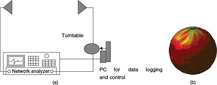
5.12.2.1.3 Measurements of Antenna Gain

Antenna gain measurements include absolute gain measurements with either two antennas or three antennas and the gain-transfer (gain-comparison) method using a calibrated antenna such as a horn antenna. Here we describe the absolute gain method, which utilizes two identical antennas such as those used in the array for transmission and one for a reception and a spectrum analyzer [54] as shown in Figure 5.64. The method is based on the Friis transmission formula, which when expressed in logarithmic form is given by:

5.112

where is the input power to the transmitting antenna and is the measured power from the receiving antenna under test, is the wavelength and R is the separation between the transmitting antenna and receiving antenna. For identical transmitting and receiving antennas, Equation (5.112) reduces to:

5.113

Figure 5.64 Spectrum analyzer set up for measuring antenna gain [52]. Source: Abdalla M., Feeney S.M., Salous, S., and Lewenz R., (2010), Design and calibration of circular uniform beam array for wideband channel characterisation. IET Microwave Antennas Propag., Vol. 4, Iss. 1, pp. 43–53 43, doi: 10.1049/iet-map.2008.0273. Reproduced with permission of IET.

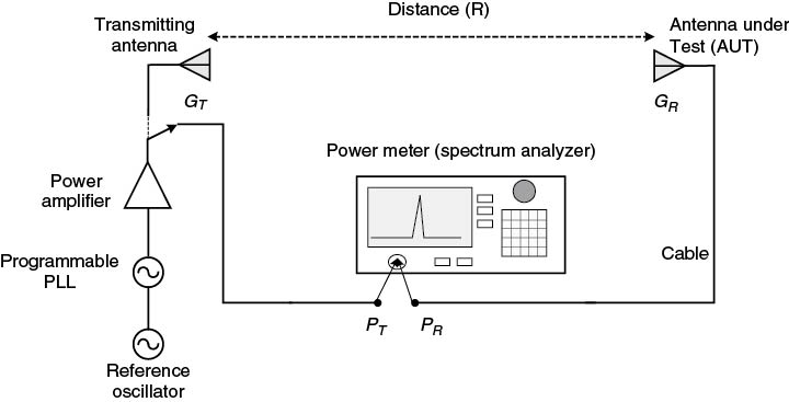
For known R (far-field distance), and the ratio of , the gain of the antenna can be computed.

5.12.2.1.4 Directivity and Radiation Efficiency

The antenna directivity D is evaluated from the half-power beamwidths (HPBWs) in the E and H planes; that is starting from the angle of maximum illumination the angles that are 3 dB less than the peak give the corresponding beamwidth. The assumption here that there is only one major lobe and all minor lobes, if present, have very low intensity.

The antenna radiation efficiency across the operating band is given by the ratio of the gain of the antenna G and its directivity D:

5.114

5.12.2.2 Calibration of the Overall Array Including Mutual Coupling

The effect of coupling between elements can be measured using two methods: (i) measuring the S_ij parameters where i≠j for all the elements of the array using a vector network analyzer and (ii) measurements of the radiation pattern in an anechoic environment with all antennas in the array present and active.

5.12.2.2.1 Measuring the S_ij Parameters Using a Network Analyzer

For stacked arrays, both the horizontal and vertical mutual coupling needs to be evaluated. An example of measuring the interelement cross coupling with frequency using a network analyzer is displayed in Figure 5.65a and b [55]. The mutual coupling is seen to decrease as a function of increasing the physical separation between the two antenna elements under test in both the horizontal and vertical directions. While increasing the separation reduces the coupling, it is necessary to choose the interelement separation to avoid spatial aliasing. In [53] it is proposed to add a component related to the complex values of the S parameters to the received signal to study the effect of mutual coupling on the estimated parameters including the time of arrival and DOA when using the SAGE algorithm.

Figure 5.65 Measured mutual coupling as a function of antenna element separation: (a) elements spaced horizontally and (b) elements spaced vertically [55].

Source: Abdalla, M. M., (2005) Directional antenna array for channel measurement system. PhD thesis University of Manchester Institute of Science and Technology. Reproduced with permission.

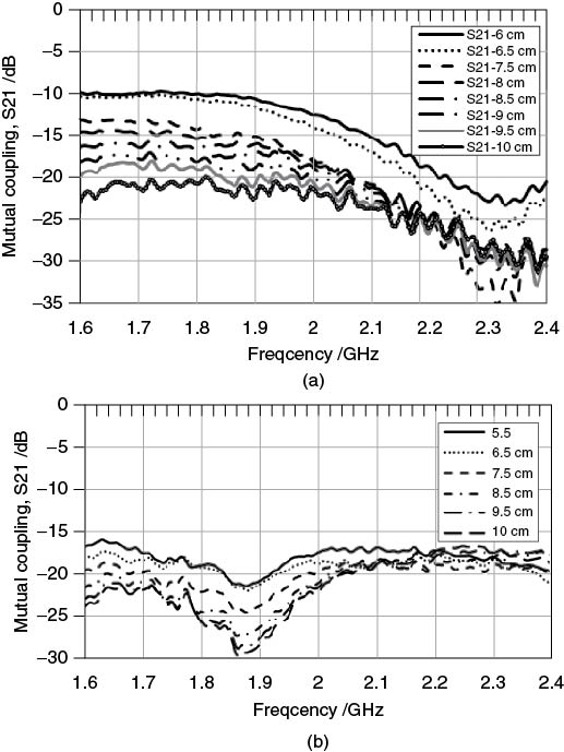
5.12.2.2.2 Measurements of Radiation Patterns

These measurements can also be performed using a vector network analyzer as in the case of the single element. Depending on the number of ports that are available for measurements, either each antenna element is measured in turn while all the other elements in the array are terminated or if a multiple port network analyzer is available several antennas can be measured simultaneously. Equally, an efficient and accurate alternative is to measure all the antenna elements simultaneously using a parallel custom-designed circuit, which can either measure the magnitude only of the radiation pattern or measure the complex function of each antenna element to provide magnitude and phase information [52]. Either method requires a turntable with a PC to control its motion in discrete angular steps, with the latter requiring a separate transmitter and a multichannel data acquisition card. An example of a custom-designed quadrature unit is displayed in Figure 5.66a with the single channel quadrature downconverter in Figure 5.66b. The unit consists of a reference channel and four identical quadrature measurement channels centred at 10 MHz with a bandwidth of ±1 MHz. Using suitable up- and downconverters to RF, the unit is independent of the frequency range under measurement. All oscillators are phase-locked to the 10 MHz reference signal thereby avoiding any phase drift effects. Each measurement channel provides the I' and Q' outputs that correspond to multiplying the input signal with the in-phase and quadrature components of the local signal from the reference channel-tracking oscillator. The outputs can then be digitized using an eight channel data acquisition card synchronized to the controller of the turntable.

Figure 5.66 Block diagram of (a) the four channel calibration unit and (b) a single channel [52].

Source: Abdalla M., Feeney S.M., Salous, S., and Lewenz R., (2010), Design and calibration of circular uniform beam array for wideband channel characterisation. IET Microwave Antennas Propag., Vol. 4, Iss. 1, pp. 43–53 43, doi: 10.1049/iet-map.2008.0273. Reproduced with permission of IET.

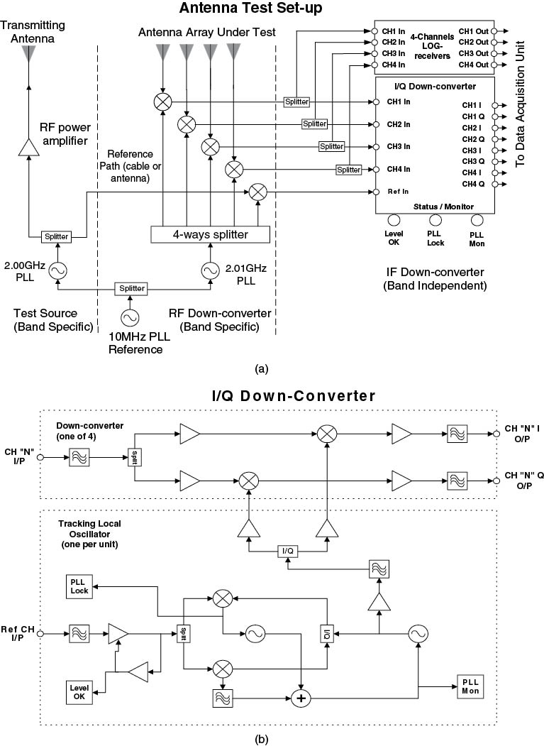
Figure 5.67 shows the amplitude and phase functions of two elements in the CUBA array displayed in Figure 5.61 and their corresponding phase response. The overall response of the array is displayed in Figure 5.68a,b where (a) is the polar plot of amplitude as a function of azimuth and (b) is the corresponding surface plot.

Figure 5.67 The amplitude and phase functions of two elements in the CUBA array displayed in Figure 5.61 and their corresponding phase response. The overall response of the array is displayed in Figure 5.68a,b where (a) is the polar plot of amplitude as a function of azimuth and (b) is the corresponding surface plot.

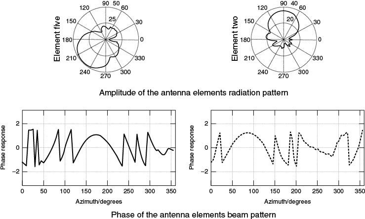
Figure 5.68 Measured radiation pattern of the CUBA array of Figure 5.61 [52]: (a) a polar plot and (b) a surface plot.

Source: Abdalla M., Feeney S.M., Salous, S., and Lewenz R., (2010), Design and calibration of circular uniform beam array for wideband channel characterisation. IET Microwave Antennas Propag., Vol. 4, Iss. 1, pp. 43–53 43, doi: 10.1049/iet-map.2008.0273. Reproduced with permission of IET.

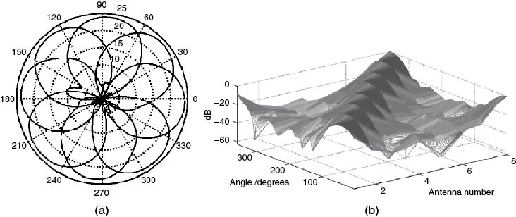
Figure 5.69 (a) Effective aperture distribution function (EADF) [52]. Source: Abdalla M., Feeney S.M., Salous, S., and Lewenz R., (2010), Design and calibration of circular uniform beam array for wideband channel characterisation. IET Microwave Antennas Propag., Vol. 4, Iss. 1, pp. 43–53 43, doi: 10.1049/iet-map.2008.0273. Reproduced with permission of IET. and (b) cross correlation function of the CUBA array of Figure 5.59 [59].

Source: Razavi-Ghods N., (2006), Characterisation of MIMO radio propagation channels. Thesis submitted to the degree of PhD, Durham University. Reproduced with permission.

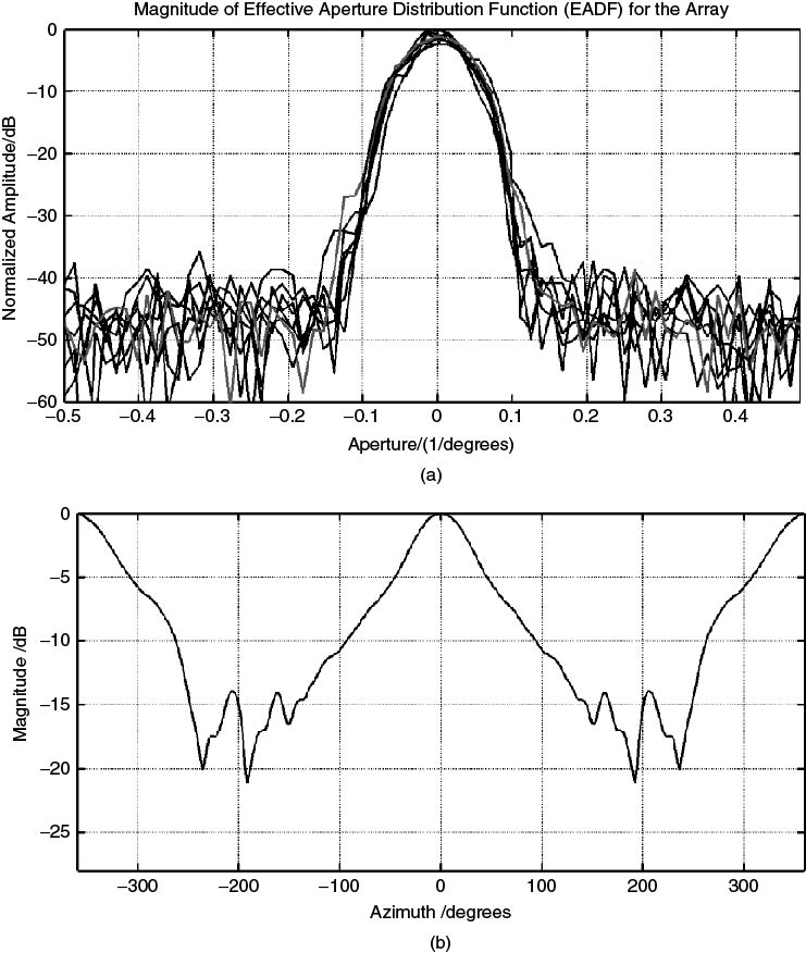
Two other functions describing the behaviour of antenna arrays when used with super-resolution algorithms such as SAGE are: (i) the effective aperture distribution function (EADF), which is obtained by applying the DFT to the complex beam pattern of the M antenna array, and (ii) the correlation function [51, 56]. Ideally the EADF should be evaluated with a 2D DFT from measurements of the array response in azimuth and in elevation and a sharp peak in the centre indicates good resolution properties in both angular directions as well as good calibration. Figure 5.69a and b displays the EADF and the correlation function of the eight-sector stacked array configuration using the measured complex beam pattern. The EADF shows the concentration of the function in a finite support area and hence a reduced amount of data can be stored to replicate the antenna beam pattern [51, 56]. The correlation function shows the cross correlation coefficient of the array response as a function of angle displacement. High cross correlation coefficients severely affect the resolution capability of the array for super-resolution algorithms, with the worst case scenario when the coefficients are as high as the main lobe. Figure 5.69b shows that the cross correlation at an angular distance of approximately 60° is roughly 5 dB below the main peak, which would be suitable for high resolution DOA estimation.

5.12.3 Estimation of Direction of Arrival

The first step in the estimation of the angle of arrival is the compensation for the gain settings from back-to-back calibration files of the sounder and for the antenna gain of each element in the array. This is particularly important when the data are acquired with a multiple receiver channel sounder. Following calibration the data can be processed using any of the array processing algorithms. Figure 5.70 displays the average impulse response in an LOS scenario using the CUBA array in Figure 5.61b obtained from measurements at 1.95 GHz with a 60 MHz bandwidth. Considering the main component in the dotted ellipse, we can see from the figure that antenna four has the strongest signal level.

Figure 5.70 Power delay profile as received on the eight element CUBA array of Figure 6.61 normalized with respect to the maximum of all elements.

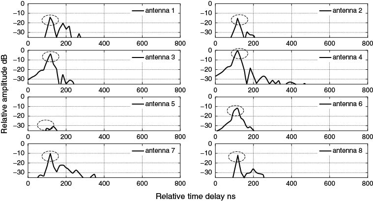
Applying the Capon beam forming algorithm to the impulse response and choosing the result for the DOA for the two strongest components in the delay profile we get Figure 5.71a, which gives the DOA as a function of the time delay (the time delay is indicated by rings extending up to 25 ns). Figure 5.71b displays the polar diagram of the fourth antenna element. The polar diagram shows the coincidence of the DOA with the corresponding antenna beam. Both multipath components are seen to arrive from the same direction but with a difference in time delay of ∼66 ns with corresponding angles of arrival estimated at 355° and 354°, respectively. The beam forming plot shows fairly broad lobes for each component, which indicates poor resolution in the presence of multiple components arriving from closeby angles.

Figure 5.71 Polar diagram identifying the multipath components in the time delay and angle of arrival using Capon beam forming and (b) polar diagram of the fourth antenna element.

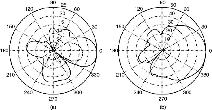
Using the same set of data and applying the SAGE algorithm initialized with the time delay of the two components, the DOA of the two components are estimated at 338° and 340°, respectively. For high bandwidth channel sounders, the search time in the SAGE algorithm can be reduced by initialization from the impulse response of the channel following the identification of the multipath components in the time delay.

Figure 5.72a displays an example of a dense multipath environment with echoes extending up to 5.8 µs. Estimating the DOA of the multipath components using the SAGE algorithm gives Figure 5.72b, which again displays the DOA as a function of time delay. Since the array consists of directional elements, the angular spread of the multipath components can also be inferred from the PDP. By normalizing the display in the time delay and angle of arrival with respect to the first arriving component, the farthest component and the first arriving component are seen to be strongest on the third antenna element. Upon application of the SAGE algorithm they are both identified with an angular direction of 150°.

Figure 5.72 (a) Power delay profiles obtained on the eight element CUBA array. (b) Polar diagram identifying the multipath components in the time delay and angle of arrival using the SAGE algorithm [52]. Source: Abdalla M., Feeney S.M., Salous, S., and Lewenz R., (2010), Design and calibration of circular uniform beam array for wideband channel characterisation. IET Microwave Antennas Propag., Vol. 4, Iss. 1, pp. 43–53 43, doi: 10.1049/iet-map.2008.0273. Reproduced with permission of IET.

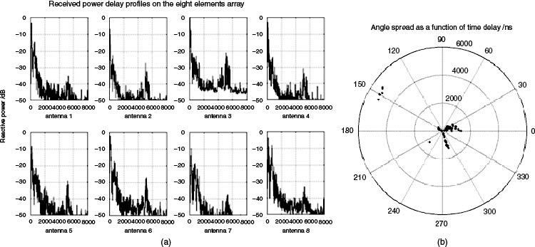
5.12.4 Estimation of Direction of the Arrival/Direction of Departure

When multiple antennas are employed at the transmitter and at the receiver the data can be processed to obtain the angle of arrival and angle of departure. In order to obtain the double-directional information it is necessary to calibrate the antenna arrays at both ends of the link to obtain the joint steering vector:

5.115

where a(θ_Tx) and a(θ_Rx) are the array steering vectors at the transmitter and at the receiver respectively and ⊗ represents the Kronecker product [58]. Using the Capon beamformer the modified expression for the estimation of the Capon spectrum is now given by:

5.116

where {·}^H is complex conjugate transpose, θ_Tx and θ_Rx are azimuth angles at the transmitter and at the receiver respectively and is the sample covariance matrix given by:

5.117

where K is the total number of frequency bins and h^(k) = Vec{H(k)} where the vector operation Vec {·} stacks a matrix into a vector [58].

Similarly, the data can be analyzed using the SAGE algorithm following the stacking of the data into a vector and adding another parameter corresponding to the angle of departure. Figure 5.73 gives an example of a double-directional estimation of an indoor radio channel obtained with two 6 × 8 CUBA arrays. The results can then be analyzed to identify multipath clusters, which represent groups of multipath components arriving/departing from similar angles and from similar time delays or can be analyzed to estimate the RMS angle spread.

Figure 5.73 Angle of departure/angle of arrival estimated from a 6 × 8 MIMO measurement in an indoor environment [60].

Source: Razavi-Ghods, N., and Salous S., (2009), Wideband MIMO channel characterization in TV studios and Radio Sci., 44, RS5015, doi:10.1029/2008RS004095. Reproduced in accordance with guidelines from Radio Science.

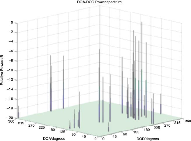
5.13 Estimation of MIMO Capacity

Estimation of n × m MIMO capacity is achieved from the time-variant frequency response for wideband signals by computing the narrowband channel capacity and taking the average over all the frequencies N_f in the band as in:

5.118

Thus, depending on the architecture of the sounder the impulse response of the channel is Fourier transformed to obtain the time-variant frequency response over a number of snapshots. Prior to taking the Fourier transform the dynamic range of the PDP is verified for a particular SNR, for example 20–30 dB. To reduce the effect of noise in the measured data it is also possible to select the start and the end of the impulse response, through filtering prior to taking the Fourier transform. The effect of phase noise of the local oscillator has been shown to increase the estimated channel capacity [60] and to affect the measurement of keyhole.

Other factors to consider in the processing of MIMO measurements is the normalization of the data to eliminate the effect of path loss as a function of location and the isolation between the antenna elements in particular when an RF switch is used at the transmitter and at the receiver. Poor isolation between the outputs of the switch increases the correlation between the elements and reduces the channel capacity. A consideration in the choice of the switch is its performance as a function of frequency for studies that require multiple frequency band measurements.

As discussed in Chapter 3, MIMO channel capacity is dependent on the correlation between the different antenna elements at both ends of the link. The correlation coefficients can also be computed using , which is the kth channel frequency bin in each frequency response from the jth transmit element to the ith receive element [61, 62]. For example, the correlation coefficient at the receiver with particular element spacing is defined as:

5.119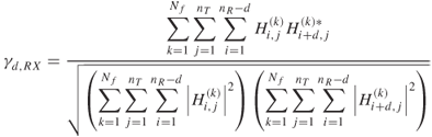

where d is the element spacing, typically defined as 1. The transmit correlation coefficient is calculated by interchanging the roles of the transmitter and receiver [61].

References

1. Harris, F.J. (1978) On the use of windows for harmonic analysis with the discrete Fourier transform. Proc. IEEE, 66 (1), 51. DOI: 10.1109/PROC.1978.10837 DOI:dx.doi.org.

2. Nuttall, A.H. (1981) Some windows with very good sidelobe behavior. IEEE Trans. Acoust. Speech Signal Proc., 29 (1), 84–91. DOI: 10.1109/TASSP.1981.1163506 DOI:dx.doi.org.

3. Salous, S. and Khadra, L. (1989) Measuring the coherence of wideband dispersive channels. J. Electron. Commun., 1 (5), 205–209.

4. Salous, S. (1997) On the potential applicability of auto-regressive spectral estimation to HF chirp sounders. J. Atmos. Solar Terr. Phys., 59 (15), 1961–1972.

5. Shearman, E.D.R. and Unsal, R.R. (1980) Compatibility of high-frequency radar remote sensing with communications. International Conference on Radio Spectrum Conservation Techniques, London, England, July 7–9, Proceedings. (A82-23801 09–32), Institution of Electrical Engineers, London, pp. 103–107.

6. Salous, S. (1986) An FMCW channel sounder with digital processing for measuring the coherence of wideband HF radio links. IEE Proc. F., 133 (5), 456–462.

7. Marple Jr, S.L. (1987) Digital Spectral Analysis with Applications, Prentice Hall.

8. Kay, S.M. and Marple Jr, S.L. (1981) Spectrum analysis – a modern perspective. Proc. IEEE, 69 (11), 1380–1419.

9. Salous, S. and Gokalp, H. (2007) Medium and large scale characterisation of UMTS allocated frequency division duplex channels. IEEE Trans. Veh. Technol., 56 (5), 2831–2843.

10. Gokalp, H., Taflan, G.Y. and Salous, S. (2009) In-band interference reduction in FMCW channel data using prony modelling. Electron. Lett., 45 (2), 132–133.

11. Sousa, E.S., Jovanovik, V.M. and Daigneault, C. (1994) Delay spread measurements for the digital cellular channel in Toronto. IEEE Trans. Veh. Technol., 43, 4, 837–847.

12. Schwartz, M., Bennett, W. R and Stein, S. (1966) Communication Systems and Techniques, McGraw-Hill, New York.

13. Salous, S. and Gokalp, H. (2002) Dual-frequency sounder for UMTS frequency-division duplex channels. IEE Proc. Commun., 149 (2), 117–122.

14. Cox, D. (1972) Delay Doppler characteristics of multipath propagation at 910 MHz in a suburban mobile radio environment. IEEE Trans. Antennas Propag., 20 (5), 625–635.

15. Bajwa, A.S. and Parsons, J.D. (1982) Small-area characterisation of UHF urban and suburban mobile radio propagation. IEE Proc., F Commun., Radar Signal Process., 129 (2), 102–109.

16. Turkmani, A.M.D., Demery, D.A. and Parsons, J.D. (1991) Measurement and modelling of wideband mobile radio channels at 900 MHz. IEE Proc. I Commun., Speech Vision, 138 (5) 447–457.

17. Turin, G.L., Clapp, F.D., Johnston, T.L. et al. (1972) A statistical model of urban multipath propagation. IEEE Trans., VT-21 (l), 1–9.

18. Bultitude, R.J.C., Mahmoud, S.A. and Sullivan, W.A. (1989) A comparison of indoor radio propagation characteristics at 910 MHz and 1.75 GHz. IEEE J. Sel. Areas Commun., 7 (1), 20–30.

19. Seidel, S.Y. Rappaport, T.S., Jain, S. et al. (1991) Path loss, scattering, and multipath delay statistics in four European cities for digital cellular and microcellular radiotelephone. IEEE Trans. Veh. Technol., 40 (4), 721–730.

20. Devasirvatham, D.J.M. (1986) Time delay spread and signal level measurements of 850 MHz radio waves in building environments. IEEE Trans. Antennas Propag., 34 (11), 1300–1305.

21. Bendat J.S. and Peirsol, A.G. (1966) Measurements and Analysis of Random Data, John Wiley & Sons, Inc., Hoboken, NJ, p. 170.

22. Bultitude, R.J.C. (2002) Estimating frequency correlation functions from propagation measurements on fading radio channels: a critical review. IEEE J. Sel. Areas Commun., 20 (6), 1133–1143.

23. Bultitude, R.J.C. (1983) A study of coherence bandwidth measurements for frequency selective radio channels. Proceedings of the 33rd IEEE VTC, pp. 269–277.

24. Feuerstein, M.J., Blackard, K.L., Rappaport, T.S. et al. (1994) Path loss, delay spread and outage models as functions of antenna height for microcellular system design. IEEE Trans. Veh. Technol., 43 (3), 487−497.

25. Greenstein, L.J., Erceg, V., Yeh, Y.S. and Clark, M.V. (1997) A new path-gain/delay-spread propagation model for digital cellular channels. IEEE Trans. Veh. Technol., 46 (2), 477−485.

26. Krim, H. and Viberg, M. (1996) Two decades of array signal processing research: the parametric approach. IEEE Signal Process. Mag., 13 (4), 67–94 (Special Issue on Array Processing).

27. Burg, J.P. (1967) Maximum entropy spectral analysis. Proceedings of the 37th Annual International SEG Meeting, Oklahoma City.

28. Capon, J. (1969) High resolution frequency wave number spectrum analysis. Proc. IEEE, 57, 1408–1418.

29. Pisarenko, V.F. (1973) The retrieval of harmonics from a covariance function. Geophys. J. Roy. Astron. Soc., 33, 347–366.

30. Bienvenu, G. and Kopp, L. (1980) Adaptivity to background noise spatial coherence for high resolution passive methods. Proceedings of the IEEE ICASSP, Denver, CO, pp. 307–310.

31. Schmidt, R.O. (1981) A signal subspace approach to multiple emitter location and spectral estimation. PhD Dissertation, Stanford University, Stanford, CA.

32. Roy, R.H. (1987) ESPRIT, estimation of signal parameters via rotational invariance techniques. PhD Dissertation, Stanford University, Stanford, CA.

33. Roy, R. and Kailath, T. (1989) ESPRIT – estimation of signal parameters via rotational invariance techniques. IEEE Trans. Acoust. Speech Signal Process., 37 (7), 984–995.

34. Haardt, M. and Nossek, J. (1995) Unitary ESPRIT: how to obtain increased estimation accuracy with a reduced computational burden. IEEE Trans. Signal Process., 43 (5), 1232–1242.

35. Fessler, J.A. and Hero, A.O. (1994) Space-alternating generalized expectation maximization algorithm. IEEE Trans. Signal Process., 42, 2664–2677.

36. Fleury, B.H., Tschudin, M., Heddergott, R. et al. (1999) Channel parameter estimation in mobile radio environments using the SAGE algorithm. IEEE J. Sel. Areas Commun., 17 (3), 434–449.

37. Fleury, B.H., Dahlhaus, D., Heddergott, R. and Tschudin, M. (1996) Wideband angle of arrival estimation using the SAGE algorithm. Proceedings of the IEEE ISSSTA, Mainz, Vol. 1, pp. 79–85.

38. Dacos, I. and Manikas, A. (1995) Estimating the manifold parameters of one dimensional arrays of sensors. J. Franklin Inst. Eng. Appl. Math., 332B (3), 307–332.

39. Godara, L.C. (2002) Handbook of Antennas in Wireless Communications, CRC Press.

40. Chan, T.F. (1987) Rank-revealing QR factorisation. Linear Algebra Appl., 89, 67–82.

41. Stewart, G.W. (1992) An updating algorithm for subspace tracking. IEEE Trans. Signal Process., 40, 1535–1541.

42. Van der Veen, A.J. and Godge, J. (1994) On-line subspace estimation using a generalized schur method. Proceedings of the 7th IEEE SP Workshop on Statistical Signal and Array Processing, Quebec City, Canada, pp. 87–90.

43. Barabell, A.J. (1983) Improving the resolution performance of eigenstructure based direction-finding algorithms. Proceedings of the ICASSP 83, Boston, MA, pp. 336–339.

44. Gleser, L.J. (1981) Estimation in a multivariate 'errors in variables' regression model: large sample results. Ann. Stat., 9, 22–44.

45. Roy, R., Ottersten, B., Swindlehurst, L. and Kailath, T. (1992) Multiple invariance ESPRIT. IEEE Trans. Acoust., Speech Signal Process., 40 (4), 867–881.

46. Erhel, Y., Lemur, D., Bertel, L. and Marie, F. (2004) HF radio-direction finding operating on a heterogeneous array: principles and experimental validation. Radio Sci., 39, RS1003. DOI: 10.1029/2002RS002860

47. Manikas, A., Alexiou, A. and Karimi, H.R. (1997) Comparison of the ultimate direction-finding capabilities of a number of planar array geometries. IEE Proc. Radar Sonar Navig., 144 (6), 321–329.

48. Marie, F., Erhel, Y., Bertel, L. and Lemur, D. (2000) Design of a HF compact direction finding system based on colocated antennas. Proceedings of the 8th International Conference on HF Radio Systems and Techniques, IEE Conference Publication, 474, 127–131.

49. Oger, M., Marie, F., Lemur, D. et al. (2006) A method to calibrate HF receiving antenna arrays. 10th International Conference on Ionospheric Radio Systems and Techniques (IRST 2006), Institute of Engineering and Technology, London.

50. Gunashekar, S.D., Warrington, E.M., Strangeways, H.J. et al. (2009) Utilization of antenna arrays in HF systems. Ann. Geophys., 52 (3/4), 323–338.

51. Tan, C.M., Landmann, M., Richter, A. et al. (2002) On the application of circular arrays in direction finding part ii: experimental evaluation on SAGE with different circular arrays. 1st Annual COST 273 Workshop, Espoo, Finland.

52. Abdalla, M., Feeney, S.M., Salous, S. and Lewenz, R. (2010) Design and calibration of circular uniform beam array for wideband channel characterisation. IET Microwave Antennas Propag., 4 (1), 43–53. DOI: 10.1049/iet-map.2008.0273.

53. Verhaevert, J., Van Lil, E. and De Capelle, A.V. (2002) Influence of coupling in antenna arrays on the SAGE algorithm. Proceedings of the URSI GA02, Paper 0508.

54. Balanis, C.A. (1997) Antenna Theory: Analysis and Design, 2nd edn, John Wiley & Sons, Inc., New York.

55. Abdalla, M.M. (2005) Directional antenna array for channel measurement system. Thesis submitted to the degree of PhD, Manchester University.

56. Landmann, M., Thoma, R.S. and Richter, A. (2003) Performance evaluation of real antenna arrays for high-resolution DoA estimation in channel sounding – Part 1: channel parameter resolution limits. COST 273 Temporary Document, TD(03)199, Prague, Czech Republic.

57. Almers, P., Wyne, S., Tufvesson, F. and Molisch, A. (2005) Effect of Random Walk Phase Noise on MIMO Measurements, Mitsubishi Electric Research Laboratories, http://www.merl.com.

58. Eugene, C.H.Y., Sakaguchi, K. and Araki, K. (2004) Experimental and analytical investigation of MIMO channel capacity in an indoor line-of-sight (LOS) environment. 15th IEEE International Symposium on Personal, Indoor, and Mobile Radio Communications (PIMRC 2004), Barcelona, Spain.

59. Razavi-Ghods, N. (2006) Characterisation of MIMO radio propagation channels. Thesis submitted to the degree of PhD, Durham University.

60. Razavi-Ghods, N. and Salous, S. (2009) Wideband MIMO channel characterisation in TV studios and inside buildings in the 2.2–2.5 GHz frequency band. Radio Sci., 44, RS5015. DOI: 10.1029/2008RS004095.

61. Maharaj, B., Wallace, J. and Jensen, M. (2005) Comparison of double-directional channel response at 2.4 and 5.2 GHz from indoor co-located wideband MIMO channel measurements. XXVIIIth URSI GA, New Delhi, India.

62. Maharaj, B.T., Wallace, W., Linde, L.P. and Jensen, M.A. (2005) Frequency scaling of spatial correlation from co-located 2.4 and 5.2 GHz wideband indoor MIMO channel measurements. IEE Electron. Lett., 41, 336–337.