Appendix 1

A.1 Probability Distribution Functions

In this appendix we give the probability density functions (PDFs) and the basic properties of the most commonly used statistical distributions in the characterization of the fading envelope of the received signal. These include the Rayleigh, the Rician, the Nakagami m-distribution, Weibull, the log-normal, the Suzuki and the chi-square distributions. In addition, we give the Gaussian distribution used to represent thermal noise, which is also used in the generation of Rayleigh distribution.

A.2 The Gaussian (Normal) Distribution

A random variable r is said to be normally distributed with mean μ and variance σ² if its probability density function is:

A.1

Since the normal or Gaussian distribution is fully characterized by its mean and variance or standard deviation σ it is usually represented by:

A.2

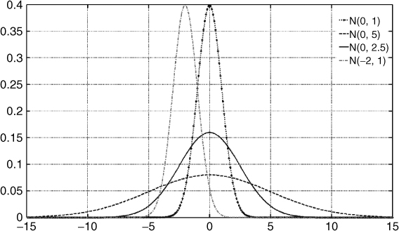
The Gaussian distribution has a bell-shaped curve with its maximum value of occurring at the mean value μ. Figure A.1 illustrates the distribution for different values of the mean and standard deviation σ where it can be seen that the standard deviation is related to the dispersion around the mean.

The mean and variance of the normal distribution are given by:

A.3

A.4

The cumulative distribution of the Gaussian PDF is given by:

A.5

Figure A.2 displays the cumulative distribution function (CDF) of the Gaussian distributions in Figure A.1. The figure shows the effect of the standard deviation on the CDF where the smaller standard deviation gives rise to a steeper curve. The effect of the mean is seen to shift the overall CDF curve where the median value of 0.5 occurs at the mean value.

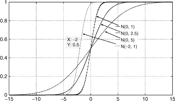
The Gaussian distribution satisfies the 68, 95, 99.7 rule, which is also known as the three-sigma rule or empirical rule, which states that for a normal distribution 68 % of the values are within a standard deviation, 95 % of the values are within two standard deviations and 99.7 % of the values are within three standard deviations of the mean.

A.3 The Rayleigh Distribution

The Rayleigh distribution arises when two independent Gaussian distributed processes I(t) and Q(t) with zero mean and equal variance are combined to generate the envelope . Thus, in addition to the fading envelope of the received signal in the presence of a large number of multipath components with equal amplitude and uniform phase distribution, the Rayleigh distribution also represents the envelope of white Gaussian noise where the in-phase and quadrature components have zero mean with equal variance.

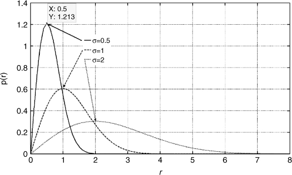
The Rayleigh PDF of a random variable r is given by Equation (A.6) (see also Equation (5.22) in Chapter 5):

A.6

where is the mode of the distribution and represents the value that occurs most frequently in the PDF, as illustrated in Figure A.3 for different values of .

The mean value of the distribution is given as:

A.7

and the mean square value is found from:

A.8

The variance is then given by:

A.9

This gives a standard deviation of r, equal to .

The Rayleigh CDF, which gives the probability of r being less than R, P_r (R), is given by:

A.10

The median value can be found by setting R = and P_r () = 0.5, as given by:

A.11

Other expressions for the PDF and CDF can be written in terms of the mean square value, the mean and the median [1].

In terms of the mean square value, we obtain:

A.12

In terms of the mean :

A.13

In terms of the median,

A.14

A.4 The Rician Distribution

The Rician PDF was first proposed by Rice [2] in 1945 while studying the distribution of noise current. Rice showed that given a sinusoid with amplitude s in additive noise, as in:

A.15

where n(t) is the noise component consisting of the sum of N sinusoids each with frequency and phase for n = 1, … N, which are independent random variables [2]. The distribution of the envelope r(t) is given by the Rician PDF as in:

A.16

where I_o(.) is the modified Bessel function of the first kind and zero order, and σ is the standard deviation of the independent Gaussian processes representing the in-phase and quadrature components of noise. Equivalently, the Rice distribution arises when two independent Gaussian distributed processes I(t) and Q(t) with nonzero mean and each with a variance equal to σ are combined to generate .

In a multipath environment the Rician distribution arises when the received signal has a large number of multipath components each with its own Doppler shift and phase in addition to a deterministic component that could be the line of sight component or the line of sight, plus a ground reflection with its own Doppler shift and initial phase. By the central limit theorem the in-phase and quadrature components I(t) and Q(t) of the received signal at one particular instant t_o I(t_o) and Q(t_o) are Gaussian, but, due to the deterministic dominant term, no longer have zero mean. If s is zero, the distribution becomes Rayleigh and the in-phase and quadrature components have zero mean.

The Rician distribution is often described by the K factor, which is defined as the ratio of power in the dominant component over the local mean power of the multipath components. In a linear scale the K factor is given by:

A.17

Given a set of measurements the K factor can be estimated using the method of moments where:

A.18

where m₂ and m₄ are the second and fourth order moments as estimated from the data, where:

A.19

A.5 The Nakagami m-Distribution

The Nakagami distribution was first proposed to fit measurements over ionospheric links [3]. Unlike the Rayleigh model where the amplitude of the multipath components are assumed to be equal, the Nakagami distribution permits the amplitude variations to be random and not necessarily of almost equal level.

The Nakagami m-PDF of r is given by:

A.20

where the parameter m is called the ‘shape factor’ of the Nakagami or the gamma distribution and Γ (.) is the gamma function, the mean square and:

For m = 1, the Nakagami distribution reduces to Rayleigh fading with an exponentially distributed instantaneous power and for m = 1/2, it reduces to the one-sided Gaussian distribution. When m is near but greater than unity, the Rice distribution is approximated by:

A.21

Although this approximation may be accurate for the main body of the probability density, it can become highly inaccurate for the tails. Since bit errors or outages mainly occur during deep fades, which are represented by the tail of the probability density function, it is inaccurate to approximate the fading of the wanted Rician signal by a Nakagami model for the performance prediction of systems.

The Nakagami distribution also approximates the log-normal distribution for large m on the domain:

A.22

In addition to modelling empirical data the Nakagami distribution describes well the sum of multiple independent and identically distributed (IID) Rayleigh fading signals. Thus it can be useful in describing the resulting signal from a maximum ratio combining diversity system, interference from multiple sources in a cellular system and for multipath scattering with a relatively large time delay spread with different clusters of reflected waves with significant difference in time delays.

A.6 The Weibull Distribution

The Weibull PDF is widely used to represent sea scatter. For a variable r, the Weibull PDF is given by:

A.23

where α is the shape parameter and β is the scale parameter. With β^α = 2σ², the Weibull distribution becomes a Rayleigh distribution when α = 2. For α = 1 it reduces to the exponential distribution.

A.7 The Log-Normal Distribution

The log-normal PDF is given by:

A.24

where m and σ are the mean and the standard deviation of ln(r). Using the method of maximum likelihood estimators the mean value and the variance are given by:

A.25

This distribution is used to explain large-scale variations (shadowing) of the signal strength in a multipath fading environment and for interference modelling in cellular networks.

A.8 The Suzuki Distribution

This is a combination of Rayleigh and log-normal distributions. Suzuki developed the PDF of the envelope in dB terms, which is given by:

A.26

where

m = is the mean of the Rayleigh distribution (dB)

σ_dB = is the deviation of the mean value (dB) and

= is normally distributed.

The Suzuki distribution describes when one or more relatively strong signals arrive at the receiver. The Suzuki distribution is rather complicated for data reduction because of the integral in the PDF.

A.9 The Chi-Square Distribution

The chi-square distribution is closely related to the Rayleigh distribution where r is replaced by r². In general if,

A.27

and are Gaussian distributed with zero mean, z will be chi-square distributed with n degrees of freedom. If all the Gaussian variables have a standard deviation of 1, the form of the density function is given by:

A.28

where ! indicates the factorial operation.

References

1. Parsons, J.D. (2000) The Mobile Radio Propagation Channel, John Wiley & Sons, Inc.

2. Rice, S.O. (1945) Mathematical analysis of random noise. Bell Syst. Tech. J., 2 (1), 46–156.

3. Nakagami, M. (1960) The m-distribution – a general formula of intensity distribution of rapid fading, in Statistical Methods of Radio Wave Propagation (ed. W.C. Hoffman), Pergamon Press.