Chapter 6
Radio Link Performance Prediction
Link channel performance can be estimated either from: (i) analytical predictions based on theoretical models or (ii) software simulators or hardware emulators using stochastic or deterministic channel models. Another possibility is to generate the channel parameters or to test the performance of the radio system from measurements in typical environments or in a reverberation chamber that is capable of emulating a multipath environment.
Channel models can be realized either in the time domain or in the frequency domain. A deterministic channel model has constant model parameters whereas a stochastic channel model has some or all of the model parameters being characterized by a stochastic distribution that is either ergodic or nonergodic [1]. An ergodic channel model requires only a single sample function or a single trial to characterize its stochastic properties whereas a nonergodic model requires several realizations where the average over a large number of trials is used to represent the performance of the channel. Further, channel models can be classified as narrowband versus wideband where the wideband channel can be considered as the sum of several narrowband channels with different delays.
In this chapter we start by studying narrowband and wideband channel simulators both in the time domain and in the frequency domain. We explain briefly software and hardware realization methods using analogue and digital techniques. This is followed by presenting a theoretical bit error rate (BER) performance for basic digital modulation schemes in the presence of additive white Gaussian noise (AWGN) for both optimum and suboptimum receivers. We then discuss the effect of channel impairments by investigating BERs using stochastic simulators and compare their performance against simulators using measured channel data. Prediction of the performance of three standards, two of which use orthogonal frequency division multiplexing (IEEE 802.16-d standard and the IEEE 802.11 standard) and the third, wideband code division multiple access (WCDMA), is presented from simulations using Matlab built-in SIMULINK channel simulators. Finally, we discuss the performance of multiple antenna systems using diversity gains to enhance the quality of service.
6.1 Radio Link Simulators
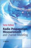
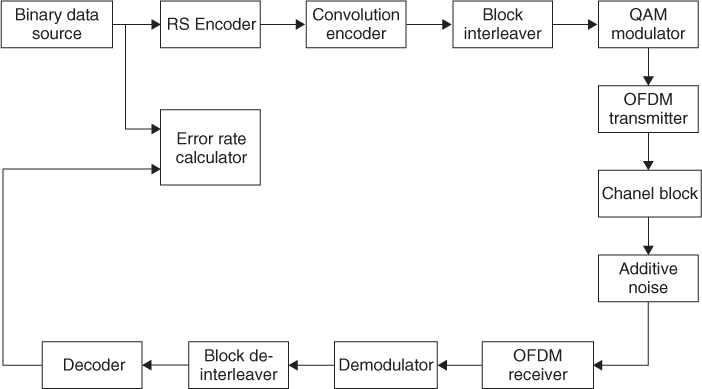
In digital communication the performance of a modulation scheme or a proposed standard is usually predicted from estimating BERs in the presence of AWGN and channel impairments as illustrated in the block diagram of Figure 6.1, where:
Figure 6.1 Block diagram of a communication system model including radio channel impairment block and additive noise.
In the absence of channel impairments the system's performance is usually evaluated in the presence of AWGN and the channel block is removed from the link between the transmitter and the receiver. When the channel is not ideal, then it is necessary to set up the appropriate channel block, which can be narrowband or wideband depending on the modulation scheme, the data rate and the channel fading characteristics. In Sections 6.2 and 6.3 we discuss the commonly used stochastic narrowband and wideband channel blocks for the evaluation of radio system performance and in Section 6.4 we present the frequency domain implementation of fast convolution followed by Section 6.5, where we present a channel block based on measurements in real environments. In Section 6.6 we study the effect of noise alone on the BER for the ideal matched filter and correlation detector and subsequently we discuss the effects of channel impairments on three wireless standards.
6.2 Narrowband Stochastic Radio Channel Simulator
A narrowband channel simulator assumes that all the frequency components in a signal undergo the same distortion as they travel through the channel. In a multipath environment this assumes that the multipath components are not resolved and a single channel coefficient that has the desired stochastic properties is sufficient. Narrowband fading simulators tend to assume that the channel coefficient either follows a Rayleigh distribution or a Rician distribution.
Over the years a number of simulators have been designed to generate the required complex channel coefficient. These include the uniform phase modulation method and the quadrature amplitude modulation (QAM) method. The power spectrum of the output signal of the uniform phase method cannot be easily controlled and hence tends not to be used in radio channel simulators and so will not be discussed here. In the following the quadrature amplitude domain method is outlined.
6.2.1 Quadrature Amplitude Modulation Simulator
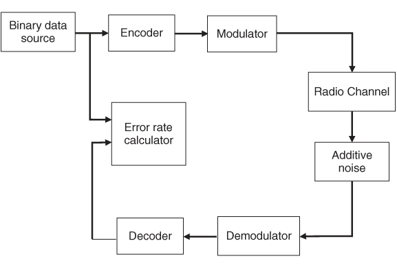
The basis for the quadrature simulator is the scattering model discussed in Chapter 3 where the received signal can be expressed in terms of the inphase (I(t)) and quadrature (Q(t)) components as given in:
For a Rayleigh distribution, the I and Q components are Gaussian distributed with zero mean and a variance equal to σ2 as illustrated in the block diagram of Figure 6.2. The Gaussian processes in Figure 6.2 are generated using one of two time domain methods or a frequency domain based method. The time domain methods are the filtered noise method and the sum of sinusoids. Measurements in reverberation chambers can also be used to generate the Rayleigh fading and these are also presented in this section.
Figure 6.2 Block diagram of a quadrature modulator.
6.2.2 Filtered Noise Method
The filtered noise method is based on using two white Gaussian noise (WGN) generators with zero mean and equal variances, which are subsequently filtered to have the desired Doppler spectrum with the required maximum Doppler frequency as illustrated in Figure 6.3 for the U-shaped spectrum. The filter's frequency response is the square root of the desired spectrum shape and can be implemented using either analogue or digital techniques where the digital implementation provides more flexibility as it enables modification of the maximum Doppler frequency without realizing a filter for each cut-off frequency. Figure 6.4 shows the fading waveforms for the inphase and quadrature components and the resultant Rayleigh fading signal for 40 Hz maximum Doppler shift.
Figure 6.3 Block diagram of a filtered noise simulator.
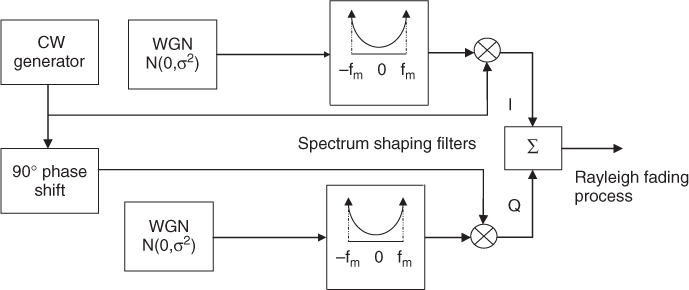
Figure 6.4 Waveforms generated in the simulator assuming a 40 Hz maximum Doppler shift: (a) in-phase component, (b) quadrature component and (c) resultant Rayleigh fading signal.

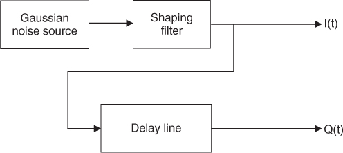
Central to the design of such a simulator is the noise generator, which can be implemented in the analogue domain via a simple noisy Zener diode [2] or in the digital domain with an m-stage maximal length feedback shift register, where the length is chosen to have the desired statistical properties [3]. In order to generate a white spectrum over the desired region of interest, the shift register is clocked at a rate much higher than the Nyquist rate of the final noise waveform. For example, in the implementation reported in [4] the register is clocked at 8 kHz to cover an 81 Hz cut-off frequency for the lowpass Doppler spectrum. In order to produce two uncorrelated Gaussian processes from one filter and one noise source the output of the shaping filter can be delayed as illustrated in Figure 6.5 [5]. A corresponding digital implementation of the generator can be realized using a shift register to generate the random noise sequence, a digital shaping filter and digital random access memories to implement the delay [4]. Using different clock rates to the different blocks generates different Doppler shifts to accommodate different vehicle speeds [4].
Figure 6.5 Block diagram of uncorrelated Gaussian generators using a delay line.
6.2.3 Sum of Sinusoids Method (Jakes Method)
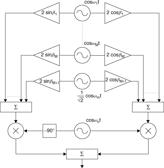
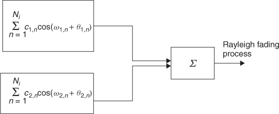
The basis of the sum of sinusoids (SOS) method is the generation of the in-phase and quadrature components represented in Equation (6.2), which consist of the sum of N sinusoids each with its amplitude, Doppler shift and phase shift. Depending on whether these three parameters are random variables or deterministic three possible SOS models can be realized: (i) the deterministic model, (ii) the ergodic stochastic model and (iii) the nonergodic stochastic model [1]. For the deterministic model, all three parameters are fixed whereas for the ergodic stochastic model the phase is a random variable and the amplitude and frequency are fixed. For the nonergodic model all three parameters are represented by random variables. Figure 6.6 displays the SOS simulator as proposed by Jakes [6] where the phase function ![]() is set to zero and M + 1 sinusoids are used to generate the quadrature components as given by:
is set to zero and M + 1 sinusoids are used to generate the quadrature components as given by:
6.3a ![]()
Figure 6.6 Block diagram of the sum of sinusoid simulator as proposed by Jakes [6, p. 70].
Source: Jakes W.C., (1994), Microwave Mobile Communications, New York: IEEE Press and John Wiley & Sons, Inc. Reproduced with permission.
and
6.3b ![]()
6.3c ![]()
and
6.3d ![]()
To produce a number of independent processes, Jakes suggested that the nth oscillator in the jth process has an additional phase shift ![]() , for example using the following relationships:
, for example using the following relationships:
6.4 ![]()
The SOS proposed by Jakes is simple and popular as it replicates the ideal U-shaped spectrum. However, it has two main shortcomings: (i) high cross correlation, in excess of 0.5 between generated processes when employed to simulate the frequency selective channel, and (ii) when the maximum Doppler shift frequency increases, the limited number of discrete frequency components can no longer approximate the specified spectrum [7, 8]. To overcome these limitations, Pätzold [9] proposed that the number of harmonics should be in excess of nine and Cavers [10] suggested using disjoint sets for the angles of arrival for different frequency generators.
Although analogue implementations are possible, digital implementation of the quadrature components provides flexibility in the number of sinusoids, programmable maximum Doppler frequency and compactness of the realization. The two baseband components can then be converted to analogue, filtered and mixed with the carrier in a quadratue modulator. Such implementations have been reported for a narrowband very high frequency/ultra-high frequency (VHF/UHF) simulator with Doppler rates from 2 to 126 Hz, in steps of 2 Hz [11], and in [12] modifications in the phase angles to generate multiple uncorrelated fading processes were incorporated with the jth pair of Gaussian noise processes given by:
6.5 
For eight sinusoids, the I(t) and Q(t) components approximate Gaussian processes and the correlation coefficients between the individual Gaussian processes could be adjusted between 0 and 1—a useful feature for the study of diversity techniques and MIMO systems.
A simple digital implementation can also be realized using lookup tables for the sinusoids, which only require a cyclic address generator and an adder to produce the Gaussian processes [13]. Another method used for the generation of Gaussian noise processes is Rice's sum of sinusoids [14, 15], which states that a Gaussian noise process μi(t). can be modelled by the superposition of an infinite number of weighted harmonic functions with equidistant frequencies and random phases according to [13, 16, 17]:
with the gains ![]() , where
, where ![]() is the Doppler power spectral density and discrete Doppler frequencies
is the Doppler power spectral density and discrete Doppler frequencies ![]() ,
, ![]() ,
, ![]() is uniformly distributed over the interval
is uniformly distributed over the interval ![]() .
.
The Gaussian process modelled by Equation (6.6) cannot be digitally implemented due to the infinite number of sinusoids. For a finite value of Ni the resulting process will not be Gaussian in the strict sense; however, for Ni ![]() 7, the PDF approaches a Gaussian process. Taking the sum [13] can be implemented as in Figure 6.7 and digital realization can be achieved by sampling the continuous Gaussian process in Equation (6.6) at t = kTs (k = 0, 1, 2,…), where Ts denotes the sampling interval.
7, the PDF approaches a Gaussian process. Taking the sum [13] can be implemented as in Figure 6.7 and digital realization can be achieved by sampling the continuous Gaussian process in Equation (6.6) at t = kTs (k = 0, 1, 2,…), where Ts denotes the sampling interval.
Figure 6.7 Block diagram representation of Equation (6.6) for generation of the sum of sinusoids based on the Rice model.
6.2.4 Frequency Domain Method
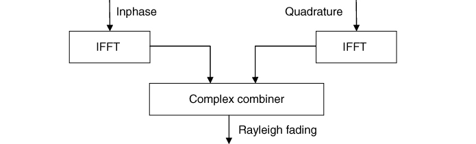
The frequency domain method proposed by Smith [18] generates N discrete samples from independent complex Gaussian random number generators along the positive frequency axis of the Doppler spectrum (0, fmax). The double-sided spectrum (−fmax, fmax) is then generated by taking the complex conjugate values as shown in Figure 6.8 [19], which are then multiplied by the square root of the 2N discrete realization of the U-shaped Doppler spectrum. The real value time domain Gaussian process is then generated via the inverse Fast Fourier transform IFFT [20]. The frequency separation between samples defines the time duration of a fading waveform. Two such generators are required for the quadrature components. To eliminate the need for two IFFT operations for the two components, Young and Beaulieu [20] proposed combining the two processes in the frequency domain and then performing a single IFFT. They have also shown that this method is the most efficient method in comparison with the SOS or the filtering method for the generation of correlated Rayleigh fading.
6.2.5 Reverberation Chambers (or Mode-Stirred Chambers)
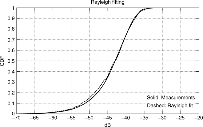
Reverberation chambers are electrically large chambers with approximately three or more wavelengths with highly reflecting walls and one or more rotating mode-stirrers, usually asymmetric in shape as illustrated in Figure 6.9a. Such chambers emulate a Rayleigh fading multipath environment by generating a large number of reflections. The measurements are usually performed using a multiple-port network analyzer placed outside the chamber and measuring the various S parameters such as S12 for the configuration of Figure 6.9b. To obtain the Rayleigh fading statistics several measurements at a sufficiently large number of positions, usually on the order of 200 positions, need to be performed at different stirrer positions [21]. This is equivalent to keeping the stirrer still and placing the antennas in different locations in the chamber. Figure 6.10 shows an example of a measured cumulative distribution function (CDF) with the corresponding fit (dashed line in the figure) verified using the Kolomogrov–Smirnoff test of the fading statistics to the Rayleigh distribution. In channel simulators, the data can be used instead of the Rayleigh generators in a ‘playback’ mode.
Figure 6.9 (a) Stirrer in reverberation chamber and (b) measurement set-up in the reverberation chamber.
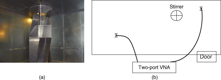
Figure 6.10 Cumulative distribution function of measurement in the reverberation chamber (solid line) and the Rayleigh fit to the data (dashed line).
The reverberation chamber can also be used to generate Rayleigh fading statistics for multiple antenna configurations including multiple input–single output (MISO), single input–multiple output (SIMO) and MIMO channels to assess both diversity gains and MIMO capacity. In this case more antennas are set up at the transmitter or receiver or both, depending on the application, and a multiple-port network analyzer is used, depending on the number of antennas.
6.3 Wideband Stochastic Channel Simulator
Wideband channel simulators are based on the wideband channel models discussed in Chapter 3. These are classified as (i) time domain models using the tapped delay line or transversal filter to represent the time-variant impulse response or (ii) frequency domain models based on the time-variant frequency response, which uses a number of filters with time-varying coefficients. These two models are interrelated with a Fourier transform relationship and the majority of reported implementations both in hardware and in software have been for the tapped delay line. In this section we discuss the realization of both types of simulators.
6.3.1 Time Domain Channel Simulators
The time domain simulator implements the time-variant impulse response of the channel as a time-variant linear finite impulse response (FIR) filter with the output of the channel being the convolution of the input with the impulse response as illustrated in Figure 6.11 and given by:
6.7 
Figure 6.11 Time domain wideband channel model.
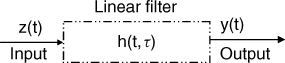
Since the impulse response extends over a time interval as determined by the extent of multipath components, the time axis can be subdivided into a number of subintervals where each subinterval has a number of unresolved multipath components and represents one Rayleigh fading path. The time delays are expressed with respect to the first significant path and can be related to the bandwidth of measurements or the bandwidth of the communication system to be analyzed. Not all time delays are used, depending on the multipath structure. This is equivalent to considering the wideband channel as many narrowband channels at different time delays. Hence, the wideband implementation consists of a delay line and Rayleigh fading generators as illustrated in the tapped delay line model in Figure 6.12. The Rayleigh generators can be implemented using any of the generators previously outlined where it is necessary to ensure that they are statistically independent. Using two Gaussian generators for each Rayleigh process, in-phase and quadrature modulation can be implemented as in Figure 6.2. In wideband channel simulations the power of each path is relative and the total power of the channel is usually normalized to unity to preserve the power of the input signal [10]. Therefore, the sum of variances of all the random processes in the tapped delay line model should be unity. This unit variance is distributed among each tap, depending upon the simulated power delay profile.
Figure 6.12 Tapped delay line wideband channel model.
The delay lines can be realized either in the analogue domain using surface acoustic wave (SAW) devices or digitally using, for example, first in–first out (FIFO) devices. The application of SAW devices permits the realization of long relative delays on the order of 10 µs due to the low propagation velocity of acoustic waves on the surface of the substrate.
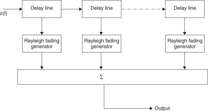
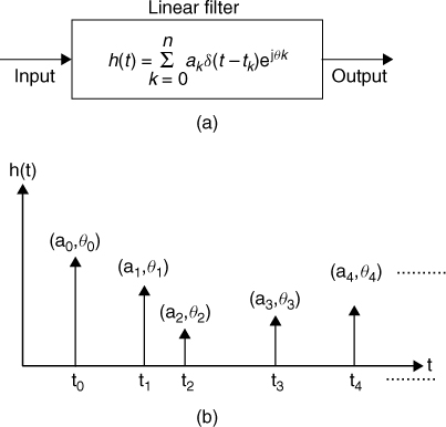
Digital implementations of the time-variant impulse response are based on a discrete channel model expressed as the sum of weighted impulses as shown in Figure 6.13 where the coefficients ![]() are random variables representing the amplitude, arrival time and phase angle of the kth path respectively. This model was proposed by Turin et al. [22] and its software realization was first reported in [23], which employed experimental propagation parameters obtained in four different urban areas around San Francisco at 488, 128, and 2920 MHz. It simulates the movement of the mobile by generating different impulse responses for each spatial point with its set of coefficients
are random variables representing the amplitude, arrival time and phase angle of the kth path respectively. This model was proposed by Turin et al. [22] and its software realization was first reported in [23], which employed experimental propagation parameters obtained in four different urban areas around San Francisco at 488, 128, and 2920 MHz. It simulates the movement of the mobile by generating different impulse responses for each spatial point with its set of coefficients ![]() .
.
Figure 6.13 Illustration of the channel filter model based on the Turin et al. statistical channel model [22]. (a) Block diagram of channel filter and (b) impulse response coefficients.
An example of a hardware tapped delay line simulator that employs digital and analogue techniques as proposed in [24] digitizes the incoming signal and employes FIFO devices to implement the delays. The output of the FIFO device is then converted back to the analogue domain to enable the use of analogue multipliers. The random coefficients are generated using numerically controlled oscillators (NCOs), which are programmable in amplitude, phase and frequency. By varying the parameters of the NCO with time, time-varying channel coefficients are generated.
6.3.2 Frequency Domain Simulators
The frequency domain simulator is based on the implementation of the time-variant frequency response instead of the commonly used tapped delay line model, which implements the time-variant impulse response. The advantages of the transfer function modelling are:
The channel frequency function can be evaluated either indirectly from the inverse Fourier transform of the time-variant impulse response given by:
6.8 
or directly from the ratio of the output to the input when the input is a complex exponential, that is:
Equation (6.9) states that the frequency function needs to be evaluated at each frequency as a function of time. Taking into account that a signal propagating through the radio channel suffers from multipath propagation in each path with its attenuation, time delay and Doppler shift, the received signal for each frequency component is given by:
6.10 ![]()
where ai., τi. and ![]() are the amplitude, multipath delay and Doppler shift respectively for the ith path. The resultant time-variant frequency function is therefore given by:
are the amplitude, multipath delay and Doppler shift respectively for the ith path. The resultant time-variant frequency function is therefore given by:
Equation (6.11) states that all the multipath components contribute at each frequency independently of the bandwidth of the measurement.
As discussed in Section 3.3.3.2, the frequency function can be realized from a number of filters each with a sin x/x frequency response function and linear phase as given by:
6.12 ![]()
The width of each filter is determined by the ratio of the input signal bandwidth B to the total number of branches N used in the model. Each filter output is then multiplied by a random complex coefficient ![]() , which is the resultant from all the multipath components that experience time fading as expressed in:
, which is the resultant from all the multipath components that experience time fading as expressed in:
6.13 ![]()
The random processes of these coefficients are characterized by their means and time autocorrelation functions [25]. Similar to the narrowband case, the coefficients can be generated by filtering a white random process with the U-shaped Doppler power spectrum. The correlation between adjacent processes depends on the frequency spacing between the filters and the power delay profile of the channel. For a channel with a large delay spread, the coherence bandwidth Bc is small, which results in low correlation. The correlation between two random processes can be obtained by mapping a pair of uncorrelated Gaussian random processes, X and Y to a pair of random processes X and Z having a specified correlation level ρ with the relationship between X, Y, Z and ρ.[26] as given in:
6.14 ![]()
A direct implementation of the transfer function is displayed in Figure 6.14 where N frequency filters are used across the bandwidth and the output of each filter is multiplied by a complex random process, an example of which is shown in Figure 6.15.
Figure 6.14 Block diagram of the wideband frequency domain simulator [27].
Source: Khokhar, K., and Salous, S., (2008), Frequency domain simulator for mobile radio channels and for IEEE 802.16-2004 standard using measured channels, IET Commun., Vol. 2, No. 7, pp. 869–877 doi: 10.1049/iet-com:20070385. Reproduced with permission of IET.
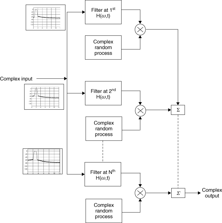
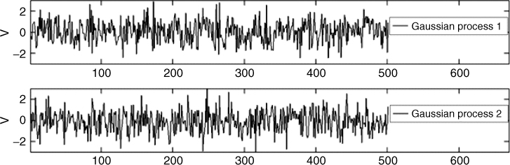
Figure 6.15 Example of complex Gaussian processes representing the gain taps.
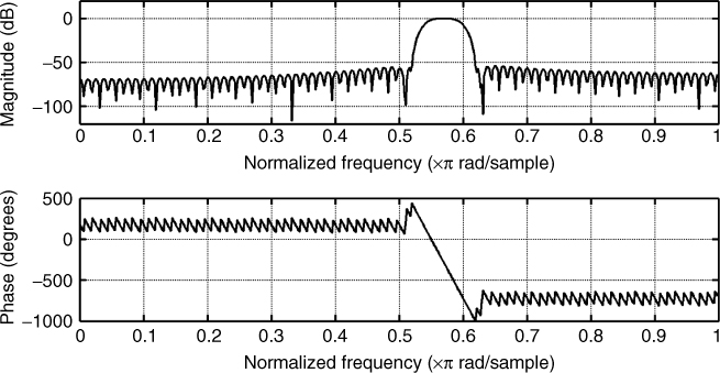
To realize the channel with minimum distortion effects, the filters should have a sharp cut-off, linear phase and minimum ripple in-band and out-of-band. In [27] and [28] FIR filters based on the frequency sampling method were used to realize filters with 160 coefficients using the Hamming window to reduce the sidelobe level. These filters have linear phase, as illustrated in Figure 6.16 for one of the frequency sections.
Figure 6.16 Magnitude and phase frequency response of a filter used to represent one of the frequency sections in Figure 6.14.
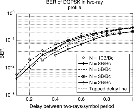
To identify the number of frequency segments needed for the model, in [27] a two-ray channel model assuming that the two rays have equal power and changing the ratio of the differential time delay between the two rays, τd, to the symbol duration, T between 0.1 and 1 was used in a differential quadrature phase shift keying (DQPSK) simulator as in Figure 6.17. The simulations assumed a symbol rate of 24 300, a differential time delay between 4.11 and 41.15 µs and a 40 Hz Doppler spread. When using the relationship introduced by Cavers [29] for a 0.5 correlation coefficient of the coherence bandwidth ![]() , results in a value of
, results in a value of ![]() between 7.74 kHz and 77.4 kHz. Figure 6.18 shows that to obtain the same results as the tapped delay line, the number of branches is equal to N = 10B/Bc = 10πBτmax. For example, for a 350–400 ns RMS delay spread and a 10 MHz bandwidth, the number of branches is between 220 and 251, which is significantly higher than the tapped delay line model.
between 7.74 kHz and 77.4 kHz. Figure 6.18 shows that to obtain the same results as the tapped delay line, the number of branches is equal to N = 10B/Bc = 10πBτmax. For example, for a 350–400 ns RMS delay spread and a 10 MHz bandwidth, the number of branches is between 220 and 251, which is significantly higher than the tapped delay line model.
Figure 6.17 Block diagram of the simulator used to estimate the number of branches needed to estimate the transfer function model.
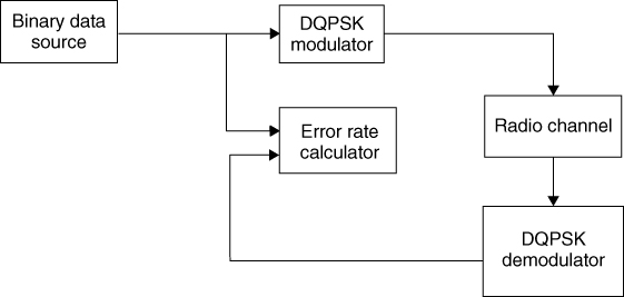
Figure 6.18 Bit error rate computed with different numbers of frequency sections N [27].
Source: Khokhar, K., and Salous, S., (2008), Frequency domain simulator for mobile radio channels and for IEEE 802.16-2004 standard using measured channels, IET Commun., Vol. 2, No. 7, pp. 869–877 doi: 10.1049/iet-com:20070385. Reproduced with permission of IET.
6.4 Frequency Domain Implementation Using Fast Convolution
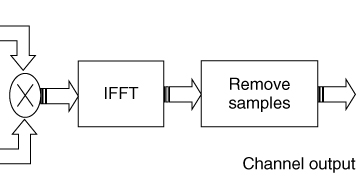
Another implementation of the channel function in the frequency domain is the fast convolution method where the Fourier transform of the channel's impulse response is multiplied by the transmitted signal (channel input) and then transferred back to the time domain using the forward and the inverse Fast Fourier Transform (FFT) as in Figure 6.19. In this method, zero-padding is necessary since the convolution of two signals is equal to the sum of their individual duration. Hence, the length of the FFT for each signal should be greater than or equal to the duration of this sum. The resulting IFFT length is then reduced to match the length of the convolution.
Figure 6.19 Block diagram of frequency domain implementation of convolution.
6.5 Channel Block Realization from Measured Data
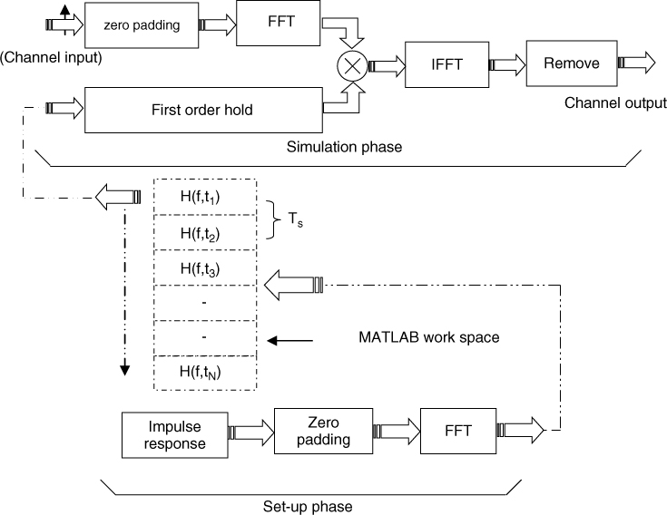
An alternative to predicting link performance from a channel model is to use channel measurements from various scenarios into a simulator using either a direct method or an indirect method. In the direct method, the channel data are entered into the simulator at the rate at which the data were obtained. For example, using the fast convolution method, the channel impulse response can be preprocessed to obtain the frequency domain response, stored into a two-dimensional array as shown in Figure 6.20, which are then entered into a first order hold block updated at Ts, the rate at which the impulse response was originally obtained from the measurements. This is analogous to ‘playing back’ the measured data into the simulator at the correct speed.
Figure 6.20 Playback channel block simulator using the fast convolution method [27].
Source: Khokhar, K., and Salous, S., (2008), Frequency domain simulator for mobile radio channels and for IEEE 802.16-2004 standard using measured channels, IET Commun., Vol. 2, No. 7, pp. 869–877 doi: 10.1049/iet-com:20070385. Reproduced with permission of IET.
In the indirect method the channel data are processed to estimate the channel parameters, which are in turn used in a channel model. For example, in the tapped delay line model, the small-scale channel data are processed to estimate the relative time delay and relative amplitude of the multipath components from the power delay profile. For each ‘multipath component’ the fading distribution such as that of Rayleigh or Rice and the Rician k ratio are estimated as well as the Doppler function, with the corresponding maximum Doppler shift to determine the rate of fading. Depending on the bandwidth of the channel and the system's bandwidth for which the simulations are to be obtained, the data are usually filtered prior to extraction of the channel parameters. For example, channel data obtained to characterize 3 G systems with a 60 MHz bandwidth are filtered down to the 5 MHz bandwidth allocated for each user. A threshold is then applied to the power delay profile to identify the multipath components where the time delay axis is subdivided into time delay bins proportional to the inverse of the bandwidth. In general, a number of simulators assume a small number of multipath components as most communication systems tend to have a restricted bandwidth.
6.6 Theoretical Prediction of System Performance in Additive White Gaussian Noise
In this section, we start by reviewing the two optimum detectors, the matched filter and the correlation detector, and then discuss the error rates in the presence of AWGN, which is representative of thermal noise. We study both optimum and noncoherent detectors for two basic modulation schemes: binary frequency shift keying where the 1 and 0 are represented by two different frequencies and binary phase shift keying where the 1 and 0 are represented by a differential phase shift of 180° and as illustrated in Figure 6.21. We then present system performance for higher order modulation.
Figure 6.21 Waveforms illustrating representation of binary data: (a) frequency shift keying (FSK) signal and (b) phase shift keying (PSK) signal.
6.6.1 Matched Filter and Correlation Detector
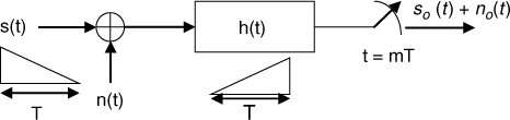
In 1943 D.O. North introduced the concept of the matched filter, which gives optimum performance in the presence of AWGN [30]. As discussed in Section 4.5 on channel sounding and illustrated in Figure 6.22, the matched filter is designed for a specific signal s(t) with duration T. It has an impulse response that is the mirror image of the signal shifted by T to start at t = 0 for causality, as given in:
6.15 ![]()
Figure 6.22 Block diagram of the matched filter.
In the presence of AWGN with zero mean, a variance of ![]() and double-sided spectral density No/2, the filter is designed to maximize the magnitude squared of the signal at the instant of sampling T with respect to the average noise power N; that is:
and double-sided spectral density No/2, the filter is designed to maximize the magnitude squared of the signal at the instant of sampling T with respect to the average noise power N; that is:
The noise component at the output of the matched filter at the instant of sampling can be found either from Equation (4.42) or from the convolution of the noise with the impulse response of the filter given as:
6.17 
The noise power is then found from the ensemble average as in:
Since the power spectrum of noise is flat, its autocorrelation function is an impulse which reduces Equation (6.18) to:
Using Equations (4.47) and (6.19), Equation (6.16) reduces to:
where ![]() is the energy in the signal and for binary data it designates the energy per bit.
is the energy in the signal and for binary data it designates the energy per bit.
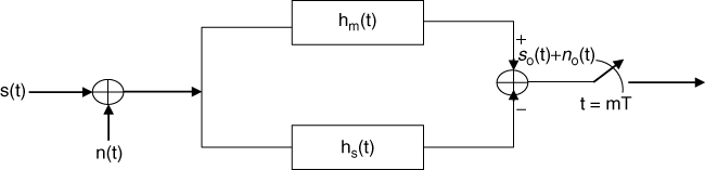
In contrast to channel sounding where usually a single waveform is transmitted, in digital communication at least two waveforms are needed to represent binary data as in frequency shift keying (FSK) modulation, which in general requires two matched filters as in Figure 6.23, where the subscripts m and s represent the mark (binary 1) and space (binary 0) signals respectively. The two outputs of the mark and space matched filters are then compared using a polarity detector to decide which of the two waveforms is received.
Figure 6.23 General matched filter detector of binary data.
Since the two filters would have an output at the instant of sampling, it is desirable to minimize the contribution of the unwanted component. This condition is expressed in terms of the correlation coefficient ![]() between the mark and space signals defined as in:
between the mark and space signals defined as in:
6.20 
where ![]() are the mark and space signals respectively and −1
are the mark and space signals respectively and −1 ![]() . The output due to the signal components at t = T is then given by:
. The output due to the signal components at t = T is then given by:
6.21 ![]()
where the plus and minus signs correspond to the mark and space signals respectively.
The output noise power of the general matched filter can be shown to be equal to ![]() . Thus, substitution of Equation (6.22) into Equation (6.16) results in:
. Thus, substitution of Equation (6.22) into Equation (6.16) results in:
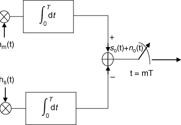
An alternative to the matched filter is the correlation detector, shown in Figure 6.24 where the received signal is multiplied by a stored replica and integrated over the bit duration. Although the two techniques give identical results at the correct sampling instant, the waveforms at the output of the detectors at any other instant in time are different. In both detectors, it is necessary to have bit synchronization for sampling the output at the correct instant in time, to ensure optimum detection.
Figure 6.24 Block diagram of correlation detector.
6.6.2 Bit Error Rate of the Matched Filter Detector in AWGN
Detailed analysis of the theoretical BERs for various modulation schemes, including higher order modulation, can be found in numerous textbooks, such as that of Proakis [31]. To illustrate the analysis of the error rate we will derive the expression for the single matched filter detector in Figure 6.22, which can be used for antipodal data transmission such as for phase shift keying (PSK). Generally, errors in data transmission occur in one of two cases: transmitting a mark signal and detecting a space signal, and transmitting a space signal and detecting a mark signal. Thus the BER can be found from Equation (6.1), which is usually computed as a function of the energy per bit Eb to No.
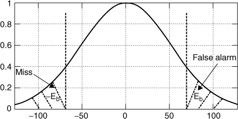
Figure 6.25 shows the Gaussian probability density function of noise where the shaded areas indicate the regions of error. These are the areas where a mark has been transmitted and the noise voltage exceeds –E (probability of a miss) or when a space has been transmitted and the noise is in excess of E (probability of a false alarm). Hence the probability of error is given by:
6.23 ![]()
Figure 6.25 Gaussian PDF representing noise and threshold levels indicating error regions.
where p(m) and p(s) correspond to the probability of transmitting a mark or a space signal respectively.
In data transmission, the mark and space are likely to be generated with equal probability. Hence the probability of error reduces to:
6.24 
Using the complementary error function, erfc(x), and the error function, erf(x), and using substitution of variables, the probability of error can be expressed as in:
6.26b 
Equation (6.26c) follows from the standard deviation of noise ![]() being the RMS value of noise voltage, which if it passes through a 1 Ω resistor would give rise to a noise power N. Using Equation (6.19), the BER in Equation (6.26a) can be expressed as in:
being the RMS value of noise voltage, which if it passes through a 1 Ω resistor would give rise to a noise power N. Using Equation (6.19), the BER in Equation (6.26a) can be expressed as in:
6.27 
Similar analysis can be carried out for the general matched filter of Figure 6.23 to estimate the probability of error of data transmission, which requires two different waveforms such as for the case of FSK. In this case the threshold lines in Figure 6.25 are set to ![]() , which gives the theoretical expression for the probability of error:
, which gives the theoretical expression for the probability of error:
6.28 
6.6.3 Bit Error Rate with Noncoherent Detectors
The optimum correlation detector in Figure 6.24 requires timing synchronization and phase coherence with the incoming signal, which can be difficult to achieve. This requirement can be relaxed using suboptimum receivers. For example, for FSK transmissions two separate bandpass filters for the mark and space signals followed by envelope detectors can be used to identify the received data sequence. For this type of detector it is necessary to ensure that the frequency separation between the mark and space signals is significantly large to enable appropriate filtering. The theoretical probability of error for such a detector is given by:
6.29 ![]()
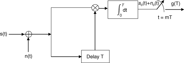
In the case of PSK, it is possible to derive the reference from the received signal using differential encoding, which is referred to as differential phase shift keying (DPSK) (introduced ∼1955). To enable the derivation of the reference signal, the coding starts with a reference bit, say a mark bit, and phase changes occur when the bit is a space signal. For example, a sequence of bits {1 0 1 1 0 1 0 0 1} would be differentially encoded as {(1) 1 0 0 0 1 1 0 1 1}. By correlating the incoming signal with a delayed version of itself effectively compares the phase of the incoming bit with the previous bit. For this example a mark is detected if the phase of the incoming bit is identical to the previous one and a space bit is detected if they are out of phase. This gives rise to the detector shown in Figure 6.26 with a probability of error as given by:
6.30 ![]()
Figure 6.26 Block diagram of differential phase shift keying.
6.6.4 Comparison of BER of Coherent and Noncoherent Detectors
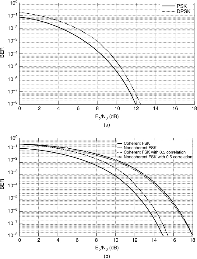
Figure 6.27a and b compares the theoretical BER curves obtained using the BER tool in Matlab of both coherent and noncoherent detectors of PSK and FSK signals where it is seen that the degradation in performance of DPSK is less than 1 dB in comparison to PSK with ideal detection, which makes it an attractive option. Similarly, the degradation of the noncoherent FSK detector is also less than 1 dB as shown in Figure 6.27b for both orthogonal FSK, that is for the zero correlation coefficient and for the case of 0.5 correlation.
Figure 6.27 BER curves for coherent and noncoherent detectors: (a) PSK and (b) FSK.
6.6.5 Higher Order Modulation
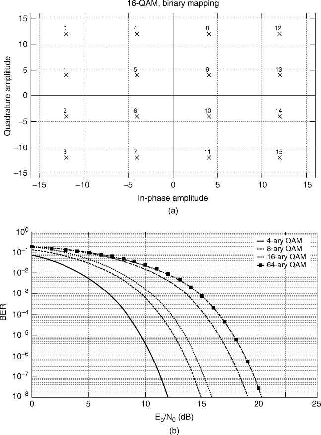
To enable the transmission of higher data rates, each transmitted symbol comprises 2n bits, where n is an integer and the resultant modulation is referred to as M-ary modulation. For example, for n = 2, every two bits are combined to form a symbol, and the resulting M = 4 combinations are encoded using any of the standard modulation techniques of phase, frequency or amplitude. This is achieved by generating a complex vector where each symbol is represented by a combination of in-phase and quadratue components as illustrated in Figure 6.28a for the rectangular 16-ary QAM. The corresponding error rate obtained with the BER tool of Matlab for different M-ary ranging from 4-ary to 64-ary QAM is shown in Figure 6.28b, where for the same energy per bit to noise ratio, higher error rates are experienced for higher modulation.
Figure 6.28 (a) Constellation of 16-ary QAM and (b) BER for 4-ary, 8-ary, 16-ary, 32-ary and 64-ary QAM versus energy per bit to noise ratio.
Since a number of bits make up a symbol, it is usual to give the theoretical symbol error rates versus the symbol energy ![]() to noise ratio, instead of the BER versus the energy per bit to noise ratio, where:
to noise ratio, instead of the BER versus the energy per bit to noise ratio, where:
6.31 ![]()
and the relationship between the binary error rate and the M-ary error rate is approximately given by:
6.32 ![]()
The expressions for the BERs for the different M-ary modulations ![]() can be found in [31] to [33], which are given in:
can be found in [31] to [33], which are given in:
6.33a 
6.33b 
where
6.33c 
The corresponding relationship for noncoherent detection of M-ary FSK is given in:
6.34 ![]()
6.7 Prediction of System Performance in Fading Channels
In this section we study the effect of multipath on data transmission. Two types of fading will be considered: narrowband fading where the signal bandwidth is much smaller than the coherent bandwidth of the channel and wideband transmission where the signal bandwidth is in excess of the coherent bandwidth of the channel. Theoretical BERs are compared with stochastic models where it is appropriate to use the BER tool in the Matlab SIMULINK environment.
6.7.1 Narrowband Signals
In the narrowband case, all the frequency components suffer from the same attenuation. The received signal goes through maxima and minima at a rate determined by the maximum Doppler shift or equivalently the coherent time of the channel.
The theoretical error rates for PSK, FSK, DPSK and noncoherent FSK in a slow fading Rayleigh environment are given in the following equations (see [31], Chapter 14.3, p. 774):
6.35a 
6.35b 
6.35c ![]()
6.35d ![]()
where
6.36 ![]()
and ![]() is the expected value of a chi-square probability distribution with two degrees of freedom and
is the expected value of a chi-square probability distribution with two degrees of freedom and ![]() is Rayleigh distributed. The theoretical probabilities of error curves are illustrated in Figure 6.29.
is Rayleigh distributed. The theoretical probabilities of error curves are illustrated in Figure 6.29.
Figure 6.29 Theoretical bit error rate for basic modulation schemes in a Rayleigh fading channel.

The effect of fading on the BER is illustrated in Figure 6.30, which compares the error rate for the case of PSK in AWGN with fading channels for different Rician k-ratios and for Rayleigh fading. A k ratio of 100 is seen to give close to the ideal BER whereas a k ratio of 10 still gives a 15 dB advantage with respect to Rayleigh fading at error rates of 1 in 10−3.
Figure 6.30 Bit error rate for PSK modulation in AWGN, a Rayleigh fading channel and a Rice fading channel with k ratios: 10, 20, 50 and 100.
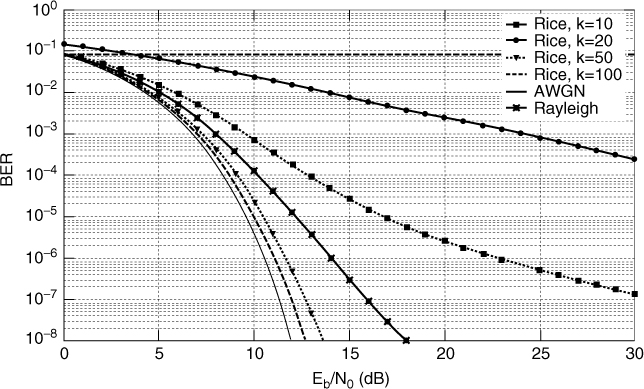
Figure 6.31a displays a typical SIMULINK set-up for the estimation of error rate for different modulation schemes using different types of channels. Narrowband channel models usually consist of a single Rayleigh or Rician fading path with typical parameters such as the Rice k ratio, maximum Doppler shift, the shape of the Doppler spectrum and any initial phase shift. In [34] the Rayleigh fading generator is used to show the coincidence of the stochastic and the theoretical BER curves for the example of BPSK. In the simulations the channel model, which can be represented as in Figure 6.31b, can be expressed as:
Figure 6.31 (a) Block diagram of a SIMULINK set-up for the computation of the error rate including the channel effects and (b) narrowband block diagram representing the channel as in Equation (6.37).
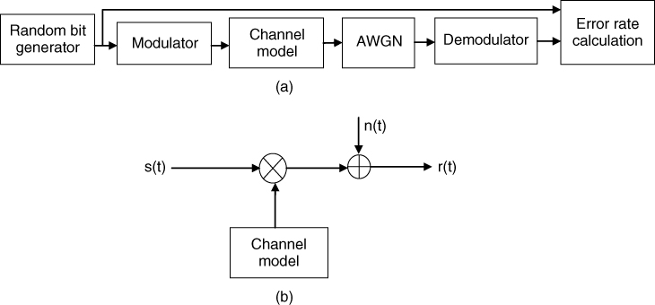
where ![]() is assumed to be Rayleigh distributed with a mean square value of 1 and
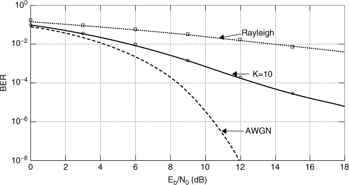
is assumed to be Rayleigh distributed with a mean square value of 1 and ![]() . The phase component is neglected assuming coherent detection. The Rician error rate can be obtained in a similar manner by replacing the Rayleigh distribution with a Rician distribution with the appropriate k ratio. Figure 6.32 compares the theoretical and stochastic error rates obtained for both Rayleigh and Rician fading with k = 10.
. The phase component is neglected assuming coherent detection. The Rician error rate can be obtained in a similar manner by replacing the Rayleigh distribution with a Rician distribution with the appropriate k ratio. Figure 6.32 compares the theoretical and stochastic error rates obtained for both Rayleigh and Rician fading with k = 10.
Figure 6.32 Bit error rate for theoretical responses of PSK in AWGN, Rayleigh fading and Rician fading, with squares and circles indicating stochastic simulations.
6.7.2 Wideband Signals
In the wideband case the signal bandwidth exceeds the coherent bandwidth of the channel and hence the different frequency components suffer from frequency selectivity. These effects are generally modelled using the tapped delay line impulse response model given in the following equation, where each multipath component has its own amplitude and phase distribution, which are considered to be independent:
6.38 
For many applications it is sufficient to use the two-ray model which consists of the first two terms to illustrate the relationship of the time delay difference between the two components and the BER. By changing the time delay between the two components with respect to the symbol duration, the effect of frequency selectivity can be estimated. The path gains are generally assumed to be independent Rayleigh distributed with uniform phase distributions over [0 2π]. One or both path gains can also be assumed to be Rician distributed. An example of the effect of a two-ray multipath channel on DPSK was previously shown in Figure 6.18 for different separation between the two rays with respect to the symbol period. Figure 6.18 shows that as the separation between the two multipath components increases with respect to the symbol period, the BER also increases.
The effects of frequency selectivity induced by the presence of multipath are normally reduced using diversity techniques, which include frequency, time, space and polarization diversity (see Section 6.9). Various coding techniques such as Reed Solomon and convolution encoders can also be applied to reduce the BER as discussed in Section 6.8.
Another method of combating multipath is to use the RAKE receiver first proposed by Price and Green in 1958 [35] for spread spectrum modulation where the data generated at a low rate are spread over a wider bandwidth (BW), which is in excess of the coherence bandwidth of the channel, using coded transmission such as a pseudorandom code or a Gold code. At the receiver, a correlation detector with a synchronized replica of the code is used to compress the bandwidth of the received signal. The technique resolves the multipath components with a time delay resolution equal to 1/BW, and for a maximum time delay spread of Tm the number of resolvable paths is BW Tm. At the receiver, the resolved replicas are then combined coherently to enhance the SNR using several detectors, as illustrated in Figure 6.33a where the delays τi are set to correspond to the differential time delay between the multipath components as shown in Figure 6.33b. Aligning the outputs of the detectors in time and taking the sum provides multipath diversity gain which enhances the received signal to noise ratio (SNR). This technique is implemented in third generation mobile radio systems discussed in Section 6.8.3, where the methods of diversity combining are discussed in Section 6.9.
Figure 6.33 (a) Architecture of RAKE receiver and (b) multipath structure as a function of time where the arrows indicate the multipath components and their delays into the receiver.
6.8 Bit Error Rate Prediction for Wireless Standards
A wide variety of wireless technologies are available on the market that provide coverage in various environments such as the wireless local area network (WLAN), wireless personal area networks (WPANs) and wireless metropolitan area networks (WiMANs). These networks are defined by standards that determine the different types of modulation, coding and data rates used in the standard. Examples of standards are the IEEE 802.11 for WLAN, IEEE 802.15 for vehicular communication, the IEEE 802.16 standard for WiMAN, which is also known as WiMAX, and the third generation cellular system using WCDMA. As examples of the effects of the radio channel on sophisticated communication systems, we will study in this section the BER performance of three standards: the IEEE 802.16-d standard used in the metropolitan fixed wireless access networks and the IEEE 802.11-a standard for WLAN and WCDMA.
6.8.1 IEEE 802.16-d Standard
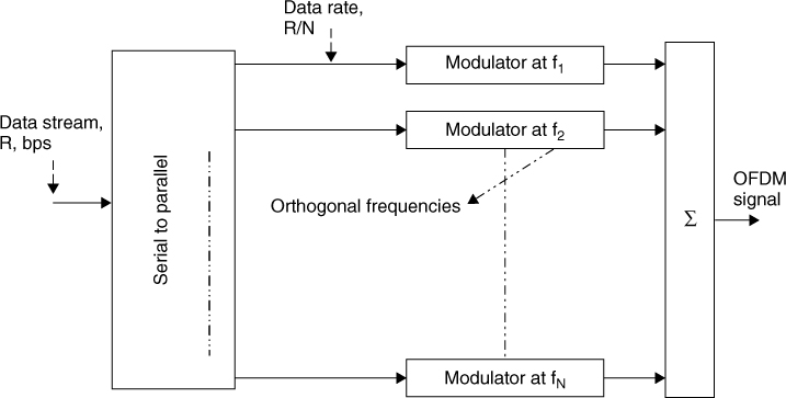
The standard uses orthogonal frequency division multiplexing (OFDM), where the high rate data to be transmitted are divided over a number of carriers that carry data at a lower rate than the original data stream. Thus, in the OFDM modulator the data stream is converted from serial into parallel streams, which are equal to the number of carriers N, as illustrated in Figure 6.34. This increases the symbol duration in each parallel channel, which reduces intersymbol interference (ISI) and mitigates the effects of frequency selective fading. Each parallel stream at the lower band rate is then modulated separately and the summation of all the outputs of the modulators results in the OFDM signal.
Figure 6.34 Conceptual block diagram of an OFDM modulator.
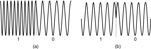
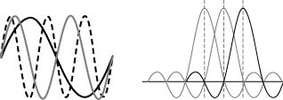
Thus, in OFDM the bandwidth of transmission is divided between a number of carriers chosen such that in each symbol period each carrier has an integer number of cycles and adjacent carriers differ by one cycle as illustrated in Figure 6.35a. The carrier spacing is equal to the reciprocal of the OFDM symbol period, which makes the carriers orthogonal to each other despite their overlap, with the nulls from adjacent carriers coinciding with the centres of neighbouring carriers as illustrated in Figure 6.35b. At the receiver, the individual carriers can be recovered from the overlapped spectrum provided orthogonality is preserved after transmission through the channel.
Figure 6.35 OFDM signal: (a) time domain and (b) frequency domain.
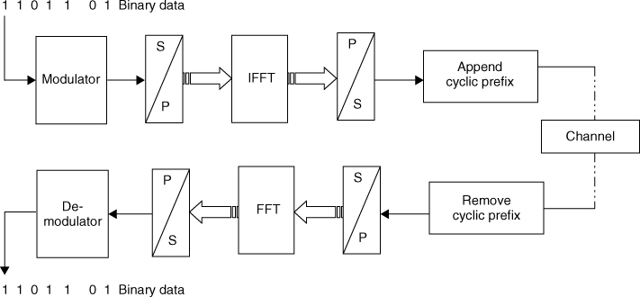
However, in practice OFDM modulation/demodulation is efficiently implemented via the IFFT/FFT. Figure 6.36 gives the block diagram of an OFDM modulator with FFT implementation. Since convolution of the signal with the channel response extends the duration of the signal, a cyclic prefix (CP) is added at the end of the symbol which is then removed at the receiver. The resulting OFDM symbol period Ts is then equal to Tb + Tg, where Tg is the CP time.
Figure 6.36 Block diagram of the OFDM system.
Adaptive modulation ranging from simple BPSK to the 64-level QAM are used in the standard depending on the received SNR. The drop in the signal strength below the noise level due to multipath fading introduces bursts of errors in the data, which are combated by using coding with different rates. Channel coding involves rearranging and adding redundant data bits prior to transmission and complementary operation at the receiving end. For example, in the IEEE 802.16-2004 standard, channel coding is achieved in three steps: randomization, forward error correction (FEC) and interleaving. Randomizers toggle some of the zeros to ones or ones to zeros to avoid long strings of ones and zeros. This optimizes the decision regions of a maximum likelihood detector in the receiver. FEC codes add extra bits to the original data at the expense of an increase in bandwidth. They detect and correct errors at the receiver without requesting retransmission. FEC codes are classified into block codes such as Reed–Solomon (RS) codes, which can handle burst errors, and convolution codes, which handle random errors. The IEEE 802.16-2004 standard employs concatenated Reed–Solomon encoder/decoder and convolution encoder/decoder, which provide large coding gain with less implementation complexity as compared to a single coding scheme [36]. The encoded data are then scrambled by the interleaver prior to transmission to combat the effects of the fading channel which might introduce a burst of correlated bit errors. At the receiving end, the de-interleaver rearranges the data to its original order, thus distributing a series of errors which can be corrected by the FEC schemes.
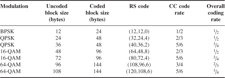
To achieve different coding rates, puncturing that removes some of the parity bits is employed. For example, the native rate 1/2 encoder employed in the IEEE 802.16 standard is punctured to give coding rates equal to 1/2, 2/3 and 3/4. Figure 6.37 shows the overall encoder employed in the standard and Table 6.1 gives details of the uncoded and coded block sizes, the Reed–Solomon code, the convolution code rate and the resulting overall coding rate. The RS encoder is specified as RS (N, K, T), where N and K refer to the number of the overall bytes after and before encoding respectively and T denotes the number of data bytes that can be corrected. The convolution encoder maps each k bit of continuous input stream on to n output bits by convolving the input bits with a binary impulse response. This is achieved with an M stage shift register and n modulo-2 adders to generate the redundant bits. A convolution encoder is characterized by the constraint length J, generator polynomials and code rate R. The constraint length indicates the number of shifts over which a single message bit enters and leaves the shift register.
Figure 6.37 Block diagram of an overall encoder in the IEEE 802.16 standard.

Table 6.1 Coding requirements for various modulation schemes for IEEE 802.16-2004 standards
The standard employs 256 carriers where 192 carriers are used for data transmission, 8 carriers for pilot tones at frequency offsets of ±12, ±36, ±60 and ±84 for tracking, channel estimation and frequency offset estimation, 55 carriers for guard bands and a DC component as illustrated in Figure 6.38.
Figure 6.38 Distribution of carriers in the IEEE 802.16 standard: (a) pilot carriers and (b) data and guard carriers.
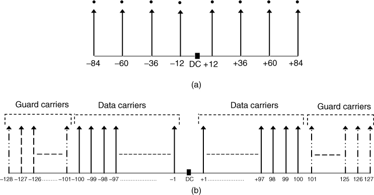
Prior to transmission, the data are structured into frames where each subframe is always preceded by a preamble, which comprises one or more OFDM symbols of known values. Preambles are used for synchronization between the transmitter and the receiver and for channel estimation. The uplink preamble, referred to as a short preamble, contains 100 QPSK carriers at even numbered locations and consists of two times 128 samples preceded by a CP as shown in Figure 6.39a. The downlink preamble, referred to as a long preamble, is shown in Figure 6.39b. It is equivalent to two OFDM symbols and consists of a CP and four times 64 samples followed by a CP and two times 128 samples, where the first symbol of this preamble uses 50 subcarriers (every fourth subcarrier of the available 200) and the second symbol uses 100 subcarriers (all at even numbered positions). All subcarriers in the long preamble are QPSK modulated.
Figure 6.39 Preambles used in (a) uplink and (b) downlink.
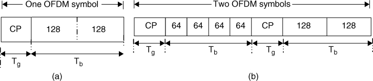
Figure 6.40 gives the overall diagram of the implementation of the standard that can be used to set up a simulator to predict the performance of the standard in the presence of AWGN and channel impairments. This can be enabled through a channel function that can be realized either in the time domain using the tapped delay line method or in the frequency domain using FFT and IFFT. The standard allows different bandwidths in the licensed bands with multiples of 1.75 MHz channel bandwidths, and in the licensed exempt band multiples of 8/7 and 7/6 up to 20 MHz bandwidth. To enable testing of the modulation schemes and different coding rate the simulator needs to be reconfigurable and adaptive such that the modulation schemes with the corresponding FEC rates are changed according to SNR threshold levels. Such a simulator based on the tapped delay line model is available from Matlab SIMULINK Communications Block demonstrators whereas the frequency domain model of the channel is reported in [27].
Figure 6.40 Block diagram of the IEEE 802.16 standard simulator.
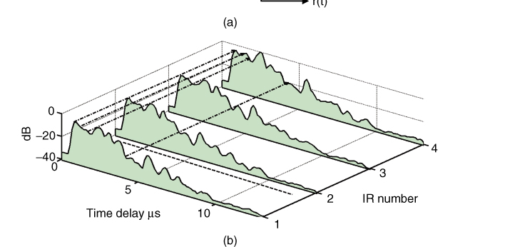
Performance of the standard can be evaluated either using standard channel models such as the Stanford University Interim (SUI) models or from measured data in the environment of interest. In the time domain channel model information regarding multipath components, such as their relative time delay, their relative amplitude, their Doppler spectra including the maximum expected Doppler shift and the Rician k-factor, form the input into the simulator. This requires specifying a particular number of taps, which in most commercial simulators is limited to four taps. The tap amplitude and relative time delay are extracted from the average power delay profile as illustrated in Figure 6.41a for three power delay profiles acquired simultaneously at three frequencies, 2.5 GHz, 3.5 GHz, and 5.8 GHz, at two locations processed with a 2.56 MHz resolution bandwidth. The k-factor is extracted from the time-variant impulse response for each tap, which represents a ‘group’ of multipath components that is a subset of the overall number of the received multipath components.
Figure 6.41 (a) Average power delay profile in two locations measured in a rural area in the UK at three frequencies representative of the environment for the installation of the IEEE 802.16 standard and (b) corresponding time-variant frequency channel function used in a frequency domain simulator [27].
Source: Khokhar, K., and Salous, S., (2008), Frequency domain simulator for mobile radio channels and for IEEE 802.16-2004 standard using measured channels, IET Commun., Vol. 2, No. 7, pp. 869–877 doi: 10.1049/iet-com:20070385. Reproduced with permission of IET.

For quasi-stationary measurements, as for fixed wireless access networks where the time variations are caused mainly by the movement in the environment rather than the terminal, the k-factor can be extracted by converting the two-dimensional time-variant transfer function into a single dimensional matrix.
Using the frequency domain ‘playback’ channel simulator the time-variant frequency response of the channel data as shown in Figure 6.41b can be entered into the simulator. Since 256 carriers are used in the standard, zero padding to 512 points is introduced to permit using the FFT in the implementation of the channel block. Hence the frequency axis shows 512 frequency points, whereas the time axis shows 250 impulse responses acquired at 4 ms intervals, which give a total observation time of 1 second. The profiles are seen to exhibit different frequency selectivity properties and a slow Doppler rate, as would be expected for fixed wireless access links.
Figure 6.42 displays the BER for the two locations for 16-QAM modulation with ½ rate coding where location 1 shows a significantly higher error rate than location 2.
Figure 6.42 BER for 16-QAM modulation with ½ rate coding in (a) location 1 and (b) location 2 of Figure 6.41 [27].
Source: Khokhar, K., and Salous, S., (2008), Frequency domain simulator for mobile radio channels and for IEEE 802.16-2004 standard using measured channels, IET Commun., Vol. 2, No. 7, pp. 869–877 doi: 10.1049/iet-com:20070385. Reproduced with permission of IET.
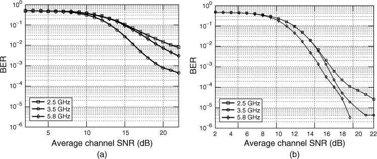
The BER can be related to the channel frequency selectivity. For example, in location 1 the 2.5 GHz band has more minima across the bandwidth, followed by the 5.8 GHz band, which has deep minima on the edges of the band with the best performance achieved in the 3.5 GHz band. The increase in error rate is due to the puncturing used in the error correction code. Comparing the BER curves for the profiles in location 2, a lower error rate is observed, which is consistent with the lower frequency selectivity.
6.8.2 IEEE 802.11-a Standard
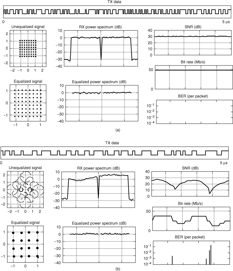
Similar to the WiMAX standard, the IEEE 802.11-a standard also uses convolutional coding and puncturing with code rates of 1/2, 2/3 and 3/4, data interleaving and BPSK, QPSK, 16-QAM and 64-QAM modulation and variable data rates as given in Table 6.2. It uses OFDM transmission with 52 subcarriers, 4 pilots, 64-point FFT and a 16-sample CP. A SIMULINK model of the standard, which includes adaptive data rate transmission to accommodate the channel effects, is available from the Matlab Communications Block demonstrators. The channel block used in the simulator is based on the tapped delay line and provides three options: no fading, that is AWGN only, flat-fading with maximum Doppler shift and frequency dispersive channel with two multipath components. Figure 6.43 illustrates the relationship between the data rate and the drop in the SNR and shows the modulation constellation prior to and after equalization for a flat fading channel with a 200 Hz Doppler shift. Figure 6.44 contrasts the effect of a ‘frequency dispersive’ channel with two components with the second component at −3 dB relative to the first component and 200 Hz maximum Doppler shift to the ‘no fading’ channel for a 30 dB SNR level . The simulation result shows a steady state of 54 Mbps for the ‘no fading’ channel with variable data rate for the frequency selective channel.
Table 6.2 Modulation, coding rate and corresponding data rate of the standard
| Modulation | CC code rate | Data rate (Mb/s) |
| BPSK | 1/2 | 6 |
| BPSK | 3/4 | 9 |
| QPSK | 1/2 | 12 |
| QPSK | 3/4 | 18 |
| 16-QAM | 1/2 | 24 |
| 16-QAM | 3/4 | 36 |
| 64-QAM | 2/3 | 48 |
| 64-QAM | 3/4 | 54 |
Figure 6.43 Transmitted binary data, with the correspoding equalized and unequalized channel in the presence of additive white Gaussian noise and flat fading, and the data rate in relation to the SNR.
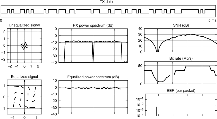
Figure 6.44 Simulation results of the IEEE802.11 standard performance in (a) an AWGN channel and (b) a frequency selective channel.
6.8.3 Third Generation WCDMA Standard
WCDMA is one of five air interfaces for third generation wireless communications developed within the framework of the International Mobile Telecommunications (IMT)-2000, as defined by the International Telecommunication Union (ITU). The specifications of WCDMA are developed by the Third Generation Partnership Project (3GPP), which is a joint effort among standards bodies from Europe, Japan, Korea, the USA and China.
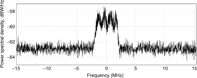
The WCDMA air interface is a spread spectrum multiple access technology that spreads the encoded user data generated at a low rate as shown in Figure 6.45a over a wider bandwidth as illustrated in Figure 6.45b using a pseudorandom sequence clocked at a chip rate equal to 3.84 Mcps. Orthogonal Variable Spreading Factor codes are used with 4–256 spreading factor for the uplink and 4–512 spreading factor for the downlink. This gives a processing gain, which is defined as the ratio of the spread data rate (3.84 Mcps) to the initial data rate, and a spreading gain, which is the ratio of the spread data rate to the encoded data rate. By assigning a unique code to each user, the receiver, which has knowledge of the code of the intended user, can successfully separate the desired signal from the received waveform. The standard permits different data rates ranging from 9.6 kb/s for satellite users, 144 kb/s for vehicular users, 384 kb/s for pedestrian users and 2.048 Mb/s for an indoor office environment. In order to address higher data rates high speed downlink packet access (HSDPA), which allows data rates of up to 10 Mbps (and 20 Mbps for multiple input–multiple output (MIMO) systems) and is based on 16-QAM modulation, has been introduced into release 5 of the WCDMA (3GPP) standard. HSDPA is only available in the downlink direction, which makes it ideal for loading large e-mails, surf the Web or download videos. Table 6.3 gives the data rate, modulation and MIMO configurations as proposed in release 6 and releases 7 to 9. A RAKE receiver is used to combat the effects of multipath that cause frequency selectivity as seen in Figure 6.46.
Figure 6.45 (a) Spectrum of baseband data prior to encoding and (b) spectrum of data following spreading.
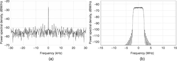
Table 6.3 Data rate, modulation type and MIMO configurations as proposed by 3GPP releases 6 and 7 to 9
| 3GPP release 6 | 3GPP release 7/8/9/10 (HSPA+) | |
| (WCDMA/HSPA) | ||
| Modulation | DL: QPSK, 16QAM | DL: QPSK, 16QAM, 64QAM |
| UL: dual BPSK | UL: dual BPSK, 16QAM | |
| MIMO mode | — | DL: 2 × 2 |
| UL: 1 × 2 | ||
| Peak data rate | WCDMA (DL, UL): 384 kbit/s | DL: 28 Mbit/s (MIMO, 16-QAM) |
| HSDPA (DL): 14.4 Mbit/s | DL: 42.2 Mbit/s (MIMO, 64-QAM) | |
| HSUPA (UL): 5.76 Mbit/s | DL: 42.2 Mbit/s (64-QAM, dual carrier) | |
| DL: 84.4 Mbit/s (MIMO, 64-QAM, dual carrier) | ||
| UL: 11.5 Mbit/s (16-QAM) | ||
| UL: 23 Mbit/s (16-QAM, dual carrier) |
Figure 6.46 Spectrum of a spread signal after passing through the multipath channel.
Carrier spacing is on the order of 4.2–5 MHz, as seen from Figure 6.47 from the spectrum of the downlink band as received with a spectrum analyzer. The standard uses Turbo coding and convolution coding with rates of ½ and 1/3. A SIMULINK model of release 99, which is the first release of the standard, is available from the Communications Block demonstrator in Matlab and can be used to estimate the error rate of the downlink with the channel models recommended by the 3GPP as given in Table 6.4, which includes a maximum of four multipath components and user speeds ranging from 3 km/h to 250 km/h. The number of multipath components corresponds to the number of ‘fingers’ in the RAKE receiver.
Figure 6.47 Spectrum of downlink as measured on a spectrum analyzer.
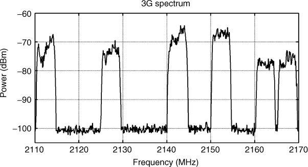
Table 6.4 Multipath channel models as recommended by the 3GPP for WCDMA for different vehicular speeds
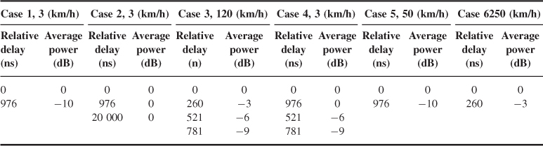
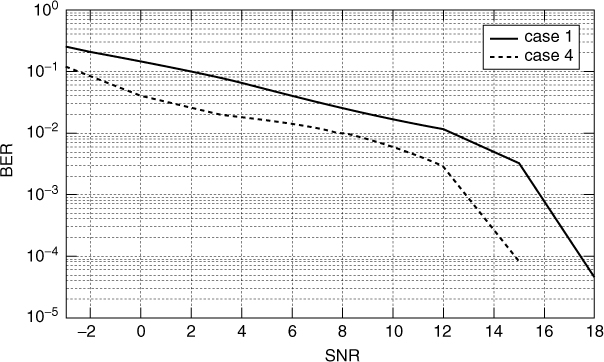
The BER for the downlink assuming 384 kbps at 3 km/h is shown in Figure 6.48 for cases 1 and 4 in Table 6.4, which have two multipath components at similar delay but in case 4 the two components have equal power. Thus, when combined they result in a lower error rate, which at a BER of 1 × 10⁻³ gives a 3 dB advantage.
Figure 6.48 Bit error rate for WCDMA assuming 384 kbps at 3 km/h for case 1 and 2 multipath models given in Table 6.4.
6.9 Enhancement of Performance Using Diversity Gain
Diversity aims to alleviate the errors that occur due to signal fading by combining independent fading versions of the same signal. The assumption is that if the probability of one signal level being below a certain threshold is p, then the probability of L independent signals all being below the same threshold is pL. Thus by combining independently fading replicas of the same signal, the SNR can be enhanced to reduce the BER. The independent fading signals can be obtained by transmit or receive diversity.
Diversity can be realized using any of the following techniques:
- Frequency diversity;
- Polarization diversity and field diversity;
- Time diversity;
- Space diversity using different antennas; and
- Multipath diversity (tapped delay line equalizer, RAKE receiver).
In order to set up a diversity system, it is therefore necessary to identify the coherence parameters of the channel, which include the coherence time, the coherence distance and the coherence bandwidth. For example, in frequency diversity, the same information is transmitted over a number of carriers, which are separated by at least the coherence bandwidth. This has a major drawback in mobile radio channels operating in the UHF band where the coherent bandwidth can be on the order of megahertz and since the spectrum is a valuable resource it is difficult to allocate multiple frequencies per user. Similarly, time diversity repeats the transmission of the same information from the same antenna at time instants that are separated by at least the coherence time of the channel T > (1/2fm) = λ/2ν, where 2fm is the maximum baseband fade rate. Since the message needs to be repeated, time diversity reduces the data throughput rate, but there is no requirement for either co-phasing or duplication of radio equipment. For example, for a mobile speed of 48 km/h and a 900 MHz carrier frequency the required time separation is 12.5 ms, which increases as the fade rate decreases and goes to infinity when the speed is zero. However, at UHF the wavelength is so small that minor movements of people and objects ensure that the channel is never truly stationary.
In space diversity signals from two or more antennas physically separated from each other by at least the coherence distance form the independent samples. This technique is an attractive and a convenient method of diversity reception for mobile radio in the UHF band where the wavelength is a few cm and antenna separations can be accommodated. The necessary antenna separation can easily be obtained at base stations with about 10λ and, assuming isotropic scattering at the mobile end of the link, the autocorrelation coefficient of the envelope of the electric field falls to a low value at distances greater than about a quarter-wavelength, usually λ/2.
An alternative form of antenna diversity relies on using antennas with different polarizations or on field diversity that relies on the electric and magnetic fields being independent. Polarization diversity relies on the scatterers to depolarize the transmitted signal and field diversity uses the fact that the electric and magnetic components of the field at any receiving point are uncorrelated. Both of these methods have their difficulties, since there is not always sufficient depolarization along the transmission path for polarization diversity to be successful and there are difficulties with the design of antennas suitable for field diversity.
6.9.1 Diversity Combining Methods
Diversity reception relies on receiving two or more versions of the incoming signal, which have low, ideally zero cross correlation. Although it is desirable that the correlation coefficient should be very small, it has been shown that full benefits of a diversity scheme can still be realized with correlation coefficients as high as 0.7. These versions (also known as branches) are combined in a suitable manner to produce a signal, which has a lower probability of being below a particular threshold level. In linear diversity combining, the various signal inputs are individually weighted and then added together either after detection in a postdetection combiner or before detection in a predetection combiner. In a predetection combiner the signals are co-phased before addition. Assuming that any necessary processing of this kind has been done, we can express the output of a linear combiner consisting of M branches as:
6.39 ![]()
where sk(t) is the envelope of the kth signal to which a weight ak is applied.
Usually the analysis of combiners is carried out in terms of either the carrier to noise ratio (CNR) or SNR, with the following assumptions [37, 38]:
Different types of combiners can be realized depending on the choice of ak. Three basic combiners are discussed here, which include: scanning and selection combiners (SCs), equal-gain combiners (EGCs) and maximal ratio combiners (MRCs). These are illustrated in Figure 6.49. Equal-gain and maximal ratio combiners accept contributions from all branches simultaneously. In equal-gain combiners all ak are unity whereas in maximal ratio combiners EGC and MRC rely on the coherent addition of the signals against the incoherent addition of noise. This means that when assumptions 1 to 4 hold, both EGC and MRC combining methods show a better performance than scanning or selection combining. As is discussed in Section 6.9.1.1 to 6.9.1.3.
Figure 6.49 Block diagram illustration of (a) selection diversity, (b) maximal ratio combining and (c) equal-gain combining diversity.

6.9.1.1 Scanning and Selection Diversity
In scanning and selection combiners, assumptions 2 and 3 are not used. In such combiners only one input is selected and all other inputs are discarded according to a preset threshold or according to the best short term CNR. In scanning diversity the input signals are scanned sequentially until the input that is greater than the threshold is found. The receiver continues to use that signal until it drops below the threshold, when the scanning procedure restarts. In selection diversity the branch with the best short term CNR is always selected. Assuming that the input signals in each branch are uncorrelated Gaussian processes of equal mean power the PDF of their envelope is Rayleigh fading and can be expressed as:
6.40 ![]()
where
![]()
The resulting mean CNR at the output of the selector ![]() can be shown to be expressed as [38]:
can be shown to be expressed as [38]:
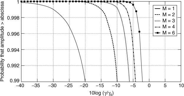
To identify the number of branches to use in SC, the cumulative probability distribution of the best signal taken from M branches being less than or equal to the threshold level ![]() can be used [38], given as:
can be used [38], given as:
6.42 ![]()
If a single branch achieves a CNR ![]() then the corresponding probability is given by:
then the corresponding probability is given by:
A plot of Equation (6.43) is displayed in Figure 6.50. For a 99 % confidence level, the figure shows that a 10 dB advantage can be achieved by increasing the number of diversity branches from one to two. However, the advantage of going from 2 to 6 is only ∼7 dB.
Figure 6.50 Cumulative distribution graph of CNR of selection diversity.
6.9.1.2 Maximal Ratio Combining
In this method, ak is proportional to the root mean square signal and inversely proportional to the mean square noise in the kth branch. As shown in Figure 6.49, it is assumed that the signals from the different branches have been co-phased before combining. Assuming that this has been done, the envelope of the combined signal is given by:
with the corresponding noise power by:
Using Equations (6.44) and (6.45) and the weights are in the ratio of the signal voltage to noise power, that is ak = rk/N, then γR, the SNR, can be maximized and can be shown to be as given by:
where ![]() is the CNR of the kth branch [38]. Equation (6.46) shows that the CNR is equal to the sum of the individual CNRs of the branches and can be used to estimate the mean output CNR as given by [38]:
is the CNR of the kth branch [38]. Equation (6.46) shows that the CNR is equal to the sum of the individual CNRs of the branches and can be used to estimate the mean output CNR as given by [38]:
Equation (6.47) shows that ![]() varies linearly with M, the number of branches.
varies linearly with M, the number of branches.
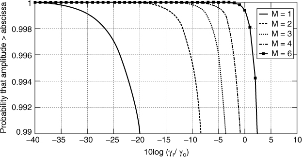
The cumulative density function of γR is given by [38]:
Similarly, Equation (6.48) can be plotted to indicate the gain of the additional branches as shown in Figure 6.51.
Figure 6.51 Cumulative distribution graph of CNR of MRC diversity.
6.9.1.3 Equal-Gain Combining
In this method all of the received signals are equally weighted. This gives an output signal with an envelope similar to MRC where in Equation (6.44) ak = 1 is substituted to give:
6.49 ![]()
This gives an output SNR and is therefore:
6.50 ![]()
Since from Equation (6.45):
![]()
the mean value of the output SNR can be shown to be [38]:
Analytically, equal-gain combining is the most difficult to handle because the output envelope is the sum of M Rayleigh distributed variables. For M > 2 the probability density function of γR can be obtained by numerical integration techniques. The curves lie in between the corresponding ones for MRC and selection systems, and in general are only marginally below MRC curves.
6.9.1.4 Improvements from Diversity
Comparing Equations (6.41), (6.47) and (6.51), the improvements from M branch diversity with respect to the single branch in a Rayleigh fading channel is then given as:
Graphs of Equation (6.52) show that MRC is the best and selection diversity is the worst, with the difference between MRC and EGC being always less than 1.05 dB when M is infinite. Maximum improvement is achieved when going from a single branch to dual diversity.
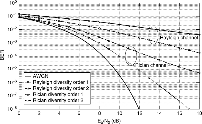
Figure 6.52 illustrates the theoretical enhancement in performance due to MRC diversity gain with the addition of a second branch for two different types of fading channels: Rayleigh fading and Rician fading with k = 10 for PSK modulation. The theoretical error rate in the presence of AWGN is also included for comparison. The BER curves show that at a BER of 1 × 10⁻³ the enhancement is about 1.5 dB for a Rician channel whereas it is significantly greater than 4 dB for a Rayleigh channel.
Figure 6.52 BER for PSK in an AWGN channel, a Rayleigh fading channel and a Rician fading channel with two-branch MRC diversity and without diversity.
6.9.2 Diversity Gain Prediction of Rayleigh Fading Channels from Measurements in a Reverberation Chamber
As discussed in Section 6.2, measurements in reverberation chambers can be set up for an M × M antenna configuration as illustrated in Figure 6.53 to generate Rayleigh fading statistics for multiple antenna configurations including MISO, SIMO and MIMO channels to assess both diversity gains and MIMO capacity.
Figure 6.53 M port vector network analyzer (VNA) in conjunction with an M × M antenna configuration for the estimation of diversity gain.
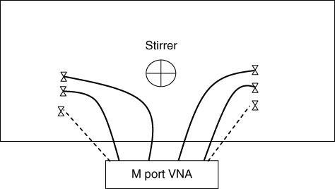
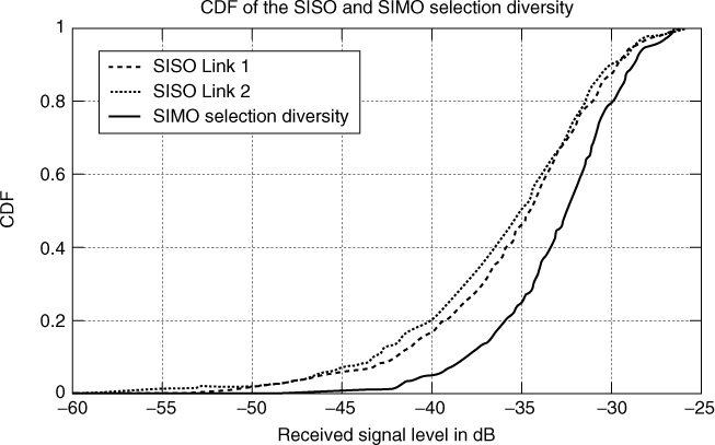
Figure 6.54 gives an example of the apparent diversity gain for a 1 × 2 SIMO configuration for when the signal with the higher SNR is selected in contrast to the single input–single output (SISO) received signal strength. The figure shows that the median diversity gain is 2–2.5 dB over the single branch reception. As in the SISO case, the measurements can be used in a channel simulator in the ‘playback’ scenario.
Figure 6.54 Selection diversity gain estimated from measurements in a reverberation chamber [21].
References
1. Matthias, P., Cheng-Xiang, W. and Hogstad, B.O. (2009) Two new sum-of-sinusoids-based methods for the efficient generation of multiple uncorrelated rayleigh fading waveforms. IEEE Trans. Wirel. Commun., 8 (6), 3122–3131.
2. Gaston, A., Chriss, H.W. and Walker, H.E. (1973) A multi path fading simulator for mobile radio. IEEE Trans. Veh. Technol., 22 (4), 241–244.
3. Golomb, S.W. (1967) Shift Register Sequences, Holden-Day, San Francisco, CA.
4. Hamilton, W.A. and Bodtmann, W.F. (1983) A hybrid multichannel hardware simulator for frequency-selective mobile radio paths. IEEE Trans. Commun., 31 (3), 370–377.
5. Caples, E.L., Massad, K.E. and Minor, T.R. (1980) A UHF channel simulator for digital mobile radio. IEEE Trans. Veh. Technol., 29 (2), 281–289.
6. Jakes, W.C. (1994) Microwave Mobile Communications, IEEE Press, New York.
7. Chen, X.F. and Chung, K.S. (1996) Generation of noise sources for a digital frequency selective fading simulator. International symposium on signal processing and its application, ISSPA, Gold Coast, Australia, August 1996.
8. Lee, Y. and Huang, X. (2002) The simulation of independent Rayleigh faders. IEEE Trans. Commun., 50, 1503–1512.
9. Pätzold, M. (2002) Mobile Fading Channels, 2nd edn, John Wiley & Sons, Ltd, West Sussex.
10. Cavers, J.K. (2002) Mobile Channel Characteristics, Klumer Academic Publisher.
11. Eduardo, C. and Cyril, L. (1990) A simple digital fading simulator for mobile radio. IEEE Trans. Veh. Technol., 39 , 205–212.
12. Chen, X.F. and Chung, K.S. (1996) Generation of noise sources for a digital frequency selective fading simulator. International symposium on signal processing and its application, ISSPA, Gold Coast, Australia, August 1996.
13. Pätzold, M., Garcia, R. and Laue, F. (2000) Design of high speed simulation models for mobile fading channels by using table look-up techniques. IEEE Trans. Veh. Technol., 49 (4), 1178–1190.
14. Rice, S.O. (1944) Mathematical analysis of random noise. Bell Syst. Tech. J., 23 , 282–332.
15. Rice, S.O. (1945) Mathematical analysis of random noise. Bell Syst. Tech. J., 24 , 46–156.
16. Clarke, R.H. (1968) A statistical theory of mobile radio reception. Bell Syst. Tech. J., 47 , 957–1000.
17. Hanzo, L., Webb, W. and Keller, T. (2000) Single and Multi-Carrier Quadrature Amplitude Modulation, John Wiley & Sons, Ltd and IEEE Press,West Sussex.
18. Smith, J.I. (1975) A computer generated multipath simulator for mobile radio. IEEE Trans. Veh. Technol., 24 (3), 39–40.
19. Rappaport, T.S. (1996) Wireless Communications, Principles and Practice, Prentice Hall.
20. Young, J.D. and Beaulieu, N.C. (2000) The generation of correlated Rayleigh random variates by discrete Fourier transform. IEEE Trans. Commun., 48 (7), 1114–1127.
21. Nasr, K.M., Salous, S. and Raimondo, X. (2010) Measurements of the diversity gain of UWB arrays in reverberation and indoor environments, COST 2100 TD(10)12051.
22. Turin, G.L., Clapp, F.D., Johnston, T.L. et al. (1972) A statistical model of urban multi path propagation. IEEE Trans. Veh. Technol., 21 , 1–9.
23. Hashemi, H. (1979) Simulation of urban radio propagation channel. IEEE Trans. Veh. Technol., 28 (3), 213–225.
24. Briso-Rodriguez, C. and Alonso-Montes, J.I. (2001) Multipath hardware and software mobile channel simulator. IEEE VTC 2001, Vol. 4, pp. 3060–3063.
25. Davenport, W.B. and Root, W.L. (1958) An Introduction to the Theory of Random Signals and Noise, McGraw-Hill, New York.
26. Tranter, H.W., Shanmugan, K.S., Rappaport, T.S. and Kosbar, K.L. (2003) Principles of Communication System Simulation with Wireless Applications, Prentice Hall Communications Engineering and Technologies Series, Prentice Hall.
27. Khokhar, K. and Salous, S. (2008) Frequency domain simulator for mobile radio channels and for IEEE 802.16-2004 Standard using measured channels. IET Commun., 2 (7), 869–877. DOI: 10.1049/iet-com:20070385.
28. Khokhar, K. (2006) Design and development of mobile channel simulators using digital signal processing techniques, PhD Thesis submitted to Durham University.
29. Cavers, J.K. (1995) Mobile Channel Characterisation, Kluwer Academic Publisher, Norwood, MA.
30. North, D.O. (1943) An analysis of the factors which determine signal/noise discrimination in pulsed carrier systems. Report PTR-6C, RCA Laboratories, Princeton, NJ.
31. Proakis, J.G. (1995) Digital Communications, 3rd edn, McGraw-Hill.
32. Glover, I. and Grant, P. (1997) Digital Communications, Prentice Hall, Europe.
33. Haykin, S. (2001) Communication Systems, John Wiley & Sons, Inc..
34. Siemons, J.J.J. (2000) Measurement based indoor radio channel model. National Laboratory Report 2000/815.
35. Price, R. and Green Jr, P.E. (1958) A communications technique for multipath channels. Proc. IRE, 46 (3), 555–570.
36. Haykin, S. and Moher, M. (2005) Modern Wireless Communications, Pearson Prentice Hall, Pearson Education, Inc., Upper Saddle River, NJ.
37. Brennan, D.G. (1959) Linear diversity combining techniques. Proc. IRE, 47 , 1057–1102.
38. Parsons, J.D. (2000) The Mobile Radio Propagation Channel, John Wiley & Sons, Inc..