
9
Channel Estimation and Equalization
As we discussed in Chapter 3, a wireless channel is no longer a black box. Wireless communication systems can obtain Channel State Information (CSI) such a fading effect and power delay. The mathematical models of the wireless channels enable us to understand how a received signal is affected by specific environments. Channel estimation is used to obtain CSI and has become a critical part of wireless communication systems. Many communication techniques use this information and improve system performances. Especially, the performance of equalizers and MIMO techniques depends on accuracy of channel estimation.
9.1 Channel Estimation
Channel estimation is simply defined as characterizing a mathematically modeled channel. The mathematical channel model is characterized by long-term CSI (or statistical CSI) and short-term CSI (or instantaneous CSI). Long-term CSI simply means statistical information such as channel statistical distribution and average channel gain. Short-term CSI simply means channel impulse response. Channel estimation algorithms typically find channel impulse response by time domain channel estimation (before DFT processing in OFDM systems) or channel frequency response by frequency domain channel estimation (after DFT processing in OFDM systems). While short-term CSI can be accurately estimated in a slow fading channel, it is difficult to obtain accurate short-term CSI in a fast fading channel. Thus, an adaptive channel estimation algorithm is used for a rapidly time varying channel. An adaptive channel estimation algorithm changes its parameters according to time varying environments. Figure 9.1 illustrates general channel estimation. The design criteria of channel estimators are to minimize a Mean Squared Error (MSE) and computational complexity.

Figure 9.1 General channel estimation
The channel knowledge by channel estimation is very useful to mitigate channel impairments. An equalizer uses this knowledge and reduces inter-symbol interferences. A correlator of a rake receiver uses this knowledge and makes successful despreading. Especially, the capacity of MIMO systems depends on CSI in both a transmitter and a receiver.
Channel estimation can be classified into pilot-assisted channel estimation, blind channel estimation, and Decision-Directed Channel Estimation (DDCE). Pilot-assisted channel estimation is the most popular method that a transmitter sends a known signal, where pilot means the reference signal used by both a transmitter and a receiver. It can be applied to any wireless communication systems and its computational complexity is very low. However, the main disadvantage is the reduction of transmission rate because non-data symbols (pilots) are inserted. Thus, one design challenge of pilot-assisted channel estimation is to minimize the number of pilots and estimate the channel accurately. A pilot assignment method can be mainly classified into block type and comb type as we discussed in Chapter 5. A block-type pilot assignment method is suitable for a slow fading channel because the channel varies slowly over a number of OFDM symbols. On the other hands, a comb-type pilot assignment method is suitable for a fast fading channel because pilots are uniformly distributed over a number of OFDM symbols. Interpolation in frequency domain is required to find a channel response of non-pilot (data) symbols and it is more sensitive to frequency selective channel. Blind channel estimation does not require non-data symbols (pilots) and uses inherent information in the received symbols. Although blind channel estimation does not waist a bandwidth, its computational complexity and latency are significantly higher than pilot-assisted channel estimation. For example, about 100 symbols are required to obtain 1 channel coefficient. Thus, blind channel estimation is rarely used in practical wireless communication systems. DDCE uses both pilot symbols and detected data symbols. It updates the values of channel estimation. Thus, DDCE has a better performance than pilot-assisted channel estimation. Figure 9.2 illustrates simple DDCE structure.

Figure 9.2 Decision-directed channel estimation
The estimated symbol Ŝn in frequency domain is obtained by the previous estimated channel transfer function ![]() and the received symbol Rn in the equalizer (zero-forcing (ZF) algorithm is assumed) as follows:
and the received symbol Rn in the equalizer (zero-forcing (ZF) algorithm is assumed) as follows:

This estimated symbol is demodulated to ![]() . The channel transfer function is updated by this demodulated symbol
. The channel transfer function is updated by this demodulated symbol ![]() and the previous channel transfer function
and the previous channel transfer function ![]() as follows:
as follows:

and
where α is the update factor depending on the quality of the decision symbol. Since DDCE uses both pilot symbols and detected data symbols, fewer pilot symbols are required than pilot-assisted channel estimation.
In this chapter, we focus on pilot-assisted channel estimation in OFDM systems. There are two main design issues for channel estimation in OFDM systems. The first one is pilot design and the second one is channel estimator design with both low complexity and accuracy. The first design issue can be described as where pilot symbols are allocated and how many pilot symbols are used in time and frequency domain. Each question depends on pilot patterns, interval between pilot symbols, and redundancies of OFDM systems. We should select a suitable pilot design pattern among block type, comb type, and lattice type according to system requirements. Pilot symbol spacing is decided by (5.67) and (5.68). If a short pilot interval is designed, channel estimation can be accurate at frequency selective channel and time-varying channel but spectral efficiency would be low due to redundancy increase. The pilot design was already discussed in Chapter 7 and LS and MMSE channel estimation was introduced in Chapter 5. Thus, we design a channel estimator and equalizer for SISO/MIMO-OFDM systems in this chapter.
Channel estimation is carried out for OFDM systems. First of all, we consider a simple signal model as follows:
where Y ![]() is a received OFDM symbol vector,
is a received OFDM symbol vector, ![]() is a diagonal transmitted OFDM symbol matrix including transmitted data, pilots, and null signals,
is a diagonal transmitted OFDM symbol matrix including transmitted data, pilots, and null signals, ![]() is a channel frequency response vector we should estimate, and
is a channel frequency response vector we should estimate, and ![]() is a white Gaussian noise vector. The channel frequency response H can be expressed as the channel impulse response
is a white Gaussian noise vector. The channel frequency response H can be expressed as the channel impulse response ![]() and (9.4) is rewritten as follows:
and (9.4) is rewritten as follows:
where ![]() is the channel impulse response and
is the channel impulse response and ![]() is the DFT matrix as follows:
is the DFT matrix as follows:
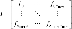
where NIDFT is the IDFT size. Pilot-assisted channel estimation uses a part of subcarriers as a pilot. An interpolation technique should be performed to obtain a channel estimation value at each data subcarrier. In order to simplify the system model and reduce the complexity of the channel estimator, we consider two assumptions [1]. The first assumption is that we consider a finite length impulse response and deal with only significant channel tap. That is, when the channel impulse response h has the maximum delay at tap [0, L−1], the first L columns of F are considered. The second assumption is that only rows of F corresponding to the position of pilots are considered for the transmitted matrix X because the pilots are distributed in the OFDM symbol. Thus, we have the following equation:
where ![]() ,
, ![]() , and
, and ![]() are the received pilot symbol matrix, channel impulse response matrix, and white Gaussian noise matrix associated with the transmitted pilot symbol, respectively. Xp is the diagonal pilot symbol matrix and Tp is the DFT matrix corresponding to the transmitted pilot symbol as follows:
are the received pilot symbol matrix, channel impulse response matrix, and white Gaussian noise matrix associated with the transmitted pilot symbol, respectively. Xp is the diagonal pilot symbol matrix and Tp is the DFT matrix corresponding to the transmitted pilot symbol as follows:

and

where NDFT is the DFT size, Np is the number of pilot subcarriers, and ip is the pilot index. The channel impulse response matrix is reduced to an L × L matrix. This result significantly affects LS and MMSE estimation.
The block-type pilot-assisted channel estimation method can be performed under the assumption of a slow fading channel. The pilots are inserted in all subcarriers. Thus, interpolation is not needed. However, the comb-type pilot-assisted channel estimation method can be developed under the assumption of channel change in OFDM symbol sequences. Thus, interpolation is needed to estimate a whole subcarrier. As we discussed in Chapter 5, the receiver estimates the channel condition based on LS and MMSE algorithms. When considering the comb-type pilot channel estimation method, the pilots are uniformly inserted and the kth subcarrier in the OFDM symbol can be expressed as follows:

where m and D are a pilot subcarrier (0 ≤ m ≤ Np−1) and NDFT/Np (0 ≤ d < D), respectively. LS channel estimation determining the channel frequency response is calculated as follows:

This is estimated for only pilot subcarriers. Thus, channel estimation results should be interpolated over a whole subcarrier including data subcarriers. One easiest way is to connect two pilots with straight lines. We call it piecewise constant interpolation (or nearest neighbor interpolation). It allocates same pilot values to near data subcarriers. Another simple interpolation is linear interpolation. It allocates the values on the straight line between two pilots. Linear interpolation has better performance than piecewise constant interpolation [2]. When we have two pilots (e.g., (H(a), a) and (H(b), b)), the interpolant (H(c), c) satisfies the following equation:
and the interpolant at the data subcarrier is represented as follows:
Thus, we express channel estimation values (He(k)) at data subcarriers as follows [3]:
where k is the data subcarrier (mD ≤ k < (m + 1)D). Linear interpolation is simple but does not produce accurate interpolants. Thus, polynomial interpolation is widely used. It is the generalized form of linear interpolation. The order of polynomial interpolation is defined as the number of given data (or pilots) minus one. The first-order interpolation (e.g., when we consider only two pilots) is linear interpolation. Basically, a high-order interpolation generates wild oscillations. The practical limitation is the fifth-order interpolation. Thus, the second-order polynomial interpolation is good choice according to performance and complexity. It shows us better performance than linear interpolation. The channel estimation values are decided by linear combination of the weighted pilot values. We express channel estimation values (He(k)) at data subcarriers as follows [3]:
where

Another practical interpolation is low-pass interpolation (or upsampling). It has simple two-step process. The first step is to insert zeros into the channel estimation position (data subcarriers) and the second step is to put the sequence into low-pass filter (LPF; FIR filter). Figure 9.3 illustrates one example of low-pass interpolation by a factor of 2. As we can observe, the inserted zeros by upsampling increase the data rate but there is no effect to sample distribution. After passing through LPF, the inserted zeros are replaced by interpolants.

Figure 9.3 Example of low-pass interpolation
LS channel estimation is simple but the performance is not good. In block-type pilot assignment, the MMSE estimator has about 10–15 dB better performance than the LS estimator for the same MSE value [1]. The MMSE estimator calculates the channel impulse response (CIR) which minimizes the means squared error between the exact CIRs and the estimated CIRs. One disadvantage of MMSE estimators is a high complexity. It increases exponentially according to observation samples. Thus, a linear MMSE (LMMSE) estimator is widely used in the OFDM system. In Ref. [4], low rank approximation based on the DFT is proposed and the complexity is reduced by singular value decomposition. The LMMSE estimator uses the frequency correlation of the channel. It can be calculated as follows [1]:
where ![]() is the cross-correlation matrix between all subcarriers and pilots,
is the cross-correlation matrix between all subcarriers and pilots, ![]() is the auto-correlation matrix between pilots, and
is the auto-correlation matrix between pilots, and ![]() is the noise variance. The correlation matrices are defined as follows:
is the noise variance. The correlation matrices are defined as follows:
As we can observe from (9.17), the LMMSE calculation is very complex. We need simpler equation. If the LMMSE equation does not depend on the transmitted symbols, the calculation can be significantly reduced. Thus, the simplified LMMSE estimator is expressed as follows [4]:
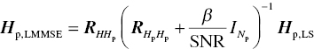
where

and SNR is average signal to noise radio at subcarriers. β is constant depending on signal constellation. For example, ![]() for QPSK and
for QPSK and ![]() for 16 QAM [5]. The simplification comes from SNR estimation simplification. Thus, this equation would not provide accurate channel estimation when it is difficult to obtain SNR levels in the whole OFDM subcarrier [6]. When a block-type pilot assignment method is considered, the LMMSE estimator is rewritten as follows:
for 16 QAM [5]. The simplification comes from SNR estimation simplification. Thus, this equation would not provide accurate channel estimation when it is difficult to obtain SNR levels in the whole OFDM subcarrier [6]. When a block-type pilot assignment method is considered, the LMMSE estimator is rewritten as follows:

In a practical system, the channel autocorrelation and SNR can be set to known factors at the receiver in advance. The channel autocorrelation calculation and SNR estimation affect the performance. The channel correlation matrices are derived in Ref. [4]. Thus, the term W is calculated only once. Equation 9.22 can be simplified in order to reduce multiplications. The correlation term can be decomposed by singular value decomposition (SVD) as follows:
where U and Λ are a unitary matrix and a diagonal matrix containing the singular values, ![]() , respectively. When m rank approximation is applied, (9.22) is rewritten as follows:
, respectively. When m rank approximation is applied, (9.22) is rewritten as follows:
where Δm is a diagonal matrix containing the following entries:
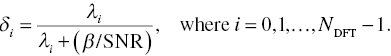
(9.24) is much simpler than (9.22) because the number of singular value m is much smaller than NDFT.
When a receiver has additional statistical information such as channel autocorrelation matrix and average SNR, the LMMSE estimator shows us good performance. Especially, in a low SNR scenario, it brings much better performance than the LS estimator. On the other hand, additional statistical information produces additional latency and complexity.
9.2 Channel Estimation for MIMO–OFDM System
MIMO–OFDM systems send symbols via multiple transmit antennas and receive the superposition of the symbols from multiple receive antennas. The superposed symbols should be extracted and the inter-antenna interference should be eliminated. Thus, channel estimation for multiple antenna systems cannot be simply transformed from single antenna systems. Channel estimation for MIMO–OFDM systems is more complicated than single antenna systems but the basic principle is similar to the single antenna systems.
One simple pilot assignment for MIMO–OFDM systems is the grid-type pilot assignment in both frequency domain and time domain as shown in Figure 9.11.
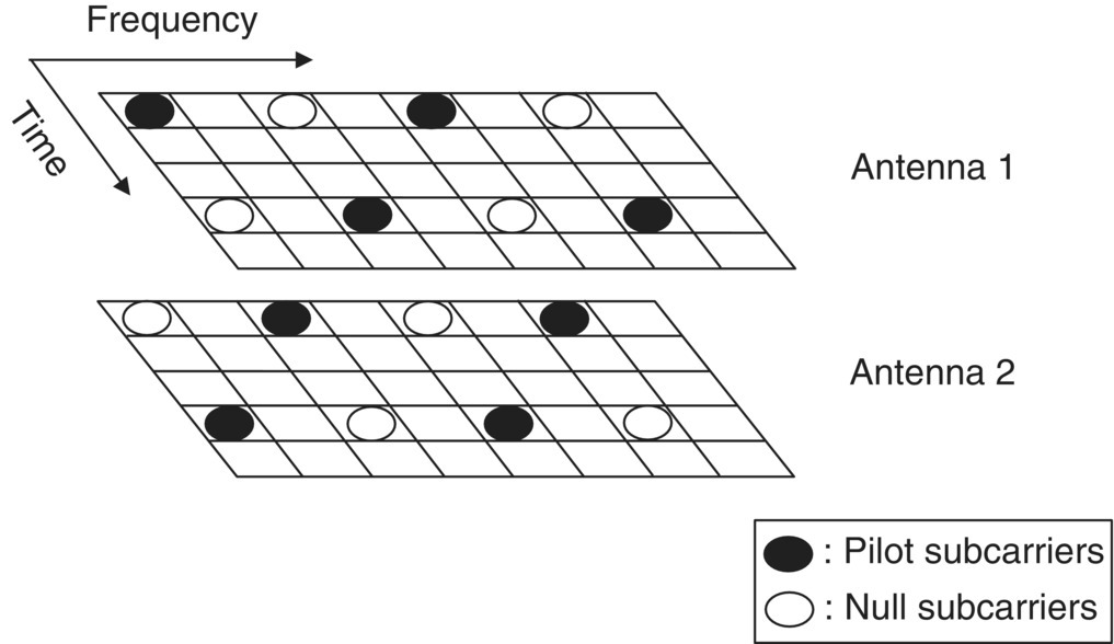
Figure 9.11 Pilots assignment for MIMO OFDM system
One transmit antenna sends its pilot at a given subcarrier while the other antenna remains silent (null subcarrier) [7]. This pilot assignment method protects each pilot from signals of the other antennas. The inter-antenna interference is easily eliminated. However, the disadvantage is to reduce spectral efficiency due to null subcarriers. In addition, the null subcarriers increase the Peak to Average Power Ratio (PAPR) [8]. It is essential that a transmitter has a power amplifier which provides a suitable power for transmission. The power amplifier is very sensitive to operational area which requires a linear area. A high PAPR causes a nonlinear operation problem so that it causes signal distortion. Therefore, the PAPR should be well managed in the OFDM system. In order to estimate the MIMO channel for a space time block code, the channel can be assumed stationary during L OFDM symbols transmission. Thus, the MIMO channel matrix is represented as follows:

and
where Nt, Nr, and ck are the total transmit antennas, the total receive antennas, and the kth subcarrier, respectively. The pilot signals at subcarrier ck are transmitted at the ith transmit antenna as follows:
and the L × L pilot matrix is represented as follows:
The received pilot signals at the jth received antenna are represented as follows:
and the corresponding MIMO channel is represented as follows:
Thus, the received signal vector at the jth receive antenna is expressed as follows:
where ![]() is a Gaussian noise vector. If the pilot signal matrix
is a Gaussian noise vector. If the pilot signal matrix ![]() is a unitary matrix, the matrix
is a unitary matrix, the matrix ![]() is invertible. The channel frequency response is obtained using LS estimation as follows:
is invertible. The channel frequency response is obtained using LS estimation as follows:
The MIMO channel estimation strategy does not fit in the non-stationary channel. Thus, the superposed pilot based channel estimation strategy and the optimal pilot assignment method are investigated in Ref. [9]. They do not use null subcarriers and a prior information. It provides higher spectral efficiency than when null subcarriers are employed. The disadvantage is that the pilot design condition is tricky. Thus, in practical systems such as WiMAX and LTE, the grid-type pilot assignment method using null subcarriers is adopted as shown in Figure 9.11.
9.3 Equalization
As we briefly discussed in Chapter 5, the purpose of equalizers is to find the inverse function of the channel response and eliminate an Inter-Symbol Interference (ISI) caused by the dispersive nature of the channel. The equalizers can be classified into several different ways. One criterion of the classifications is whether they are adaptive equalizers or non-adaptive equalizers. Adaptive equalizers are used when the channel is time varying. The filter coefficients of the equalizers are changed according to time-varying channel. Non-adaptive equalizers are used for timing invariant channels and designed by the inverse function of the channel response. Another criterion of the classifications is whether they are linear or non-linear equalizers. The linear equalizers are based on the tap delayed equalization. They do not have a feedback path. The output is linear combination of the inputs. On the other hands, the non-linear equalizers have a feedback path and are used when a receiver copes with a large ISI. In OFDM systems, it can be classified in Time Domain eQualization (TEQ) or Frequency Domain eQualization (FEQ). The TEQ deals with the time domain symbol before carrying out DFT/FFT of the receiver. The FEQ is simple and less complex than the TEQ. Once channel estimation is finished, the FEQ is carried out in order to compensate for signal distortion at each subcarrier. A one-tap FEQ is widely used in the OFDM system because a frequency selective channel is regarded as a flat fading channel at each subcarrier. However, when we consider a fast fading channel, the channel state is changed in one OFDM symbol period and an Inter-Carrier Interference (ICI) occurs. Thus, the OFDM receiver should remove the ICI. FEQ was invented in 1970s but was not widely recognized. After multicarrier systems appeared, FEQ was recognized because it well matches with OFDM systems and provides us with good performance in a frequency selective fading channel. Another important equalizer is the Turbo equalizer which is inspired from Turbo codes [10]. Basically, the received signals suffer from an ISI and noise. An equalizer suppresses the ISI and an error control code corrects or detects a corrupted codeword bit. Conventional approach is to suppress the interference from the received signals and then decode the received codewords. However, the Turbo equalizer performs equalization and decoding together. In other words, it estimates, equalizes, decodes, and re-encodes, iteratively. During the iteration, accurate estimation results can be obtained and simultaneously it provides us with more precise equalization.
In a time-invariant channel (for example, when the channel impulse response is constant in one OFDM symbol period), the received signal Yk, i is expressed as follows:
where Hk, i, Xk, i, and Nk,i are the channel frequency response, the transmitted signal, and the Gaussian noise at the kth subcarrier and the ith OFDM symbol, respectively. The one tap FEQ is carried out as follows:
where Gk,i is the equalizer coefficient. The ZF equalizer simply applies the inverse of the channel frequency response to the received OFDM symbol. It changes a frequency selective fading at a whole OFDM symbol to a flat fading at one subcarrier. The ZF equalizer coefficient is expressed as follows:
where Ĥk,i is the channel response estimation. Figure 9.12 illustrates the ZF equalizer.

Figure 9.12 Zero forcing equalizer
Since this approach ignores the Gaussian noise of (9.34), it may amplify a noise in the subcarriers. In particular, the equalizer performance is poor at a low SNR. The MMSE equalizer takes the Gaussian noise into account and achieves a better performance. It tries to minimize the variance of the difference (or the mean square error) between the output of the equalizer and the transmitted symbol. It is expressed as follows [11]:

Figure 9.13 illustrates the MMSE equalizer.

Figure 9.13 MMSE equalizer
Adaptive equalizers compare the output of the equalizer with the pilot signals and then calculate an error signal. Thus, the equalizer coefficients are adjusted by the error signal ![]() as follows:
as follows:
where ![]() is the weight factor.
is the weight factor.
9.4 Hardware Implementation of Channel Estimation and Equalizer for OFDM System
The channel estimator and the equalizer are designed according to the system requirements such as pilot assignment, antenna array, system complexity, latency, and power. Especially, the latency is strict design parameter because channel estimation and interpolation must be finished and the equalizer must be ready when the data OFDM symbol is arrived at the receiver. In this section, we briefly investigate a simple LS estimator and ZF equalizer design in the OFDM system with the block-type pilot assignment and single antenna. Figure 9.14 illustrates a simple LS estimator and ZF equalizer block diagram. When the received pilot OFDM symbol Yk,i is arrived, the LS estimator calculate (9.11) with the stored pilot OFDM symbol. In this calculation, we deal with a complex number and division. Thus, Euler’s theorem ![]() can be used for simple calculation. The conversion can be obtained by the CORDIC algorithm. This conversion is also useful in the inverse of the channel response block. The ZF equalizer collects the data OFDM symbol and the inverse of the channel response and then calculates simple multiplications. Sometime, a phase offset is compensated in this process. Once the pilot subcarriers are detected, they are compared with the stored pilot subcarriers and the phase difference is calculated. In the ZF equalizer, it is compensated.
can be used for simple calculation. The conversion can be obtained by the CORDIC algorithm. This conversion is also useful in the inverse of the channel response block. The ZF equalizer collects the data OFDM symbol and the inverse of the channel response and then calculates simple multiplications. Sometime, a phase offset is compensated in this process. Once the pilot subcarriers are detected, they are compared with the stored pilot subcarriers and the phase difference is calculated. In the ZF equalizer, it is compensated.

Figure 9.14 LS estimator and ZF equalizer
9.5 Problems
- 9.1. Compare the performances of time domain channel estimation and frequency domain channel estimation for an OFDM system.
- 9.2. Compare the MSEs of pilot-assisted channel estimation, blind channel estimation, and DDCE.
- 9.3. Describe the pilot assignment of a 4 × 4 MIMO OFDM system in the LTE standard.
- 9.4. Compare the Lagrangian interpolation with the Newton interpolation.
- 9.5. Define the error that can occur in polynomial interpolation and describe the method to minimize the error.
- 9.6. Consider the following system model:
 where y(k), H, x(k), and z(k) are the received signal vector, channel matrix, transmitted signal vector, and white Gaussian noise vector, respectively. Find the optimal precoding matrix W such that
  .
. - 9.7. Channel estimation errors result in system performance degradation. Define the channel estimation error in an OFDM system and describe its effect to system performance.
References
- [1] J. Beek, O. Edfors, M. Sandell, S. Wilson, and P. Börjesson, “On Channel Estimation in OFDM Systems,” Proceedings of IEEE the 45th Vehicular Technology Conference (VTC’95), Chicago, IL, vol. 2, pp. 815–819, July 25–28, 1995.
- [2] L. J. Cimini, “Analysis and Simulation of a Digital Mobile Channel Using Orthogonal Frequency Division Multiplexing,” IEEE Transactions on Communications, vol. 33, no. 7, pp. 665–675, 1985.
- [3] M. Hsieh and C. Wei, “Channel Estimation for OFDM Systems Based on Comb-Type Pilot Arrangement in Frequency Selective Fading Channels,” IEEE Transactions on Consumer Electronics, vol. 44, no. 1, p. 217, 1998.
- [4] O. Edfors, M. Sandell, J. J. van de Beek, S. K. Wilson, and P. O. Borjesson, “OFDM Channel Estimation by Singular Value Decomposition,” IEEE Transactions on Communications, vol. 46, no. 7, pp. 931–939, 1998.
- [5] A. Khlifi and R. Bouallegue, “Performance Analysis of LS and LMMSE Channel Estimation Techniques for LTE Downlink Systems,” International Journal of Wireless and Mobile Network, vol. 3, no. 5, pp. 141–149, 2011.
- [6] M. Rim, J. Ahn, and Y. Kim, “Decision-Directed Channel Estimation for M-QAM Modulated OFDM Systems,” Proceedings of IEEE the 55th Vehicular Technology Conference (VTC spring ’02), vol. 4, pp. 1742–1746, Birmingham, AL, USA, May 6–9, 2002.
- [7] W. G. Jeon, K. H. Paik, and Y. S. Cho, “An Efficient Channel Estimation Technique for OFDM systems with Transmitter Diversity,” Proceedings of IEEE the 11th Personal, Indoor and Mobile Radio Communication Conference (PIMRC 2000), vol. 2, pp. 1246–1250, London, UK, September 18–21, 2000.
- [8] A. Dowler and A. Nix, “Performance Evaluation of Channel Estimation Techniques in a Multiple Antenna OFDM System,” Proceedings of IEEE Vehicular Technology Conference (VTC’03), vol. 2, pp. 1214–1218, Orlando, FL, USA, October 6–9, 2003.
- [9] Y. Li, “Simplified Channel Estimation for OFDM Systems with Multiple Transmit Antennas,” IEEE Transactions on Wireless Communications, vol. 1, no. 1, pp. 67–75, 2002.
- [10] C. Douillard, M. Jézéquel, and C. Berrou, “Iterative Correction of Intersymbol-Interference: Turbo-Equalization,” European Transactions on Telecommunications, vol. 6, no. 5, pp. 507–511, 1995.
- [11] T. Chiueh and P. Tsai, OFDM Baseband Receiver Design for Wireless Communications, John Wiley & Sons, Inc., Hoboken, NJ, 2007.