Search in book...
Toggle Font Controls
Create new playlist

Name your new playlist

Playlist description (optional)
Sign In

Email address

Password

Forgot Password?

or

Continue with Facebook

Continue with Google
Sign Up

Full Name

Email address

Confirm Email Address

Password

or

Continue with Facebook

Continue with Google

CHAPTER 1
A Primer on Banking, Finance and Financial Instruments

“People still crave explanations even when there is no underlying understanding about what's going on…erratic stock market movements always find a ready explanation in the next day's financial columns: a price rise is attributed to sentiment that ‘pessimism about interest rate increases was exaggerated,’ or to the view that ‘company X had been oversold.’ Of course these explanations are always a posteriori: commentators could offer an equally ready explanation if a stock price had moved the other way.”

—Professor Martin Rees, Our Cosmic Habitat, Phoenix 2003, page 101

This chapter is reference material for newcomers to the market, junior bankers and finance students, or for those that require a refresher course on the core subject matter. The purpose of this primer is to introduce all the essential basics of banking, which is necessary if one is to gain a strategic overview of what banks do, what risk exposures they face and how to manage them properly. We begin with the concept of banking, and follow this with a description of bank cash flows, calculation of return, the risks faced in banking, and organisation and strategy.

Banking is a subset of “finance”. The principles of finance underlay the principles of banking. It would be difficult to become conversant with the principles of banking, and thus be in a position to manage a bank efficiently and effectively to the benefit of all stakeholders, unless one was also familiar with the principles of finance. That said, it is not uncommon to encounter senior executives and non‐executive directors on bank Boards who are perhaps not as au fait with basic principles as they should be. Hence, these basic principles are introduced here and remain the theme of Part I of this book.

AN INTRODUCTION TO BANKING

This extract from Bank Asset and Liability Management (2007)

Introduction

As Sir Arthur Conan Doyle would have put it, so elementary a form of literature as the textbook on financial economics hardly deserves the dignity of a preface. It is possible, though, to bring some instant clarity to the purpose of such a book if we open with a few words here.

The traditional view of a bank is that of a financial institution that is in the business of taking deposits and advancing loans, and which makes its money from the difference in interest rate paid and received on these two products. While this quaint image would have been true a few hundred years ago, it is decidedly incomplete today. The modern banking institution is a complex beast, which in many cases operates in a wide range of products and services and across international markets. Banks are the cornerstone of the global economy, and at the highest level the banking sector influences, and is influenced by, macroeconomic trends such as GDP growth, central bank base interest rates, equity and debt capital markets activity, and the supply and demand for investments and credit.

However, notwithstanding our first statement that banks now engage in many complex activities outside traditional borrowing and lending, we must remember that at the core of all capital markets activity lies the need to bring together the suppliers of capital with the borrowers of capital. This was the original business logic behind the very first banks, so in that respect very little has changed! There is much other activity surrounding this basic function in the markets, but this need is paramount. Hence a key ingredient in bank strategy is the management of its assets and liabilities. It is this that is the subject of this book: Asset and Liability Management (ALM). These days there are a large number of instruments, in cash and derivative form, that make up a bank's assets and liabilities. No matter. For the ALM desk in a bank, the cash assets and liabilities are king and must be managed prudently. That there is more to this than may meet the eye is apparent immediately from the thickness of this book!

Let us set the scene further with some discussion on banks.

Introduction

Banking operations encompass a wide range of activities, all of which contribute to the asset and liability profile of a bank. Table P.1 shows selected banking activities, and the type of risk exposure they represent. The terms used in the table, such as “market risk”, are explained elsewhere in this book. In Chapter 2 we discuss elementary aspects of financial analysis, using key financial ratios, that are used to examine the profitability and asset quality of a bank. We also discuss bank regulation and the concept of bank capital.

Table P.1 Selected banking activities and services

Service or function	Revenue generated	Risk
Lending
– Retail	Interest income, fees	Credit, Market
– Commercial	Interest income, fees	Credit, Market
– Mortgage	Interest income, fees	Credit, Market
– Syndicated	Interest income, fees	Credit, Market
Credit cards	Interest income, fees	Credit, Operational
Project finance	Interest income, fees	Credit
Trade finance	Interest income, fees	Credit, Operational
Cash management
– Processing	Fees	Operational
– Payments	Fees	Credit, Operational
Custodian	Fees	Credit, Operational
Private banking	Commission income, interest income, fees	Operational
Asset management	Fees, performance payments	Credit, Market, Operational
Capital markets
– Investment banking	Fees	Credit, Market
– Corporate finance	Fees	Credit, Market
– Equities	Trading income, fees	Credit, Market
– Bonds	Trading income, interest income, fees	Credit, Market
– Foreign exchange	Trading income, fees	Credit, Market
– Derivatives	Trading income, interest income, fees	Credit, Market

Before considering the concept of ALM, all readers should be familiar with the way a bank's earnings and performance are reported in its financial statements. A bank's income statement will break down the earnings by type, as we have defined in Table P.1. So we need to be familiar with interest income, trading income and so on. The other side of an income statement is the costs, such as operating expenses and bad loan provisions.

That the universe of banks encompasses many different varieties of beast is evident from the way they earn their money. Traditional banking institutions, perhaps typified by a regional bank in the United States or a building society in the United Kingdom, will generate a much greater share of their revenues through net interest income than trading income, and vice versa for an investment bank such as Lehman International or Merrill Lynch. The latter firms will earn a greater share of their revenues through fees and trading income.

During 2004 a regional European bank reported the following earnings breakdown, as shown in Table P.2.

Table P.2 European regional bank, earnings structure 2004

Source: Author's notes.

Core operating income	% share
Net interest income	62
Fees and commissions	27
Trading income	11

However, this breakdown varies widely across regions and banks, and in fact would be reversed at an investment bank whose core operating activity was market‐making and proprietary trading.

Let us consider now the different types of income stream and costs.

Interest income

Interest income, or net interest income (NII), is the main source of revenue for the majority of banks worldwide. As we saw from Table P.2, it can form upwards of 60% of operating income, and for smaller banks and building societies it reaches 80% or more.

NII is generated from lending activity and interest‐bearing assets, the “net” return is this interest income minus the cost of funding the loans. Funding, which is a cost to the bank, is obtained from a wide variety of sources. For many banks, deposits are a key source of funding, as well as one of the cheapest. They are generally short‐term, though, or available on demand, so they must be supplemented with longer term funding. Other sources of funds include senior debt, in the form of bonds, securitised bonds and money market paper.

NII is sensitive to both credit risk and market risk. Market risk, which we will look at later, is essentially interest‐rate risk for loans and deposits. Interest‐rate risk will be driven by the maturity structure of the loan book, as well as the match (or mismatch) between the maturity of the loans against the maturity of the funding. This is known as the interest‐rate gap.

Fees and commissions

Banks generate fee income as a result of the provision of services to customers. Fee income is very popular with bank senior management because it is less volatile and not susceptible to market risk like trading income or even NII. There is also no credit risk because the fees are often paid up front. There are other benefits as well, such as the opportunity to build up a diversified customer base for this additional range of services, but these are of less concern to a bank ALM desk.

Fee income uses less capital and also carries no market risk, but does carry other risks such as operational risk.

Trading income

Banks generate trading income through trading activity in financial products such as equities (shares), bonds and derivative instruments. This includes acting as a dealer or market‐maker in these products, as well as taking proprietary positions for speculative purposes. Running positions in securities (as opposed to derivatives) in some cases generates interest income, some banks strip this out of the capital gain made when the security is traded to profit, while others include it as part of overall trading income.

Trading income is the most volatile income source for a bank. It also carries relatively high market risk, as well as not inconsiderable credit risk. Many banks, although by no means all, use the Value‐at‐Risk (VaR) methodology to measure the risk arising from trading activity, which gives a statistical measure of expected losses to the trading portfolio under certain selected market scenarios.

Costs

Bank operating costs comprise staff costs, as well as other costs such as premises, information technology and equipment costs. Further significant elements of cost are provisions for loan losses, which are a charge against the loan revenues of the bank. The provision is based on a subjective measure by management of how much of the loan portfolio can be expected to be repaid by the borrower.

Bank Business and Bank Capital

Banking has a long and honourable history. Today it encompasses a wide range of activities, of varying degrees of complexity. Whatever the precise business, the common denominators of all banking activities are those of risk, return and the bringing together of the providers of capital. Return on capital is the focus of banking activity. The coordination of all banking activity could be said to be the focus of asset and liability management (ALM), although some practitioners will give ALM a narrower focus. Either way, we need to be familiar with the wide‐ranging nature of banking business, and the importance of bank capital. This then acts as a guide for what follows.

In this introductory chapter of the first part of the book, we place ALM in context by describing the financial markets and the concept of bank capital. Subsequent chapters look at money market instruments and the basics of bank financial statements. We begin with a look at the business of banking. We then consider the different types of revenue generated by a bank, the concept of the banking book and the trading book, and financial statements. The chapter concludes with an introduction to the money market, the key area of involvement for an ALM desk.

Banking business

We introduced the different aspects of banking business in the Preface. For the largest banks these aspects are widely varying in nature. For our purposes we may group them together in the form shown in Figure 1.1. Put very simply, “retail” or “commercial” banking covers the more traditional lending and trust activities, while “investment” banking covers trading activity and fee‐based income such as stock exchange listing and mergers and acquisition (M&A). The one common objective of all banking activity is return on capital. Depending on the degree of risk it represents, a particular activity will be required to achieve a specified return on the capital it uses. The issue of banking capital is vital to an appreciation of the banking business; entire new business lines (such as securitisation) have been originated in response to a need to generate more efficient use of capital.

As we can see from Figure 1.1, the scope of banking business is vast. The activities range from essentially plain vanilla activity, such as corporate lending, to complex transactions such as securitisation and hybrid products trading. There is a vast literature on all these activities, so we do not need to cover them here. However, it is important to have a basic general knowledge of the basic products, so subsequent chapters will introduce these.

Figure 1.1 Scope of banking activities

ALM is concerned with, among other things, the efficient management of banking capital. It therefore concerns itself with all banking operations, even if the day‐to‐day contact between the ALM desk (or Treasury desk) with other parts of the bank is remote. The ALM desk will be responsible for the treasury and money markets activities of the entire bank. So if we wish, we could draw a box with ALM in it around the whole of Figure 1.1. This is not to say that the ALM function does all these activities; rather, it is just to make clear that all the various activities represent assets and liabilities for the bank, and one central function is responsible for this side of these activities.

For capital management purposes a bank's business is organised into a “banking book” and a “trading book”. We consider them next; first though, a word on bank capital.

Capital

Bank capital is the equity of the bank. It is important as it is the cushion that absorbs any unreserved losses that the bank incurs. By acting as this cushion, it enables the bank to continue operating and thus avoid insolvency or bankruptcy during periods of market correction or economic downturn. When the bank suffers a loss or writes off a loss‐making or otherwise economically untenable activity, the capital is used to absorb the loss. This can be done by eating into reserves, freezing dividend payments or (in more extreme scenarios) a write‐down of equity capital. In the capital structure, the rights of capital creditors, including equity holders, are subordinated to senior creditors and deposit holders.

Banks occupy a vital and pivotal position in any economy, as suppliers of credit and financial liquidity, so bank capital is important. As such, banks are heavily regulated by central monetary authorities, and their capital is subject to regulatory rules governed by the Bank for International Settlements (BIS), based in Basel, Switzerland. For this reason its regulatory capital rules are often called the Basel rules. Under the original Basel rules (“Basel I”) a banking institution was required to hold a minimum capital level of 8% against the assets on its book.¹ Total capital is comprised of:

equity capital;
reserves;
retained earnings;
preference share issue proceeds;
hybrid capital instruments;
subordinated debt.

Capital is split into Tier 1 capital and Tier 2 capital. The first three items above comprise Tier 1 capital while the remaining items are Tier 2 capital.

The quality of the capital in a bank reflects its mix of Tier 1 and 2 capital. Tier 1 or “core capital” is the highest quality capital, as it is not obliged to be repaid, and moreover there is no impact on the bank's reputation if it is not repaid. Tier 2 is considered lower quality as it is not “loss absorbing”; it is repayable and also of shorter‐term than equity capital. Assessing the financial strength and quality of a particular banking institution often requires calculating key capital ratios for the bank and comparing these to market averages and other benchmarks.

Analysts use a number of ratios to assess bank capital strength. Some of the more common ones are shown in Table 1.1.

Table 1.1 Bank analysis ratios for capital strength

Source: Higson (1995)

Ratio	Calculation	Notes
Core capital ratio	Tier 1 capital/Risk‐weighted assets	A key ratio monitored in particular by rating agencies as a measure of high‐quality non‐repayable capital, available to absorb losses incurred by the bank
Tier 1 capital ratio	Eligible Tier 1 capital/Risk‐weighted assets	Another important ratio monitored by investors and rating agencies. Represents the amount of high‐quality, non‐repayable capital available to the bank
Total capital ratio	Total capital/Risk‐weighted assets	Represents total capital available to the bank
Off‐balance sheet risk to total capital	Off‐balance sheet and contingent risk/Total capital	Measure of adequacy of capital against off‐balance sheet risk including derivatives exposure and committed, undrawn credit lines

Banking and trading books

Banks and financial institutions make a distinction between their activities for capital management, including regulatory capital, purposes. Activities are split into the “banking book” and the “trading book”. Put simply, the banking book holds the more traditional banking activities such as commercial banking; for example, loans and deposits. This would cover lending to individuals as well as corporates and other banks, and so will interact with investment banking business.² The trading book records wholesale market transactions, such as market making and proprietary trading in bonds and derivatives. Again speaking simply, the primary difference between the two books is that the over‐riding principle of the banking book is one of “buy and hold”; that is, a long‐term acquisition. Assets may be held on the book for up to 30 years or longer. The trading book is just that, it employs a trading philosophy so that assets may be held for very short terms, less than one day in some cases. The regulatory capital and accounting treatment of each book differs. The primary difference here is that the trading book employs the “mark‐to‐market” approach to record profit and loss (p&l), which is the daily “marking” of an asset to its market value. An increase or decrease in the mark on the previous day's mark is recorded as an unrealised profit or loss on the book: on disposal of the asset, the realised profit or loss is the change in the mark at disposal compared to its mark at purchase.

The banking book

Traditional banking activity such as deposits and loans is recorded in the banking book. Accounting treatment for the banking book follows the accrual concept, which is accruing interest cash flows as they occur. There is no mark‐to‐market. The banking book holds assets for which both corporate and retail counterparties as well as banking counterparties are represented. So it is the type of business activity that dictates whether it is placed in the banking book, not the type of counterparty or which department of the bank is conducting it. Assets and liabilities in the banking book generate interest‐rate and credit risk exposure for the bank. They also create liquidity and term mismatch (“gap”) risks. Liquidity refers to the ease with which an asset can be transformed into cash, as well as to the ease with which funds can be raised in the market. So we see that “liquidity risk” actually refers to two related but separate issues.

All these risks form part of ALM. Interest‐rate risk management is a critical part of Treasury policy and ALM, while credit risk policy will be set and dictated by the credit policy of the bank. Gap risk creates an excess or shortage of cash, which must be managed. This is the cash management part of ALM. There is also a mismatch risk associated with fixed‐rate and floating‐rate interest liabilities. The central role of the financial markets is to enable cash management and interest‐rate management to be undertaken efficiently. ALM of the banking book will centre on interest‐rate risk management and hedging, and liquidity management. Note how there is no “market risk” for the banking book in principle, because there is no marking‐to‐market. However, the interest rate exposure of the book creates an exposure that is subject to market movements in interest rates, so in reality the banking book is indeed exposed to market risk.

Trading book

Wholesale market activity, including market making and proprietary trading, is recorded in the trading book. Assets on the trading book can be expected to have a high turnover, although not necessarily so, and are marked‐to‐market daily. The counterparties to this trading activity can include other banks and financial institutions such as hedge funds, corporates and central banks. Trading book activity generates the same risk exposure as that on the banking book, including market risk, credit risk and liquidity risk. It also creates a need for cash management. Much trading book activity involves derivative instruments, as opposed to “cash” products. Derivatives include futures, swaps and options. These can be equity, interest‐rate, credit, commodity, foreign exchange (FX), weather and other derivatives. Derivatives are known as “off‐balance sheet” instruments because they are recorded off the (cash) balance sheet. Their widespread use and acceptance has greatly improved the efficiency of the risk exposure hedging process, for banks and other institutions alike.

Off‐balance sheet transactions refer to “contingent liabilities”, which are so‐called because they refer to a future exposure contracted now. These are not only derivatives contracts such as interest‐rate swaps or writing an option, but include guarantees such as a credit line to a third‐party customer or a group subsidiary company. These represent a liability for the bank that may be required to be honoured at some future date. In most cases they do not generate cash inflow or outflow at inception, unlike a cash transaction, but represent future exposure. If a credit line is drawn on, it represents a cash outflow and that transaction is then recorded on the balance sheet.

Example 1.1 The first banks³

Banks have a long and interesting history, and for many centuries have been the leader for economies to follow. The first records of banks come from Ancient Greece. Many private and civic entities conducted various financial transactions in the temple banks. These included loans, deposits, currency exchanges and coin validation. There is also evidence of credit, which was when a Greek port would write a credit note in exchange for the payment of a client. The port would hold the money in the temple for the customer who paid him the money, and he could collect the money in another city when he cashed in the credit note. This would save him having to carry around the gold all the time, because he could collect the money in a different city. This gave rise to a risk of being unbalanced in money at certain times. In Ancient Rome the art of banking was developed to include charging interest on loans, and paying interest on deposits.

The first bank to offer most of the basic banking functions known today was the Bank of Barcelona in Spain. Founded by merchants in 1401, this bank held deposits, exchanged currency, and carried out lending operations. It also introduced the bank cheque. Modern banking was introduced in what is now Italy. In the 15^th century the Lombards, a group of bankers from the north of Italy began to apply accounting to work around a religious moral repugnance of usury. Accounting principles were used to keep a record of loans, and the loan was paid back “voluntarily”. The oldest surviving bank today is Monte dei Paschi di Siena, which opened in 1472.

Modern British economic and financial history is usually traced back to the coffee houses of London. The London Royal Exchange was established in 1565 as a centre of commerce for the City of London, and trading of all sorts of commodities took place on its floors. Banking offices at that time were usually located near centers of trade, like the Royal Exchange. In London, individuals could now participate in the lucrative East India trade by purchasing bills of credit from these banks, but the price they received for commodities was dependent on the ships returning and on the cargo they carried. The commodities market was very volatile for this reason.

Aside from the central Bank of England, which was founded in 1694, early English banks were privately owned goldsmiths rather than stock‐issuing firms. Bank failures were common; so in the early 19th century, stock‐issuing banks, with a larger capital base, were encouraged as a means of stabilising the industry. By 1833 these corporate banks were permitted to accept and transfer deposits in London, although they were prohibited from issuing money, a prerogative monopolised by the Bank of England. Corporate banking flourished after legislation in 1858 approved limited liability for stock‐issuing banks.

Table 1.2 Timeline

Source: YieldCurve.com (www.yieldcurve.com)

c. 3000 – c. 2000 BC	Development of Banking in Mesopotamia
c. 350 BC	Many banking services offered in Ancient Greece
476 AD	Roman Empire falls. Coins cease to be used as medium of exchange in Britain
1232 – 1253	Gold coins are issued by several Italian states
1401	Bank of Barcelona founded
1403	Charging interest on loans is ruled legal in Florence
1407	Bank of St George, Genoa, founded
1585	Bank of Genoa founded
1587	Banco di Rialto, Venice, founded
1600	The London East India Company is founded
c. 1660	Goldsmiths' receipts become banknotes in England
1694	Bank of England is founded

Financial statements and ratios

A key information tool for bank analysis is the financial statement, which is comprised of the balance sheet and the profit & loss (p&l) account. Assets on the balance sheet should equal the assets on a bank's ALM report, while receipt of revenue (such as interest and fees income) and payout of costs during a specified period is recorded in the p&l report or income statement.

The balance sheet

The balance sheet is a statement of a company's assets and liabilities as determined by accounting rules. It is a snapshot of a particular point in time, and so by the time it is produced it is already out of date. However, it is an important information statement. A number of management information ratios are used when analysing the balance sheet and these are considered in the next chapter.

In Chapter 2 we use an hypothetical example to illustrate balance sheets. For a bank, there are usually five parts to a balance sheet, as it is split to show separately:

lending and deposits, or traditional bank business;
trading assets;
treasury and interbank assets;
off‐balance sheet assets;
long‐term assets, including fixed assets, shares in subsidiary companies, together with equity and Tier 2 capital.

This is illustrated in Table 1.3. The actual balance sheet of a retail or commercial bank will differ significantly from that of an investment bank, due to the relative importance of their various business lines, but the basic layout will be similar.

Table 1.3 Components of a bank balance sheet

Assets	Liabilities
Cash	Short‐term liabilities
Loans	Deposits
Financial instruments (long)	Financial instruments (short)
Fixed assets	Long‐dated debt
Off‐balance sheet (receivables)	Equity
	Off‐balance sheet (liabilities)

Profit & loss report

The income statement for a bank is the p&l report and it records all the income, and losses, during a specified period of time. A bank income statement will show revenues that can be accounted for as either net interest income, fees and commissions, and trading income. The precise mix of these sources will reflect the type of banking institution and the business lines it operates in. Revenue is offset by operating (non‐interest) expenses, loan loss provisions, trading losses and tax expense.

A more “traditional” commercial bank such as a United Kingdom (UK) building society will have a much higher dependence on interest revenues than an investment bank that engages in large‐scale wholesale capital market business. Investment banks have a higher share of revenue comprised of trading and fee income. Table 1.4 shows the components of a UK retails bank's income statement.

Table 1.4 Components of a bank income statement, typical structure for a retail bank

Source: Bank financial statements.

	%	Expressed as percentage of
Core operating income	100
Net interest income	64	/ core operating income
Commissions and fee income	31	/ core operating income
Trading income	8	/ core operating income
+ Net other operating income	8	/ core operating income
− Operating expenses	61	/ revenues
Personnel	38	/ revenues
Other, depreciation
− Loan loss provisions	23	/ pre‐provision net income
= Net operating income
+ Other non‐operating income
= Profit before tax
− Tax
= Net income
− Minority interest
= Attributable income

The composition of earnings varies widely among different institutions, Figure 1.2 shows the breakdown for a UK building society and the UK branch of a US investment bank in 2005, as reported in their financial accounts for that year.

Figure 1.2 Composition of earnings

Source: Bank financial statements.

Characteristics of the money market

The money market, worldwide, acts as a channel through which market participants exchange financial assets for cash, or raise cash on a secured and unsecured basis. Its key defining point is that it serves short‐term needs. This is the short‐term financing needs of participants who are short cash, and the short‐term investment needs of participants who are temporarily long cash. Figure 1.5 shows a stylised structure of the money market as it would exist in most countries.

Figure 1.5 The structure of the money market

Interest rates set in the money market (well, one key interest rate) act as benchmarks and guidelines for all other rates used. The importance of the money markets to this activity is often over‐looked, but cannot be denied.

The size of the market means that it, in most countries and certainly in all developed economies, carries considerable breadth and depth. It is possible to transact very large volumes of business and for this not to impact the money market in an observable way. Like most financial markets these days, money market dealing is “over‐the‐counter”, meaning it is not conducted on an exchange but over the telephone or computer terminal.

Interest rates in the money market – the rates at which participants borrow and lend funds – are set by the market and reflect a number of factors, from macroeconomic issues such as global supply and demand, to more market‐specific issues such as liquidity and transparency. There are a large number of interest rates, for different products and different counterparties. The cornerstone of the market's various rates is the T‐bill rate. T‐bills are issued by the government to raise short‐term cash (the typical maturity is 90 days). Because the bills are backed by the government, they carry no (or little) default risk. Hence the rates payable on these bills are the lowest in any market. All other rates in the market (and the bond market) will be at a positive spread over the T‐bill rate.

In the following chapters we look in detail at the various instruments that go to make up the money markets. For beginners, we include a primer on financial markets arithmetic in the Appendix at the back of the book. This is required background for an understanding of interest rate mechanics.

Money market conventions

We will see from the following pages that many money market instruments trade under similar market conventions. For example, for most currencies the basis used to calculate interest on a loan assumes a 360‐day year, although sterling is an important exception to this. Again, while it is the norm for many currencies to float freely, their exchange rates to other currencies set by market supply and demand, some other important currencies are pegged to the US dollar and move with that currency. A very small number of currencies are not convertible and cannot be traded in the market.

Table 1.7 shows the characteristics of a sample of world currencies. It serves to highlight the individual detail differences that exist in the market. Terms such as “day‐count” and “value date” will be fully explained in the following chapters.

Practitioners with access to Bloomberg can look up individual currency details by selecting:

Table 1.7 Selected global currency conventions

Sources: Bloomberg L.P. and Reuters

Country	Currency	FX rate	Day‐count	Spot FX value date
Argentina	Peso	Free‐floating	ACT/360	T+2
Australia	Dollar	Free‐floating	ACT/365	T+2
Brazil	Real	Free‐floating	ACT/360	T+3
Canada	Dollar	Free‐floating	ACT/365 (domestic)	T+1
			ACT/360 (int'l)	T+2
Czech Republic	Koruna	Free‐floating	ACT/360	T+2
Denmark	Krone	Free‐floating	ACT/360	T+2
Egypt	Pound	Free‐floating	ACT/360	T+2
Euro Area ¹	Euro	Free‐floating	ACT/360	T+2
Hong Kong	Dollar	Pegged to USD, HKD 7.70 per USD 1	ACT/365	T+2
Hungary	Forint	Managed floating	ACT/360	T+2
Japan	Yen	Free‐floating	ACT/360	T+2
Estonia	Kroon	Pegged to euro	ACT/360	T+2
Latvia	Lats	Pegged to Special Drawing Right (SDR)²	ACT/360	T+2
Lithuania	Litas	Pegged to euro, LTL 3.4528 to EUR 1	ACT/360	T+2
Malaysia	Ringgit	Pegged to US dollar	ACT/365	T+2
New Zealand	Dollar	Free‐floating	ACT/365	T+2
Norway	Krone	Free‐floating	ACT/360	T+2
Poland	Zloty	Free‐floating	ACT/365	T+2
Singapore	Dollar	Managed floating	ACT/365	T+2
South Africa	Rand	Free‐floating	ACT/365	T+2
South Korea	Won	Free‐floating	ACT/365	T+2
Switzerland	Franc	Free‐floating	ACT/360	T+2
Taiwan	Dollar	Free‐floating	ACT/365	T+2
Thailand	Baht	Free‐floating	ACT/365	T+2
United Kingdom	Pound	Free‐floating	ACT/365	T+2
United States	Dollar	Free‐floating	ACT/360	T+2

¹ Austria, Belgium, Finland, France, Germany, Greece, Ireland, Italy, Luxembourg, Netherlands, Portugal, Slovenia and Spain.

² The “currency” of the International Monetary Fund.

We show this page for Australian dollars, Brazilian reals and Egyptian pounds in Figures 1.6, 1.7 and 1.8 respectively.

Figure 1.6 Bloomberg page DES for Australian dollars

Figure 1.7 Bloomberg page DES for Brazilian real

Figure 1.8 Bloomberg page DES for Egyptian pound

Reproduced from Bank Asset and Liability Management (2007)

Interest Rate Benchmarks

A transparent and readily accessible interest rate benchmark is a key ingredient in maintaining market efficiency. Countries that do not benefit from such a benchmark are markedly less liquid as a result.

Possibly the most well‐known interest rate benchmark is the London Interbank Offered Rate or Libor. It is calculated and published daily by ICE.

Wikipedia describes the Libor process as follows:

“The London Interbank Offered Rate is the average of interest rates estimated by a panel of leading banks in London on their expectation of what they would be charged were they to borrow from other banks. It is usually abbreviated to Libor or LIBOR, or more officially to ICE LIBOR (for Intercontinental Exchange Libor). It was formerly known as BBA Libor (for British Bankers' Association Libor or the trademark bba libor) before the responsibility for the administration was transferred to ICE. It is the primary benchmark, along with the Euribor, for short‐term interest rates around the world. Libor rates are calculated for five currencies and seven borrowing periods ranging from overnight to one year and are published each business day by Thomson Reuters. Many financial institutions, mortgage lenders and credit card agencies set their own rates relative to it. At least $350 trillion in derivatives and other financial products are tied to Libor.”

Figure 1.1 shows the Libor rates for 13 September 2016, as seen on the Bloomberg service, for USD, GBP and EUR. We note, for example, that GBP 3‐month Libor was 0.38%. Figure 1.2 shows the history for GBP 3‐month Libor from September 2011 to September 2016.

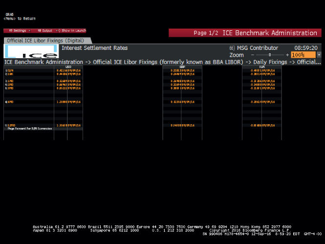
Screenshot illustration of Libor screen on Bloomberg, 13 September 2016. — **FIGURE 1.1** Libor screen on Bloomberg, 13 September 2016.

*Source*: © Bloomberg LP. Used with permission.

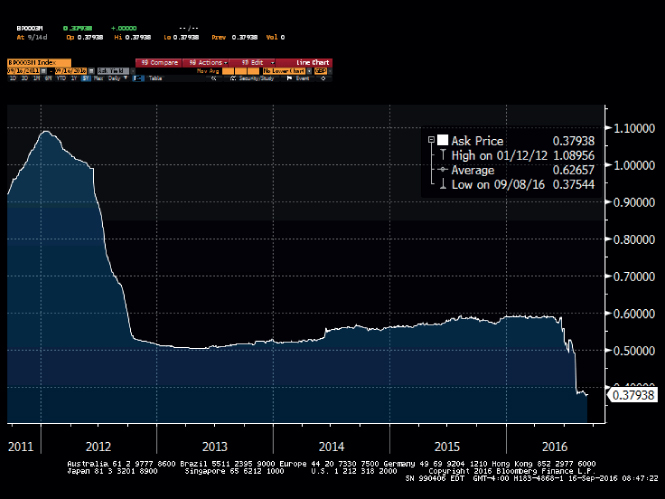
Screenshot illustration of Libor history 2011�2016. — **FIGURE 1.2** Libor history 2011–2016.

*Source*: © Bloomberg LP. Used with permission.

In developed markets, of course, there are usually a range of interest rate indicators. For example, depending on what instrument and market one is concerned with, the sovereign bond interest rates may be worth monitoring, or the overnight index swap (OIS) rate, and so on. It is important to be aware of rates relevant to the balance sheet risk management of your bank, and to understand as well as possible how they interact. Also important is some knowledge of the predictive power of yield curves and how to analyse and interpret them. For illustration, we show the GBP sovereign, interest rate swap, and overnight index swap (SONIA) yield curves for 13 September 2016 at Figure 1.3.

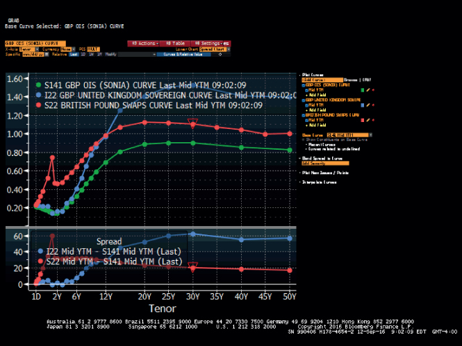
Screenshot illustration of sterling curves, 13 September 2016. — **FIGURE 1.3** Sterling curves, 13 September 2016.

*Source*: © Bloomberg LP. Used with permission.

AN INTRODUCTION TO DEBT FINANCIAL MARKETS

In essence, banks deal in the business of debt, either deposits from customers (banks borrowing from customers), or loans to customers (banks lending to customers). They all “clear” at the end of the day with each other or directly with the central bank.¹ Therefore we introduce the debt money markets and debt capital markets in this first chapter.

This extract from The Money Markets Handbook (2004)

The Money Markets

Part of the global debt capital markets, the money markets are a separate market in their own right. Money market securities are defined as debt instruments with an original maturity of less than one year, although it is common to find that the maturity profile of banks' money market desks runs out to two years.

Money markets exist in every market economy, which is practically every country in the world. They are often the first element of a developing capital market. In every case they are comprised of securities with maturities of up to twelve months. Money market debt is an important part of the global capital markets, and facilitates the smooth running of the banking industry as well as providing working capital for industrial and commercial corporate institutions. The market provides users with a wide range of opportunities and funding possibilities, and the market is characterised by the diverse range of products that can be traded within it. Money market instruments allow issuers, including financial organisations and corporates, to raise funds for short term periods at relatively low interest rates. These issuers include sovereign governments, who issuer Treasury bills, corporates issuing commercial paper and banks issuing bills and certificates of deposit. At the same time investors are attracted to the market because the instruments are highly liquid and carry relatively low credit risk. The Treasury bill market in any country is that country's lowest‐risk instrument, and consequently carries the lowest yield of any debt instrument. Indeed the first market that develops in any country is usually the Treasury bill market. Investors in the money market include banks, local authorities, corporations, money market investment funds and mutual funds and individuals.

In addition to cash instruments, the money markets also consist of a wide range of exchange‐traded and over‐the‐counter off‐balance sheet derivative instruments. These instruments are used mainly to establish future borrowing and lending rates, and to hedge or change existing interest rate exposure. This activity is carried out by both banks, central banks and corporates. The main derivatives are short‐term interest rate futures, forward rate agreements, and short‐dated interest rate swaps such as overnight‐index seaps.

In this chapter we review the cash instruments traded in the money market. In further chapters we review banking asset and liability management, and the market in repurchase agreements. Finally we consider the market in money market derivative instruments including interest‐rate futures and forward‐rate agreements.

Introduction

The cash instruments traded in money markets include the following:

Time deposits;
Treasury Bills;
Certificates of Deposit;
Commercial Paper;
Bankers Acceptances;
Bills of exchange.

In addition money market desks may also trade repo and take part in stock borrowing and lending activities. These products are covered in a separate chapter.

Treasury bills are used by sovereign governments to raise short‐term funds, while certificates of deposit (CDs) are used by banks to raise finance. The other instruments are used by corporates and occasionally banks. Each instrument represents an obligation on the borrower to repay the amount borrowed on the maturity date together with interest if this applies. The instruments above fall into one of two main classes of money market securities: those quoted on a yield basis and those quoted on a discount basis. These two terms are discussed below. A repurchase agreement or “repo” is also a money market instrument and is considered in a separate chapter.

The calculation of interest in the money markets often differs from the calculation of accrued interest in the corresponding bond market. Generally the day‐count convention in the money market is the exact number of days that the instrument is held over the number of days in the year. In the UK sterling market the year base is 365 days, so the interest calculation for sterling money market instruments is given by (1.1):

(1.1)

However the majority of currencies including the US dollar and the euro calculate interest on a 360‐day base so the denominator in (1.1) would be changed accordingly. The process by which an interest rate quoted on one basis is converted to one quoted on the other basis is shown in Appendix 1.1. Those markets that calculate interest based on a 365‐day year are also listed at Appendix 1.1.

Dealers will want to know the interest day‐base for a currency before dealing in it as FX or money markets. Bloomberg users can use screen DCX to look up the number of days of an interest period. For instance, Figure 1.1 shows screen DCX for the US dollar market, for a loan taken out value 7 May 2004 for a straight three‐month period. Ordinarily this would mature on 7 August 2004, however from Figure 1.1 we see that this is not a good day so the loan will actually mature on 9 August 2004. Also from Figure 1.1 we see that this period is actually 94 days, and 92 days under the 30/360 day convention (a bond market accrued interest convention). The number of business days is 64, we also see that there is a public holiday on the 31 May.

For the same loan taken out in Singapore dollars, look at Figure 1.2. This shows that the same loan taken out for value on 7 May will actually mature on 10 August, because 9 August 2004 is a public holiday in that market.

Figure 1.1 Bloomberg screen DCX used for US dollar market, three‐month loan taken out 7 May 2004

Figure 1.2 Bloomberg screen DCX for Singapore dollar market, three‐month loan taken out 7 May 2004

Settlement of money market instruments can be for value today (generally only when traded in before mid‐day), tomorrow or two days forward, known as spot.

Figure 1.3 London sterling money market rates. Extract from Financial Times, 11 March 2004.

Securities quoted on a yield basis

Two of the instruments in the list above are yield‐based instruments.

Money market deposits

These are fixed‐interest term deposits of up to one year with banks and securities houses. They are also known as time deposits or clean deposits. They are not negotiable so cannot be liquidated before maturity. The interest rate on the deposit is fixed for the term and related to the London Interbank Offer Rate (LIBOR) of the same term. Interest and capital are paid on maturity.

Certificates of Deposit

Certificates of Deposit (CDs) are receipts from banks for deposits that have been placed with them. They were first introduced in the US dollar market in 1964, and in the sterling market in 1958. The deposits themselves carry a fixed rate of interest related to LIBOR and have a fixed term to maturity, so cannot be withdrawn before maturity. However the certificates themselves can be traded in a secondary market, that is, they are negotiable.¹ CDs are therefore very similar to negotiable money market deposits, although the yields are about 0.15% below the equivalent deposit rates because of the added benefit of liquidity. Most CDs issued are of between one and three months' maturity, although they do trade in maturities of one to five years. Interest is paid on maturity except for CDs lasting longer than one year, where interest is paid annually or occasionally, semi‐annually.

Banks, merchant banks and building societies issue CDs to raise funds to finance their business activities. A CD will have a stated interest rate and fixed maturity date and can be issued in any denomination. On issue a CD is sold for face value, so the settlement proceeds of a CD on issue are always equal to its nominal value. The interest is paid, together with the face amount, on maturity. The interest rate is sometimes called the coupon,but unless the CD is held to maturity this will not equal the yield, which is of course the current rate available in the market and varies over time. The largest group of CD investors are banks, money market funds, corporates and local authority treasurers.

Unlike coupons on bonds, which are paid in rounded amounts, CD coupon is calculated to the exact day.

CD yields

The coupon quoted on a CD is a function of the credit quality of the issuing bank, and its expected liquidity level in the market, and of course the maturity of the CD, as this will be considered relative to the money market yield curve. As CDs are issued by banks as part of their short‐term funding and liquidity requirement, issue volumes are driven by the demand for bank loans and the availability of alternative sources of funds for bank customers. The credit quality of the issuing bank is the primary consideration however; in the sterling market the lowest yield is paid by “clearer” CDs, which are CDs issued by the clearing banks such as Royal Bank of Scotland, HSBC and Barclays Bank plc. In the US market “prime” CDs, issued by highly‐rated domestic banks, trade at a lower yield than non‐prime CDs. In both markets CDs issued by foreign banks such as French or Japanese banks will trade at higher yields.

Euro‐CDs, which are CDs issued in a different currency to that of the home currency, also trade at higher yields, in the US because of reserve and deposit insurance restrictions.

If the current market price of the CD including accrued interest is P and the current quoted yield is r, the yield can be calculated given the price, using (1.2):

(1.2)

The price can be calculated given the yield using (1.3):

(1.3)

Where

C	is the quoted coupon on the CD
M	is the face value of the CD
B	is the year day‐basis (365 or 360)
F	is the maturity value of the CD
N_im	is the number of days between issue and maturity
N_sm	is the number of days between settlement and maturity
N_is	is the number of days between issue and settlement.

After issue a CD can be traded in the secondary market. The secondary market in CDs in developed economies is very liquid, and CDs will trade at the rate prevalent at the time, which will invariably be different from the coupon rate on the CD at issue. When a CD is traded in the secondary market, the settlement proceeds will need to take into account interest that has accrued on the paper and the different rate at which the CD has now been dealt. The formula for calculating the settlement figure is given at (1.4) which applies to the sterling market and its 365‐day count basis.

(1.4)

The settlement figure for a new issue CD is of course, its face value…!²

The tenor of a CD is the life of the CD in days, while days remaining is the number of days left to maturity from the time of trade.

The return on holding a CD is given by (1.5):

(1.5)

US Dollar market rates

Treasury Bills

The Treasury bill market in the United States is the most liquid and transparent debt market in the world. Consequently the bid‐offer spread on them is very narrow. The Treasury issues bills at a weekly auction each Monday, made up of 91‐day and 182‐day bills. Every fourth week the Treasury also issues 52‐week bills as well. As a result there are large numbers of Treasury bills outstanding at any one time. The interest earned on Treasury bills is not liable to state and local income taxes. T‐bill rates are the lowest in the dollar market (as indeed any bill market is in respective domestic environment) and as such represents the corporate financier's risk‐free interest rate.

Federal Funds

Commercial banks in the US are required to keep reserves on deposit at the Federal Reserve. Banks with reserves in excess of required reserves can lend these funds to other banks, and these interbank loans are called federal funds or fed funds and are usually overnight loans. Through the fed funds market, commercial banks with excess funds are able to lend to banks that are short of reserves, thus facilitating liquidity. The transactions are very large denominations, and are lent at the fed funds rate, which is a very volatile interest rate because it fluctuates with market shortages.

Prime Rate

The prime interest rate in the US is often said to represent the rate at which commercial banks lend to their most creditworthy customers. In practice many loans are made at rates below the prime rate, so the prime rate is not the best rate at which highly rated firms may borrow. Nevertheless the prima rate is a benchmark indicator of the level of US money market rates, and is often used as a reference rate for floating‐rate instruments. As the market for bank loans is highly competitive, all commercial banks quote a single prime rate, and the rate for all banks changes simultaneously.

Securities quoted on a discount basis

The remaining money market instruments are all quoted on a discount basis, and so are known as “discount” instruments. This means that they are issued on a discount to face value, and are redeemed on maturity at face value. Treasury bills, bills of exchange, bankers acceptances and commercial paper are examples of money market securities that are quoted on a discount basis, that is, they are sold on the basis of a discount to par. The difference between the price paid at the time of purchase and the redemption value (par) is the interest earned by the holder of the paper. Explicit interest is not paid on discount instruments, rather interest is reflected implicitly in the difference between the discounted issue price and the par value received at maturity.

Treasury bills

Treasury bills or T‐bills are short‐term government “IOUs” of short duration, often three‐month maturity. For example if a bill is issued on 10 January it will mature on 10 April. Bills of one‐month and six‐month maturity are issued in certain markets, but only rarely by the UK Treasury. On maturity the holder of a T‐Bill receives the par value of the bill by presenting it to the Central Bank. In the UK most such bills are denominated in sterling but issues are also made in euros. In a capital market, T‐Bill yields are regarded as the risk‐free yield, as they represent the yield from short‐term government debt. In emerging markets they are often the most liquid instruments available for investors.

A sterling T‐bill with £10 million face value issued for 91 days will be redeemed on maturity at £10 million. If the three‐month yield at the time of issue is 5.25%, the price of the bill at issue is:

In the UK market the interest rate on discount instruments is quoted as a discount rate rather than a yield. This is the amount of discount expressed as an annualised percentage of the face value, and not as a percentage of the original amount paid. By definition the discount rate is always lower than the corresponding yield. If the discount rate on a bill is d, then the amount of discount is given by (1.12):

(1.12)

where B is the day‐count basis.

The price P paid for the bill is the face value minus the discount amount, given by (1.13):

(1.13)

If we know the yield on the bill then we can calculate its price at issue by using the simple present value formula, as shown at (1.14):

(1.14)

The discount rate d for T‐Bills is calculated using (1.15):

(1.15)

where n is the T‐bill number of days.

The relationship between discount rate and true yield is given by (1.16):

(1.16)

If a T‐Bill is traded in the secondary market, the settlement proceeds from the trade are calculated using (1.17):

(1.17)

Reproduced from The Money Markets Handbook (2004)

This extract from The Money Markets Handbook (2004)

Foreign Exchange Markets

The market in foreign exchange is an excellent example of a liquid, transparent and immediate global financial market. Rates in the foreign exchange (FX) markets move at an extremely rapid pace and in fact, trading in FX is a different discipline to bond trading or money markets trading. There is a considerable literature on the FX markets, as it is a separate subject in its own right. However some banks organise their forward FX desk as part of the money market desk and not the foreign exchange desk, necessitating its inclusion in this book. For this reason we present an overview summary of FX in this chapter, both spot and forward.

The quotation for currencies generally follows the ISO convention, which is also used by the SWIFT and Reuters dealing systems, and is the three‐letter code used to identify a currency, such as USD for US dollar and GBP for sterling. The rate convention is to quote everything in terms of one unit of the US dollar, so that the dollar and Swiss franc rate is quoted as USD/CHF, and is the number of Swiss francs to one US dollar. The exception is for sterling, which is quoted as GBP/USD and is the number of US dollars to the pound. This rate is also known as “cable”. The rate for euros has been quoted both ways round, for example EUR/USD although some banks, for example Royal Bank of Scotland in the UK, quote euros to the pound, that is GBP/EUR.

The complete list of currency codes was given at Appendix 1.2.

Spot exchange rates

A spot FX trade is an outright purchase or sale of one currency against another currency, with delivery two working days after the trade date. Non‐working days so not count, so a trade on a Friday is settled on the following Tuesday. There are some exceptions to this, for example trades of US dollar against Canadian dollar are settled the next working day; note that in some currencies, generally in the Middle‐East, markets are closed on Friday but open on Saturday. A settlement date that falls on a public holiday in the country of one of the two currencies is delayed for settlement by that day. An FX transaction is possible between any two currencies, however to reduce the number of quotes that need to be made the market generally quotes only against the US dollar or occasionally against sterling or euro, so that the exchange rate between two non‐dollar currencies is calculated from the rate for each currency against the dollar. The resulting exchange rate is known as the cross‐rate. Cross‐rates themselves are also traded between banks in addition to dollar‐based rates. This is usually because the relationship between two rates is closer than that of either against the dollar, for example the Swiss franc moves more closely in line with the euro than against the dollar, so in practice one observes that the dollar / Swiss franc rate is more a function of the euro / franc rate.

The spot FX quote is a two‐way bid‐offer price, just as in the bond and money markets, and indicates the rate at which a bank is prepared to buy the base currency against the variable currency; this is the “bid” for the variable currency, so is the lower rate. The other side of the quote is the rate at which the bank is prepared to sell the base currency against the variable currency. For example a quote of 1.6245 ‐ 1.6255 for GBP/USD means that the bank is prepared to buy sterling for $1.6245, and to sell sterling for $1.6255. The convention in the FX market is uniform across countries, unlike the money markets. Although the money market convention for bid‐offer quotes is for example, 5½% ‐ 5¼%, meaning that the “bid” for paper ‐ the rate at which the bank will lend funds, say in the CD market ‐ is the higher rate and always on the left, this convention is reversed in certain countries. In the FX markets the convention is always the same one just described.

The difference between the two side in a quote is the bank's dealing spread. Rates are quoted to 1/100^th of a cent, known as a pip. In the quote above, the spread is 10 pips, however this amount is a function of the size of the quote number, so that the rate for USD/JPY at say, 110.10 ‐ 110.20, indicates a spread of 0.10 yen. Generally only the pips in the two rates are quoted, so that for example the quote above would be simply “45‐55”. The “big figure” is not quoted.

The derivation of cross‐rates can be depicted in the following way. If we assume two exchange rates XXX/YYY and XXX/ZZZ, the cross‐rates are:

Given two exchange rates YYY/XXX and XXX/ZZZ, the cross‐rates are:

Figure 2.1 shows the Bloomberg major currency FX monitor, page FXC, as at 10 May 2004.

Figure 2.1 Bloomberg major currency monitor page, 10 May 2004

Forward exchange rates

Forward outright

The spot exchange rate is the rate for immediate delivery (notwithstanding that actual delivery is two days forward). A forward contract or simply forward is an outright purchase or sale of one currency in exchange for another currency for settlement on a specified date at some point in the future. The exchange rate is quoted in the same way as the spot rate, with the bank buying the base currency on the bid side and selling it on the offered side. In some emerging markets no liquid forward market exists so forwards are settled in cash against the spot rate on the maturity date. These non‐deliverable forwards are considered at the end of this section.

Although some commentators have stated that the forward rate may be seen as the market's view of where the spot rate will be on the maturity date of the forward transaction, this is incorrect. A forward rate is calculated on the current interest rates of the two currencies involved, and the principle of no‐arbitrage pricing ensures that there is no profit to be gained from simultaneous (and opposite) dealing in spot and forward. Consider the following strategy:

borrow US dollars for six months starting from the spot value date;
sell dollars and buy sterling for value spot;
deposit the long sterling position for six months from the spot value date;
sell forward today the sterling principal and interest which mature in six months time into dollars.

The market will adjust the forward price so that the two initial transactions if carried out simultaneously will generate a zero profit/loss. The forward rates quoted in the trade will be calculated on the six months deposit rates for dollars and sterling; in general the calculation of a forward rate is given as (2.1)

(2.1)

The year day‐count base B will be either 365 or 360 depending on the convention for the currency in question.

So in other words, a forward is more a deposit instrument than an FX instrument.

Example 2.2 Forward rate arbitrage

The following rates are quoted to a bank:

The bank requires funding of CHF10 million for three months (91 days). It deals on the above rates and actions the following:

it borrows USD 6,749,915,63 for 91 days from spot at 7.56%
at the end of the 91 days the bank repays the principal plus the interest, which is a total of USD 6,880,324.00
the bank “buys and sells” USD against CHF at a swap price of 11, based on the spot rate of 1.4815, that is:
- the bank sells USD 6,749,915.63/buys CHF10 million spot at 1.4815;
- the bank buys USD 6,880,324/sells CHF 10,116,828.42 for three months forward at 1.4704;

The net USD cash flows result in a zero balance.

The effective cost of borrowing is therefore interest of CHF 116,828.41 on a principal sum of CHF10 million for 91 days, which is:

The net effect is therefore a CHF10 million borrowing at 4.57%, which is 5 basis points lower than the 4.62% quote at which the bank could borrow directly in the market. If the bank has not actually required funding but was able to deposit the Swiss francs at a higher rate than 4.57%, it would have been able to lock in a profit.

Forward swaps

The calculation given above illustrates how a forward rate is calculated and quoted in theory. In practice as spot rates change rapidly, often many times even in one minute, it would be tedious to keep re‐calculating the forward rate so often. Therefore banks quote a forward spread over the spot rate, which can then be added or subtracted to the spot rate as it changes. This spread is known as the swap points. An approximate value for the number of swap points is given by (2.2) below.

(2.2)

The approximation is not accurate enough for forwards maturing more than 30 days from now, in which case another equation must be used. This is given as (2.3). It is also possible to calculate an approximate deposit rate differential from the swap points by re‐arranging 2.2.

(2.3)

The swap points are quoted as two‐way prices in the same way as spot rates. In practice a middle spot price is used and then the forward swap spread around the spot quote. The difference between the interest rates of the two currencies will determine the magnitude of the swap points and whether they are added or subtracted from the spot rate. When the swap points are positive and the forwards trader applies a bid‐offer spread to quote a two‐way price, the left‐hand side of the quote is smaller than the right‐hand side as usual. When the swap points are negative, the trader must quote a “more negative” number on the left and a “more positive” number on the right‐hand side. The “minus” sign is not shown however, so that the left‐hand side may appear to be the larger number. Basically when the swap price appears larger on the right, it means that it is negative and must be subtracted from the spot rate and not added.

Forwards traders are in fact interest rate traders rather than foreign exchange traders; although they will be left with positions that arise from customer orders, in general they will manage their book based on their view of short‐term deposit rates in the currencies they are trading. In general a forward trader expecting the interest rate differential to move in favour of the base currency, for example, a rise in base currency rates or a fall in the variable currency rate, will “buy and sell” the base currency. This is equivalent to borrowing the base currency and depositing in the variable currency. The relationship between interest rates and forward swaps means that banks can take advantage of different opportunities in different markets. Assume that a bank requires funding in one currency but is able to borrow in another currency at a relatively cheaper rate. It may wish to borrow in the second currency and use a forward contract to convert the borrowing to the first currency. It will do this if the all‐in cost of borrowing is less than the cost of borrowing directly in the first currency.

Forward cross‐rates

A forward cross‐rate is calculated in the same way as spot cross‐rates. The formulas given for spot cross‐rates can be adapted to forward rates.

Forward‐forwards

A forward‐forward swap is a deal between two forward dates rather than from the spot date to a forward date; this is the same terminology and meaning as in the bond markets, where a forward or a forward‐forward interest rate is the zero‐coupon interest rate between two points both beginning in the future. In the foreign exchange market, an example would be a contract to sell sterling three months forward and buy it back in six months time. Here, the swap is for the three‐month period between the three‐month date and the six‐month date. The reason a bank or corporate might do this is to hedge a forward exposure or because of a particular view it has on forward rates, in effect deposit rates.

Example 2.4 Forward‐forward contract

If a bank wished to sell GBP three month forward and buy it back six months forward, this is identical to undertaking one swap to buy GBP spot and sell GBP three months forward, and another to sell GBP spot and buy it six months forward. Swaps are always quoted as the quoting bank buying the base currency forward on the bid side, and selling the base currency forward on the offered side; the counterparty bank can “buy and sell” GBP “spot against three months” at a swap price of −45, with settlement rates of spot and (spot − 0.0045). It can “sell and buy” GBP “spot against six months” at the swap price of −125 with settlement rates of spot and (spot − 0.0125). It can therefore do both simultaneously, which implies a difference between the two forward prices of (−125) − (−45) = −90 points. Conversely the bank can “buy and sell” GBP “three months against six months” at a swap price of (−135) − (−41) or −94 points. The two‐way price is therefore 94–90 (we ignore the negative signs).

Long‐dated forward contracts

The formula for calculating a forward rate was given earlier (see 2.2). This formula applies to any period that is under one year, hence the adjustment of the deposit rate by the fraction of the day‐count. However if a forward contract is traded for a period greater than one year, the formula must be adjusted to account for the fact that deposit rates are compounded if they are in effect for more than one year. To calculate a long‐dated forward rate, in theory (2.4) should be used. In practice the formula may not give an answer to the required accuracy, because it does not consider reinvestment risk. To get around this it is necessary to use spot (zero‐coupon) rates in the formula. However the market in long‐dated forward contracts is not as liquid as the sub‐1‐year market, so banks may not be as keen to quote a price.

(2.4)

where N is the contract's maturity in years.

Reproduced from The Money Markets Handbook (2004)

This extract from Fixed Income Markets, Second Edition (2014)

The Bond Instrument

Bonds are debt‐capital market instruments that represent a cash flow payable during a specified time period heading into the future. This cash flow represents the interest payable on the loan and the loan redemption. So, essentially, a bond is a loan, albeit one that is tradable in a secondary market. This differentiates bond‐market securities from commercial bank loans.

In the analysis that follows, bonds are assumed to be default‐free, which means that there is no possibility that the interest payments and principal repayment will not be made. Such an assumption is reasonable when one is referring to government bonds such as U.S. Treasuries, UK gilts, Japanese JGBs, and so on. However, it is unreasonable when applied to bonds issued by corporates or lower‐rated sovereign borrowers. Nevertheless, it is still relevant to understand the valuation and analysis of bonds that are default‐free, as the pricing of bonds that carry default risk is based on the price of risk‐free securities. Essentially, the price investors charge borrowers that are not of risk‐free credit standing is the price of government securities plus some credit risk premium.

BOND MARKET BASICS

All bonds are described in terms of their issuer, maturity date, and coupon. For a default‐free conventional, or plain‐vanilla, bond, this will be the essential information required. Nonvanilla bonds are defined by further characteristics such as their interest basis, flexibilities in their maturity date, credit risk, and so on.

Figure 1.1 shows screen DES from the Bloomberg system. This page describes the key characteristics of a bond. From Figure 1.1, we see a description of a bond issued by the Singapore government, the 4.625% of 2010. This tells us the following bond characteristics:

Issue date	July 2000
Coupon	4.625%
Maturity date	1 July 2010
Issue currency	Singapore dollars
Issue size	SGD 3.4 million
Credit rating	AAA/Aaa

Figure 1.1 Bloomberg Screen DES Showing Details of 4⅝ % 2010 Issued by Republic of Singapore as of 20 October 2003

Calling up screen DES for any bond, provided it is supported by Bloomberg, will provide us with its key details. Later on, we will see how nonvanilla bonds include special features that investors take into consideration in their analysis.

We will consider the essential characteristics of bonds later in this chapter. First, we review the capital market, and an essential principle of finance, the time value of money.

CAPITAL MARKET PARTICIPANTS

The debt capital markets exist because of the financing requirements of governments and corporates. The source of capital is varied, but the total supply of funds in a market is made up of personal or household savings, business savings, and increases in the overall money supply. Growth in the money supply is a function of the overall state of the economy, and interested readers may wish to consult the references at the end of this chapter, which include several standard economic texts. Individuals save out of their current income for future consumption, while business savings represent retained earnings. The entire savings stock represents the capital available in a market. The requirements of savers and borrowers differ significantly, in that savers have a short‐term investment horizon while borrowers prefer to take a longer‐term view. The constitutional weakness of what would otherwise be unintermediated financial markets led, from an early stage, to the development of financial intermediaries.

Financial Intermediaries

In its simplest form a financial intermediary is a broker or agent. Today we would classify the broker as someone who acts on behalf of the borrower or lender, buying or selling a bond as instructed. However, intermediaries originally acted between borrowers and lenders in placing funds as required. A broker would not simply on‐lend funds that have been placed with it, but would accept deposits and make loans as required by its customers. This resulted in the first banks. A retail bank deals mainly with the personal financial sector and small businesses, and in addition to loans and deposits also provides cash transmission services. A retail bank is required to maintain a minimum cash reserve, to meet potential withdrawals, but the remainder of its deposit base can be used to make loans. This does not mean that the total size of its loan book is restricted to what it has taken in deposits: loans can also be funded in the wholesale market. An investment bank will deal with governments, corporates, and institutional investors. Investment banks perform an agency role for their customers, and are the primary vehicle through which a corporate will borrow funds in the bond markets. This is part of the bank's corporate finance function; it will also act as wholesaler in the bond markets, a function known as market making. The bond‐issuing function of an investment bank, by which the bank will issue bonds on behalf of a customer and pass the funds raised to this customer, is known as origination. Investment banks will also carry out a range of other functions for institutional customers, including export finance, corporate advisory, and fund management.

Other financial intermediaries will trade not on behalf of clients but for their own book. These include arbitrageurs and speculators. Usually such market participants form part of investment banks.

Investors

There is a large variety of players in the bond markets, each trading some or all of the different instruments available to suit their own purposes. We can group the main types of investors according to the time horizon of their investment activity.

Short‐term institutional investors. These include banks and building societies, money‐market fund managers, central banks, and the treasury desks of some types of corporates. Such bodies are driven by short‐term investment views, often subject to close guidelines, and will be driven by the total return available on their investments. Banks will have an additional requirement to maintain liquidity, often in fulfilment of regulatory authority rules, by holding a proportion of their assets in the form of easily tradable short‐term instruments.

Long‐term institutional investors. Typically these types of investors include pension funds and life assurance companies. Their investment horizon is long term, reflecting the nature of their liabilities; often they will seek to match these liabilities by holding long‐dated bonds.

Mixed horizon institutional investors. This is possibly the largest category of investors and will include general insurance companies, most corporate bodies, and sovereign wealth funds. Like banks and financial‐sector companies, they are also very active in the primary market, issuing bonds to finance their operations.

Market professionals. This category includes the banks and specialist financial intermediaries mentioned earlier, firms that one would not automatically classify as “investors” although they will also have an investment objective. Their time horizon will range from one day to the very long term. Proprietary traders will actively position themselves in the market in order to gain trading profit, for example in response to their view on where they think interest rate levels are headed. These participants will trade directly with other market professionals and investors, or via brokers. Market makers or traders (called dealers in the United States) are wholesalers in the bond markets; they make two‐way prices in selected bonds. Firms will not necessarily be active market makers in all types of bonds; smaller firms often specialise in certain sectors. In a two‐way quote the bid price is the price at which the market maker will buy stock, so it is the price the investor will receive when selling stock. The offer price or ask price is the price at which investors can buy stock from the market maker. As one might expect, the bid price is always higher than the offer price, and it is this spread that represents the theoretical profit to the market maker. The bid‐offer spread set by the marketmaker is determined by several factors, including supply and demand, and liquidity considerations for that particular stock, the trader's view on market direction and volatility as well as that of the stock itself and the presence of any market intelligence. A large bid‐offer spread reflects low liquidity in the stock, as well as low demand.

Markets

Markets are that part of the financial system where capital market transactions, including the buying and selling of securities, takes place. A market can describe a traditional stock exchange; that is, a physical trading floor where securities trading occurs. Many financial instruments are traded over the telephone or electronically; these markets are known as over‐the‐counter (OTC) markets. A distinction is made between financial instruments of up to one year's maturity and instruments of over one year's maturity. Short‐term instruments make up the money market while all other instruments are deemed to be part of the capital market. There is also a distinction made between the primary market and the secondary market. A new issue of bonds made by an investment bank on behalf of its client is made in the primary market. Such an issue can be a public offer, in which anyone can apply to buy the bonds, or a private offer where the customers of the investment bank are offered the stock. The secondary market is the market in which existing bonds and shares are subsequently traded.

Table 1.1 Selected Government Bond Market Characteristics

	Credit Rating	Maturity Range	Dealing Mechanism	Benchmark Bonds	Issuance	Coupon and Day‐Count Basis
Australia	AAA	2–15 years	OTC Dealer network	5, 10 years	Auction	Semiannual, act/act
Canada	AAA	2–30 years	OTC Dealer network	3, 5, 10 years	Auction, subscription	Semiannual, act/act
France	AAA	BTAN: 1–7 years OAT: 10–30 years	OTC Dealer network Bonds listed on Paris Stock Exchange	BTAN: 2, 5 years OAT: 10, 30 years	Dutch auction	BTAN: Semiannual, act/act OAT: Annual, act/act
Germany	AAA	OBL: 2, 5 years BUND: 10, 30 years	OTC Dealer network Listed on Stock Exchange	The most recent issue	Combination of Dutch auction and proportion of each issue allocated on fixed basis to institutions	Annual, act/act
South Africa	A	2–30 years	OTC Dealer network Listed on Johannesburg SE	2, 7, 10, 20 years	Auction	Semiannual, act/365
Singapore	AAA	2–15 years	OTC Dealer network	1, 5, 10, 15 years	Auction	Semiannual, act/act
Taiwan	AA–	2–30 years	OTC Dealer network	2, 5, 10, 20, 30 years	Auction	Annual, act/act
United Kingdom	AAA	2–50 years	OTC Dealer network	5, 10, 30 years	Auction, subsequent issue by “tap” subscription	Semiannual, act/act
United States	AAA	2–20 years	OTC Dealer network	2, 5, 10 years	Auction	Semiannual, act/act

Table 1.2 Selected Government Bond Markets, Yield Curves as at 2 December 2013

Source: Bloomberg LP.

Term (years)	Australia	Germany	Japan	United Kingdom	United States
1				0.43	0.110
2	2.74	0.12	0.08	0.48	0.250
3
4
5	3.49	0.66	0.18	1.58	1.251
7
10	4.32	1.7	0.61	2.83	2.753
15	4.63			3.17
20				3.36
30		2.62	1.65	3.64	3.756

BOND PRICING AND YIELD: THE TRADITIONAL APPROACH

Bond Pricing

The interest rate that is used to discount a bond's cash flows (and therefore called the discount rate) is the rate required by the bondholder. This is therefore known as the bond's yield. The yield on the bond will be determined by the market and is the price demanded by investors for buying it, which is why it is sometimes called the bond's return. The required yield for any bond will depend on a number of political and economic factors, including what yield is being earned by other bonds of the same class. Yield is always quoted as an annualised interest rate, so that for a bond paying semiannually exactly half of the annual rate is used to discount the cash flows.

The fair price of a bond is the present value of all its cash flows. Therefore, when pricing a bond, we need to calculate the present value of all the coupon interest payments and the present value of the redemption payment, and sum these. The price of a conventional bond that pays annual coupons can therefore be given by (1.11).

(1.11)

Where	P	is the price
	C	is the annual coupon payment
	r	is the discount rate (therefore, the required yield)
	N	is the number of years to maturity (therefore, the number of interest periods in an annually paying bond)
	M	is the maturity payment or par value (usually 100% of currency)

Note that (1.11) applies only for fixed coupon bonds where the “recovery rate” (RR) on default of the issuer is zero. In other words, we can only assume it for default‐risk free bonds. The RR term will be explained and considered in later chapters.

For long‐hand calculation purposes, the first half of (1.11) is usually simplified and is sometimes encountered in one of the two ways shown in (1.12).

(1.12)

The price of a bond that pays semiannual coupons is given by the expression in (1.13), which is our earlier expression modified to allow for the twice‐yearly discounting:

(1.13)

Note how we set 2N as the power to which to raise the discount factor, as there are two interest payments every year for a bond that pays semiannually. Therefore, a more convenient function to use might be the number of interest periods in the life of the bond, as opposed to the number of years to maturity, which we could set as n, allowing us to alter the equation for a semiannually paying bond as:

(1.14)

The formula in (1.14) calculates the fair price on a coupon‐payment date, so that there is no accrued interest incorporated into the price. It also assumes that there is an even number of coupon‐payment dates remaining before maturity. The concept of accrued interest is an accounting convention, and treats coupon interest as accruing every day that the bond is held; this amount is added to the discounted present value of the bond (the clean price) to obtain the market value of the bond, known as the dirty price.

The date used as the point for calculation is the settlement date for the bond, the date on which a bond will change hands after it is traded. For a new issue of bonds, the settlement date is the day when the stock is delivered to investors and payment is received by the bond issuer. The settlement date for a bond traded in the secondary market is the day when the buyer transfers payment to the seller of the bond and when the seller transfers the bond to the buyer. Different markets will have different settlement conventions. For example, Australian government bonds normally settle two business days after the trade date (the notation used in bond markets is “T + 2”), whereas Eurobonds settle on T + 3. The term value date is sometimes used in place of settlement date. However, the two terms are not strictly synonymous. A settlement date can only fall on a business date, so that an Australian government bond traded on a Friday will settle on a Tuesday. However, a value date can sometimes fall on a non‐business day; for example, when accrued interest is being calculated.

The standard formula also assumes that the bond is traded for a settlement on a day that is precisely one interest period before the next coupon payment. The price formula is adjusted if dealing takes place in between coupon dates. If we take the value date for any transaction, we then need to calculate the number of calendar days from this day to the next coupon date. We then use the following ratio i when adjusting the exponent for the discount factor:

The number of days in the interest period is the number of calendar days between the last coupon date and the next one, and it will depend on the day‐count basis used for that specific bond. The price formula is then modified as shown in (1.15).

(1.15)

where the variables C, M, n and r are as before. Note that (1.15) assumes r for an annually paying bond and is adjusted to r/2 for a semiannually paying bond.

Example 1.1

In these examples we illustrate the long‐hand price calculation, using both expressions for the calculation of the present value of the annuity stream of a bond's cash flows.

1.1 (A)

Calculate the fair pricing of a U.S. Treasury, the 4% of February 2014, which pays semiannual coupons, with the following terms:

The fair price of the Treasury is $99 − 19+, which is composed of the present value of the stream of coupon payments ($32.628) and the present value of the return of the principal ($66.981).

This yield calculation is shown at Figure 1.3, the Bloomberg YA page for this security. We show the price shown as 99 − 19+ for settlement on 17 Feb 2004, the date it was issued.

Figure 1.3 Bloomberg YA Page for Yield Analysis

1.1(B)

What is the price of a 5% coupon sterling bond with precisely five years to maturity, with semiannual coupon payments, if the yield required is 5.40%?

As the cash flows for this bond are 10 semiannual coupons of £2.50 and a redemption payment of £100 in 10 six‐month periods from now, the price of the bond can be obtained by solving the following expression, where we substitute C = 2.5, n = 10, and r = 0.027 into the price equation (the values for C and r reflect the adjustments necessary for a semiannual paying bond).

The price of the bond is $98.2675 per $100 nominal.

1.1(C)

What is the price of a 5% coupon euro bond with five years to maturity paying annual coupons, again with a required yield of 5.4%?

In this case there are five periods of interest, so we may set C = 5, n = 5, with r = 0.05.

Note how the annual‐paying bond has a slightly higher price for the same required annualised yield. This is because the semiannual paying sterling bond has a higher effective yield than the euro bond, resulting in a lower price.

1.1(D)

Consider our 5% sterling bond again, but this time the required yield has risen and is now 6%. This makes C = 2.5, n = 10, and r = 0.03.

As the required yield has risen, the discount rate used in the price calculation is now higher, and the result of the higher discount is a lower present value (price).

1.1(E)

Calculate the price of our sterling bond, still with five years to maturity but offering a yield of 5.1%.

To satisfy the lower required yield of 5.1%, the price of the bond has fallen to £99.56 per £100.

1.1(F)

Calculate the price of the 5% sterling bond one year later, with precisely four years left to maturity and with the required yield still at the original 5.40%. This sets the terms in 1.1(b) unchanged, except now n = 8.

The price of the bond is £98.58. Compared to 1.1(B) this illustrates how, other things being equal, the price of a bond will approach par (£100 percent) as it approaches maturity.

There also exist perpetual or irredeemable bonds which have no redemption date, so that interest on them is paid indefinitely. They are also known as undated bonds. An example of an undated bond is the 3½% War Loan, a UK gilt originally issued in 1916 to help pay for the 1914–1918 war effort. Most undated bonds date from a long time in the past, and it is unusual to see them issued today. In structure, the cash flow from an undated bond can be viewed as a continuous annuity. The fair price of such a bond is given from (1.11) by setting N = ∞, such that:

(1.16)

In most markets, bond prices are quoted in decimals, in minimum increments of 1/100ths. This is the case with Eurobonds, euro‐denominated bonds, and gilts, for example. Certain markets—including the U.S. Treasury market and South African and Indian government bonds, for example—quote prices in ticks, where the minimum increment is 1/32nd. One tick is therefore equal to 0.03125. A U.S. Treasury might be priced at “98‐05” which means “98 and five ticks”. This is equal to 98 and 5/32nds which is 98.15625.

Bonds that do not pay a coupon during their life are known as zero‐coupon bonds or strips, and the price for these bonds is determined by modifying (1.11) to allow for the fact that C = 0. We know that the only cash flow is the maturity payment, so we may set the price as:

(1.17)

where M and r are as before and N is the number of years to maturity. The important factor is to allow for the same number of interest periods as coupon bonds of the same currency. That is, even though there are no actual coupons, we calculate prices and yields on the basis of a quasi‐coupon period. For a U.S. dollar or a sterling zero‐coupon bond, a five‐year zero coupon bond would be assumed to cover 10 quasi‐coupon periods, which would set the price equation as:

(1.18)

We have to note carefully the quasi‐coupon periods in order to maintain consistency with conventional bond pricing.

An examination of the bond price formula tells us that the yield and price for a bond are related. A key aspect of this relationship is that the price changes in the opposite direction to the yield. This is because the price of the bond is the net present value of its cash flows; if the discount rate used in the present value calculation increases, the present values of the cash flows will decrease. This occurs whenever the yield level required by bondholders increases. In the same way, if the required yield decreases, the price of the bond will rise. This property was observed in Example 1.2. As the required yield decreased, the price of the bond increased, and we observed the same relationship when the required yield was raised.

The relationship between any bond's price and yield at any required yield level is illustrated in a stylised manner in Figure 1.4, which is obtained if we plot the yield against the corresponding price; this shows a convex curve. In practice the curve is not quite as perfectly convex as illustrated in Figure 1.4, but the diagram is representative.

Figure 1.4 The Price/Yield Relationship

BOND YIELD

We have observed how to calculate the price of a bond using an appropriate discount rate known as the bond's yield. We can reverse this procedure to find the yield of a bond where the price is known, which would be equivalent to calculating the bond's internal rate of return (IRR). The IRR calculation is taken to be a bond's yield to maturity or redemption yield and is one of various yield measures used in the markets to estimate the return generated from holding a bond. In most markets, bonds are generally traded on the basis of their prices, but because of the complicated patterns of cash flows that different bonds can have they are generally compared in terms of their yields. This means that a marketmaker will usually quote a two‐way price at which she will buy or sell a particular bond, but it is the yield at which the bond is trading that is important to the marketmaker's customer. This is because a bond's price does not actually tell us anything useful about what we are getting. Remember, that in any market there will be a number of bonds with different issuers, coupons, and terms to maturity. Even in a homogenous market such as the Treasury market, different bonds and notes will trade according to their own specific characteristics. To compare bonds in the market, therefore, we need the yield on any bond, and it is yields that we compare, not prices.

The yield on any investment is the interest rate that will make the present value of the cash flows from the investment equal to the initial cost (price) of the investment. Mathematically, the yield on any investment, represented by r, is the interest rate that satisfies (1.19), which is simply the bond price equation we've already reviewed.

(1.19)

But as we have noted there are other types of yield measure used in the market for different purposes. The simplest measure of the yield on a bond is the current yield, also known as the flat yield, interest yield or running yield. The running yield is given by (1.20).

(1.20)

where rc is the current yield.

In (1.20) C is not expressed as a decimal. Current yield ignores any capital gain or loss that might arise from holding and trading a bond and does not consider the time value of money. It essentially calculates the bond coupon income as a proportion of the price paid for the bond, and to be accurate would have to assume that the bond was more like an annuity rather than a fixed‐term instrument.

The current yield is useful as a rough‐and‐ready interest‐rate calculation; it is often used to estimate the cost of or profit from a short‐term holding of a bond. For example, if other short‐term interest rates such as the one‐week or three‐month rates are higher than the current yield, holding the bond is said to involve a running cost. This is also known as negative carry or negative funding. The term is used by bond traders and market makers and leveraged investors. The carry on a bond is a useful measure for all market practitioners as it illustrates the cost of holding or funding a bond. The funding rate is the bondholder's short‐term cost of funds. A private investor could also apply this to a short‐term holding of bonds.

The yield to maturity or gross redemption yield is the most frequently used measure of return from holding a bond.⁵ Yield to maturity (YTM) takes into account the pattern of coupon payments, the bond's term to maturity, and the capital gain (or loss) arising over the remaining life of the bond. We saw from our bond price formula in the previous section that these elements were all related and were important components determining a bond's price. If we set the IRR for a set of cash flows to be the rate that applies from a start‐date to an end‐date we can assume the IRR to be the YTM for those cash flows. The YTM therefore is equivalent to the internal rate of return on the bond, the rate that equates the value of the discounted cash flows on the bond to its current price. The calculation assumes that the bond is held until maturity, and therefore it is the cash flows to maturity that are discounted in the calculation. It also employs the concept of the time value of money.

As we would expect, the formula for YTM is essentially that for calculating the price of a bond. For a bond paying annual coupons, the YTM is calculated by solving (1.11). Note that the expression in (1.11) has two variable parameters, the price P and yield r. It cannot be rearranged to solve for yield r explicitly, and, in fact, the only way to solve for the yield is to use the process of numerical iteration. The process involves estimating a value for r and calculating the price associated with the estimated yield. If the calculated price is higher than the price of the bond at the time, the yield estimate is lower than the actual yield, and so it must be adjusted until it converges to the level that corresponds with the bond price.⁸ For the YTM of a semiannual coupon bond, we have to adjust the formula to allow for the semiannual payments, shown in (1.13).

Example 1.4 Yield to maturity for semiannual coupon bond

A semiannual paying bond has a dirty price of $98.50, an annual coupon of 6%, and there is exactly one year before maturity. The bond therefore has three remaining cash flows, comprising two coupon payments of $3 each and a redemption payment of $100. Equation 1.12 can be used with the following inputs:

Note that we use half of the YTM value rm because this is a semiannual paying bond. The preceding expression is a quadratic equation, which is solved using the standard solution for quadratic equations, which is noted in the following equations.

In our expression, if we let x = (1 + rm/2), we can rearrange the expression as follows:

We then solve for a standard quadratic equation, and there will be two solutions, only one of which gives a positive redemption yield. The positive solution is rm/2 = 0.037929 so that rm = 7.5859%.

As an example of the iterative solution method, suppose that we start with a trial value for rm of r₁ = 7% and plug this into the right‐hand side of (1.12). This gives a value for the right‐hand side of:

which is higher than the left‐hand side (LHS = 98.50); the trial value for rm was therefore too low. Suppose then that we try next r₂ = 8% and use this as the right‐hand side of the equation. This gives:

our linear approximation for the redemption yield is rm = 7.587%, which is near the exact solution.

To differentiate redemption yield from other yield and interest‐rate measures described in this book, we henceforth refer to it as rm.

Note that the redemption yield, as discussed earlier in this section, is the gross redemption yield, the yield that results from payment of coupons without deduction of any withholding tax. The net redemption yield is obtained by multiplying the coupon rate C by (1 − marginal tax rate). The net yield is what will be received if the bond is traded in a market where bonds pay coupon net, which means net of a withholding tax. The net redemption yield is always lower than the gross redemption yield.

We have already alluded to the key assumption behind the YTM calculation, namely that the rate rm remains stable for the entire period of the life of the bond. By assuming the same yield, we can say that all coupons are reinvested at the same yield rm. For the bond in Example 1.4, this means that if all the cash flows are discounted at 7.59% they will have a total net present value of 98.50. This is patently unrealistic since we can predict with virtual certainty that interest rates for instruments of similar maturity to the bond at each coupon date will not remain at this rate for the life of the bond. In practice, however, investors require a rate of return that is equivalent to the price that they are paying for a bond, and the redemption yield is, to put it simply, as good a measurement as any. A more accurate measurement might be to calculate present values of future cash flows using the discount rate that is equal to the forward interest rates at that point, known as the forward interest rate. However, forward rates are simply interest rates today for execution at a future date, and so a YTM measurement calculated using forward rates can be as speculative as one calculated using the conventional formula. So a YTM calculation made using forward rates would not be realised in practice either. We shall see later how the zero‐coupon interest rate is the true interest rate for any term to maturity. However, despite the limitations presented by its assumptions, the YTM is the main measure of return used in the markets.

We have noted the difference between calculating redemption yield on the basis of both annual and semiannual coupon bonds. Analysis of bonds that pay semiannual coupons incorporates semiannual discounting of semiannual coupon payments. This is appropriate for most UK and U.S. bonds. However, government bonds in most of continental Europe and most Eurobonds pay annual coupon payments, and the appropriate method of calculating the redemption yield is to use annual discounting. The two yields measures are not therefore directly comparable. We could make a Eurobond directly comparable with a UK gilt by using semiannual discounting of the Eurobond's annual coupon payments. Alternatively we could make the gilt comparable with the Eurobond by using annual discounting of its semiannual coupon payments. The price/yield formulae for different discounting possibilities we encounter in the markets are listed in the following equations (as usual we assume that the calculation takes place on a coupon payment date so that accrued interest is zero).

Semiannual discounting of annual payments:

(1.21)

Annual discounting of semiannual payments:

(1.22)

Consider a bond with a dirty price of 97.89, a coupon of 6%, and five years to maturity. This bond would have the following gross redemption yields under the different yield‐calculation conventions:

Discounting	Payments	Yield to Maturity (%)
Semiannual	Semiannual	6.500
Annual	Annual	6.508
Semiannual	Annual	6.428
Annual	Semiannual	6.605

This proves what we have already observed: namely, that the coupon and discounting frequency will affect the redemption yield calculation for a bond. We can see that increasing the frequency of discounting will lower the yield, while increasing the frequency of payments will raise the yield. When comparing yields for bonds that trade in markets with different conventions, it is important to convert all the yields to the same calculation basis. Intuitively we might think that doubling a semiannual yield figure will give us the annualised equivalent; in fact, this will result in an inaccurate figure due to the multiplicative effects of discounting and one that is an underestimate of the true annualised yield. The correct procedure for producing an annualised yields from semiannual and quarterly yields is given by the following expressions.

The general conversion expression is given by (1.23):

(1.23)

where m is the number of coupon payments per year.

Specifically we can convert between yields using the expressions given in (1.24) and (1.25).

(1.24)

(1.25)

where rm_q, rm_s, and rm_a are, respectively, the quarterly, semiannually, and annually compounded yields to maturity.

The market convention is sometimes simply to double the semiannual yield to obtain the annualised yields, despite the fact that this produces an inaccurate result. It is only acceptable to do this for rough calculations. An annualised yield obtained by multiplying the semiannual yield by two is known as a bond equivalent yield.

While YTM is the most commonly used measure of yield, it has one major disadvantage. The disadvantage is that implicit in the calculation of the YTM is the assumption that each coupon payment as it becomes due is reinvested at the rate rm.

This is clearly unlikely, due to the fluctuations in interest rates over time and as the bond approaches maturity. In practice, the measure itself will not equal the actual return from holding the bond, even if it is held to maturity. That said, the market standard is to quote bond returns as yields to maturity, bearing the key assumptions behind the calculation in mind.

Another disadvantage of this measure of return arises where investors do not hold bonds to maturity. The redemption yield measure will not be of great value where the bond is not being held to redemption. Investors might then be interested in other measures of return, which we can look at later.

To reiterate then, the redemption yield measure assumes that:

The bond is held to maturity;
All coupons during the bond's life are reinvested at the same (redemption yield) rate.

Therefore the YTM can be viewed as a prospective yield if the bond is purchased on issue and held to maturity. Even then the actual realised yield on maturity would be different from expected or anticipated yield and is closest to reality only where an investor buys a bond on first issue and holds the YTM figure because of the inapplicability of the second condition in the preceding list.

In addition, as coupons are discounted at the yield specific for each bond, it actually becomes inaccurate to compare bonds using this yield measure. For instance, the coupon cash flows that occur in two years time from both a two‐year and five‐year bond will be discounted at different rates (assuming we do not have a flat yield curve). This would occur because the YTM for a five‐year bond is invariably different from the YTM for a two‐year bond. However, it would clearly not be correct to discount a two‐year cash flow at different rates, because we can see that the present value calculated today of a cash flow in two years' time should be the same whether it is sourced from a short‐ or long‐dated bond. Even if the first condition noted earlier for the YTM calculation is satisfied, it is clearly unlikely for any but the shortest maturity bond that all coupons will be reinvested at the same rate. Market interest rates are in a state of constant flux and would thus affect money reinvestment rates. Therefore, although yield to maturity is the main market measure of bond levels, it is not a true interest rate. This is an important result, and we shall explore the concept of a true interest rate in Chapter 2.

Accrued Interest, Clean and Dirty Bond Prices

Our discussion of bond pricing up to now has ignored coupon interest. All bonds accrue interest on a daily basis, and this is then paid out on the coupon date. The calculation of bond prices using present‐value analysis does not account for coupon interest or accrued interest. In all major bond markets, the convention is to quote price as a clean price. This is the price of the bond as given by the net present value of its cash flows, but excluding coupon interest that has accrued on the bond since the last dividend payment. As all bonds accrue interest on a daily basis, even if a bond is held for only one day, interest will have been earned by the bondholder. However, we have referred already to a bond's all‐in price, which is the price that is actually paid for the bond in the market. This is also known as the dirty price (or gross price), which is the clean price of a bond plus accrued interest. In other words, the accrued interest must be added to the quoted price to get the total consideration for the bond.

Accruing interest compensates the seller of the bond for giving up all of the next coupon payment even though she will have held the bond for part of the period since the last coupon payment. The clean price for a bond will move with changes in market interest rates; assuming that this is constant in a coupon period, the clean price will be constant for this period. However, the dirty price for the same bond will increase steadily from one interest payment date until the next. On the coupon date, the clean and dirty prices are the same and the accrued interest is zero. Between the coupon payment date and the next ex‐dividend date the bond is traded cum dividend, so that the buyer gets the next coupon payment. The seller is compensated for not receiving the next coupon payment by receiving accrued interest instead. This is positive and increases up to the next ex‐dividend date, at which point the dirty price falls by the present value of the amount of the coupon payment. The dirty price at this point is below the clean price, reflecting the fact that accrued interest is now negative. This is because after the ex‐dividend date the bond is traded “ex‐dividend”; the seller not the buyer receives the next coupon, and the buyer has to be compensated for not receiving the next coupon by means of a lower price for holding the bond.

The net interest accrued since the last ex‐dividend date is determined as follows:

(1.26)

Where	AI	is the next accrued interest
	C	is the bond coupon
	N_xc	is the number of days between the ex‐dividend date and the coupon payment date (seven business days for UK gilts)
	N_xt	is the number of days between the ex‐dividend date and the date for the calculation
	Day Base	is the day‐count base (365 or 360)

Certain bonds do not have an ex‐dividend period (for example, Eurobonds) and accrue interest right up to the coupon date.

Interest accrues on a bond from and including the last coupon date up to and excluding what is called the value date. The value date is almost always the settlement date for the bond, or the date when a bond is passed to the buyer and the seller receives payment. Interest does not accrue on bonds whose issuer has subsequently gone into default. Bonds that trade without accrued interest are said to be trading flat or clean. By definition therefore,

For bonds that are trading ex‐dividend, the accrued coupon is negative and would be subtracted from the clean price. The calculation is given by (1.27).

(1.27)

As we noted, certain classes of bonds—for example, U.S. Treasuries and Eurobonds—do not have an ex‐dividend period and therefore trade cum dividend right up to the coupon date.

The accrued‐interest calculation for a bond is dependent on the day‐count basis specified for the bond in question. When bonds are traded in the market, the actual consideration that changes hands is made up of the clean price of the bond together with the accrued that has accumulated on the bond since the last coupon payment; these two components make up the dirty price of the bond. When calculating the accrued interest, the market will use the appropriate day‐count convention for that bond. A particular market will apply one of five different methods to calculate accrued interest:

Actual/365	Accrued = Coupon × Days/365
Actual/360	Accrued = Coupon × Days/360
Actual/actual	Accrued = Coupon × Days/actual number of days in the interest period
30/360	See following text
30E/360	See following text

When determining the number of days in between two dates, include the first date but not the second; thus, under the actual/365 convention, there are 37 days between 4th August and 10th September. The last two conventions assume 30 days in each month; so, for example, there are “30 days” between 10th February and 10th March. Under the 30/360 convention, if the first date falls on the 31st, it is changed to the 30th of the month, and if the second date falls on the 31st and the first date is on the 30th or 31st, the second date is changed to the 30th. The difference under the 30E/360 method is that if the second date falls on the 31st of the month, it is automatically changed to the 30th.

The accrued interest day‐count basis for selected country bond markets is given in Table 1.5.

Table 1.5 Selected Country Market Accrued Interest Day‐Count Basis

Market	Coupon Frequency	Day‐Count Basis	Ex‐Dividend Period
Australia	Semiannual	Actual/actual	Yes
Austria	Annual	Actual/actual	No
Belgium	Annual	Actual/actual	No
Canada	Semiannual	Actual/actual	No
Denmark	Annual	30E/360	Yes
Eurobonds	Annual	30/360	No
France	Annual	Actual/actual	No
Germany	Annual	Actual/actual	No
Eire	Annual	Actual/actual	No
Italy	Annual	Actual/actual	No
New Zealand	Semiannual	Actual/actual	Yes
Norway	Annual	Actual/365	Yes
Spain	Annual	Actual/actual	No
Sweden	Annual	30E/360	Yes
Switzerland	Annual	30E/360	No
United Kingdom	Semiannual	Actual/actual	Yes
United States	Semiannual	Actual/actual	No

Van Deventer (1997) presents an effective critique of the accrued interest concept, believing essentially that it is an arbitrary construct that has little basis in economic reality. He states:

This is quite true; the accrued interest on a bond that is traded in the secondary market at any time is not related to the current level of interest rates, and is the same irrespective of where current rates are. As Example 1.6 makes clear, the accrued interest on a bond is a function of its coupon, which reflects the level of interest rates at the time the bond was issued. Accrued interest is therefore an accounting concept only, but at least it serves to recompense the holder for interest earned during the period the bond was held. It is conceivable that the calculation could be adjusted for present value, but, at the moment, accrued interest is the convention that is followed in the market.

Example 1.6

1.6(A): ACCRUAL CALCULATION FOR 7% TREASURY 2002

This gilt has coupon dates of 7th June and 7th December each year. £100 nominal of the bond is traded for value 27th August 1998. What is accrued interest on the value date?

On the value date, 81 days have passed since the last coupon date. Under the old system for gilts, act/365, the calculation was:

Under the current system of act/act, which came into effect for gilts in November 1998, the accrued calculation uses the actual number of days between the two coupon dates, giving us:

1.6(B)

Mansur buys £25,000 nominal of the 7% 2002 gilt for value on 27th August 1998, at a price of 102.4375. How much does he actually pay for the bond?

The clean price of the bond is 102.4375. The dirty price of the bond is 102.4375 + 1.55342 = 103.99092.

The total consideration is therefore

Example 1.6(C)

A Norwegian government bond with a coupon of 8% is purchased for settlement on 30th July 1999 at a price of 99.50. Assume that this is seven days before the coupon date and therefore the bond trades ex‐dividend. What is the all‐in price?

Example 1.6(D)

A bond has coupon payments on 1st June and 1st December each year. What is the day‐base count if the bond is traded for value date on 30th October, 31st October and 1st November 1999, respectively? There are 183 days in the interest period.

	30th October	31st October	1st November
Act/365	151	152	153
Act/360	151	152	153
Act/Act	151	152	153
30/360	149	150	151
30E/360	149	150	150

Reproduced from Fixed Income Markets, Second Edition (2014)

This extract from The Global Repo Markets (2004)

The Repo Instrument

In this chapter we define repo and illustrate its use. We will see that the term repo is used to cover one of two different transactions—the classic repo and the sell/buy‐back, and sometimes is spoken of in the same context as another instrument, the stock loan. A fourth instrument, known as the total return swap which is now commonly encountered as part of the market in credit derivatives, is economically similar in some respects to a repo so we will also look at this product. However, although these transactions differ in terms of their mechanics, legal documentation and accounting treatment, the economic effect of each of them is often very similar. The structure of any particular market and the motivations of particular counterparties will determine which transaction is entered into and there is also some crossover between markets and participants.

Market participants enter into classic repo transactions either because they wish to invest cash, for which the transaction is deemed to be cash‐driven, or because they wish to borrow a certain stock, for which purpose the trade is stock‐driven. A sell/buy‐back, which is sometimes referred to as a buy‐sell, is entered into for similar reasons but the trade itself operates under different mechanics and documentation.¹ A stock loan is just that, a borrowing of stock against a fee. Long‐term holders of stock will therefore enter into stock loans simply to enhance their portfolio returns. Similar motivations lie behind the use of total return swaps as a funding instrument.

In this chapter we look in detail at the main repo structures, their mechanics and the different reasons for entering into them. It's a long chapter, but well worth studying closely.

Repo Instruments

Definition

A repo agreement is a transaction in which one party sells securities to another, and at the same time and as part of the same transaction commits to repurchase identical securities on a specified date at a specified price. The seller delivers securities and receives cash from the buyer. The cash is supplied at a predetermined rate of interest–the repo rate–that remains constant during the term of the trade. On maturity the original seller receives collateral of equivalent type and quality, and returns the cash plus repo interest. One party to the repo requires either the cash or the securities and provides collateral to the other party, as well as some form of compensation for the temporary use of the desired asset. Although legal title to the securities is transferred, the seller retains both the economic benefits and the market risk of owning them. This means that the “seller” will suffer loss if the market value of the collateral drops during the term of the repo, as they still retain beneficial ownership of the collateral. The “buyer” in a repo is not affected in profit/loss account terms if the value of the collateral drops, although as we shall see later, there are other concerns for the buyer if this happens.

We have given here the legal definition of repo. However, the purpose of the transaction as we have described above is to borrow or lend cash, which is why we have used inverted commas when referring to sellers and buyers. The “seller” of stock is really interested in borrowing cash, on which they will pay interest at a specified interest rate. The “buyer” requires security or collateral against the loan they have advanced, and/or the specific security to borrow for a period of time. The first and most important thing to emphasize is that repo is a secured loan of cash, and is categorized as a money market yield instrument.²

The Classic Repo

The classic repo is the instrument generally used in the US, UK and other markets. In a classic repo one party enters into a contract to sell securities, simultaneously agreeing to purchase them back at a specified future date and price. The securities can be bonds or equities but also money market instruments such as T‐bills. The buyer of the securities is effectively handing over cash, which on the termination of the trade will be returned to them, and on which they will receive interest.

The seller in a classic repo is selling or offering stock, and therefore receiving cash, whereas the buyer is buying or bidding for stock, and consequently paying cash. So if the one‐week repo interest rate is quoted by a market‐making bank as “5.50–5.25”, this means that the market maker will bid for stock, that is, lend the cash, at 5.50% and offers stock or pays interest on borrowed cash at 5.25%. In some markets the quote is reversed.

Illustration of Classic Repo

There are two parties to a repo trade, let us say Bank A (the seller of securities) and Bank B (the buyer of securities). On the trade date the two banks enter into an agreement whereby on a set date, the value or settlement date, Bank A will sell to Bank B a nominal amount of securities in exchange for cash.³ The price received for the securities is the market price of the stock on the value date. The agreement also demands that on the termination date Bank B will sell identical stock back to Bank A at the previously agreed price, consequently, Bank B will have its cash returned with interest at the agreed repo rate.

In essence, a repo agreement is a secured loan (or collaterized loan) in which the repo rate reflects the interest charged on the cash being lent.

On the value date, stock and cash change hands. This is known as the start date, on‐side date, first leg or opening leg, while the termination date is known as the second leg, off‐side leg or closing leg. When the cash is returned to Bank B, it is accompanied by the interest charged on the cash during the term of the trade. This interest is calculated at a specified rate known as the repo rate. It is important to remember that although in legal terms the stock is initially “sold” to Bank B, the economic effects of ownership are retained with Bank A. This means that if the stock falls in price it is Bank A that will suffer a capital loss. Similarly, if the stock involved is a bond and there is a coupon payment during the term of the trade, this coupon is to the benefit of Bank A, and although Bank B will have received it on the coupon date, it must be handed over on the same day or immediately after to Bank A. This reflects the fact that although legal title to the collateral passes to the repo buyer, economic costs and benefits of the collateral remain with the seller.

A classic repo transaction is subject to a legal contract signed in advance by both parties. A standard document will suffice; it is not necessary to sign a legal agreement prior to each transaction.

Note that although we have called the two parties in this case “Bank A” and “Bank B”, it is not only banks that get involved in repo transactions, and we have used these terms for the purposes of illustration only.

The basic mechanism is illustrated in Figure 4.1.

Figure 4.1 Classic repo transaction for 100‐worth of collateral stock.

A seller in a repo transaction is entering into a repo, whereas a buyer is entering into a reverse repo. In Figure 4.1 the repo counterparty is Bank A, while Bank B is entering into a reverse repo. That is, a reverse repo is a purchase of securities that are sold back on termination. As is evident from Figure 4.1, every repo is a reverse repo, and the name given to a deal is dependent on whose viewpoint one is looking at the transaction.

Examples of Classic Repo

The basic principle is illustrated with the following example. This considers a specific repo, that is, one in which the collateral supplied is specified as a particular stock, as opposed to a general collateral (GC) trade in which a basket of collateral can be supplied, of any particular issue, as long as it is of the required type and credit quality.

We consider first a classic repo in the UK gilt market between two market counterparties, in the 5.75% Treasury 2009 gilt stock. The terms of the trade are given in Table 4.1 and illustrated in Figure 4.2. Note that the terms of a classic repo trade are identical, irrespective of which market the deal is taking place in. So the basic trade, illustrated in Table 4.1, would be recognizable as a bond repo in European and Asian markets.

Table 4.1 Terms of classic repo trade.

Trade date	5 July 2000
Value date	6 July 2000
Repo term	1 week
Termination date	13 July 2000
Collateral (stock)	UKT 5.75% 2009
Nominal amount	£10,000,000
Price	104.60
Accrued interest (29 days)	0.4556011
Dirty price	105.055601
Settlement proceeds (wired amount)	£10,505,560.11
Repo rate	5.75%
Repo interest	£11,584.90
Termination proceeds	£10,517,145.01

Figure 4.2 Diagram of classic repo trade.

The repo counterparty delivers to the reverse repo counterparty £10 million nominal of the stock, and in return receives the purchase proceeds. The clean market price of the stock is £104.60. In this example no margin has been taken so the start proceeds are equal to the market value of the stock that is £0,505,560.11. It is common for a rounded sum to be transferred on the opening leg. The repo interest is 5.75%, so the repo interest charged for the trade is:

or £11,584.01. The sterling market day‐count basis is actual/365, and the repo interest is based on a seven‐day repo rate of 5.75%. Repo rates are agreed at the time of the trade and are quoted, like all interest rates, on an annualised basis. The settlement price (dirty price) is used because it is the market value of the bonds on the particular trade date and therefore indicates the cash value of the gilts. By doing this the cash investor minimises credit exposure by equating the value of the cash and the collateral.

On termination the repo counterparty receives back its stock, for which it hands over the original proceeds plus the repo interest calculated above.

Market participants who are familiar with the Bloomberg trading system will use screen RRRA for a classic repo transaction. For this example the relevant screen entries are shown in Figure 4.3. This screen is used in conjunction with a specific stock, so in this case it would be called up by entering:

Figure 4.3 Bloomberg screen RRRA for classic repo transaction, trade date 5 July 2000.

©Bloomberg L.P. Reproduced with permission.

where “UKT” is the ticker for UK gilts. Note that the date format for Bloomberg screens is the US style, which is mm/dd/yy. The screen inputs are relatively self‐explanatory, with the user entering the terms of the trade that are detailed in Table 4.1. There is also a field for calculating margin, labelled “collateral” on the screen. As no margin is involved in this example, it is left at its default value of 100.00%. The bottom of the screen shows the opening leg cash proceeds or “wired amount”, the repo interest and the termination proceeds.

What if a counterparty is interested in investing £10 million against gilt collateral? Let us assume that a corporate treasury with surplus cash wishes to invest this amount in repo for a one‐week term. It invests this cash with a bank that deals in gilt repo. We can use Bloomberg screen RRRA to calculate the nominal amount of collateral required. Figure 4.4 shows the screen for this trade, again against the 5.75% Treasury 2009 stock as collateral. We see from Figure 4.4 that the terms of the trade are identical to that in Table 4.1, including the bond price and the repo rate, however, the opening leg wired amount is entered as £10 million, which is the cash being invested. Therefore the nominal value of the gilt collateral required will be different, as we now require a market value of this stock of £10 million. From the screen we see that this is £9,518,769. The cash amount is different from the example in Figure 4.3 so the repo interest charged is different, and is £11,027 for the seven‐day term. The diagram at Figure 4.5 illustrates the transaction details.

Figure 4.4 Bloomberg screen for the classic repo trade illustrated in Figure 4.5.

©Bloomberg L.P. Reproduced with permission.

Figure 4.5 Corporate treasury classic repo.

Stock‐lending

Definition

Stock‐lending or securities lending is defined as a temporary transfer of securities in exchange for collateral. It is not a repo in the normal sense, because there is no sale or repurchase of the securities. The temporary use of the desired asset (the stock that is being borrowed), is reflected in a fixed fee payable by the party temporarily taking the desired asset. In a stock loan, the lender does not monitor interest rates during the term of the trade, but instead realizes value by receiving this fixed fee during the term of the loan. This makes administration of stock‐lending transactions less onerous compared to repo transactions. The formal definition of a stock loan is a contract between two parties in which one party lends securities to another for a fixed, or open, term. The party that borrows must supply collateral to the stock lender, which can be other high‐quality securities, cash or a letter of credit. This protects against credit risk. Fabozzi (2001) states that in the US, the most common type of collateral is cash, however, in the UK market it is quite common for other securities to be given as collateral, typically gilts. In addition, the lender charges a fixed fee, usually quoted as a basis point charge on the market value of the stock being lent, payable by the borrower on termination. The origins and history of the stock‐lending market are different from that of the repo market. The range of counterparties is also different, although a large number of counterparties are involved in both markets. Most stock loans are on an “open” basis, meaning that they are confirmed (or terminated) each morning, although term loans also occur.

Table 4.2 Summary of highlights of classic repo and sell/buy‐back.

Classic Repo	Sell/Buy‐back
“Sale” and repurchase	Outright sale; forward buy‐back
Bid at repo rate: bid for stock, lend the cash (Offer at repo rate: offer the stock, take the cash)	Repo rate implicit in forward buy‐back price
Sale and repurchase prices identical	Forward buy‐back price different
Return to cash lender is repo interest on cash	Return to cash lender is the difference between sale price and forward buy‐back price (the “repo” interest)
Bond coupon received during trade is returned to seller	Coupon need not be returned to bond seller until termination (albeit with compensation)
Standard legal agreement (BMA/ISMA GMRA)	No standard legal agreement (but may be traded under the GMRA)
Initial margin may be taken	Initial margin may be taken
Variation margin may be called	No variation margin unless transacted under a legal agreement
Specific repo dealing systems required	May be transacted using existing bond and equity dealing systems

Institutional investors such as pension funds and insurance companies often prefer to enhance the income from their fixed interest portfolios by lending their bonds, for a fee, rather than entering into repo transactions. This obviates the need to set up complex settlement and administration systems, as well as the need to monitor what is, in effect, an interest rate position. An initial margin is given to institutional lenders of stock, usually in the form of a greater value of collateral stock than the market value of the stock being lent.

Basic Concepts

Stock‐lending transactions are the transfer of a security or basket of securities from a lending counterparty, for a temporary period, in return for a fee payable by the borrowing counterparty. During the term of the loan the stock is lent out in exchange for collateral, which may be in the form of other securities or cash. If other securities are handed over as collateral, they must be high‐quality assets such as Treasuries, gilts or other highly‐rated paper. Lenders are institutional investors such as pension funds, life assurance companies, local authority treasury offices and other fund managers, and loans of their portfolio holdings are often facilitated via the use of a broking agent, known as a prime broker or a clearing agent custodian such as Euroclear or Clearstream. In addition, banks and securities houses that require stock to cover short positions sometimes have access to their own source of stock lenders, for example, clients of their custody services.

Stock‐lending is not a sale and repurchase in the conventional sense but is used by banks and securities houses to cover short positions in securities put on as part of market‐making or proprietary trading activity. In some markets (for example, the Japanese equity market), regulations require a counterparty to have arranged stock‐lending before putting on the short trade.

Other reasons why banks may wish to enter into stock loan (or stock‐borrowing, from their viewpoint) transactions include:

where they have effected a purchase, and then on‐sold this security, and their original purchase has not settled, putting them at risk of defaulting on their sale;
as part of disintermediation between the stock loan market and the repo and unsecured money market.

An institution that wishes to borrow stock must pay a fee for the term of the loan. This is usually a basis point charge on the market value of the loan, and is payable in arrears on a monthly basis. In the Eurobond market, the fee is calculated at the start of the loan, and unless there is a significant change in the market value of the stock, it will be paid at the end of the loan period. In the UK gilt market the basis point fee is calculated on a daily basis on the market value of the stock that has been lent, and so the total charge payable is not known until the loan maturity. This arrangement requires that the stock be marked‐to‐market at the end of each business day. The fee itself is agreed between the stock borrower and the stock lender at the time of each loan, but this may be a general fee payable for all loans. There may be a different fee payable for specific stocks, so in this case the fee is agreed on a trade‐by‐trade basis, depending on the stock being lent. Any fee is usually for the term of the loan, although it is possible in most markets to adjust the rate through negotiation at any time during the loan. The fee charged by the stock lender is a function of supply and demand for the stock in the market. A specific security that is in high demand in the market will be lent at a higher fee than one that is in lower demand. For this reason it is important for the bank's Treasury desk⁷ to be aware of which stocks are in demand, and more importantly to have a reasonable idea of which stocks will be in demand in the near future. Some banks will be in possession of better market intelligence than others. If excessive demand is anticipated, a prospective short seller may borrow stock in advance of entering into the short sale.

The term of a stock loan can be fixed, in which case it is known as a term loan, or it can be open. A term loan is economically similar to a classic repo transaction. An open loan is just that—there is no fixed maturity term, and the borrower will confirm on the telephone at the start of each day whether it wishes to continue with the loan or will be returning the security.

As in a classic repo transaction, coupon or dividend payments that become payable on a security or bond during the term of the loan will be to the benefit of the stock lender. In the standard stock loan legal agreement, known as the OSLA agreement,⁸ there is no change of beneficial ownership when a security is on loan. The usual arrangement when a coupon is payable is that the payment is automatically returned to the stock lender via its settlement system. Such a coupon payment is known as a manufactured dividend.

Clients of prime brokers and custodians will inform their agent if they wish their asset holdings to be used for stock‐lending purposes. At this point a stock‐lending agreement is set up between the holder of the securities and the prime broker or custodian. Borrowers of stock are also required to set up an agreement with brokers and custodians. The return to the broker or custodian is the difference between the fee paid by the stock borrower and that paid to the stock lender. Banks that have their own internal lending lines can access this stock at a lower borrowing rate. If they wish to pursue this source they will set up a stock‐lending agreement with institutional investors directly.

Example of Stock Loan

Let us now illustrate a stock loan where the transaction is “stock‐driven”. Assume that a securities house has a requirement to borrow a UK gilt, the 5.75% 2009, for a one‐week period. This is the stock from our earlier classic repo and sell/buy‐back examples. We presume the requirement is to cover a short position in the stock, although there are other reasons why the securities house may wish to borrow the stock. The bond that it is offering as collateral is another gilt, the 6.50% Treasury 2003. The stock lender, who we assume is an institutional investor, such as a pension fund, another securities house or a bank, requires a margin of 5% as well as a fee of 20 basis points. The transaction is summarised in Table 4.3.

Table 4.3 Stock loan transaction.

Value date	6 July 2000
Termination date	13 July 2000
Stock borrowed	5.75% 2009
Nominal borrowed	£10 million
Term	1 week
Loan value	£10,505,560.11
Collateral	6.50% 2003
Clean price	102.1
Accrued interest (29 days)	0.5150273
Dirty price	102.615027
Margin required	5%
Market value of collateral required = 10, 505, 560 × 1.05	£11,030,837.35
Nominal value of collateral	£10,749,729
Stock loan fee (20 bps)	£402.95

Note that in reality, in the gilt market the stock loan fee (here quoted as 20 bps) is calculated on the daily mark‐to‐market stock price, automatically within the gilt settlement mechanism known as CREST–CGO, so the final charge is not known until termination. Within the Eurobond market, for example in Clearstream, the fee on the initial loan value is taken, and adjustments are made only in the case of large movements in stock price.

There is no specialist screen for stock loan transactions on Bloomberg, but it is sometimes useful to use the RRRA screen for calculations and analysis, for example Figure 4.12 shows this screen being used to calculate the nominal amount of collateral required for the loan of £10 million nominal of the 5.75% 2009 gilt shown in Table 4.3. The margin‐adjusted market value of the collateral is £11,030,838, and if this is entered into the “wired amount” field on the screen, with the current price of the stock, we see that it shows a required nominal of £10,749,729 of the 6.50% 2003 gilt.

Figure 4.12 Bloomberg screen used to calculate nominal value of collateral required in a stock loan transaction.

©Bloomberg L.P. Used with permission.

Margin

To reduce the level of exposure in a repo transaction, it is common for the lender of cash to demand a margin, which is where the market value of collateral is higher than the cash value of cash lent in the repo. This is a form of protection should the cash‐borrowing counterparty default on the loan. Another term for margin is over‐collateralisation or haircut. There are two types of margin—an initial margin taken at the start of the trade, and variation margin, which is called if required during the term of the trade.

Initial Margin

The cash proceeds in a repo are typically no more than the market value of the collateral. This minimises credit exposure by equating the value of the cash to that of the collateral. The market value of the collateral is calculated at its dirty price, not clean price—that is, including accrued interest. This is referred to as accrual pricing. To calculate the accrued interest on the (bond) collateral, we require the day‐count basis for the particular bond.

The start proceeds of a repo can be less than the market value of the collateral by an agreed amount or percentage. This is known as the initial margin or haircut. The initial margin protects the buyer against:

a sudden fall in the market value of the collateral;
illiquidity of collateral;
other sources of volatility of value (for example, approaching maturity);
counterparty risk.

The margin level of repo varies from 0–2% for collateral such as UK gilts or German Bunds, to 5% for cross‐currency and equity repo, to 10–35% for emerging market debt repo.

In both classic repo and sell/buy‐back, any initial margin is given to the supplier of cash in the transaction. This remains true in the case of specific repo. For the initial margin, the market value of the bond collateral is reduced (or given a “haircut”) by the percentage of the initial margin and the nominal value determined from this reduced amount. In a stock loan transaction the lender of stock will ask for the margin.

There are two methods for calculating the margin; for a 2% margin this could be one of the following:

(dirty price of the bonds) × 0.98
((dirty price of the bonds)/1.02)

The two methods do not give the same value. The RRRA repo page on Bloomberg uses the second method for its calculations and this method is increasingly the market convention.

For a 2% margin level the BMA/ISMA GMRA defines a “margin ratio” as:

The size of the margin required in any particular transaction is a function of the following:

the credit quality of the counterparty supplying the collateral; for example, a central bank, interbank and corporate counterparty will all suggest different margin levels;
the term of the repo; an overnight repo is inherently lower risk than a one‐year repo;
the duration (price volatility) of the collateral; for example, a T‐bill compared to the long bond;
the existence or absence of a legal agreement; repo traded under a standard agreement is considered lower risk.

Certain market practitioners, particularly those that work on bond research desks, believe that the level of margin is a function of the volatility of the collateral stock. This may be either, say, one‐year historical volatility or the implied volatility given by option prices. For example, given a volatility level of 10%, suggesting a maximum expected price movement of −10% to +10%, the margin level may be set at, say, 5% to cover expected movements in the market value of the collateral. This approach to setting the initial margin is regarded as onerous by most repo traders, given the differing volatility levels of stocks within GC bands. The counterparty credit risk and terms of trade remain the most influential elements in setting the margin, followed by the quality of collateral.

In the final analysis, the margin is required to guard against market risk — the risk that the value of collateral will decrease during the course of the repo. Therefore the margin call must reflect the risks prevalent in the market at the time, therefore extremely volatile market conditions may call for large increases in the initial margin.

Variation Margin

The market value of the collateral is maintained through the use of the variation margin. So if the market value of the collateral falls, the buyer calls for extra cash or collateral. If the market value of the collateral rises, the seller calls for extra cash or collateral. In order to reduce the administrative burden, margin calls can be limited to changes in the market value of the collateral in excess of an agreed amount or percentage, which is called a margin maintenance limit.

The standard market documentation that exists for the three structures covered so far includes clauses that allow parties to a transaction to call for a variation margin during the term of a repo. This can be in the form of extra collateral (if the value of the collateral has decreased in relation to the asset exchanged) or a return of collateral, if the value has increased. If the cash‐borrowing counterparty is unable to supply more collateral where required, they will have to return a portion of the cash loan. Both parties have an interest in making and meeting margin calls, although there is no obligation. The level at which the variation margin is triggered is often agreed beforehand in the legal agreement put in place between individual counterparties. Although primarily viewed as an instrument used by the supplier of cash against a fall in the value of the collateral, a variation margin can also be called by the repo seller if the value of the collateral has risen in value.

An illustration of a variation margin being applied during the term of a trade is given in Example 4.4.

Example 4.4 Variation margin

Figure 4.20 shows a 60‐day repo in the 5% Treasury 2004, a UK gilt where a margin of 2% is taken. The repo rate is 5.5%. The start of the trade is 5 January 2000. The clean price of the gilt is 95.25.

Figure 4.20 Illustration of variation margin process

Nominal amount	1,000,000
Principal	£952,500.00
Accrued interest (29 days)	£3961.75
Total consideration £956,461.75

The consideration is divided by 1.02, the amount of the margin, to give £937,707.60. Assume that this is rounded up to the nearest pound.

Loan amount	£937,708.00
Repo interest at 5½%	£8477.91
Termination proceeds	£946,185.91

Assume that one month later there has been a severe downturn in the bond market and the 5% 2004 gilt is trading down at 92.75. Following this downturn, the market value of the collateral is now:

Principal	£927,500
Accrued interest (59 days)	£8082.19
Market value £935,582.19

However, the repo desk has lent £937,708 against this security, which exceeds its market value. Under a variation margin arrangement, it can call a margin from the counterparty in the form of general collateral securities or cash.

The formula used to calculate the amount required to restore the original margin of 2% is given by:

This therefore becomes:

The margin requirement can be taken as additional stock or cash. In practice, margin calls are made on what is known as a portfolio basis, based on the net position resulting from all repo and reverse repo transactions in place between the two counterparties, so that a margin delivery may be made in a general collateral stock rather than more of the original repo stock. The diagrams below show the relevant cash flows at the various dates.

Reproduced from The Global Repo Markets (2004)

AN INTRODUCTION TO FINANCIAL MARKET PRODUCTS

There is almost, but not quite, infinite variety in financial market products. But more than the 80–20 rule, in finance it is more like the 95–5 rule, whereby 95% of the customer needs of the global financial marketplace can be met with 5% of its product types. We summarise the main “cash” products in Table 1.1. We'll cover derivative instruments and structured finance products in subsequent chapters.

TABLE 1.1 “Cash” Products

Retail products	Corporate banking products	Wholesale banking products
Assets
Personal loan (unsecured, fixed‐ or floating‐rate)	Corporate loan, unsecured, secured	Money market (CD / CP)
Personal loan (secured, fixed‐ or floating‐rate)	Corporate loan, fixed‐ or floating‐rate	Fixed income securities
Personal loan, bullet or amortising	Corporate loan, bullet or amortising	Equity market‐making
Residential mortgage	Commercial mortgage
Credit card	Credit card
Overdraft	Overdraft
Foreign exchange (spot)	Liquidity line, revolving credit, etc.
	Trade Finance (Letter of Credit, Trade Bill, Guarantee, etc.)
	Invoice Discounting, Factoring
	Foreign exchange (spot and forward)

Liabilities
Current account	Current account	Structured products (MTNs, etc.)
Deposit account	Deposit account	Structured deposit
Notice and Fixed‐Term, Fixed‐Rate Deposit accounts	Call account
Call account	Structured deposit

Commercial Bank Products

Banking is a commoditised product (or service). Most financial products are essentially of long standing and all of them nothing more (or less) than a series of cash flows. Thus to a great extent most of the main products can be obtained (provided the specific customer is acceptable to the bank in question) from most banks. They are summarised in Table 1.1.

Note that “products” does not mean “customer interface”. Hence a mobile banking app for use on Apple or Android is not a “product”. “Contactless” is not a product, although we would suggest that Credit Cards are a product because they are a specific form of bank loan.

From an accounting perspective, the essential distinction to make is whether the product is “on” or “off” balance sheet (or “cash” or “derivative”). However off‐balance sheet products, a term still in common use to describe derivative instruments, are still a package of cash flows. From an asset–liability management (ALM) perspective the distinction between cash and derivative is something of a red herring, because both products give rise to balance sheet risk issues. The ALM practitioner is concerned with cash impact on both sides of the balance sheet, so making a distinction between on‐ and off‐balance‐sheet is to miss the point.

In the ALM discipline, cash and its impact on the balance sheet are everything. So it is important to have an intimate understanding of the cash flow behaviour of every product that the bank deals in. This may seem like a statement of the obvious, but there is no shortage of senior (and not so senior) bankers who are unfamiliar with the product characteristics of some of the instruments on their balance sheet. When we say “understanding” we mean:

The product's contractual cash flows, their pattern and timing;
The cash flows' sensitivity (if any) to changes in external and/or relevant market parameters such as interest rates, FX rates, inflation, credit rating, and so on;
The cash flows' sensitivity to customer behaviour;
The cash flows' sensitivity to factors impacting the bank itself.

Without this understanding it is not possible to undertake effective NIM management, let alone effective ALM.

This extract from The Principles of Banking (2012)

Loan Valuation

This section may seem obvious to many readers, as well as very basic, but one would be surprised how often its main tenets are not followed in corporate and commercial bank loan origination desks. So think of this as a refresher course.

The concept of shareholder value‐added arises the instant one sets a target RoE at the strategy level. Holding all else equal, the bank shareholder will not continue to hold shares in the bank unless its target return is met. This target therefore drives strategy. All business undertaken by the bank must meet this target, otherwise it is not creating value. Thus the target RoE, together with the other variables introduced in the previous section, drives loan pricing. This is shown in the simple illustration at Example 1.1. Economic value‐added, with respect to the capital employed, must be the guiding principle of all bank business.¹¹ In other words, the business must generate a return that exceeds the target RoE. If it does not, then it is creating zero value, which means the shareholder would not rationally embark upon it.

Example 1.1 LOAN PRICING ILLUSTRATION

Asset		Liability
Loan	100	Deposit	90
		Equity	10

The equity base of the bank is exclusively Tier 1 (equity and retained profits)

Assumptions
Loan maturity =	1 year
The customer deposit pay rate =	5%
The target RoE =	10%
The corporate tax rate =	20%
Loan interest rate =	X%

The main principle is that the business, in this case the loan, must create value that exceeds the RoE target of equity invested.

We set the following relationship, which equates the capital employed with the after‐tax discounted cash flow of the business:

Rearranging for X we obtain an interest rate of 5.75%. The interpretation of this is as follows: by setting an interest rate of 5.75%, the present value of the revenue earned on the loan, after tax, is equal to 10, which is the capital set aside for the loan.

Therefore the loan interest rate must be set above 5.75%. At this rate or below, there is zero value creation.

Note that the break‐even loan rate of 5.75% is 75 bps (basis points) above the funding rate of 5%. This is the break‐even margin.

Following naturally from this illustration in Example 1.1, we see that a bank should calculate the break‐even interest rate charge on business as a function of its funding rate, the break‐even margin, as well as its RoE and the corporate tax rate. This is of course a very simple example that ignores all other operating costs, but these additional expenses can be incorporated in the analysis easily enough.

Note that the break‐even margin is what is required to create shareholder value. For business lines that do not require any capital, for example AAA‐rated government bonds, the margin can be lower. In our simple example, the loan is backed with the full capital base. In reality, the amount of capital required will depend on the “risk weighting” of the asset (loan). But the essential principle remains the same.

Let us now make the illustration more like the real world (see Example 1.2).

Example 1.2 LOAN PRICING INCORPORATING DEFAULT RISK

Asset		Liability
Loan	100	Deposit	90
		Equity	10

The equity base of the bank is exclusively Tier 1 (equity and retained profits)

Assumptions
Loan maturity =	2 years (annual interest)
Customer deposit pay rate =	5% (fixed for two years)
Target RoE =	10%
Corporate tax rate =	20%
Loan default probability (Year 1) =	0%
Loan default probability (Year 2) =	5%
Recovery rate =	40%
Loan interest rate =	X%

The same principle is applied again, whereby the break‐even loan rate of X% must be set such that the present value of the expected cash flow of the loan, after tax, equates the value of the equity used to back the loan. Thus we have:

Rearranging for X we obtain an interest rate of 7.72%. This is the break‐even loan rate that must be applied to the loan.

In this example, we allow for the possibility of default by the borrower in Year 2 of the two‐year loan. There are now two parameters to allow for in addition to the equity backing the loan, and these are the default probability of the loan and the amount of recovery in the event of default (called the “recovery rate”, in the manner of the credit derivative market). Should default occur, the bank will recover 40 cents on the dollar. We also allow for a tax recovery on the amount that is lost in the event of default, which is the tax rate of 20% multiplied by the loss amount of 60 cents on the dollar.

We see then that in setting the loan rate at a level that creates value, we need to adjust the expected cash flows for the possibility of customer default, and the amount we expect to recover should there be a default. From this point on, we have introduced an element of subjectivity in the calculation: the recovery rate is an assumed value (we have no firm idea what we will recover in the event of a customer going into bankruptcy) and the default probability of any customer can never be known with certainty, although one can infer it from observing the prices of loans and bonds in the market.¹² But one can see how once one enters the real world, pricing loans to create shareholder value and allow for credit risk becomes as much an art as a science.

This example also highlights the issue of setting aside part of each year's profit to cover for future loan defaults. This is known as loan provisioning; it is the method by which a proportion of bank capital is earmarked as a buffer to enable the bank to withstand losses arising from customer default in the future. In this process, part of the profit generated by the loan at the end of Year 1, which is essentially the interest income minus the funding cost and expenses, after tax, is not recorded as profit but is instead set aside as a loan loss provision for the following year. In other words, loan provisions reduce the after‐tax profit of the business.

What should the amount of loss provision be? The calculation of this amount again uses the default probability and recovery rate parameters (which may have changed from the time the loan was originated). We illustrate this in Example 1.3.

We see that the net loan value is now 9.305. At loan origination the loan value was 10, so the loan has fallen in value by [10 − 9.305] or 0.695.

The fall in the net value of the loan at the end of the year is used to calculate the amount of interest income from it that can be attributed as profit, and what should be set aside as a loan provision. This is given as:

This is shown in the second half of Example 1.3. The balance of the interest income not assigned to attributable profit is set aside as a credit provision.

We see then that to arrive at a sensible lending rate for any type of business that it undertakes, a bank must have a good idea of its cost base as well as a good idea of what the expected frequency of bad loans will be in the following 12 months. It also needs to have a target RoE to aim for. The interest rate on a loan is then set as a spread over the bank's funding cost, being calculated as a function of the target RoE, a credit spread to cover anticipated loan losses, and any additional spread to cover its operating expenses.

The above may be obvious, but one would be surprised just how many banks do not observe this very basic principle.

Reproduced from The Principles of Banking (2012)

BANK STRUCTURES AND BUSINESS MODELS

The Role of Banking Institutions in the Global Economy

Although different countries will exhibit different levels of development and sophistication in their individual banking sectors, ultimately all jurisdictions will desire a well‐developed banking system, such that their banks are well‐managed with fit‐for‐purpose risk management systems and good corporate governance. This is because banks play an important role in every economy.

As Agents of Liquidity Banks play a vital role in providing liquidity to the financial system. Their deposit‐taking activities allow them to on‐lend these funds to institutions and individuals, in order to provide liquidity to market operations. Financial intermediaries offer the ability to transform assets into money at relatively low cost. By collecting funds from a large number of small investors, a bank can reduce the cost of their combined investment, offering the individual investor both liquidity and rates of return. Financial intermediaries enable us to diversify our investments and reduce risk. As a last resort in exceptional circumstances, banks also may have access to funding from the country's central bank or “reserve bank”.

To Facilitate Investment by Firms and to Enable Growth and Job Creation Banking institutions play the role of financial intermediaries. These are business entities that bring together providers and users of capital. Banks can act as either agents acting on behalf of clients or they can act as principals conducting financial transactions for their own account. Financial intermediaries develop the facilities and financial instruments which make lending and borrowing possible. They provide the means by which funds can be transferred from surplus units (for example, someone with savings to invest in the economy) to deficit units (for example, someone who wants to borrow money to buy a house).

If lending and borrowing or other financial transactions between unrelated parties takes place without financial intermediation, they are said to be dealing directly.

Banks also provide capital, technical assistance and other facilities which promote trade. They finance agricultural and industrial development and help increase the rate of capital formation. They increase a country's production capabilities by strengthening capital investment.

To Facilitate Local and International Trade Banks make possible the reliable transfer of funds and the transmission of business practices between different countries and different customs all over the world. The global nature of banking also makes possible the distribution of valuable economic and business information among customers and capital markets of all countries. Banking also serves as a worldwide barometer of economic health and business trends. Banks help traders from different countries undertake business opportunities by arranging cross‐border facilities and foreign exchange.

Types of Banks

Banks come in different shapes, sizes, and types. At one end of the spectrum are small specialist or “niche” banks, while at the other end are the global cross‐border banks. Generally, a vanilla bank that offers deposit and loan products to firms and individuals would be a “commercial bank”. We summarise here the different types of institutions.

Traditional Deposit Taking Banks Traditional deposit taking banks are also known as commercial banks or retail banks. Commercial banks provide services such as accepting deposits, providing loans, mortgage lending, and basic investment products like savings accounts and certificates of deposit. Commercial banks are usually public limited companies that are regulated, listed on major stock exchanges, and owned by their shareholders. They may work alongside an associated investment bank in the banking group that can, and will, use the assets (depositors' savings) from the commercial (retail) bank.

Wholesale Funding Operations Wholesale banking involves providing banking services to other banks, medium and large corporate clients, fund managers, and other non‐bank financial institutions. Individual loans and deposits are generally much larger in wholesale than in retail banking. Often banks will fund their wholesale or retail lending by borrowing in financial markets themselves. For a traditional bank, most of its assets will consist of loans and financial securities, such as shares and bonds. These are funded by liabilities, which are mainly customer deposits in most cases, but can also be wholesale funding.

Banks that provide money market services to other banks are known as “clearing” banks or “money centre” banks.

Investment Banking “Investment banking” is the term used to refer to financial market activities such as debt raising and equity financing for corporations, other banks, or governments. This includes originating the securities, underwriting them, and then placing them with investors. In a normal arrangement, a company seeks out an investment bank provider, proposing that it wants to raise a given amount of financing in the form of debt, equity, or hybrid instruments, such as convertible bonds. The bank acts as underwriter for the securities, which are originated to investors along with legal documentation describing the rights of the security holders.

Besides helping companies with new issues of securities, investment banking also involves offering advice to companies on mergers, acquisitions, divestitures, corporate restructurings, and so on. The service also may include assistance in finding merger partners and takeover targets, and also aiding companies in finding buyers for units or subsidiaries which they wish to divest. They also advise a corporation's management which is itself a target for merger or takeover.

Note that what we describe above is not “banking” as such, as it does not involve the bank itself lending money or taking deposits.

Community Banks The broad definition of community banks encompasses membership‐based, decentralised, and self‐help financial institutions. Under this definition fall several variants, such as credit unions and building societies.

Development Banks Development banks are, generically speaking, alternative financial institutions including microfinance institutions, community development institutions, and revolving loan funds. These entities fill a critical role in providing credit through higher risk loans, equity stakes and risk guarantee instruments to private sector initiatives in developing countries. Typically they are supported by states with developed economies. They provide finance to the private sector for investment to promote development and to aid companies in investing, particularly in nations with various market restrictions.

Examples of development banks include the Asian Development Bank and the Islamic Development Bank. The African Development Bank (AfDB) is a regional multilateral development bank that finances development projects in Africa. Financing mainly takes the form of loans to or guaranteed by sovereign institutions, the rest being loans to the private sector and equity participations.

Reserve Bank The role of the central or reserve bank, which is the government bank of the country, is to achieve and maintain price stability in the interests of balanced and sustainable economic growth. Along with other institutions (the public and private sectors) it plays a critical part in helping to ensure financial stability in the country. For example, the Bank of England (BoE) and the South African Reserve Bank (SARB) carry out these missions in their respective countries through the formulation and implementation of inflation targeting and monetary policy. They issue banknotes and coinage, supervise the domestic banking system, and ensure the effective functioning of the national payments system. Their remit extends to managing the official gold and foreign exchange reserves, and they act as banker to the government.

A critical role of the central bank in many countries is as the country's banking supervisory authority, responsible for bank regulation and supervision. The purpose is to achieve a sound, efficient banking system in the interest of the depositors of banks and the economy as a whole. In order to achieve this purpose, a central bank monitors different functions within the banks themselves to help ensure they are run in a sustainable manner. Some of these checks extend to the regular monitoring of the capital requirements of the bank (based on the “Basel” requirements as well as the Internal Capital Adequacy Assessment Process (ICAAP) models), scrutinising of the models used in formulating the risk parameters used within the capital calculations, periodically performing end‐to‐end product level reviews (or reviewing processes within the banks), and performing periodic regulatory checks within the banks to ensure regulatory and prudential compliance.

Activities Carried Out by Banks

Retail Banking Activities Retail banks offer investment and loan products to customers. On the investment side, there are a number of deposit account varieties provided, which could be long‐term savings accounts (for example, fixed deposits) or current accounts with checking facilities. Money market accounts are another type of short‐term investment account. Portfolio cash accounts earn a return from a portfolio of cash and money market investments.

Corporate Banking Activities Today's large banks operate on a global basis and transact business in many different sectors. They are still occupied with the traditional commercial banking activities of taking deposits, making loans, and clearing cheques (both domestically and internationally). They also offer retail customers credit cards, telephone banking, internet banking, and automatic teller machines (ATMs), and provide payroll services to businesses.

Large banks also offer lines of credit to businesses and individual customers. They provide a variety of services to companies exporting goods and services. Companies can enter into a range of contracts with banks which are designed to hedge the risks, relating to foreign exchange, commodity prices, interest rates, and other market variables, they may confront.

Larger banks may conduct research on securities and offer recommendations on individual stocks. They offer brokerage services, as well as trust services where they are willing to manage portfolios of assets for clients. They possess economics departments that consider macroeconomic trends and actions likely to be taken by central banks. These departments deliver forecasts on interest rates, exchange rates, commodity prices, inflation rates, and other variables. Large banks also offer a slate of mutual funds and in some cases have their own hedge funds. Increasingly they also offer insurance products (for example, life insurance).

Investment Banking Activities Valuation, strategy, and tactics pursued represent fundamental aspects of the advisory services offered by investment banks. Banks, and particularly investment banks, often are involved in securities trading, providing brokerage services, and making markets in individual securities. In so doing, they enter into competition with smaller securities firms that are not in a position to offer other banking services.

Brokers intermediate in the trading of securities by taking orders from clients and arranging for them to be fulfilled on an exchange. Some brokers have a national presence, while others may serve only a particular region. So‐called full‐service brokers typically offer investment research and advice. Discount brokers, on the other hand, charge lower commissions, and provide no advice. Frequently, online services are offered. Some, like E‐trade, make available a platform for customers to trade without a broker.

Market‐making involves the quotation of a bid price (the price at which you are prepared to buy) and an offer price (the price at which you are willing to sell). When consulted for a price, a market‐maker also quotes both bid and offer without knowing whether the person asking for the price wishes to buy or sell. Market‐makers make a profit from the spread between bid and offer, but bear the risk that they will be left with an exposure that is unacceptably high.

Trading is very closely related to market‐making. Many large investment and even commercial banks undertake extensive trading activities. Their counterparties are typically other banks, corporations, and fund managers. Banks trade for three primary reasons:

To meet the needs of counterparties. A bank may sell a currency option to a corporate client to aid in reducing foreign exchange risk, or purchase a credit derivative from a hedge fund to help in following a trading strategy;
To lower its own risks;
To take a speculative position in the hope of making a profit. This activity is referred to as trading for its own account or proprietary (“prop”) trading.

Trading activity undertaken by banks is regulated under a different set of regulatory and accounting rules to banking activity.

Financial Statements

Bank Income Statement and Components The majority of a commercial bank's revenues will come from net interest income, representing the positive spread between the gross interest earned on loans and securities, less the cost of funding those loans. Other revenue line items in a bank's income statement will include net fees and commissions, and trading profits. There may also be income from insurance activities and other operating income. This results in a level of pre‐impairment operating income. Each year a certain amount of loan impairment charges will be subtracted from this level, depending on credit loss experience, to result in an operating profit or loss, which is then adjusted for non‐recurring and non‐operating income and expenses. The resultant pre‐tax income has income tax deducted from it, as well as any income from discontinued operations. The bottom line is thus the overall net income of the bank. An example of a typical income statement for a bank (a simplified version) is shown at Figure 1.4.

		Rm	Rm
Net Interest Income			14495
	Gross Interest Income	21050
	Less Cost of Funding	−6205
	Less ISP (Interest Suspended on NPL’s)	−350
Impairments (Bad Debt Charge)			−2256
	Write‐offs	−2105
	Net Provision Adjustments	−451
	Post Write‐off Recoveries	300
Income from Lending Activities			12239
Non‐Interest Revenue			6540
	Credit Life Insurance Income	2010
	Fee Income (Initiation, Admin Fees)	4530
Total Operating Expenses			−11712
VAT			−300
Profit Before Tax (PBT)			6767
Direct Taxation			−1628
Profit After Tax			5139

FIGURE 1.4 Typical income statement for a simple bank.

Bank Balance Sheet and Components By far the majority of a typical bank's assets will be its loan book, which can be subdivided into residential mortgage loans, vehicle asset finance, other consumer loans (unsecured loans, credit cards, overdrafts), and corporate and commercial loans. This gross loan book, or bank book, has a loan loss reserve set against it to cover expected loan losses based on the experience of nonperforming loans (NPLs) historically. Other earning assets will include loans and advances to other banks, trading securities, and derivatives (the trading book), as well as securities, debt, equity, or related, intended to be held to maturity.

Besides these earning assets, banks will possess non‐earning assets such as cash and amounts due from banks, fixed assets and goodwill, or other intangibles.

These assets are balanced by liabilities and equity. For commercial banks, the major liability is customer deposits, and there will also be deposits and cash‐collateralised instruments from other banks. Many banks also have short‐ and long‐term debt issued in the wholesale markets for funding purposes. Also reflected will be liabilities associated with derivatives and the trading book. While the above are interest‐bearing liabilities, there may also be non‐interest bearing liabilities such as tax or insurance liabilities.

On the equity side, in addition to common equity, banks may also have hybrid capital, which possesses features of both debt and equity, and typically qualifies for some regulatory recognition as core capital.

Accounting for Impairments The major impairment a lending bank would typically encounter is that of loan losses, as discussed above. This requires loan loss reserves to be set aside to absorb the expected losses (exactly how this “expectation” is defined will depend on the accounting principles in place in the country in question). In addition, impairments on the value of securities held can also occur in the daily marking‐to‐market process. Fair value accounting is discussed in the following section.

Fair Value Accounting Accountants refer to marking‐to‐market as “fair value accounting”. As explained above, a financial institution is required to mark‐to‐market its trading book on a daily basis. This means it has to estimate a value for each financial instrument in its trading portfolio and then calculate the total value of the portfolio. The valuations are used in value‐at‐risk calculations to determine capital requirements, and by accountants to calculate financial statements.

A number of different approaches are used to calculate the mark‐to‐market price of an asset:

When there are market‐makers for an asset, or an asset is traded on an exchange, the price of the asset can be based on the most recent quotes.
When the financial institution itself has traded the asset in the last day, the price of the asset can be based on the price it paid or received.
When interdealer brokers provide information on the prices at which the asset has been traded by other financial institutions in the over‐the‐counter market, the financial institution can base the price of the asset on this information.
When interdealer brokers provide price indications (not the prices of actual trades), the financial institution will (in the absence of anything better) base its prices on this information.
For exotic deals and structured products, the price is usually based on a model developed by the financial institution. Using a model instead of a market price for daily marking‐to‐market is sometimes called marking‐to‐model.

The fair value accounting rules of the International Accounting Standards Board (IASB) require banks to classify instruments as “held for sale” or “held to maturity”. Those “held to maturity” are in the banking book and their values are not changed unless they become impaired. Those “held for sale” are in the trading book and must be marked‐to‐market. Three types of valuation are reported for instruments “held for sale”. Level 1 instruments are those for which there are quoted prices in active markets. Level 2 instruments are those for which there are quoted prices for similar assets in active markets, or quoted prices for the same assets in markets that are not active. Level 3 instruments require some valuation assumptions by the bank.

Types of Capital Held by Banks

Central bank regulators require banks to hold enough capital for the risks that they are bearing. In 1987, international standards were developed to determine this capital, which have evolved since then. The Basel rules assign capital for three types of risk: credit risk, market risk, and operational risk. The total required capital is the capital for credit risk along with the capital for market risk and the capital for operational risk.

We discuss bank regulatory capital in Chapter 8.

Sources of Funds Used to Fund Operations

Deposit Taking The major funding source for most lending banks is deposits made by retail and corporate customers. For banks, this is seen as a low‐cost and relatively reliable source. The arrangement also tends to be low risk for the depositors, given the existence of deposit insurance in most major bank markets. To maintain public confidence in banks, government regulators in many nations have introduced guarantee programmes, which typically insure depositors against losses up to a certain level. After the 1929 US stock market crash, the US government created the Federal Deposit Insurance Company to protect depositors. Banks pay a premium that is a percentage of their domestic deposits and upon failure of a bank, the insurance pays out claims to the depositors that lost funds as a result of the bank failure. In the UK, deposit insurance covers up to £85,000 per depositor.

In countries where deposit insurance has not been implemented by the regulators, it is up to the banks themselves to ensure that they are capitalised to sufficiently reduce the risk of failure.

Wholesale Markets Funding Wholesale funding is a method that banks use in addition to core demand deposits to finance operations and manage risk. Wholesale funding sources include, but are not limited to, reserve bank funds, public funds (such as state and local governments), foreign deposits, and borrowing from institutional investors. While core deposits remain a key liability funding source, some depositary institutions experience difficulty attracting core deposits and increasingly look to wholesale funding to meet loan funding and liquidity management needs.

Wholesale funding providers are generally sensitive to changes in the credit risk profile of the banks to which these funds are provided and to the interest rate environment. For example, such providers closely track the institution's financial condition and are likely to cut back such funding if other investment opportunities offer more attractive interest rates. As a consequence, an institution may experience liquidity problems due to lack of wholesale funding availability when needed. The wide use of short‐term wholesale funding was one of the contributors to many banks' vulnerability during the 2007–2010 financial crisis.

Central Bank Funding Many central banks use a classical cash reserve system as the framework for their monetary policy implementation. An appropriate liquidity requirement is created by levying a cash reserve requirement on banks in the country. The primary refinancing operation is a weekly 7‐day repurchase (repo) auction, which is conducted with commercial banks at the repo rate set by the central bank's Monetary Policy Committee. The reserve bank lends funds to the banks against eligible collateral, comprising assets that also qualify as liquid assets. Besides the main repo facility, many central banks offer a range of end‐of‐day facilities to help commercial banks square off their daily positions, i.e., to access to their cash reserve balances.

Beyond that, open market operations are conducted to manage market liquidity in realisation of monetary policy. These include issuance of debentures, reverse repos, movement of public sector funds, and foreign exchange money market swaps.

Main Types of Financial and Non‐Financial Risk Faced by Banks

Credit Risk The reason for the original 1988 Basel Accord, focusing on credit risk, was a recognition of its primary importance in the risk profile of many financial institutions. At the most basic level, credit risk is simply the risk that, having extended a loan to another party, it is not repaid as agreed. Therefore, techniques can be examined that can be used to assess the probability that third parties default (i.e., fail to repay). These techniques can be applied to individual third parties (known as counterparties) or the industry within which they operate, or even the country within which they are based. This is because the likelihood of a counterparty defaulting is strongly correlated with the success of their industry as well as the economic state of their home country.

Larger counterparties are credit‐rated by firms known as ratings agencies: the higher the rating, the better the credit risk – or to put it another way, the lower the likelihood of default. Smaller firms are not rated by an agency, and so lending institutions have to perform their own assessment of the likelihood of default. This is also true for retail customers.

Another important consideration when assessing credit risk is the quality of any assets which have been used as collateral in the event of default. The higher the quality, the less concerned the lending institution is about default because the underlying security (perhaps the house of one of the borrowing company's directors) can be sold to recoup the loss.

Credit risk is the risk of loss caused by the failure of a counterparty or issuer to meet its obligations. The party that has the financial obligation is called the obligor. The goal of credit risk management is to maximise a firm's risk‐adjusted rates of return by maintaining credit risk exposure within acceptable parameters.

Credit risk exists in two broad forms: counterparty risk and issuer risk. Counterparty risk is the risk that a counterparty fails to fulfil its contractual obligations. A counterparty is one of the parties to a transaction – either the buyer or the seller. Examples of counterparty credit risk from a bank's perspective would include:

The risk that a customer fails to pay back a loan;
The risk that a company with whom the bank does business declares bankruptcy before having paid for goods or services supplied by the bank;
The risk that a broker from whom the bank has purchased a bond fails to deliver – or delivers late;
In the third of the above examples, the bond itself also carries issuer risk. This is the risk that the issuer of the bond could default on its obligations to pay coupons or repay the principal on the bond.

Concentration risk in credit portfolios arises through an uneven distribution of bank loans to individual issuers or counterparties (single‐name concentration), or within industry sectors and geographical regions (sectorial concentration).

If a bank is overly dependent on a small number of counterparties – single‐name concentration risk – then, if any of those counterparties default, the bank's revenues could drop by a significant amount. Over‐concentration at the country, sector, or industry levels also holds risk for a bank – if, for example, the country in which it is overly concentrated suffers an economic downturn, then its revenues will again be adversely affected compared to competitors who are better diversified.

For most banks, loans are the largest and most obvious source of credit risk. However, other sources of credit risk exist throughout the activities of a bank, including in the banking book and in the trading book, and both on and off the balance sheet. These sources include:

The extension of commitments and guarantees;
Inter‐bank transactions;
Financial instruments such as futures, options, swaps, and bonds;
The settlement of these and other transactions.

Transaction settlement is a key source of counterparty risk. This is the point at which the buyer and seller exchange the instrument and the cash to pay for it. Here is a risk that one party delivers, but the other fails to do so.

Ideally, the transfer of the purchased item and the transfer of cash would occur at exactly the same time, and there are electronic settlement systems to ensure that this happens. However, this is not always possible – and even when it is, there is always the chance that the mechanism may fail and one party to the agreement is still owed what they are due.

Certain financial instruments also carry “pre‐settlement risk”. This is the risk that an institution defaults before the settlement of the transaction, where the traded instrument has a positive economic value to the other party.

Market Risk Market risk can be subdivided into the following types:

Volatility risk: the risk of price movements that are more uncertain than usual affecting the pricing of products. All priced instruments suffer from this form of volatility. This especially affects options pricing because if the market is more volatile, then the pricing of an option is more difficult and options will become more expensive.
Trading liquidity risk: in the context of market risk, this is the risk of loss through not being able to trade in a market or obtain a price on a desired product when required. This can occur in a market due to either a lack of supply or demand or a shortage of market‐makers.
Currency risk: this exists due to adverse movements in exchange rates. It affects any portfolio or instrument with cash flows denominated in a currency other than the base currency of the business underpinning the financial instrument and/or where an investment portfolio contains holdings in investments priced in non‐base currencies.
Basis risk: this occurs when one risk exposure is hedged with an offsetting exposure in another instrument that behaves in a similar, but not identical, manner. If the two positions were truly “equal and opposite”, then there would be no risk in the combined position. Basis risk exists to the extent that the two positions do not exactly mirror each other.
Interest rate risk: this exists due to adverse movements in interest rates and will directly affect fixed‐income securities, loans, futures, options, and forwards. It may also indirectly affect other instruments.
Equity price risk: the returns from investing in equities comes from capital growth (if the company does well the price of its shares goes up) and income (through the distribution by the company of its profits as dividends). Therefore, investing in equities carries risks that can affect the capital (the share price may fall, or fail to rise in line with inflation, or with the performance of other, less risky investments) and the income (if the company is not as profitable as hoped, the dividends it pays may not keep pace with inflation; indeed they may fall or even not be paid at all. Unlike bond coupons, dividend payments are not compulsory).

As discussed above, there is a link between market risk and a firm's capital adequacy. The ability of a firm to bear market risk is linked to the amount of capital it possesses and the losses it can absorb.

Currency Risk This exists due to adverse movements in exchange rates. It affects any portfolio or instrument with cash flows denominated in a currency other than the base currency of the business. One way that banks attempt to address this risk is through matching of assets, liabilities, and cash inflows, and inflows in the same currency. Where this is not possible, then the usual course of action is to use the wholesale inter‐bank market to hedge the FX mismatch, using forwards and other products. Of course funding mismatch – lending in a currency funded by another currency – cannot be hedged with any real effectiveness, to any practical purpose, and is a significant risk if ever wholesale markets dry up as they did in 2008–2009.

Interest Rate Risk This exists due to adverse movements in interest rates and will directly affect loans, deposits, fixed‐income securities, futures, options, and forwards. It may also indirectly affect other instruments. Interest‐rate risk can be mitigated through hedging using market instruments and through careful matching.

Liquidity Risk The term liquidity is used in various ways, all relating to availability of, or access to, or convertibility into cash. Liquidity risk is discussed in detail in Chapters 11–12.

Operational Risk Operational risks arise from the people, processes, and systems in use within a firm, or from external events. There is very little commonality between people, or processes, or IT systems, or external events (such as bomb threats or power cuts). The techniques used to understand and manage operational risk are therefore very diverse.

In addition to managing expected operational risks, firms also need to hold capital against unexpected losses. Firms can choose between one of three regulatory methods for calculating their operational risk capital requirement. The methods are associated with increasing levels of risk management sophistication, and moving up the levels results in firms having to hold less capital. The three method levels are called:

The basic indicator approach (BIA);
The standardised approach (TSA); and
The advanced measurement approach (AMA).

As well as working out the known risks and holding capital for the unknowns, firms also need to remain vigilant to changes in their risk profile. The two common methods of achieving this are the creation of key risk indicators, and the capture and analysis of loss data.

Firms also have choices to make on how to keep their operational risk exposure within their operational risk appetite. This can be achieved firstly by avoiding the risk altogether, for example, by choosing to withdraw a product which has proved too complex to administer at an acceptable cost without repeated processing errors. A second method for reducing the risk profile to within appetite is to transfer the risk to a third party. This can take several forms including:

Outsourcing an area of the company, such as back office administration, to another company which specialises in this type of business;
Taking out insurance against certain events such as fraud or loss of premises through flooding.

As observed above, the simplest approach is to use the basic indicator approach. This sets the operational risk capital equal to the bank's average annual gross income, over the last 3 years, multiplied by 0.15.

Re‐Investment Risk This is the risk that future payments from a bond or a loan will not be reinvested at the prevailing interest rate when the bond was initially bought or the loan extended. Reinvestment risk is more likely when interest rates are declining. It affects the yield‐to‐maturity of a bond or loan, which is calculated on the assumption that all future payments will be reinvested at the interest rate in effect when the bond was first bought or the loan was made. Zero coupon instruments are the only ones to have no reinvestment risk, since they have no interim payments. Two factors that have an effect on the extent of reinvestment risk are:

The maturity of the instrument: the longer the maturity, the higher the likelihood that interest rates will be lower than they were at the time of investment.
The interest rate on the bond: the higher the interest rate, the bigger the payments which have to be reinvested, and thus the reinvestment risk.

Pre‐Payment Risk Pre‐payment risk is the risk associated with the early, unscheduled return of principal on an instrument. Some fixed‐income securities, such as mortgage‐backed securities, have embedded call options which may be exercised by the issuer or the borrower.

The yield‐to‐maturity of such instruments cannot be known for certain at the time of investment since the cash flows are not known. When principal is returned early, future interest payments will not be paid on that part of the principal. If a bond were purchased at a premium, the bond's yield will be less than what was estimated at the time of purchase.

This risk also extends to typical retail lending products (for instance, unsecured loans, mortgages, and vehicle finance). This risk is twofold:

A loan product that is repaid quicker than anticipated within the pricing models will cause the loan to make a smaller profit than anticipated. If the loan is settled particularly quickly, the acquisition costs of writing the loan may not be recovered before it is settled and the loan may actually be loss‐making.
Where the loan product is a fixed‐rate product, banks will often look to hedge out some of the interest rate risk by purchasing interest rates swaps available to them within the market. The duration of these swaps will be based on the anticipated repayment period of the product. Should the loan product be repaid quicker (or slower) than anticipated, the bank will incur breakage charges on the swaps purchased.

Model Risk Models are approximations of reality. They are needed for determining the price at which an instrument should be traded. They are also needed for marking‐to‐market a financial institution's position in an instrument once it has been traded, as well as for estimating the reserves required on a portfolio of assets (loans).

There are two primary types of model risk. One is the risk that the model will give the wrong price at the time a product is bought or sold. This can result in a company buying a product for too high a price or selling it at too low a price. The other risk involves hedging. If a company does not use the right model, the risk measures it calculates and the hedges it arranges based on those measures, are liable to be wrong (this would include raising reserves to cover loss expectations on the portfolio).

The skill in building a model for a financial product lies in capturing the key features of the product without permitting the model to become so complicated that it is difficult to use.

Country Risk This refers to the risk of investing in a country, which is mainly dependent on changes in the business environment that may adversely affect operating profits or the value of assets in a specific country. For instance, financial factors such as currency controls, devaluation, or regulatory changes, or stability factors such as mass riots, civil war, and other potential events contribute to bank operational risks. This phenomenon is also sometimes referred to as political risk. However, country risk is a more general term that refers only to risks affecting all companies operating within a particular country.

Business Risk As described above, operational risk includes model risk and legal risk, but does not include risk arising from strategic decisions (for example, related to a bank's decision to enter new markets and develop new products), or reputational risk. This type of risk is collectively referred to as business risk. Regulatory capital is not required under Basel II for business risk, but some banks do assess economic capital for business risk.

Counterparty Credit Risk Counterparty risk, also known as a default risk, is a risk that a counterparty will not pay as obliged on a bond, credit derivative, trade credit insurance or payment protection insurance contract, or other trade or transaction. Financial institutions may hedge or take out credit insurance. Offsetting counterparty risk is not always possible, for example, because of temporary liquidity issues or longer‐term systemic reasons. Counterparty risk increases due to positively correlated risk factors. Accounting for correlation among portfolio risk factors and counterparty default in risk management can be challenging.

APPENDIX 1.A: Financial Markets Arithmetic

This extract from An Introduction to Banking (2011)

Simple interest

A loan that has one interest payment on maturity is accruing simple interest. On short‐term instruments there is usually only the one interest payment on maturity, hence simple interest is received when the instrument expires. The terminal value of an investment with simple interest is given by:

(B.1)

here

FV	=	Terminal value or future value;
PV	=	Initial investment or present value;
R	=	Interest rate.

So, for example, if PV is £100, r is 5% and the investment is 1 year. Then

The market convention is to quote interest rates as annualized interest rates, which is the interest that is earned if the investment term is 1 year. Consider a 3‐month deposit of £100 in a bank, placed at a rate of interest of 6%. In such an example the bank deposit will earn 6% interest for a period of 90 days. As the annual interest gain would be £6, the investor will expect to receive a proportion of this:

So, the investor will receive £1.479 interest at the end of the term. The total proceeds after the 3 months is therefore £100 plus £1.479. If we wish to calculate the terminal value of a short‐term investment that is accruing simple interest we use the following expression:

(B.2)

The fraction refers to the numerator, which is the number of days the investment runs, divided by the denominator, which is the number of days in the year. In sterling markets the number of days in a year is taken to be 365; however, certain other markets (including euro currency markets) have a 360‐day year convention. For this reason we simply quote the expression as ‘days’ divided by ‘year’ to allow for either convention.

Compound interest

Let us now consider an investment of £100 made for 3 years, again at a rate of 6%, but this time fixed for 3 years. At the end of the first year the investor will be credited with interest of £6. Therefore, for the second year the interest rate of 6% will be accruing on a principal sum of £106, which means that at the end of Year 2 the interest credited will be £6.36. This illustrates how compounding works, which is the principle of earning interest on interest. What will the terminal value of our £100 3‐year investment be?

In compounding we are seeking to find a future value given a present value, a time period and an interest rate. If £100 is invested today (at time t₀) at 6%, then 1 year later (t₁) the investor will have £100 × (1 + 0.06) = £106. In our example the capital is left in for another 2 years, so at the end of Year 2 (t₂) we will have:

The outcome of the process of compounding is the future value of the initial amount. We don't have to calculate the terminal value long hand as we can use:

(B.3)

Where

r	=	Periodic rate of interest (expressed as a decimal);
n	=	Number of periods for which the sum is invested.

In our example, the initial £100 investment after 3 years becomes £100 × (1 + 0.06)³ which is equal to £119.10.

When we compound interest we have to assume that the reinvestment of interest payments during the investment term is at the same rate as the first year's interest. That is why we stated that the 6% rate in our example was fixed for 3 years. However, we can see that compounding increases our returns compared with investments that accrue only on a simple interest basis. If we had invested £100 for 3 years fixed at a rate of 6% but paying on a simple interest basis our terminal value would be £118, which is £1.10 less than our terminal value using a compound interest basis.

Compounding more than once a year

Now let us consider a deposit of £100 for 1 year, again at our rate of 6% but with quarterly interest payments. Such a deposit would accrue interest of £6 in the normal way, but £1.50 would be credited to the account every quarter, and this would then benefit from compounding. Again assuming that we can reinvest at the same rate of 6%, the total return at the end of the year will be:

which gives us 100 × 1.06136, a terminal value of £106.136. This is some 13 pence more than the terminal value using annual compounded interest.

In general, if compounding takes place m times per year, then at the end of n years mn interest payments will have been made and the future value of the principal is given by:

(B.4)

As we showed in our example, the effect of more frequent compounding is to increase the value of total return when compared with annual compounding. The effect of more frequent compounding is shown below, where we consider annualized interest rate factors, for an annualized rate of 5%.

Compounding frequency	Interest rate factor
Annual	(1 + r) = 1.050000
Semi‐annual
Quarterly
Monthly
Daily

This shows us that the more frequent the compounding the higher the interest rate factor. The last case also illustrates how a limit occurs when interest is compounded continuously. Equation (B.4) can be rewritten as:

(B.5)

where n = m/r. As compounding becomes continuous and m and hence n approach infinity, equation (B.5) approaches a value known as e, which is shown by:

If we substitute this into (B.5) we get:

(B.6)

where we have continuous compounding. In equation (B.6) e^rn is known as the exponential function of rn; it tells us the continuously compounded interest rate factor. If r = 5% and n = 1 year then:

This is the limit reached with continuous compounding. To illustrate continuous compounding from our initial example, the future value of £100 at the end of 3 years – when the interest rate is 6% – can be given by:

Effective interest rates

The interest rate quoted on a deposit or loan is usually the flat rate. However, we are often required to compare two interest rates which apply for a similar investment period but have different interest payment frequencies – for example, a 2‐year interest rate with interest paid quarterly compared with a 2‐year rate with semi‐annual interest payments. This is normally done by comparing equivalent annualized rates. The annualized rate is the interest rate with annual compounding that results in the same return at the end of the period as the rate we are comparing.

The concept of the effective interest rate allows us to state that:

(B.7)

where AER is the equivalent annual rate. Therefore, if r is the interest rate quoted that pays n interest payments per year, AER is given by:

(B.8)

The equivalent annual interest rate AER is known as the effective interest rate. We have already referred to the quoted interest rate as the ‘nominal’ interest rate. We can rearrange equation (B.8) to give us equation (B.9) which allows us to calculate nominal rates:

(B.9)

We can see then that the effective rate will be greater than the flat rate if compounding takes place more than once a year. The effective rate is sometimes referred to as the annualized percentage rate or APR.

Interest rate conventions

The convention in both wholesale or personal (retail) markets is to quote an annual interest rate. A lender who wishes to earn interest at the rate quoted has to place her funds on deposit for 1 year. Annual rates are quoted irrespective of the maturity of a deposit, from overnight to 10 years or longer. For example, if one opens a bank account that pays interest at a rate of 3.5% but then closes it after 6 months, the actual interest earned will be equal to 1.75% of the sum deposited. The actual return on a 3‐year building society bond (fixed deposit) that pays 6.75% fixed for 3 years is 21.65% after 3 years. The quoted rate is the annual 1‐year equivalent. An overnight deposit in the wholesale or inter‐bank market is still quoted as an annual rate, even though interest is earned for only one day.

The convention of quoting annualized rates is to allow deposits and loans of different maturities and different instruments to be compared on the basis of the interest rate applicable. We must also be careful when comparing interest rates for products that have different payment frequencies. As we have seen from the foregoing paragraphs the actual interest earned will be greater for a deposit earning 6% on a semi‐annual basis compared with 6% on an annual basis. The convention in the money markets is to quote the equivalent interest rate applicable when taking into account an instrument's payment frequency.

Discount factors

The calculation of present values from future values is also known as discounting. The principles of present and future values demonstrate the concept of the time value of money which is that in an environment of positive interest rates a sum of money has greater value today than it does at some point in the future because we are able to invest the sum today and earn interest. We will only consider a sum in the future compared with a sum today if we are compensated by being paid interest at a sufficient rate. Discounting future values allows us to compare the value of a future sum with a present sum.

The rate of interest r, known as the discount rate, is the rate we use to discount a known future value in order to calculate a present value. We can rearrange equation (B.1) to give:

The term (1 + r)⁻ⁿ is known as the n‐year discount factor:

(B.10)

where df_n is the n‐year discount factor.

The 3‐year discount factor when the discount rate is 9% is:

We can calculate discount factors for all possible interest rates and time periods to give us a discount function. Fortunately, we don't need to calculate discount factors ourselves as this has been done for us (discount tables for a range of rates are provided in Table B.1).

Table B.1 Discount Factor Table

Discount rate (%)
Years	1	2	3	4	5	6	7	8	9	10	12	15	20
	0.01	0.02	0.03	0.04	0.05	0.06	0.07	0.08	0.09	0.1	0.12	0.15	0.2
1	0.990099	0.980392	0.970874	0.961538	0.952381	0.943396	0.934579	0.925926	0.917431	0.909091	0.892857	0.869565	0.833333
2	0.980296	0.961169	0.942596	0.924556	0.907029	0.889996	0.873439	0.857339	0.841680	0.826446	0.797194	0.756144	0.694444
3	0.970590	0.942322	0.915142	0.888996	0.863838	0.839619	0.816298	0.793832	0.772183	0.751315	0.711780	0.657516	0.578704
4	0.960980	0.923845	0.888487	0.854804	0.822702	0.792094	0.762895	0.735030	0.708425	0.683013	0.635518	0.571753	0.482253
5	0.951466	0.905731	0.862609	0.821927	0.783526	0.747258	0.712986	0.680583	0.649931	0.620921	0.567427	0.497177	0.401878
6	0.942045	0.887971	0.837484	0.790315	0.746215	0.704961	0.666342	0.630170	0.596267	0.564474	0.506631	0.432328	0.334898
7	0.932718	0.870560	0.813092	0.759918	0.710681	0.665057	0.622750	0.583490	0.547034	0.513158	0.452349	0.375937	0.279082
8	0.923483	0.853490	0.789409	0.730690	0.676839	0.627412	0.582009	0.540269	0.501866	0.466507	0.403883	0.326902	0.232568
9	0.914340	0.836755	0.766417	0.702587	0.644609	0.591898	0.543934	0.500249	0.460428	0.424098	0.360610	0.284262	0.193807
10	0.905287	0.820348	0.744094	0.675564	0.613913	0.558395	0.508349	0.463193	0.422411	0.385543	0.321973	0.247185	0.161506
11	0.896324	0.804263	0.722421	0.649581	0.584679	0.526788	0.475093	0.428883	0.387533	0.350494	0.287476	0.214943	0.134588
12	0.887449	0.788493	0.701380	0.624597	0.556837	0.496969	0.444012	0.397114	0.355535	0.318631	0.256675	0.186907	0.112157
13	0.878663	0.773033	0.680951	0.600574	0.530321	0.468839	0.414964	0.367698	0.326179	0.289664	0.229174	0.162528	0.093464
14	0.869963	0.757875	0.661118	0.577475	0.505068	0.442301	0.387817	0.340461	0.299246	0.263331	0.204620	0.141329	0.077887
15	0.861349	0.743015	0.641862	0.555265	0.481017	0.417265	0.362446	0.315242	0.274538	0.239392	0.182696	0.122894	0.064905
16	0.852821	0.728446	0.623167	0.533908	0.458112	0.393646	0.338735	0.291890	0.251870	0.217629	0.163122	0.106865	0.054088
17	0.844377	0.714163	0.605016	0.513373	0.436297	0.371364	0.316574	0.270269	0.231073	0.197845	0.145644	0.092926	0.045073
18	0.836017	0.700159	0.587395	0.493628	0.415521	0.350344	0.295864	0.250249	0.211994	0.179859	0.130040	0.080805	0.037561
19	0.827740	0.686431	0.570286	0.474642	0.395734	0.330513	0.276508	0.231712	0.194490	0.163508	0.116107	0.070265	0.031301
20	0.819544	0.672971	0.553676	0.456387	0.376889	0.311805	0.258419	0.214548	0.178431	0.148644	0.103667	0.061100	0.026084
21	0.811430	0.659776	0.537549	0.438834	0.358942	0.294155	0.241513	0.198656	0.163698	0.135131	0.092560	0.053131	0.021737
22	0.803396	0.646839	0.521893	0.421955	0.341850	0.277505	0.225713	0.183941	0.150182	0.122846	0.082643	0.046201	0.018114
23	0.795442	0.634156	0.506692	0.405726	0.325571	0.261797	0.210947	0.170315	0.137781	0.111678	0.073788	0.040174	0.015095
24	0.787566	0.621721	0.491934	0.390121	0.310068	0.246979	0.197147	0.157699	0.126405	0.101526	0.065882	0.034934	0.012579
25	0.779768	0.609531	0.477606	0.375117	0.295303	0.232999	0.184249	0.146018	0.115968	0.092296	0.058823	0.030378	0.010483
26	0.772048	0.597579	0.463695	0.360689	0.281241	0.219810	0.172195	0.135202	0.106393	0.083905	0.052521	0.026415	0.008735
27	0.764404	0.585862	0.450189	0.346817	0.267848	0.207368	0.160930	0.125187	0.097608	0.076278	0.046894	0.022970	0.007280
28	0.756836	0.574375	0.437077	0.333477	0.255094	0.195630	0.150402	0.115914	0.089548	0.069343	0.041869	0.019974	0.006066
29	0.749342	0.563112	0.424346	0.320651	0.242946	0.184557	0.140563	0.107328	0.082155	0.063039	0.037383	0.017369	0.005055
30	0.741923	0.552071	0.411987	0.308319	0.231377	0.174110	0.131367	0.099377	0.075371	0.057309	0.033378	0.015103	0.004213

Earlier we established the continuously compounded interest rate factor as e^rn. Therefore, using a continuously compounded interest rate we can establish the discount factor to be:

(B.11)

The continuously compounded discount factor is part of the formula used in option‐pricing models. It is possible to calculate discount factors from the prices of government bonds. The traditional approach described in most textbooks requires that we first use the price of a bond that has only one remaining coupon, its last one, and calculate a discount factor from this bond's price. We then use this discount factor to calculate the discount factors of bonds with ever‐increasing maturities, until we obtain the complete discount function.

Present values with multiple discounting

Present values for short‐term investments of under 1‐year maturity often involve a single interest payment. If there is more than one interest payment then any discounting needs to take this into account. If discounting takes place m times per year then we can use equation (B.4) to derive the present value formula:

(B.12)

For example, what is the present value of the sum of £1,000 which is to be received in 5 years where the discount rate is 5% and there is semi‐annual discounting?

Using equation (B.12) we see that

The effect of more frequent discounting is to lower the present value. As with continuous compounding, the limiting factor is reached by means of continuous discounting. We can use equation (B.6) to derive the present value formula for continuous discounting

(B.13)

If we consider the same example as before but now with continuous discounting, we can use this expression to calculate the present value of £1,000 to be received in 5 years' time as:

Reproduced from An Introduction to Banking (2011)

APPENDIX 1.B: Leadership Lessons From The World of Sport

The following is reproduced from the matchday programme for AFC Wimbledon, published 13 September 2013.

Reproduced from CNBC, AFC Wimbledon

APPENDIX 1.C: The Global Master Repurchase Agreement

To view the GMRA, please go to this website and download the document from the link on this page: http://www.icmagroup.org/Regulatory‐Policy‐and‐Market‐Practice/repo‐and‐collateral‐markets/global‐master‐repurchase‐agreement‐gmra/.

SELECTED BIBLIOGRAPHY AND REFERENCES

Basel III proposals: www.bis.org/bcbs/basel3.htm.
Country risk: www.businessmonitor.com/bmo/country‐risk.
Development banks: www.ft.com/reports/development‐banks‐2012.
Hull, J. (2010). Risk Management and Financial Institutions, Boston: Pearson, Chapters 2, 11, 14, 18–20.

NOTES

..................Content has been hidden....................

You can't read the all page of ebook, please click here login for view all page.

Table of Contents for CHAPTER 1: A Primer on Banking, Finance and Financial Instruments

Create new playlist

Sign In

Sign Up

AN INTRODUCTION TO BANKING

Interest Rate Benchmarks

AN INTRODUCTION TO DEBT FINANCIAL MARKETS

AN INTRODUCTION TO FINANCIAL MARKET PRODUCTS

Commercial Bank Products

BANK STRUCTURES AND BUSINESS MODELS

The Role of Banking Institutions in the Global Economy

Types of Banks

Activities Carried Out by Banks

Financial Statements

Types of Capital Held by Banks

Sources of Funds Used to Fund Operations

Main Types of Financial and Non‐Financial Risk Faced by Banks

APPENDIX 1.A: Financial Markets Arithmetic

APPENDIX 1.B: Leadership Lessons From The World of Sport

APPENDIX 1.C: The Global Master Repurchase Agreement

SELECTED BIBLIOGRAPHY AND REFERENCES

NOTES

Table of Contents for
CHAPTER 1: A Primer on Banking, Finance and Financial Instruments