Search in book...
Toggle Font Controls
Create new playlist

Name your new playlist

Playlist description (optional)
Sign In

Email address

Password

Forgot Password?

or

Continue with Facebook

Continue with Google
Sign Up

Full Name

Email address

Confirm Email Address

Password

or

Continue with Facebook

Continue with Google

CHAPTER 3
The Yield Curve

“Raisuli, what shall we do? We have lost everything …”

“Sherif, was there never anything in your life for which it was worth losing everything for?”

—From The Wind and The Lion, MGM Films, Columbia Pictures, 1975.

This is probably the most important chapter in the book. Interest rates and the term structure of rates are the very foundation of modern principles of finance, yet this topic is not one that most senior bank executives are most au fait with. No doubt many of them would suggest that it is not an area they need to be technically expert in, but the fact remains that an understanding of the yield curve is fundamental to an understanding of the principles of finance.

The extracts in this chapter cover every aspect of interest rates, their term structure, spot and forward rates, dynamics of asset prices, fitting the curve, the secured curve, the multicurrency curve – everything but the kitchen sink, as they might say in 1940s Britain.

The new material in this book follows the book extracts, and ties in curve interpolation methodology with issues of relevance for the bank's internal funding or “funds transfer pricing” curve.

This extract from The Principles of Banking (2012)

The Yield Curve

The art of banking, indeed all of finance, revolves around the yield curve. Understanding and appreciating the curve is important to all financial market participants. It is important to debt capital market participants, and especially important to bank ALM practitioners. So if one is reading this book it is safe to assume that the yield curve is a very important subject.

This is a long chapter but well worth the close attention of all bankers, irrespective of their function or seniority. In it, we discuss the main concepts behind the yield curve, as well as its uses and information content. An ability to interpret the yield curve is vital for all market practitioners. We discuss the zero‐coupon (or spot) and forward yield curves, and present the main theories that seek to explain their shape and behaviour. We will see that the spread of different curves to another, such as the swap yield curve compared to the government yield curve, is also noteworthy and so we seek to explain the determinants of these spreads in this chapter.

We begin with an introduction to the curve and interest rates in general.

IMPORTANCE OF THE YIELD CURVE

As we noted in Chapter 1, banks deal in interest rate and credit risk, as well as liquidity risk. These are the fundamental tenets of banking, as important today as they were when banking first began. The first of these, interest rates, is in effect an explicit measure of the cost of borrowing money, and is encapsulated in the yield curve. For bankers, understanding the behaviour and properties of the yield curve is an essential part of the risk management process. The following are some, but not all, of the reasons that this is so:

changes in interest rates have a direct impact on bank revenue; the yield curve captures the current state of term interest rates, and also presents the current market expectation of the future state of the economy;
the interest‐rate gap reflects the state of bank borrowing and lending; gaps along the term structure are sensitive to changes in the shape and slope of the yield curve;
current and future trading strategy, including the asset allocation and credit policy decision, will impact interest‐rate risk exposure and therefore will take into account the shape and behaviour of the yield curve;
the balance sheet itself, from both an asset and a liability viewpoint, is sensitive to changes in the shape, level and slope of the yield curve;
balance sheet management and valuation requires an accurate yield curve, reflecting liquid market.

We see then that understanding and appreciating the yield curve is a vital part of banks' ALM operations, at both a strategic and tactical level. This chapter provides a detailed look at the curve from the banker's viewpoint. It is divided into three parts – Parts I and II focus on interest rates and interpreting the yield curve, and other curves; and Part III looks at fitting the curve.

Part I: THE MONEY MARKET YIELD CURVE

The main measure of return associated with holding debt market assets is the yield‐to‐maturity (YTM) or gross redemption yield. In developed markets, as well as certain emerging economies, there is usually a large number of bonds trading at one time, at different yields and with varying terms to maturity. Investors and traders frequently examine the relationship between the yields on bonds that are in the same class; plotting yields of bonds that differ only in their term to maturity produces what is known as a yield curve. This curve is an important indicator and knowledge source of the state of a debt capital market. It is sometimes referred to as the term structure of interest rates, but strictly speaking this is not correct, as this expression should be reserved for the zero‐coupon yield curve only. We shall examine this in detail later.

Much of the analysis and pricing activity that takes place in the capital markets revolves around the yield curve. This curve describes the relationship between a particular redemption yield and that yield's maturity. Plotting the yields along the term structure will give us our yield curve. It is very important that only rates from the same class of issuer or with the same degree of liquidity are used when plotting the yield curve; for example, a curve may be constructed for UK gilts or for AA‐rated sterling Eurobonds, but not a mixture of both, because gilts and Eurobonds are bonds from different class issuers. The primary yield curve in any domestic capital market is the government bond yield curve, so for example in the US market it is the US Treasury yield curve. In the eurozone, in theory any euro‐currency government bond can be used to plot a euro yield curve. In practice, only bonds from the same government are used, as for various reasons different country bonds within euro‐land trade at different yields (the de facto euro benchmark is the German bund).

Outside the government bond markets yield curves are plotted for money‐market instruments, off‐balance sheet instruments; in fact, virtually all debt market instruments. Money market instruments trade on a simple yield basis, as the cash market is comprised essentially of bullet interest payment securities. So the money market yield curve is simple to construct. The “Libor curve” for money markets is the main measure of money market return, and in theory goes out to 12 months only. In fact, money market derivatives frequently trade out to 18 months and two years, and for tenors beyond that the interest‐rate swap fixed rate is also referred to as “Libor”. We show in Figures 5.1 and 5.2 the Bloomberg screen for Libor fixing and a broker's screen (Garban ICAP) for US dollar overnight‐index swaps (OIS) swaps. These show that the maximum accepted maturity for the money market yield curve is 24 months. Another money market yield curve, in fact the most widely used by participants, is the exchange‐traded futures curve for short‐dated deposits; for instance, the Eurodollar curve or the short‐sterling curve. This is taken as the most reliable and liquid indicator of expected money market rates. Figure 5.3 shows the Eurodollar curve as at 10 May 2004.

Figure 5.1 Bloomberg screen BBAM, daily Libor fixing page, as at 10 May 2004.

Figure 5.2 Bloomberg screen ICAU2, Garban ICAP broker's price screen for US dollar OIS swaps, 10 May 2004.

Figure 5.3 Eurodollar yield curve, 10 May 2004.

Figure 5.4 shows the inter‐bank fixings for HKD and SGD, and the AUD deposit rates as at 6 September 2004, as money market yield curves on Bloomberg screen MMCV.

Figure 5.4 Bloomberg screen MMCV, inter‐bank fixings for HKD and SGD, and AUD deposit rates as at 6 September 2004.

The principles behind the money market yield curve are exactly the same as those behind the longer dated bond market yield curve. So in this chapter we will consider the YTM yield curve and how to derive spot and forward yields from a current redemption yield curve.

USING THE YIELD CURVE

All participants in the capital markets have an interest in the current shape and level of the yield curve, as well as what this information implies for the future. Its main uses are summarised below.

Setting the Yield for all Debt Market Instruments

The yield curve essentially fixes the cost of money over the maturity term structure. The yields of government bonds from the shortest maturity instrument to the longest set the benchmark for yields for all other debt instruments in the market, around which all debt instruments are analysed. Issuers of debt (and their underwriting banks) therefore use the yield curve to price bonds and all other debt instruments. Generally, the zero‐coupon yield curve is used to price new issue securities, rather than the redemption yield curve.

Acting as an Indicator of Future Yield Levels

As we discuss later in this chapter, the yield curve assumes certain shapes in response to market expectations of future interest rates. Bond market participants analyse the present shape of the yield curve in an effort to determine the implications regarding the future direction of market interest rates. This is perhaps one of the most important functions of the yield curve. The yield curve is scrutinised for its information content, not just by bond traders and fund managers, but also by corporate financiers as part of the project appraisal process. Central banks and government treasury departments also analyse the yield curve for its information content, with regard to expected inflation levels.

Measuring and Comparing Returns Across the Maturity Spectrum

Portfolio managers use the yield curve to assess the relative value of investments across the maturity spectrum. The yield curve indicates the returns that are available at different maturity points and is therefore very important to fixed‐income fund managers, who can use it to assess which point of the curve offers the best return relative to other points.

Indicating Relative Value Between Different Bonds of Similar Maturity

The yield curve can be analysed to indicate which bonds are cheap or dear to the curve. Placing bonds relative to the zero‐coupon yield curve helps to highlight which bonds should be bought or sold either outright or as part of a bond spread trade.

Pricing Interest‐rate Derivatives

The price of derivatives revolves around the yield curve. At the short‐end, products such as forward rate agreements (FRAs) are priced off the futures curve, but futures rates reflect the market's view on forward 3‐month cash deposit rates. At the longer end, interest‐rate swaps are priced off the yield curve, while hybrid instruments that incorporate an option feature such as convertibles and callable bonds also reflect current yield curve levels. The “risk‐free” interest rate, which is one of the parameters used in option pricing, is the T‐bill rate or short‐term government repo rate, both constituents of the money market yield curve.

TYPES OF YIELD CURVE

Yield‐to‐maturity Yield Curve

The most commonly occurring yield curve is the YTM yield curve. The equation used to calculate the YTM is available in countless fixed income textbooks. The curve itself is constructed by plotting the YTM against the term to maturity for a group of bonds of the same class. Three different types are shown in Figure 5.5. Bonds used in constructing the curve will only rarely have an exact number of whole years to redemption; however, it is often common to see yields plotted against whole years on the x‐axis. This is because once a bond is designated the benchmark for that term, its yield is taken to be the representative yield. For example, the then 10‐year benchmark bond in the UK gilt market, the 4¾% of 2020, maintained its benchmark status throughout 2010 and into 2011, even as its term to maturity fell below 10 years. The YTM yield curve is the most commonly observed curve simply because YTM is the most frequent measure of return used. The business sections of daily newspapers, where they quote bond yields at all, usually quote bond yields to maturity. As we might expect, given the source data from which it is constructed, the YTM yield curve contains some inaccuracies. The main weakness of the YTM measure is the assumption of a constant rate for coupon reinvestment during the bond's life at the redemption yield level. Since market rates will fluctuate over time, it will not be possible to achieve this (a feature known as reinvestment risk). Only zero‐coupon bondholders avoid reinvestment risk as no coupon is paid during the life of a zero‐coupon bond.

Figure 5.5 YTM yield curves.

The YTM yield curve does not distinguish between different payment patterns that may result from bonds with different coupons; that is, the fact that low‐coupon bonds pay a higher portion of their cash flows at a later date than high‐coupon bonds of the same maturity. The curve also assumes an even cash flow pattern for all bonds. Therefore in this case cash flows are not discounted at the appropriate rate for the bonds in the group being used to construct the curve. To get around this, bond analysts may sometimes construct a coupon yield curve, which plots YTM against term to maturity for a group of bonds with the same coupon. This may be useful when a group of bonds contains some with very high coupons; high coupon bonds often trade “cheap to the curve”; that is, they have higher yields than corresponding bonds of the same maturity but lower coupon. This is usually because of reinvestment risk and, in some markets, for tax reasons.

The market often uses other types of yield curve for analysis when the YTM yield curve is deemed unsuitable. That there are a number of yield curves that can be plotted, each relevant to its own market, can be seen from Figure 5.6, which shows the curves that can be selected for the US dollar market, from screen IYC on Bloomberg. We see that curves can be selected for US Treasuries, US dollar swaps, strips, agency securities and so on. Figure 5.7 shows the curves for Treasuries, interest‐rate swaps and strips as at August 2006.

Figure 5.6 US menu page from screen IYC on Bloomberg.

Figure 5.7 US yield curves, August 2006.

The Coupon Yield Curve

The coupon yield curve is a plot of the YTM against term to maturity for a group of bonds with the same coupon. If we were to construct such a curve we would see that in general high‐coupon bonds trade at a discount (have higher yields) relative to low‐coupon bonds, because of reinvestment risk and for tax reasons (in the UK, for example, on gilts the coupon is taxed as income tax, while any capital gain is exempt from capital gains tax; even in jurisdictions where capital gain on bonds is taxable, this can often be deferred, whereas income tax cannot). It is frequently the case that yields vary considerably with coupons for the same term to maturity, and with term to maturity for different coupons. Put another way, usually we observe different coupon curves not only at different levels but also with different shapes. Distortions arise in the YTM curve if no allowance is made for coupon differences. For this reason bond analysts frequently draw a line of “best fit” through a plot of redemption yields, because the coupon effect in a group of bonds will produce a curve with humps and troughs. Figure 5.8 shows a hypothetical set of coupon yield curves. However, since in any group of bonds it is unusual to observe bonds with the same coupon along the entire term structure this type of curve is observed rarely.

Figure 5.8 Coupon yield curves.

The Par Yield Curve

The par yield curve is not usually encountered in secondary market trading; however, it is often constructed for use by corporate financiers and others in the new issues or primary market. The par yield curve plots YTM against term to maturity for current bonds trading at par.¹ The par yield is therefore equal to the coupon rate for bonds priced at par or near to par, as the YTM for bonds priced exactly at par is equal to the coupon rate. Those involved in the primary market will use a par yield curve to determine the required coupon for a new bond that is to be issued at par. This is because investors prefer not to pay over par for a new‐issue bond, so the bond requires a coupon that will result in a price at or slightly below par.

The par yield curve can be derived directly from bond yields when bonds are trading at or near par. If bonds in the market are trading substantially away from par then the resulting curve will be distorted. It is then necessary to derive it by iteration from the spot yield curve. As we would observe at almost any time, it is rare to encounter secondary market bonds trading at par for any particular maturity. The market therefore uses actual non‐par vanilla bond yield curves to derive zero‐coupon yield curves and then constructs hypothetical par yields that would be observed were there any par bonds being traded.

The Zero‐coupon (or Spot) Yield Curve

The zero‐coupon (or spot) yield curve plots zero‐coupon yields (or spot yields) against term to maturity. A zero‐coupon yield is the yield prevailing on a bond that has no coupons. In the first instance if there is a liquid zero‐coupon bond market we can plot the yields from these bonds if we wish to construct this curve. However, it is not necessary to have a set of zero‐coupon bonds in order to construct the curve, as we can derive it from a coupon or par yield curve; in fact, in many markets where no zero‐coupon bonds are traded, a spot yield curve is derived from the conventional YTM yield curve. This is of course a theoretical zero‐coupon (spot) yield curve, as opposed to the market or observed spot curve that can be constructed using the yields of actual zero‐coupon bonds trading in the market.²

Basic Concepts

Spot yields must comply with equation (5.1). This equation assumes a bond with annual coupon payments and that the calculation is carried out on a coupon date so that accrued interest is zero.

(5.1)

where

rs_n	=	is the spot or zero‐coupon yield on a bond of dirty price P_d with n years to maturity
df	=	is the corresponding discount factor.

In (5.1) rs₁ would be the current 1‐year spot yield, rs₂ the current 2‐year spot yield and so on. Theoretically the spot yield for a particular term to maturity is the same as the yield on a zero‐coupon bond of the same maturity, which is why spot yields are also known as zero‐coupon yields.

This last is an important result, as spot yields can be derived from redemption yields that have been observed in the market. As with the yield‐to‐redemption yield curve, the spot yield curve is commonly used in the market. It is viewed as the true term structure of interest rates because there is no reinvestment risk involved; the stated yield is equal to the actual annual return. That is, the yield on a zero‐coupon bond of n years maturity is regarded as the true n‐year interest rate. Because the observed government bond redemption yield curve is not considered to be the true interest rate, analysts often construct a theoretical spot yield curve. Essentially, this is done by breaking down each coupon bond that is being observed into its constituent cash flows, which become a series of individual zero‐coupon bonds. For example, £100 nominal of a 5% 2‐year bond (paying annual coupons) is considered equivalent to £5 nominal of a 1‐year zero‐coupon bond and £105 nominal of a 2‐year zero‐coupon bond.

Let us assume that in the market there are 30 bonds all paying annual coupons. The first bond has a maturity of one year, the second bond of two years and so on, out to 30 years. We know the price of each of these bonds, and we wish to determine what the prices imply about the market's estimate of future interest rates. We naturally expect interest rates to vary over time, but assume that all payments being made on the same date are valued using the same rate. For the 1‐year bond we know its current price and the amount of the payment (comprised of one coupon payment and the redemption proceeds) we will receive at the end of the year; therefore, we can calculate the interest rate for the first year: assume the 1‐year bond has a coupon of 5%. If the bond is priced at par and we invest £100 today we will receive £105 in one year's time; hence, the rate of interest is apparent and is 5%. For the 2‐year bond we use this interest rate to calculate the future value of its current price in one year's time: this is how much we would receive if we had invested the same amount in the 1‐year bond. However, the 2‐year bond pays a coupon at the end of the first year; if we subtract this amount from the future value of the current price, the net amount is what we should be giving up in one year in return for the one remaining payment. From these numbers we can calculate the interest rate in year 2.

Assume that the 2‐year bond pays a coupon of 6% and is priced at 99.00. If the 99.00 were invested at the rate we calculated for the 1‐year bond (5%), it would accumulate £103.95 in one year, made up of the £99 investment and interest of £4.95. On the payment date in one year's time, the 1‐year bond matures and the 2‐year bond pays a coupon of 6%. If everyone expected that at this time the 2‐year bond would be priced at more than 97.95 (which is 103.95 minus 6.00), then no investor would buy the 1‐year bond, since it would be more advantageous to buy the 2‐year bond and sell it after one year for a greater return. Similarly, if the price was less than 97.95 no investor would buy the 2‐year bond, as it would be cheaper to buy the shorter bond and then buy the longer dated bond with the proceeds received when the 1‐year bond matures. Therefore the 2‐year bond must be priced at exactly 97.95 in 12 months' time. For this £97.95 to grow to £106.00 (the maturity proceeds from the 2‐year bond, comprising the redemption payment and coupon interest), the interest rate in year 2 must be 8.20%. We can check this by using the standard present value formula. At these two interest rates, the two bonds are said to be in equilibrium.

This is an important result and shows that (in theory) there can be no arbitrage opportunity along the yield curve; using interest rates available today the return from buying the 2‐year bond must equal the return from buying the 1‐year bond and rolling over the proceeds (or reinvesting) for another year. This is the known as the break‐even principle, the law of no‐arbitrage.

Using the price and coupon of the 3‐year bond we can calculate the interest rate in year 3 in precisely the same way. Using each of the bonds in turn, we can link together the implied 1‐year rates for each year up to the maturity of the longest dated bond. This process is known as bootstrapping. The “average” of the rates over a given period is the spot yield for that term: in the example given above, the rate in year 1 is 5% and in year 2 it is 8.20%. An investment of £100 at these rates would grow to £113.61. This gives a total percentage increase of 13.61% over two years, or 6.588% per annum (the average rate is not obtained by simply dividing 13.61 by 2, but – using our present value relationship again – by calculating the square root of “1 plus the interest rate” and then subtracting 1 from this number). Thus, the 1‐year yield is 5% and the 2‐year yield is 8.20%.

In real‐world markets it is not necessarily as straightforward as this; for instance, on some dates there may be several bonds maturing, with different coupons, and on some dates there may be no bonds maturing. It is most unlikely that there will be a regular spacing of bond redemptions exactly one year apart. For this reason it is common for analysts to use a software model to calculate the set of implied spot rates which best fits the market prices of the bonds that do exist in the market. For instance, if there are several 1‐year bonds, each of their prices may imply a slightly different rate of interest. We choose the rate that gives the smallest average price error. In practice all bonds are used to find the rate in year 1, all bonds with a term longer than one year are used to calculate the rate in year 2 and so on. The zero‐coupon curve can also be calculated directly from the coupon yield curve using a method similar to that described above; in this case the bonds would be priced at par and their coupons set to the par yield values.

The zero‐coupon yield curve is ideal to use when deriving implied forward rates, which we consider next, and defining the term structure of interest rates. It is also the best curve to use when determining the relative value, whether cheap or dear, of bonds trading in the market, and when pricing new issues, irrespective of their coupons. However, it is not an absolutely accurate indicator of average market yields because most bonds are not zero‐coupon bonds.

Zero‐coupon Discount Factors

Having introduced the concept of the zero‐coupon curve in the previous paragraph, we can illustrate more formally the mathematics involved. When deriving spot yields from redemption yields, we view conventional bonds as being made up of an annuity, which is the stream of fixed coupon payments, and a zero‐coupon bond, which is the redemption payment on maturity. To derive the rates we can use (5.1), setting Pd = M = 100 and C = rm_N as shown in (5.2) below. This has the coupon bonds trading at par, so that the coupon is equal to the yield. So we have:

(5.2)

where rm_N is the par yield for a term to maturity of N years, where df_n, the discount factor, is the fair price of a zero‐coupon bond with a par value of £1 and a term to maturity of N years, and where

(5.3)

is the fair price of an annuity of £1 per year for N years (with A₀ by convention). Substituting (5.3) into (5.2) and rearranging them will give us the expression below for the N‐year discount factor, shown in (5.4):

(5.4)

If we assume 1‐year, 2‐year and 3‐year redemption yields for bonds priced at par to be 5%, 5.25% and 5.75% respectively, we will obtain the following solutions for the discount factors:

We can confirm that these are the correct discount factors by substituting them back into equation (5.2); this gives us the following results for the 1‐year, 2‐year and 3‐year par value bonds (with coupons of 5%, 5.25% and 5.75% respectively):

Now that we have found the correct discount factors it is relatively straightforward to calculate the spot yields using equation (5.1), and this is shown below:

Equation (5.1) discounts the n‐year cash flow (comprising the coupon payment and/or principal repayment) by the corresponding n‐year spot yield. In other words, rs_n is the time‐weighted rate of return on an n‐year bond. Thus, as we said in the previous section the spot yield curve is the correct method for pricing or valuing any cash flow, including an irregular cash flow, because it uses the appropriate discount factors. That is, it matches each cash flow to the discount rate that applies to the time period in which the cash flow is paid. Compare this to the approach for the YTM procedure, which discounts all cash flows by the same yield to maturity. This illustrates neatly why the N‐period zero‐coupon interest rate is the true interest rate for an N‐year bond.

The expressions above are solved algebraically in the conventional manner, although those wishing to use a spreadsheet application such as Microsoft Excel^® can input the constituents of each equation into individual cells and solve using the “Tools” and “Goal Seek” functions.³

Example 5.1 Zero‐coupon yields

Consider the following zero‐coupon market rates:

1‐year (1y): 5.000%

                 2y: 5.271%

                 3y: 5.598%

                 4y: 6.675%

                 5y: 7.213%.

Calculate the zero‐coupon discount factors and the prices and yields of:

a 6% 2‐year bond;
a 7% 5‐year bond.

Assume both are annual coupon bonds.

The zero‐coupon discount factors are:

1y: 1/1.05 = 0.95238095

2y: 1/(1.05271)² = 0.90236554

3y: 1/(1.05598)³ = 0.84924485

4y: 1/(1.06675)⁴ = 0.77223484

5y: 1/(1.07213)⁵ = 0.70593182.

The price of the 6% 2‐year bond is then calculated in the normal fashion using present values of the cash flows:

The YTM is 5.263%, obtained using the iterative method, with a spreadsheet function such as Microsoft Excel^® “Goal Seek” or a Hewlett Packard (HP) calculator. The price of the 7% 5‐year bond is:

The yield to maturity is 7.05%.

Formula Summary

Example 5.1 illustrates that if the zero‐coupon discount factor for n years is df_n and the par yield for N years is rp, then the expression in (5.5) is always true.

(5.5)

The Forward Yield Curve

Forward Yields

Most transactions in the market are for immediate delivery, which is known as the cash market, although some markets also use the expression spot market, which is more common in foreign exchange. Cash market transactions are settled straight away, with the purchaser of a bond being entitled to interest from the settlement date onwards.⁵ There is a large market in forward transactions, which are trades carried out today for a forward settlement date. For financial transactions that are forward transactions, the parties to the trade agree today to exchange a security for cash at a future date, but at a price agreed today. So the forward rate applicable to a bond is the spot bond yield as at the forward date. That is, it is the yield of a zero‐coupon bond that is purchased for settlement at the forward date. It is derived today, using data from a present‐day yield curve, so it is not correct to consider forward rates to be a prediction of the spot rates as at the forward date. Rather, the correct way to view forward rates is simply the forward‐starting equivalent of spot rates; that they are saying one‐and‐the‐same thing is immediately apparent when one considers the mathematical relationships below.

Forward rates can be derived from spot interest rates. Such rates are then known as implied forward rates, since they are implied by the current range of spot interest rates. The forward (or forward–forward) yield curve is a plot of forward rates against term to maturity. Forward rates satisfy expression (5.6):

(5.6)

where _n−1rf_n is the implicit forward rate (or forward–forward rate) on a 1‐year bond maturing in year N, with coupons C and redemption payment M.

As a forward or forward–forward yield is implied from spot rates, the forward rate is a forward zero‐coupon rate. Comparing (5.1) and (5.6) we see that the spot yield is the geometric mean of the forward rates, as shown below:

(5.7)

This implies the following relationship between spot and forward rates:

(5.8)

Using the spot yields we calculated in the earlier paragraph we can derive the implied forward rates from (5.8). For example, the 2‐year and 3‐year forward rates are given by:

Using our expression gives us ₀rf₁ equal to 5%, ₁rf₂ equal to 5.514% and ₂rf₃ as 6.848%. This means, for example, that given current spot yields, which we calculated from the 1‐year, 2‐year and 3‐year bond redemption yields (which were priced at par), the market would set the yield on a bond with one year to mature in three years' time at 6.848% (that is, the 3‐year 1‐period forward–forward rate is 6.848%).

The relationship between the par yields, spot yields and forward rates is shown in Table 5.1.

Table 5.1 Coupon, spot and forward yields.

Year	Coupon yield (%)	Zero‐coupon yield (%)	Forward rate (%)
1	5.000	5.000	5.000
2	5.250	5.2566	5.5138
3	5.750	5.7844	6.8479

Figure 5.10 highlights our results for all three yield curves graphically. This illustrates another important property of the relationship between the three curves, in that as the original coupon yield curve was positively sloping, so the spot and forward yield curves lie above it. The reasons behind this will be considered later in the chapter.

Figure 5.10 Redemption, spot and forward yield curves: traditional analysis.

Let us now consider the following example. Suppose that a 2‐year bond with cash flows of £5.25 at the end of year 1 and £105.25 at the end of year 2 is trading at par, hence it has a redemption yield (indeed, a par yield) of 5.25% (this is the bond in Table 5.1 above). To be regarded as equivalent to this a pure zero‐coupon bond or discount bond making a lump‐sum payment at the end of year 2 only (so with no cash flow at the end of year 1) would require a rate of return of 5.257%, which is the spot yield. That is, for the same investment of £100 the maturity value would have to be £110.79 (this figure is obtained by multiplying 100 by (1 + 0.05257)²).

This illustrates why the zero‐coupon curve is important to corporate financiers involved in new bond issues. If we know the spot yields, then we can calculate the coupon required on a new 3‐year bond that is going to be issued at par in this interest‐rate environment by making the following calculation:

This is solved in the conventional algebraic manner to give C equal to 5.75%.

The relationship between spot rates and forward rates was shown in (5.8). We can illustrate it as follows. If the spot yield is the average return, then the forward rate can be interpreted as the marginal return. If the marginal return between years 2 and 3 increases from 5.514% to 6.848%, then the average return increases from 5.257% up to the 3‐year spot yield of 5.784% as shown below:

or 5.784%, as shown in Table 5.1.

Calculating Spot Rates from Forward Rates

The previous section showed the relationship between spot and forward rates. Just as we have derived forward rates from spot rates based on this mathematical relationship, it is possible to reverse this and calculate spot rates from forward rates. If we are presented with a forward yield curve, plotted from a set of one‐period forward rates, we can use this to construct a spot yield curve. Equation (5.7) states the relationship between spot and forward rates, rearranged as (5.11) to solve for the spot rate:

(5.11)

where ₁rf₁, ₂rf₁, ₃rf₁ are the 1‐period versus 2‐period, 2‐period versus 3‐period forward rates up to the (n − 1) period versus n‐period forward rates.

Remember to adjust (5.11) as necessary if dealing with forward rates relating to a deposit of a different interest period. If we are dealing with the current 6‐month spot rate and implied 6‐month forward rates, the relationship between these and the n‐period spot rate is given by (5.11) in the same way as if we were dealing with the current 1‐year spot rate and implied 1‐year forward rates.

Example 5.2B Forward rates

Consider the following 6‐month implied forward rates, when the 6‐month spot rate is 4.0000%.

₁rf₁	4.0000%
₂rf₁	4.4516%
₃rf₁	5.1532%
₄rf₁	5.6586%
₅rf₁	6.0947%
₆rf₁	7.1129%

An investor is debating between purchasing a 3‐year zero‐coupon bond at a price of £72.91028 per £100 nominal, or buying a 6‐month zero‐coupon bond and then rolling over her investment every six months for the 3‐year term. If the investor was able to reinvest her proceeds every six months at the actual forward rates in place today, what would her proceeds be at the end of the 3‐year term? An investment of £72.91028 at the spot rate of 4% and then reinvested at the forward rates in our table over the next three years would yield a terminal value of:

This merely reflects our spot and forward rates relationship, in that if all the forward rates are indeed realised, our investor's £72.91 will produce a terminal value that matches the investment in a 3‐year zero‐coupon bond priced at the 3‐year spot rate. This illustrates the relationship between the 3‐year spot rate, the 6‐month spot rate and the implied 6‐month forward rates. So what is the 3‐year zero‐coupon bond trading at? Using (5.11) the solution to this is given by:

which solves our 3‐year spot rate rs₆ as 5.4068%. Of course, we could have also solved for rs₆ using the conventional price/yield formula for zero‐coupon bonds; however, the calculation above illustrates the relationship between spot and forward rates.

An Important Note on Spot and Forward Rates

Forward rates that exist at any one time reflect everything that is known in the market up to that point. Certain market participants believe that the forward rate curve is a forecast of the future spot rate curve. This is implied by the unbiased expectations hypothesis that we consider below. In fact, this interpretation of implied forward rates is incorrect; for an excellent analysis of this see Jarrow (1996). It is possible, for example, for the forward rate curve to be upward sloping at the same time that short‐dated spot rates are expected to decline, but this is simply explained by the mathematical properties of forward rates (the best explanation for this is given in Campbell, Lo and MacKinlay (1997), see also Example 5.9 on page 284). To view the forward rate curve as a predictor of rates is a misuse of it. The derivation of forward rates reflects all currently known market information. Assuming that all developed country markets are at least in a semi‐strong form,⁶ to preserve market equilibrium there can only be one set of forward rates from a given spot rate curve. However, this does not mean that such rates are a prediction because the instant after they have been calculated new market knowledge may become available that alters the market's view of current interest rates. This will cause the forward rate curve to change.

Forward rates are important because they are needed if we are to make prices today for dealing at a future date. For example, a bank's corporate customer may wish to fix today the interest rate payable on a loan that begins in one year from now; what rate does the bank quote? The forward rate is used by market‐makers to quote prices for dealing today, and is the best implied expectation of future interest rates given everything that is known in the market up to now, but it is not a prediction of future spot rates. What would happen if a bank were privy to insider information; for example, it knew that central bank base rates would be changed very shortly? A bank in possession of such information (if we ignore the ethical implications) would not quote forward rates based on the spot rate curve, but would quote rates that reflected its insider knowledge.

The Bootstrapping Approach Using Discount Factors

In this section we describe how to obtain zero‐coupon and forward rates from the yields available from coupon bonds, using the bootstrapping technique. In a government bond market such as US Treasuries, the bonds are considered to be default‐free. The rates from a government bond yield curve describe the risk‐free rates of return available in the market today; however, they also imply (risk‐free) rates of return for future time periods. These implied future rates, known as implied forward rates, or simply forward rates, can be derived from a given discount function or spot yield curve using bootstrapping. This term reflects the fact that each calculated spot rate is used to determine the next period spot rate, in successive steps. We illustrate the technique using discount factors. Once we have obtained the discount curve, it is a straightforward process to obtain the spot rate curve, as we saw earlier when we described the relationship that exists between discount factors, spot rates and forward rates.

A t‐period discount factor is the present value of $1 that is payable at the end of period t. Essentially it is the present value relationship expressed in terms of $1. If d(t) is the t‐year discount factor, then the 5‐year discount factor at a discount rate of 6% is given by:

The set of discount factors for the time period from one day to 30 years (or longer) is termed the discount function. Discount factors are used to price any financial instrument that is comprised of a future cash flow. For example, if the 6‐month discount factor is 0.98756, the current value of the maturity payment of a 7% semi‐annual coupon bond due for receipt in six months' time is given by 0.98756 × 103.50 or 102.212.

Discount factors may be used to calculate the future value of any current investment. From the example above, $0.98756 would be worth $1 in six months' time, so by the same principle a present sum of $1 would be worth at the end of six months:

As we saw earlier in the chapter, the interrelationship between discount factors and spot and forward rates means we may obtain discount factors from current bond prices. Assume a hypothetical set of semi‐annual coupon bonds and bond prices as given in Table 5.2, and assume further that the first bond matures in precisely six months' time. All other bonds then mature at 6‐month intervals.

Table 5.2 Hypothetical set of bonds and bond prices.

Coupon	Maturity date	Price
7%	7/6/2001	101.65
8%	7/12/2001	101.89
6%	7/6/2002	100.75
6.50%	7/12/2002	100.37

Taking the first bond, this matures in precisely six months' time, and its final cash flow will be 103.50, comprised of the $3.50 final coupon payment and the $100 redemption payment. The market‐observed price of this bond is $101.65, which allows us to calculate the 6‐month discount factor as:

which gives us d(0.5) equal to 0.98213.

From this step we can calculate the discount factors for the following 6‐month periods. The second bond in Table 5.2, the 8% 2001, has the following cash flows:

$4 in six months' time
$104 in one year's time.

The price of this bond is 101.89, the bond's present value, and this is comprised of the sum of the present values of the bond's total cash flows. So we are able to set the following:

However, we already know d(0.5) to be 0.98213, which leaves only one unknown in the above expression. Therefore we may solve for d(1) and this is shown to be 0.94194.

If we carry on with this procedure for the remaining two bonds, using successive discount factors, we obtain the complete set of discount factors as shown in Table 5.3. The continuous function for the 2‐year period is shown as the discount function in Figure 5.11.

Table 5.3 Discount factors calculated using the bootstrapping technique.

Coupon	Maturity date	Term (years)	Price	dn
7%	7/6/2001	0.5	101.65	0.98213
8%	7/12/2001	1	101.89	0.94194
6%	7/6/2002	1.5	100.75	0.92211
6.50%	7/12/2002	2	100.37	0.88252

Figure 5.11 Discount function.

Once we have the discount function we are able to compute the zero‐coupon rates and hence also the forward rates. As a result, we can fit the yield curve from the discount function.

The theoretical approach described above is neat and appealing, but in practice there are a number of issues that will complicate the attempt to extract zero‐coupon rates from bond yields. The main problem is that it is highly unlikely that we will have a set of bonds that are both precisely six months (or one interest) apart in maturity and priced precisely at par. We also require our procedure to fit as smooth a curve as possible. Setting our coupon bonds at a price of par simplified the analysis in our illustration of bootstrapping, so in reality we need to apply more advanced techniques. A standard approach for extracting zero‐coupon bond prices is described in Choudhry (2004b).

THE DETERMINANTS OF THE SWAP SPREAD

Up to now we have been looking in detail at the risk‐free yield curve. An important hedging tool in bank ALM is the interest‐rate swap, and so the swap curve is also analysed by market practitioners. Therefore an important issue for interest‐rate analysis is the swap spread, which is the spread of the swap curve over the government bond yield curve, and the relationship between the two yield curves. The swap spread is an indicator of value in the market, as well as an indicator of the overall health of the economy. Understanding the determinants of the swap spread is important for ALM practitioners for this reason. We also consider the impact of macro‐level geo‐political factors on the swap spread.

Interest‐rate Swaps in Banking

Interest‐rate swaps, which are described in Chapter 15 of the author's book Fixed Income Markets, are an important ALM and risk management tool in banking. The rate payable on a swap represents bank risk, if we assume that a swap is paying (receiving) the fixed swap rate on one leg and receiving (paying) Libor‐flat on the other leg. If one of the counterparties is not a bank, then either leg is adjusted to account for the different counterparty risk; usually the floating leg will have a spread added to Libor. We can see that this produces a swap curve that lies above the government bond yield curve, if we compare Figure 5.24 with Figure 5.25. Figure 5.24 is the USD swap rates page from Tullett & Tokyo brokers, and Figure 5.25 is the US Treasury yield curve, both as at 3 July 2006. The higher rates payable on swaps represents the additional risk premium associated with bank risk compared to government risk. The spread itself is the number of basis points the swap rate lies above the equivalent maturity government bond yield, quoted on the same interest basis.

Figure 5.24 Tullet & Tokyo brokers USD interest‐rate swaps page on Bloomberg, as at 3 July 2006.

Figure 5.25 US Treasury yield curve as at 3 July 2006.

In theory, the swap spread represents only the additional credit risk of the inter‐bank market above the government market. However, as the spread is variable, it is apparent that other factors influence it. An ALM desk will want to be aware of these factors, because they influence swap rates. Swaps are an important risk hedging tool, if not the most important, for banks so it becomes necessary for practitioners to have an appreciation of what drives swap spreads.

Historical Pattern

If we plot swap spreads over the period 1997–2006, we note that they tightened in the second half of this period. Figure 5.26 shows the spread for USD and GBP for the period 1997 to the first quarter of 2006. This reflects the bull market period of 2002–2006 when credit spreads fell in all markets.

Figure 5.26 USD and GBP interest‐rate swap spreads over government curve, 1997–2006.

Yield source: Bloomberg L.P.

During this period the widest spread for both currencies was reached during 2000, when the 10‐year sterling swap spread peaked at around 140 bps above the gilt yield. The tightest spreads were reached during 2003, when the 10‐year sterling spread reached around 15 bps towards the end of that year. At the beginning of 2006 sterling spreads were still lower than the 10‐year average of 55 bps. This implies that the perceived risk premium for the sterling capital markets had fallen.

The change in spread levels coincides with macro‐level factors and occurrences. For instance, spreads moved in line with:

the Asian currency crisis of 1997;
the Russian government bond default and collapse of the Long Term Capital Management (LTCM) hedge fund in 1998;
the “dot.com” crash in 2000;
the subsequent loosening of monetary policy after the dot.com crash and the events of 9/11.

This indicates to us, if just superficially, that swap spreads react to macro‐level factors that are perceived by the market to affect their business risk, credit risk and liquidity risk. Spreads also reflect supply and demand, as well as the absolute level of base interest rates.

Determinants of the Spread

We have already noted that in theory the swap spread, representing interbank counterparty risk, should reflect only the market's perception of bank risk over and above government risk. Bank risk is captured in the Libor rate – the rate paid by banks on unsecured deposits to other banks. So in other words, the swap spread is meant to adequately compensate against the risk of bank default. (In fact, post‐crash many banks fund at a rate above Libor, so Libor itself is less accurate a gauge of bank credit risk). The Libor rate is the floating‐rate paid against the fixed rate in the swap transaction, and moves with the perception of bank risk. As we implied in the previous section though, it would appear that other factors influence the swap spread. We can illustrate this better by comparing the swap spread for 10‐year quarterly paying swaps with the spread between 3‐month Libor and the 3‐month general collateral (GC) repo rate. The GC rate is the risk‐free borrowing rate, whereas the Libor rate represents bank risk again. In theory, the spread between 3‐month Libor and the GC rate should therefore move closely with the swap spread for quarterly resetting swaps, as both represent bank risk. A look at Figure 5.27 shows that this is not the case. Figure 5.27 compares the two spreads in the US dollar market, but we do not need to calculate the correlation or the R₂ for the two sets of numbers. Even on cursory visual observation we can see that the correlation is not high. Therefore we conclude that other factors, in addition to perceived bank default risk, drive one or both spreads. These other factors influence swap rates and government bond yields, and hence the swap spread, and we consider them below.

Figure 5.27 Comparison of USD 10‐year swap spread and 3‐month Libor–GC repo spread.

Yield source: Bloomberg L.P.

Level and Slope of the Swap Curve

The magnitude of the swap spread is influenced by the absolute level of base interest rates. If the base rate is 10%, so that the government short‐term rate is around 10%, with longer term rates being recorded higher, the spread tends to be greater than that seen if the base rate is 5%. The shape of the yield curve has even greater influence. When the curve is positively sloping, under the expectations hypothesis (see earlier in this chapter) investors will expect future rates to be higher; hence, floating‐rates are expected to rise. This would suggest the swap spread will narrow. The opposite happens if the yield curve inverts.

Figure 5.28 shows the GBP 10‐year swap spread compared to the GBP gilt yield curve spread (10‐year gilt yield minus 2‐year yield). We see that the slope of the curve has influenced the swap spread; as the slope is narrowing, swap spreads are increasing and vice‐versa.

Figure 5.28 GBP swap spreads and gilt spreads compared 1997–2006.

Yield source: Bloomberg L.P.

Supply and Demand

The swap spread is influenced greatly by supply and demand for swaps. For example, greater trading volume in cash market instruments increases the need for hedging instruments, which will widen swap spreads. The best example of this is corporate bond issuance; as volumes increase, the need for underwriters to hedge issues increases. However, greater bond issuance also has another impact, as issuers seek to swap their fixed‐rate liabilities to floating‐rate. This also increases demand for swaps.

Market Volatility

As suggested by Figure 5.26, swap spreads widen during times of market volatility. This may be in times of market uncertainty (for example, the future direction of base rates or possible inversion of the yield curve) or in times of market shock such as 9/11. In some respects spread widening during periods of volatility reflects the perception of increased bank default risk. It also reflects the “flight to quality” that occurs during times of volatility or market correction: this is the increased demand for risk‐free assets such as government bonds that drives their yields lower and hence swap spreads wider.

Government Borrowing

The level of government borrowing influences government bond yields, so perforce it will also impact swap spreads. If borrowing is viewed as being in danger of getting out of control, or the government runs persistently large budget deficits, government bond yields will rise. All else being equal, this will lead to narrowing swap spreads. We can see then that a number of factors influence swap spreads. An ALM or Treasury desk should be aware of these and assess them because the swap rate represents a key funding and hedging rate for a bank.

Impact of Macro‐level Economic and Political Factors on Swap Spreads

The Treasury or ALM desk of a bank must always have a keen understanding of macro‐level economic factors, and the overall geo‐political situation, because these factors also influence swap spreads. It is worth considering the impact of these factors, in general terms, on spreads and the overall level of interest rates because the ALM desk will need to take them into account as part of its strategy. Also, geo‐political events often arrive unannounced – for example, the Iraqi invasion of Kuwait in 1990, the attack on the World Trade Centre in New York (“9/11”), and the conflict between Israel and Lebanese Hezbollah guerrillas in July 2006. An ability to work effectively under the circumstances prevailing in such occurrences is crucial to efficient ALM.

Events that impact the financial markets at a macro level are often termed market “shocks” or external geo‐political events. Such events invariably result in higher market volatility. The immediate impact of this is a market sell‐off and a “flight to quality”, which is when investors move out of higher risk assets such as equities and emerging market sovereign bonds and into risk‐free assets such as US Treasuries and UK gilts. This is an almost knee‐jerk reaction as investors become more risk‐averse.

Swap spreads reflect the market perception about the general health of the economy and its future prospects, as well as the overall macro‐level geo‐political situation. Because the swap curve is an indicator of inter‐bank credit quality, the swap spread can be taken to be the market perception of the health and prospects of the inter‐bank market specifically and the bank sector generally.

Speaking generally, swap spreads widen during periods of increased market volatility. By implication a flight‐to‐quality should be reflected in a widening of the spread. This is expected because investors' new risk aversion manifests itself in lower government bond yields, arising from higher demand for government bonds. However, on occasion this analysis might be overly simplistic, because other micro‐level factors will still be in play and can be expected to influence market rates. How can we consider the interaction between government yields, swap rates and possible influences on the swap spread?

The research team at Lloyds Banking Group produced a report³¹ that suggests a novel way for us to analyse this, and we summarise their findings here with permission. We require an indicator of market volatility; one measure of this for the US dollar market is the VIX index. The VIX index is produced by the Chicago Board Options Exchange (CBOE) and is a proxy measure of market volatility. It uses a weighted average of implied volatilities to calculate an estimate of future volatility. An increase in the level of the index indicates increased market volatility.

We illustrate the relationship between geo‐political events and the magnitude of the swap spread by looking at the correlation between the US dollar 10‐year swap spread and the VIX index. Table 5.9 shows – as expected – a positive correlation between the VIX index and the swap spread during a period of both economic events, as well as macro‐level geopolitical events. For instance, the period covers the 9/11 events as well as the Ford and GM credit‐rating downgrades of 2005. There is a notable exception for the period September 2001 to March 2002, when there is a negative correlation. This is our first indication that the relationship is not as simplistic as we might think. Although the geopolitical situation was negative, with the events of 9/11 leading to the US war in Afghanistan, suggesting that swap spreads should widen, this was also a period of successive cuts in the US base interest rate (the “Fed rate”). During this time the swap rate fell by more than 100 bps as the Fed rate was cut by 175 bps. So here we observe that the impact of specific financial market factors was greater than macro‐level geo‐political issues. Generally though, we observe the strong positive correlation between the swap spread the volatility index.

Table 5.9 Correlation between the USD 10‐year swap spread, the CBOE VIX index, the 10‐year US Treasury yield and the CBOE VIX index.

Source: Lloyds Banking Group. Reproduced with permission.

Event	Correlation between VIX and 10‐year swap spread	Correlation between VIX and 10‐year US Treasury yield
Asian currency crisis (1997–1998)	0.71	−0.52
LTCM and Russian debt default
(Jun.–Sept. 1998)	0.90	−0.78
9/11 to Afghan war
(Sept. 2001–Mar. 2002)	−0.17	−0.67
Iraq War
(Mar.–May 2003)	0.54	−0.08
Ford and GM credit rating downgrade
(Mar.–May 2005)	0.38	−0.53

Figure 5.29 is a chart of the spread to the level of the VIX index.

Figure 5.29 VIX index versus US 10‐year swap spread.

Source: Lloyds Banking Group. Reproduced with permission.

By the same analysis, we can expect a negative correlation between the US Treasury yield and the VIX index level. This is generally borne out in Table 5.9. However, as with the case of the swap spread correlation, we see an occasion when other factors impact the correlation value. The low negative value for the period in 2003 leading up to, and after, the second Iraq war shows other factors influencing the Treasury yield. The flight‐to‐quality had taken place before the war actually began and was fully priced‐in to Treasury yields.

Figure 5.30 illustrates the lower government bond yields that are observed at times of higher market volatility.

Figure 5.30 VIX index versus US 10‐year Treasury.

Source: Lloyds Banking Group. Reproduced with permission.

The purpose of the foregoing has been to illustrate how the swap spread interacts with macro‐level geo‐political factors. However, even during periods of high market tension, characterised by high levels of market volatility, the swap spread will respond also to more micro‐level financial factors. ALM practitioners need to be aware of the nature of this interaction, and allow for this in their strategy and planning.

Reproduced from The Principles of Banking (2012)

This extract from Analysing and Interpreting the Yield Curve (2004)

Interest Rate Modeling: The Dynamic of Asset Prices

Interest Rate Modeling Part II: The Dynamic of Asset Prices

The pricing of derivative instruments such as options is a function of the movement in the price of the underlying asset over the lifetime of the option, and valuation models describe an environment where the price of an option is related to the behavior process of the variables that drive asset prices. This process is described as a stochastic process, and pricing models describe the stochastic dynamics of asset price changes, whether this is a change in share prices, interest rates, foreign exchange rates or bond prices. To understand the mechanics of interest rate modeling therefore, we must familiarize ourselves with the behavior of functions of stochastic variables. The concept of a stochastic process is a vital concept in finance theory. It describes random phenomena that evolve over time, and these include asset prices. For this reason an alternative title for this chapter could be An Introduction to Stochastic Processes.

This is a text on bonds after all, not mathematics, and it is outside the scope of this book comprehensively to derive and prove the main components of dynamic asset pricing theory. There are a number of excellent textbooks that the reader is encouraged to read which provide the necessary detail, in particular Ingersoll (1987), Baxter and Rennie (1996), Neftci (1996) and James and Webber (2000). Another recommended text that deals with probability models in general, as well as their application in derivatives pricing, is Ross (2000). In this chapter, we review the basic principles of the dynamics of asset prices, which are then put into context in the following chapters, which look at term structure models.

The Behavior of Asset Prices

The first property that asset prices, which can be taken to include interest rates, are assumed to follow is that they are part of a continuous process. This means that the value of any asset can and does change at any time and from one point in time to another, and can assume any fraction of a unit of measurement. It is also assumed to pass through every value as it changes, so for example if the price of a bond moves from 92.00 to 94.00, it must also have passed through every point in between. This feature means that the asset price does not exhibit jumps, which is not the case in many markets, where price processes do exhibit jump behavior. For now however, we may assume that the price process is continuous.

Stochastic Processes

Models that seek to value options or describe a yield curve also describe the dynamics of asset price changes. The same process is said to apply to changes in share prices, bond prices, interest rates and exchange rates. The process by which prices and interest rates evolve over time is known as a stochastic process, and this is a fundamental concept in finance theory.¹ Essentially a stochastic process is a time series of random variables. Generally the random variables in a stochastic process are related in a non‐random manner, and so therefore we can capture in a probability density function. A good introduction is given in Neftci (1996), and following his approach, we very briefly summarize the main features here.

Consider the function y = f(x). Given the value of x, we can obtain the value of y. If we denote the set W as the state of the world, where w ∈ W, the function f(x, w) has the property that given a value w ∈ W, it becomes a function of x only. If we say that x represents the passage of time, two functions f(x, w₁) and f(x, w₂) will be different because the second element w in each case is different. With x representing time, these two functions describe two different processes that are dependent on different states of the world W. The element w represents an underlying random process, and so therefore the function f(x, w) is a random function. A random function is also called a stochastic process, one in which x represents time and x ≥ 0. The random characteristic of the process refers to the entire process, and not any particular value in that process at any particular point in time.

Examples of functions include the exponential function denoted by y = e^x and the logarithmic function log_e(y) = x.

The price processes of shares and bonds, as well as interest rate processes, are stochastic processes. That is, they exhibit a random change over time. For the purposes of modeling, the change in asset prices is divided into two components. These are the drift of the process, which is a deterministic element,² also called the mean, and the random component known as the noise, also called the volatility of the process.

We introduce the drift component briefly as follows. For an asset such as an ordinary share, which is expected to rise over time (at least in line with assumed growth in inflation), the drift can be modeled as a geometric growth progression. If the price process has no “noise”, the change in price of the stock from over the time period dt can be given by:

(5.1)

where the term μ describes the growth rate. Expression (5.1) can be rewritten in the form:

(5.2)

which can also be written in integral form. For interest rates, the movement process can be described in similar fashion, although as we shall see interest rate modeling often takes into account the tendency for rates to return to a mean level or range of levels, a process known as mean reversion. Without providing the derivation here, the equivalent expression for interest rates takes the form

(5.3)

where α is the mean reversion rate that determines the pace at which the interest rate reverts to its mean level. If the initial interest rate is less than the drift rate, the rate r will increase, while if the level is above the drift rate it will tend to decrease.

For the purposes of employing option pricing models, the dynamic behavior of asset prices are usually described as a function of what is known as a Weiner process, which is also known as Brownian motion. The noise or volatility component is described by an adapted Brownian or Weiner process, and involves introducing a random increment to the standard random process. This is described next.

Weiner process or Brownian motion

The stochastic process we have briefly discussed above is known as Brownian motion or a Weiner process. In fact, a Weiner process is only a process that has a mean of 0 and a variance of 1, but it is common to see these terms used synonymously. Weiner processes are a very important part of continuous‐time finance theory, and interested readers can obtain more detailed and technical data on the subject in Neftci (1996) and Duffie (1996)³ among others. It is a well‐researched subject.

One of the properties of a Weiner process is that the sample pathway is continuous, that is, there are no discontinuous changes. An example of a discontinuous process is the Poisson process. Both are illustrated in Figures 5.1 and 5.2 below.

Figure 5.1 An example of a Weiner process.

Figure 5.2 An example of a Poisson process.

In the examples illustrated, both processes have an expected change of 0 and a variance of 1 per unit of time. There are no discontinuities in the Weiner process, which is a plot of many tiny random changes. This is reflected in the “fuzzy” nature of the sample path. However the Poisson process has no fuzzy quality and appears to have a much smaller number of random changes. We can conclude that asset prices, and the dynamics of interest rates, are more akin to a Weiner process. This, therefore, is how asset prices are modeled. From observation we know that, in reality asset prices and interest rates do exhibit discontinuities or jumps, however, there are other advantages in assuming a Weiner process, and in practice because continuous‐time stochastic processes can be captured as a combination of Brownian motion and a Poisson process, analysts and researchers use the former as the basis of financial valuation models.

The first step in asset pricing theory builds on the assumption that prices follow a Brownian motion. The properties of Brownian motion W state that it is continuous, and the value of W_t(t > 0) is normally distributed under a probability measure P as a random variable with parameters N(0, t). An incremental change in the asset value over time dt, which is a very small or infinitesimal change in the time, given by W_s+t − W_s, is also normally distributed with the parameters N(0, t) under P. Perhaps the most significant feature is that the change in value is independent of whatever the history of the price process has been up to time s. If a process follows these conditions, it is Brownian motion. In fact, asset prices do not generally have a mean of 0, because over time we expect them to rise. Therefore modeling asset prices incorporates a drift measure that better reflects asset price movement, so that an asset movement described by:

(5.4)

would be a Brownian motion with a drift given by the constant μ. A second parameter is then added, a noise factor, which scales the Brownian motion by another constant measure, the standard deviation σ. The process is then described by:

(5.5)

which can be used to simulate the price path taken by an asset, as long as we specify the two parameters. An excellent and readable account of this is given in Baxter and Rennie (1996, Chapter 3), who also state that under (5.5) there is a possibility of achieving negative values, which is not realistic for asset prices. However, using the exponential of the process given by (5.5) is more accurate, and is given by (5.6):

(5.6)

Brownian motion or the Weiner process is employed by virtually all option pricing models, and we introduce it here with respect to a change in the variable W over an interval of time t. If W represents a variable following a Weiner process and ΔW is a change in value over a period of time t, the relationship between ΔW and Δt is given by (5.7):

(5.7)

where ε is a random sample from a normal distribution with a mean 0 and a standard deviation of 1. Over a short period of time the values of ΔW are independent and therefore also follow a normal distribution with a mean 0 and a standard deviation of . Over a longer time period T made up of N periods of length Δt the change in W over the period from time 0 to time T is give by (5.8):

(5.8)

The successive values assumed by W are serially independent, therefore from (5.8) we conclude that changes in the variable W from time 0 to time T follow a normal distribution with mean 0 and a standard deviation of . This describes the Weiner process, with a mean of zero or a zero drift rate and a variance of T. This is an important result because a zero drift rate implies that the change in the variable (in this case, the asset price) in the future is equal to the current change. This means that there is an equal chance of an asset return ending up 10% or down 10% over a long period of time.

The next step in the analysis involves using stochastic calculus. Without going into this field here, we summarize from Baxter and Rennie (1996) and state that a stochastic process X incorporates a Newtonian term that is based on dt and a Brownian term based on the infinitesimal increment of W that is denoted by dW_t. The Brownian term has a “noise” factor of α_t. The infinitesimal change of X at X_t is given by the differential equation:

(5.9)

where σ_t is the volatility of the process X at time t and μ_t is the drift of X at time t. For interest rates that are modeled on the basis of mean reversion, the process is given by:

(5.10)

where the mean reverting element is as before. Without providing the supporting mathematics, which we have not covered here, the process described by (5.10) is called an Ornstein–Uhlenbeck process, and has been assumed by a number of interest rate models.

One other important point to introduce here is that a random process described by (5.10) operates in a continuous environment. In continuous‐time mathematics the integral is the tool that is used to denote the sum of an infinite number of objects, that is where the number of objects is uncountable. A formal definition of the integral is outside the scope of this book, but accessible accounts can be found in the texts referred to previously. A basic introduction is given at Appendix 5.4. However the continuous stochastic process X described by (5.9) can be written as an integral equation in the form:

(5.11)

where σ and μ are processes as before. The volatility and drift terms can be dependent on the time t but can also be dependent on X or W up to the point t. This is a complex technical subject and readers are encouraged to review the main elements in the referred texts.

The distribution of the risk‐free interest rate

The continuously compounded rate of return is an important component of option pricing theory. If r is the continuously compounded rate of return, we can use the lognormal property to determine the distribution that this follows. At a future date T, the asset price S may be written as (5.2):

(5.21)

and

Using the lognormal property we can describe the distribution of the risk‐free rate as:

(5.22)

Stochastic Calculus Models: Brownian Motion and Itô Calculus

We noted at the start of the chapter that the price of an option is a function of the price of the underlying stock and its behavior over the life of the option. Therefore, this option price is determined by the variables that describe the process followed by the asset price over a continuous period of time. The behavior that asset prices follow is a stochastic process, and so option pricing models—and term structure models—must capture the behavior of stochastic variables behind the movement of asset prices. To accurately describe financial market processes, a financial model depends on more than one variable. Generally, a model is constructed where a function is itself a function of more than one variable. Itô's lemma, the principal instrument in continuous time finance theory, is used to differentiate such functions. This was developed by a mathematician, K. Itô, in 1951. Here we simply state the theorem, as a proof and derivation are outside the scope of the book. Interested readers may wish to consult Briys et al. (1998), and Hull (1997) for a background on Itô's lemma. We also recommend Neftci (1996). Basic background on Itô's lemma is given in Appendices 5.2 and 5.3.

Brownian motion

Brownian motion is very similar to a Weiner process, which is why it is common to see the terms used interchangeably. Note that the properties of a Weiner process requires that it be a martingale, while no such constraint is required for a Brownian process. A mathematical property known as the Lévy theorem allows us to consider any Weiner process W_t with respect to an information set F_t as a Brownian motion Z_t with respect to the same information set.

We can view Brownian motion as a continuous time random walk, visualized as a walk along a line, beginning at X₀ = 0 and moving at each incremental time interval dt either up or down by an amount . If we denote the position of the walk as X_n after the nth move, the position would be:

(5.23)

where the + and − signs occur with an equal probability of 0.5. This is a simple random walk. We can transform this into a continuous path by applying linear interpolation between each move point, so that:

(5.24)

It can be shown (but not here) that the path described at (5.24) has a number of properties, including that the incremental change in value each time it moves is independent of the behavior leading up to the move, and that the mean value is 0 and variance is finite. The mean and variance of the set of moves is independent of dt.

What is the importance of this? Essentially this—the probability distribution of the motion can be shown, as dt approaches 0, to be normal or Gaussian.

Stochastic calculus

Ito's theorem provides an analytical formula that simplifies the treatment of stochastic differential equations, which is why it is so valuable. It is an important rule in the application of stochastic calculus to the pricing of financial instruments. Here we briefly describe the power of the theorem.

The standard stochastic differential equation for the process of an asset price S_t is given in the form:

(5.25)

where a(S_t, t) is the drift coefficient and b(S_t, t) is the volatility or diffusion coefficient. The Weiner process is denoted dW_t and is the unpredictable events that occur at time intervals dt. This is sometimes denoted dZ or dz.

Consider a function f(S_t, t) dependent on two variables S and t, where S follows a random process and varies with t. If S_t is a continuous‐time process that follows a Weiner process W_t, then it directly influences the function f( ) through the variable t in f(S_t, t). Over time, we observe new information about W_t as well the movement in S over each time increment, given by dS_t. The sum of both these effects represents the stochastic differential and is given by the stochastic equivalent of the chain rule known as Itô's lemma. So for example, if the price of a stock is 30 and an incremental time period later is 30.5, the differential is 0.5.

If we apply a Taylor expansion in two variables to the function f(S_t, t) we obtain:

(5.26)

Remember that ∂t is the partial derivative while dt is the derivative.

If we substitute the stochastic differential equation (5.25) for S_t, we obtain Itô's lemma of the form:

(5.27)

What we have done is taken the stochastic differential equation (“SDE”) for S_t and transformed it so that we can determine the SDE for f_t. This is a valuable mechanism by which we can obtain an expression for pricing derivatives that are written on an underlying asset whose price can be determined using conventional analysis. In other words, using Ito's formula enables us to determine the SDE for the derivative, once we have set up the SDE for the underlying asset. This is the value of Itô's lemma.

The SDE for the underlying asset S_t is written in most textbooks in the following form:

(5.28)

which has denoted the drift term a(S_t, t) as μS_t and the diffusion term (S_t, t) as σS_t In the same way, Itô's lemma is usually seen in the form:

(5.29)

although the noise term is sometime denoted dZ. Further applications are illustrated in Example 5.2(i).

Example 5.2(ii) The bond price equation

The continuously compounded gross redemption yield at time t on a default‐free zero‐coupon bond that pays £1 at maturity date T is x. We assume that the movement in x is described by:

where a, α and s are positive constants. What is the expression for the process followed by the price P of the bond? Let us say that the price of the bond is given by:

We have dx, and we require dP. This is done by applying Itô's lemma. We require:

From Itô's lemma:

which gives:

which simplifies to:

Therefore, using Itô's lemma we have transformed the SDE for the bond yield into an expression for the bond price.

Stochastic integrals

Whilst in no way wishing to trivialize the mathematical level, we will not consider the derivations here, but simply state that the observed values of the Brownian motion up to the point at time t determine the process immediately after, and that this process is Gaussian. Stochastic integrals are continuous path martingales. As described in Neftci (1996), the integral is used to calculate sums where we have an infinite or uncountable number of items, in contrast with the Σ sum operator, which is used for a finite number of objects. In defining integrals, we begin with an approximation, where there is a countable number of items, and then set a limit and move to an uncountable number. A basic definition is given in Appendix 5.4. Stochastic integration is an operation that is closely associated with Brownian paths—a path is partitioned into consecutive intervals or increments, and each increment is multiplied by a random variable. These values are then summed to create the stochastic integral. Therefore, the stochastic integral can be viewed as a random walk Brownian motion with increments that have varying values, a random walk with non‐homogeneous movement.

Generalized Itô formula

It is possible to generalize Itô's formula in order to produce a multidimensional formula, which can then be used to construct a model to price interest rate derivatives or other asset class options where there is more than one variable. To do this, we generalize the formula to apply to situations where the dynamic function f(.) is dependent on more than one Itô process, each expressed as standard Brownian motions.

Consider where are independent standard Brownian motions and W_T is an n‐dimensional Brownian motion. We can express Itô's formula mathematically with respect to p Itô processes as:

(5.32)

Where the function f(.) contains second‐order partial derivatives with respect to x and first‐order partial derivatives with respect to t, which are a continuous function in (x, t), the generalized Itô formula is given by:

(5.33)

with:

(5.34)

Reproduced from Analysing and Interpreting the Yield Curve (2004)

This extract from Analysing and Interpreting the Yield Curve (2004)

Yield Curves and Relative Value

Bond market participants take a keen interest in both cash and zero‐coupon (spot) yield curves. In markets where an active zero‐coupon bond market exists, much analysis is undertaken into the relative spreads between derived and actual zero‐coupon yields. In this chapter we review some of the yield curve analysis used in the market, with respect to bonds that are default‐free, such as US and UK government bonds. We then look at specific case study examples in the next (and final) chapter.

The Determinants of Government Bond Yields

Market‐makers in government bond markets analyze various factors in the market in deciding how to run their book. Customer business apart, decisions to purchase or sell securities is a function of their views on:

market direction itself, that is the direction in which short‐term and long‐term interest rates are headed;
which maturity point along the entire term structure offers the best value;
which specific issue within a particular maturity point offers the best value.

All three areas are related but react differently to certain pieces of information. A report on the projected size of the government's budget deficit for example, will not have much effect on two‐year bond yields, whereas if the expectations come as a surprise to the market it may have an adverse effect on long‐bond yields. The starting point for analysis is the yield curve, both the traditional coupon curve plotted against duration and the zero‐coupon curve. Figure 12.1 illustrates the traditional yield curve for gilts in October 1999.

Figure 12.1 Yield and duration of gilts, 21 October 1999.

Source: Bloomberg.

For a first‐level analysis, many market practitioners go no further than Figure 12.1. An investor who has no particular view on the future shape of the yield curve or the level of interest rates may well adopt a neutral outlook and hold bonds that have a duration that matches their investment horizon. If they believe interest rates are likely to remain stable for a time, they might hold bonds with a longer duration in a positively‐sloping yield curve environment, and pick up additional yield but with higher interest rate risk. Once the decision has been made on which part of the yield curve to invest in or switch in to, the investor must decide on the specific securities to hold, which then brings us on to relative value analysis. For this, the investor analyzes specific sectors of the curve, looking at individual stocks. This is sometimes called looking at the “local” part of the curve.

An assessment of a local part of the yield curve includes looking at other features of individual stocks in addition to their duration. This recognizes that the yield of a specific bond is not only a function of its duration, and that two bonds with near‐identical duration can have different yields. The other determinants of yield are liquidity of the bond and its coupon. To illustrate the effect of coupon on yield, let us consider Table 12.1. This shows that, where the duration of a bond is held roughly constant, a change in coupon of a bond can have a significant effect on the bond's yield.

Table 12.1 Duration and yield comparisons for bonds in a hypothetical inverted curve environment, October 1999.

Coupon	Maturity	Duration	Yield
8%	20‐Feb‐02	1.927	5.75%
12%	5‐Feb‐02	1.911	5.80%
10%	20‐Jun‐10	7.134	4.95%
6%	1‐Jul‐10	7.867	4.77%

In the case of the long bond, an investor could, under this scenario, both shorten duration and pick up yield, which is not the first thing that an investor might expect. However, an anomaly of the markets is that, liquidity issues aside, the market does not generally like high coupon bonds, so they usually trade cheap to the curve.

The other factors affecting yield are supply and demand, and liquidity. A shortage of supply of stock at a particular point in the curve has the affect of depressing yields at that point. A reducing public sector deficit is the main reason why such a supply shortage might exist. In addition, as interest rates decline, for example, ahead of or during a recession, the stock of high coupon bonds increases, as the newer bonds are issued at lower levels, and these “outdated” issues can end up trading at a higher yield. Demand factors are driven primarily by the investor's views of the country's economic prospects, but also by government legislation, for example the Minimum Funding Requirement in the UK compelled pension funds to hold a set minimum amount of their funds in long‐dated gilts, which had the effect of permanently keeping demand high.¹

Liquidity often results in one bond having a higher yield than other, despite both having similar durations. Institutional investors prefer to hold the benchmark bond, which is the current two‐year, five‐year, ten‐year or thirty‐year bond and this depresses the yield on the benchmark bond. A bond that is liquid also has a higher demand, thus a lower yield, because it is easier to convert into cash if required. This can be demonstrated by valuing the cash flows on a six‐month bond with the rates obtainable in the Treasury bill market. We could value the six‐month cash flows at the six‐month bill rate. The lowest obtainable yield in virtually every market² is the T‐bill yield, therefore valuing a six‐month bond at the T‐bill rate will produce a discrepancy between the observed price of the bond and its theoretical price implied by the T‐bill rate, because the observed price will be lower. The reason for this is simple, because the T‐bill is more readily realizable into cash at any time, it trades at a lower yield than the bond, even though the cash flows fall on the same day.

We have therefore determined that a bond's coupon and liquidity level, as well as its duration, will affect the yield at which it trades. These factors can be used in conjunction with other areas of analysis, which we look at next, when deciding which bonds carry relative value over others.

Characterizing the complete term structure

As many readers would have concluded, the yield versus duration curve illustrated in Figure 12.1 is an ineffective technique with which to analyze the market.

This is because it does not highlight any characteristics of the yield curve other than its general shape and this does not assist in the making of trading decisions. To facilitate a more complete picture, we may wish to employ the technique described here. Figure 12.2 shows the bond par yield curve³ and T‐bill yield curve for gilts in October 1999. Figure 12.3 shows the difference between the yield on a bond with a coupon that is 100 basis points below the par yield level, and the yield on a par bond. The other curve in Figure 12.3 shows the level for a bond with a coupon that is 100 basis points above the par yield. These two curves show the “low coupon” and “high coupon” yield spreads. Using the two figures together, an investor can see the impact of coupons, the shape of the curve and the effect of yield on different maturity points of the curve.

Figure 12.2 T‐bill and par yield curve, October 1999.

Figure 12.3 Structure of bond yields, October 1999.

Identifying relative value in government bonds

Constructing a zero‐coupon yield curve provides the framework within which a market participant can analyze individual securities. In a government bond market, there is no credit risk consideration (unless it is an emerging market government market), and therefore no credit spreads to consider. There are a number of factors that can be assessed in an attempt to identify relative value.

The objective of much of the analysis that occurs in bond markets is to identify value, and identify which individual securities should be purchased and which should be sold. At the overview level, this identification is a function of whether one thinks interest rates are going to rise or fall. At the local level though, the analysis is more concerned with a specific sector of the yield curve, whether this will flatten or steepen, whether bonds of similar duration are trading at enough of a spread to warrant switching from one into another. The difference in these approaches is one of identifying which stocks have absolute value, and which have relative value. A trade decision based on the expected direction of interest rates is based on assessing absolute value, whether interest rates themselves are too low or too high. Yield curve analysis is more a matter of assessing relative value. On (very!) rare occasions, this process is fairly straightforward, for example if the three‐year bond is trading at 5.75% when two‐year yields are 5.70% and four‐year yields are at 6.15%, the three‐year appears to be overpriced. However, this is not really a real‐life situation. Instead, a trader might assess the relative value of the three‐year bond compared to much shorter‐ or longer‐dated instruments. That said, there is considerable difference between comparing a short‐dated bond to other short‐term securities and comparing say, the two‐year bond to the thirty‐year bond. Although it looks like it on paper, the space along the x‐axis should not be taken to imply that the smooth link between one‐year and five‐year bonds is repeated from the five‐year out to the thirty‐year bonds. It is also common for the very short‐dated sector of the yield curve to behave independently of the long end.

One method used to identify relative value is to quantify the coupon effect on the yields of bonds. The relationship between yield and coupon is given by (12.1):

(12.1)

where;

rm	is the yield on the bond being analyzed;
rm_P	is the yield on a par bond of specified duration;
C_PD	is the coupon on an arbitrary bond of similar duration to the part bond.

and c and d are coefficients. The coefficient c reflects the effect of a high coupon on the yield of a bond. If we consider a case where the coupon rate exceeds the yield on the similar‐duration par bond (C_PD > rm_P), (12.1) reduces to (12.2):

(12.2)

Equation (12.2) specifies the spread between the yield on a high coupon bond and the yield on a par bond as a linear function of the spread between the first bond's coupon and the yield and coupon of the par bond. In reality this relationship may not be purely linear, for instance the yield spread may widen at a decreasing rate for higher coupon differences. Therefore (12.2) is an approximation of the effect of a high coupon on yield where the approximation is more appropriate for bonds trading close to par. The same analysis can be applied to bonds with coupons lower than the same‐duration par bond.

The value of a bond may be measured against comparable securities or against the par or zero‐coupon yield curve. In certain instances the first measure may be more appropriate when for instance, a low coupon bond is priced expensive to the curve itself but fair compared to other low coupon bonds. In that case, the overpricing indicated by the par yield curve may not represent unusual value, rather a valuation phenomenon that is shared by all low coupon bonds. Having examined the local structure of a yield curve, the analysis can be extended to the comparative valuation of a group of similar bonds. This is an important part of the analysis, because it is particularly informative to know the cheapness or dearness of a single stock compared to the whole yield curve, which might be somewhat abstract. Instead we may seek to identify two or more bonds, one of which is cheap and the other dear, so that we might carry out an outright switch between the two, or put on a spread trade between them. Using the technique we can identify excess positive or negative yield spread for all the bonds in the term structure. This has been carried out for our five gilts, together with other less liquid issues as at October 1999 and the results are summarized in Table 12.2.

Table 12.2 Yields and excess yield spreads for selected gilts, 22 October 1999.

Coupon	Maturity	Duration	Yield %	Excess yield spread (bp)
8%	07/12/2000	1.072	5.972	−1.55
10%	26/02/2001	1.2601	6.051	4.5
7%	07/06/2002	2.388	6.367	−1.8
5%	07/06/2004	4.104	6.327	−3.8
6.75%	26/11/2004	4.233	6.351	2.7
5.75%	07/12/2009	7.437	5.77	−4.7
6.25%	25/11/2010	7.957	5.72	1.08
6%	07/12/2028	15.031	4.77	−8.7

From Table 12.2 as we might expect the benchmark securities are all expensive to the par curve, and the less liquid bonds are cheap. Note that the 6.25% 2010 appears cheap to the curve, but the 5.75% 2009 offers a yield pick‐up for what is a shorter‐duration stock—this is a curious anomaly and one that disappeared a few days later.⁴

Table 12.2 Bond basis point value, 22 October 1999.

Coupon	Maturity	Duration	Yield %	Price	BPV
8%	07/12/2000	1.072	5.972	102.17	0.01095
10%	26/02/2001	1.2601	6.051	105.01	0.01880
7%	07/06/2002	2.388	6.367	101.5	0.02410
5%	07/06/2004	4.104	6.327	94.74	0.03835
6.75%	26/11/2004	4.233	6.351	101.71	0.03980
5.75%	07/12/2009	7.437	5.77	99.84	0.07584
6.25%	25/11/2010	7.957	5.72	104.3	0.07526
6%	07/12/2028	15.031	4.77	119.25	0.17834

Yield Spread Trades

In the earlier section on futures trading, we introduced the concept of spread trading, which is not market‐directional trading, but rather the expression of a view point on the shape of a yield curve, or more specifically the spread between two particular points on the yield curve. Generally, there is no analytical relationship between changes in a specific yield spread and changes in the general level of interest rates. That is to say, the yield curve may flatten when rates are both falling or rising, and equally may steepen under either scenario as well. The key element of any spread trade is that it is structured so that a profit (or any loss) is made only as a result of a change in the spread, and not due to any change in overall yield levels. That is, spread trading eliminates market‐directional or first‐order market risk.

Bond spread weighting

Table 12.3 shows data for our selection of gilts but with additional information on the basis point value (BPV) for each point. This is also known as the “dollar value of a basis point” or DV01.

If a trader believed that the yield curve was going to flatten, but had no particular strong feeling about whether this flattening would occur in an environment of falling or rising interest rates, and thought that the flattening would be most pronounced in the two‐year versus ten‐year spread, they could put on a spread consisting of a short position in the two‐year and a long position in the ten‐year. This spread must be duration‐weighted to eliminate first‐order risk. At this stage we must point out, and it is important to be aware of, the fact that basis point values, which are used to weight the trade, are based on modified duration measures. From an elementary understanding of bond maths we know that this measure is an approximation, and will be inaccurate for large changes in yield. Therefore the trader must monitor the spread to ensure that the weights are not going out of line, especially in a volatile market environment.

To weight the spread, the trader should use the ratios of the BPVs of each bond to decide on how much to trade. Assume that the trader wants to purchase £10 million of the ten‐year. In this case, he must sell ((0.07584/0.02410) × 10,000,000) or £31,468,880 of the two‐year bond. It is also possible to weight a trade using the bonds' duration values, but this is rare. It is common practice to use the BPV.

The payoff from the trade depends on what happens to the two‐year versus ten‐year spread. If the yields on both bonds move by the same amount, there will be no profit generated, although there will be a funding consideration. If the spread does indeed narrow, the trade will generate profit. Note that disciplined trading calls for both an expected target spread as well as a fixed time horizon. So for example, if the current spread is 59.7 basis points, the trader may decide to take the profit if the spread narrows to 50 basis points, with a three‐week horizon. If, at the end of three weeks, the spread has not reached the target, the trader should unwind the position anyway, because that was their original target. On the other hand, what if the spread has narrowed to 48 basis points after one week and looks like narrowing further—what should the trader do? Again, disciplined trading suggests the profit should be taken. If contrary to expectations, the spread starts to widen, if it reaches 64.5 basis points the trade should be unwound, this “stop‐loss” being at the half‐way point of the original profit target.

The financing of the trade in the repo markets is an important aspect of the trade, and will set the trade's break‐even level. If the bond being shorted (in our example, the two‐year bond) is special, this will have an adverse impact on the financing of the trade. The repo considerations are reviewed in Choudhry (2002).

Types of bond spreads

A bond spread has two fundamental characteristics; in theory there should be no profit or loss effect due to a general change in interest rates, and any profit or loss should only occur as a result of a change in the specific spread being traded. Most bond spread trades are yield curve trades where a view is taken on whether a particular spread will widen or narrow. Therefore it is important to be able to identify which sectors of the curve to sell. Assuming that a trader is able to transact business along any part of the yield curve, there are a number of factors to consider. In the first instance, the historic spread between the two sectors of the curve. To illustrate in simplistic fashion, if the 2–10 year spread has been between 40 and 50 basis points over the last six months, but very recently has narrowed to less than 35 basis points, this may indicate imminent spread widening. Other factors to consider are demand and liquidity for individual stocks relative to others, and any market intelligence that the trader gleans. If there has been considerable customer interest in certain stocks relative to others, because investors themselves are switching out of certain stocks and into others, this may indicate a possible yield curve play. It is a matter of individual judgement.

An historical analysis requires that the trader identifies some part of the yield curve within which he expects to observe a flattening or steepening. It is, of course, entirely possible that one segment of the curve will flatten while another segment is steepening, in fact this scenario is quite common. This reflects the fact that different segments respond to news and other occurrences in different ways.

Figure 12.4 2‐year and 10‐year spread, UK gilt market March 1999.

Source: Bloomberg.

A more exotic type of yield curve spread is a curvature trade. Let us consider for example, a trader who believes that three‐year bonds will outperform on a relative basis, both two‐year and five‐year bonds. That is, he believes that the two‐year/three‐year spread will narrow relative to the three‐year/five‐year spread, in other words that the curvature of the yield curve will decrease. This is also known as a butterfly/barbell trade. In our example, the trader will buy the three‐year bond, against short sales of both the two‐year and the five‐year bonds. All positions are duration‐weighted.

Reproduced from Analysing and Interpreting the Yield Curve (2004)

CONSTRUCTING THE BANK'S INTERNAL YIELD CURVE¹

The construction of an internal yield curve is one of the major steps in the implementation of the internal funds pricing or “funds transfer pricing” (FTP) system in a bank. It should be done after the Trading book and the Banking book are split, but before internal funding methodologies for all balance sheet items and the internal bank result calculation methodology are approved and implemented in the balance sheet management information.

As is pointed out in regulatory recommendations, “the transfer prices should reflect current market conditions as well as the actual institution‐specific circumstances”². Putting it simply, that means the curve should contain a market component responsible for interest rate risk and a bank‐specific spread over the market which will reflect the term liquidity cost for the bank.

There are several approaches for construction of an FTP curve. The choice of the approach depends on the scale of your bank, as well on the market where the bank operates. These main approaches are:

Market approach (based on market interest rates): FTP rates reflect the rate of alternative placement of funds or borrowing in the market and change according to market dynamics;
Cost approach (based on the borrowing rates): FTP rates motivate placement of funds at a higher rate than the rate at which the funds were raised;
Mixed approach (based on the sum of the interest rate curves): FTP rates take into consideration diversified contents of liabilities at different tenors;
Marginal approach (based on the price of the following additional asset or liability): FTP rates represent the most relevant pricing levels. This approach can be based on:
- Marginal rates of lending; or
- Marginal rates of borrowing.

We consider each of these approaches in turn. We also show in the Appendix the ALCO submission prepared by one of the authors on implementing an internal curve methodology, when he was working in the investment banking division of a global multinational bank.

MARKET APPROACH FOR FTP CURVE CONSTRUCTION

As implied by the name and definition of the approach, both components of an FTP curve should be derived from market quotes and indicators. The following is a list of requirements defining the characteristics of these market indicators:

They should reflect accurately market conditions;
The quotes should be published in well‐known sources and should be available for all market participants (or calculated according to a widely accepted formula);
Instruments referenced should enable the user to define the spread to the market indicator, in order to obtain the funding cost for the bank.

Usually, as market indicators for FTP curve construction we understand Libor (Euribor, etc.), interest rate swap (IRS), cross‐currency swap (CCS), and credit default swap (CDS). Although as CDS is not available for each bank and sometimes is not representative when it is available, bond yields as market quotes can also be used. An FTP curve based on bond yields can be constructed using several methods which are deeply analysed in the special section. (See Application of Ordinary Least Squares method and Nelson‐Siegel family approaches.)

The market approach can be applied by large banks which have a lot of operations in financial markets. The deep and developed market of financial instruments (including derivatives) is required.

The advantages of this approach are:

Objectivity and transparency (as a consequence, high level of trust);
Instant reflection of the level of the market rates;
Possibility to define FTP rates even for those tenors at which no balance sheet items exist;
Construction of a smoothed curve without distortions.

Although this method also has limitations:

Too high volatility of the money market indicators;
Sometimes lack of market indicators for middle‐term and long‐term;
Sometimes low volume of deals with government bonds and as a result loss of marketability of quotes;
Insufficient volume of deals and instruments for representativeness of the results for mathematical modelling.

APPLICATION OF ORDINARY LEAST SQUARES METHOD AND NELSON‐SIEGEL FAMILY APPROACHES

The topic of constructing a yield curve was widely investigated in scientific literature and by practitioners of central banks. The reason for such a deep investigation for these researches was that each country which has government bonds needs to construct a realistic, trustworthy, and flexible zero‐coupon yield curve to reflect the level of the country's debt cost. Such reasons and the grade of responsibility for fair curve construction do not stop debates around the best methods and approaches. However not all approaches are feasible for use in ALM applications.

What are the main criteria for choosing the optimal approach? This approach should be simple enough to be executed without complicated technical packages, but at the same time reflect the market of a particular country, even when bond quotes are not available for all tenors.

According to a Bank for International Settlements survey about zero‐coupon yield curve estimation procedures at central banks (2005), the most commonly used approaches are spline‐based (for example, McCulloch, 1971, 1975) and parametric methods (Nelson, Siegel, 1987 and Svensson, 1994). Although the spline methods gain more positive assessments due to their provision of smoothness and accuracy, they are more complex. At the same time, Nelson and Siegel state in their work that their objective is simplicity rather than accuracy. The following part of this section is devoted to comparison and contrasting of parametric approaches and their practical implementation.

All the parametric methods are based on minimisation of the price / yield errors. Among parametric methods the most basic approach is the Ordinary Least Squares (OLS) method. This is the simplest parametric method which applies calculation of squares of deviations of actual quotes from the calculated approximated values and minimisation of their sum. Formula used to construct the curve is , where x – duration, f(x) – yield, parameters a, b, and c should satisfy the following: sum of the squares of deviations from the mean should be minimal.

The implementation in practice consists of three steps:

Collecting data from the information sources and placing in Excel spreadsheet (on the graph the bond quotes with different durations would represent a so‐called “starry sky”);
Calculation of approximations according to the formula with some initial values of parameters a, b, and c, deviations from the actual values, squares of deviations and sum of squares; next through the “Goal Seek” in Excel determination of the most appropriate parameters a, b, and c;
Solving the equation for some tenor in order to get the yield for this tenor.

The advantages of applying this method for ALM purposes are its simplicity and transparency. However, there are disadvantages which can significantly impact the result. The first and the main one is that the function which is used for approximation is parabolic – and, thus, is increasing in its first half, but after the extremum it starts to decline (see Figure 3.1). It's evident that this is not the best function to describe the market structure of interest rates – at least due to the reason that according to the expectations hypothesis theory, in the long run the rates tend to increase.

Graphical illustration of curve results when employing Nelson-Siegel and OLS methods. — **FIGURE 3.1** Curve results when employing Nelson‐Siegel and OLS methods

*Source*: www.micex.ru, Author's calculations.

This method can, though, be used by an ALM unit of a bank in the following cases: a) the market does not have long tenors (so the declining part of the curve won't be used); b) the market yield curve is increasing (that means that it is not inverted and does not have troughs); c) the ALM unit doesn't have resources to try to implement any more complicated method (usually in small banks).

Figure 3.1 shows an example of the difference in output of the N‐S and OLS methodologies when using the same inputs.

In order to make the curve more flexible Nelson‐Siegel family curves are used.

The first approach was suggested by Nelson and Siegel (basic N‐S). They use four parameters in the equation to describe the yield curve:

where

β₀	is a long‐term interest rate;
β₁	represents the spread between short‐term and long‐term rates (this parameter defines the slope of the curve: if parameter is positive, then the slope is negative). – is the starting point of the curve at the short end;
β₂	is the difference between the middle‐term and the long‐term rates, defining the hump of the curve (if then the hump is observed in period ô, if then the curve will have an “U”‐shape);
τ	is a constant parameter, representing the tenor at which the maximum of the hump is achieved.

The main difference between the basic N‐S approach and the OLS method is the addition of dependence between short‐term and long‐term rates, which tend to make the curve more flexible. This model assumes that long‐term rates directly impact the short‐term rates and, thus, some segments of the curve can't change while other segments are stable. Moreover, this basic approach provides a curve with only one hump or trough. And that is not always true in practice.

Svensson suggested an extension to basic N‐S approach and implemented an additional component to provide a better description of the first part of the curve:

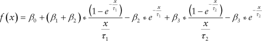
Thus the curve can have two extremums, β₃ determines the size and the form of the second hump, τ₂ specifies the tenor for the second hump.

The advantages of the Svensson method in comparison to OLS and basic N‐S approaches are even better flexibility and better accuracy. However even two humps do not perfectly reflect the market curve. That is why in practice further adjustments were made.

One of them is the adjusted Nelson‐Siegel (adjusted N‐S) approach with a set of seven parameters. The vector of curve's parameters is recalculated after each new bond / new quote is added. The first four parameters (β_s) are responsible for the level of yields on short‐term, middle‐term, and long‐term segments of the yield curve (the shifts up and down), and the remaining three parameters (τ_s) are responsible for convexity / concavity of the appropriate segments.

Such adjustment provides even more advantages: such flexibility that the yield curve by adjusted N‐S approach can have all types of forms: monotonous increasing, or decreasing, convex, U‐form, or S‐form; memory, because the calculation is based on the previous parameters, so additional data doesn't change the form suddenly. This may be especially useful for markets with low liquidity of some bond issues – when on one day bonds are traded, there's a quote and the bond is included in the calculation, but on another day they are not traded, there's no quote and, thus, there's no input for calculation.

The disadvantage of all types of Nelson‐Siegel approaches is their complexity in comparison with the OLS method. As far as one needs to assign initial values to parameters and then apply the “goal seek” function – there's risk that at this moment a mistake is made and further calculations are incorrect.

Nevertheless, one of the Nelson‐Siegel family approaches would be recommended to be used for ALM purposes in the following cases: a) for larger banks with bigger ALM units, equipped with automatic systems; b) on the markets where the curve is supposed to demonstrate several humps on different tenors; c) on bond markets with low liquidity.

To summarise, not all of the existing methods to construct a yield curve can be successfully applied by ALM units. Parametric approaches are most simple in their implementation. The choice between the most “plain vanilla” OLS method and more complicated Nelson‐Siegel family approaches should be done according to the size of the bank and market conditions and peculiarities.

SONIA YIELD CURVE³

An important reference yield curve today is the overnight index swap (OIS) curve. This is similar to the conventional swap curve except it refers to the overnight rate on the floating leg of the swap, compared to the 3‐month or 6‐month rate on the floating leg of a conventional swap.

Prior to the 2008 crash derivative pricing and valuations were based on the simple principle of the time value of money. A breakeven price was calculated such that when all the future implied cash flows were discounted back to today the Net Present Value of all the cash flows was zero. The breakeven price was used for valuations or spread by a bid–offer price to create a trading price. Bid–offers would generally incorporate a counterparty‐dependent mark‐up to cover various costs and a return on capital in a fairly ill‐defined way.

A breakeven price required the construction of a projection curve for the index being referenced, which could be a tenor of Libor, such as 3‐month, for 3‐month Libor swaps or an overnight rate in the case of overnight index swaps. The projection curve would use market observable inputs and various interpolation methodologies to derive market implied future rates used to project the future floating‐rate fixings. In other words:

A conventional swap curve is a projection curve based on the 3‐month (or 6‐month) Libor fix; whereas
An OIS curve is a projection curve based on the overnight rate.

Once the market implied future fixings are known, a discount curve was then used to discount cash flow mismatches in such a way that the breakeven fixed rate gives a result where all the cash flow mismatches have a present value of zero. Historically market practice was to discount cash flows using a Libor discount curve, the assumption being that all cash flow mismatches could be borrowed or reinvested at Libor. It was implicitly assumed that Libor was the risk‐free rate at which these cash flow mismatches could be funded.

Figure 3.2 shows the GBP OIS (known as SONIA) and GBP swap curves as at 13 October 2016. The OIS curve lies below the conventional swap curve because of the term liquidity premium (TLP) difference between the two tenors (the TLP is higher the longer the tenor).

Screenshot illustration of GBP SONIA and GBP Swap curves, 13 October 2016. — **FIGURE 3.2** GBP SONIA and GBP Swap curves, 13 October 2016

*Source*: © Bloomberg LP. Reproduced with permission.

In the case of a collateralised trade transacted under the terms of a CSA, the posting of collateral ensures that the NPV of a trade is always zero net of collateral held or posted. All future funding mismatches are therefore explicitly funded directly by the exchange of collateral and as a result do not require any external funding. The collateral remuneration rate is defined by the CSA and is normally the relevant OIS rate. As it is the relevant OIS rate that becomes the applicable rate for funding cash flow mismatches, market practice has evolved to discount future cash flows using OIS rates when pricing or valuing a collateralised trade, so‐called OIS discounting. It is impossible to determine when this market practice changed but it is generally accepted that when the London Clearing House (which clears derivative transactions) changed to OIS discounting in 2010 it was doing so to reflect best market practice.

Where multiple forms of collateral were permissible under a CSA, market practice evolved to take into account the embedded option for the collateral poster. Pricing assumed that a counterparty would always act rationally and post the cheapest to deliver collateral with the discount curve reflecting the relevant collateral OIS rate, so‐called CTD or CSA discounting. A further enhancement is often used where the collateral is non‐cash such as a government bond, in these instances the discount curve reflects the price at which the bonds can be traded in the repo market. For complex CSAs where collateral was multicurrency, the discount curve is often a multicurrency hybrid curve which reflects that the CTD may change at a future date.

For uncollateralised trades, not only was the use of a Libor rate to discount cash flow mismatches clearly inappropriate given the increase in funding spreads during the 2008 crisis but also, in the absence of collateral, the NPV of an uncollateralised trade represented a potential funding requirement. Pricing for uncollateralised trades now generally contains an upfront adjustment to the price to take into account the expected funding costs of non‐collateralisation referred to as the Funding Valuation Adjustment or FVA. FVA along with a Credit Valuation Adjustment CVA now represent a more rigorously defined part of the bid–offer price adjustment.

Collateral posted at the LCH has no optionality allowed – it must be in cash and in the currency of the transaction. Hence the swap screen price now reflects the price for a cleared swap at LCH. Because the collateral is unambiguous (cash in the currency of the trade) remunerated at the relevant OIS, so the discount / funding rate is always known and is not counterparty dependent. Anything other than a LCH cleared trade means the swap price is different to take into account the impact of the type of collateral. This is an important point: observable swap rates are for LCH cleared trades only.

CONCLUSION

The yield curve is the best snapshot of the state of the financial markets. It is not the sole driver of customer prices in banking, but it is the most influential. Hence it is important that all practitioners understand the behaviour of the curve and how to analyse and interpret it. Being aware of the relationship between spot rates, forward rates, and yield to maturity is also important. Ultimately, there should be no short‐cuts when it comes to understanding the yield curve.

APPENDIX 3.A: ALCO Submission Paper

SELECTED BIBLIOGRAPHY AND REFERENCES

Choudhry, M. (2012), The Principles of Banking, Wiley.
Ferstl, R., Hayden, J., Zero‐Coupon Yield Curve Estimation with the Package termstrc. https://r‐forge.r‐project.org/scm/viewvc.php/*checkout*/pkg/doc/termstrc.pdf?revision=253&root=termstrc&pathrev=253.
Guidelines on Liquidity Cost Benefit Allocation, CEBS, October 2010.
Klein, S. and van Deventer, D. (2009), Yield Curve Smoothing: Nelson‐Siegel versus Spline Technologies, Part 1, Kamakura Corporation Honolulu, 21 July 2009.
Nelson, Ch. and Siegel, A. “Parsimonious Modeling of Yield Curves”, The Journal of Business, Vol. 60, No. 4, October 1987, pp. 473–489.
Principles for Sound Liquidity Risk Management and Supervision. BIS, September 2008.
Zero‐coupon yield curves: technical documentation, BIS Papers, No. 25, Bank for International Settlements, October 2005.

NOTES

..................Content has been hidden....................

You can't read the all page of ebook, please click here login for view all page.

Par yeields	0.05	Df	0.952381
	0.0525		0.9026128
	0.0575		0.8447639	Working	0.1066621
					0.8933379
					1.0575

Table of Contents for CHAPTER 3: The Yield Curve

Create new playlist

Sign In

Sign Up

CONSTRUCTING THE BANK'S INTERNAL YIELD CURVE1

MARKET APPROACH FOR FTP CURVE CONSTRUCTION

APPLICATION OF ORDINARY LEAST SQUARES METHOD AND NELSON‐SIEGEL FAMILY APPROACHES

SONIA YIELD CURVE3

CONCLUSION

APPENDIX 3.A: ALCO Submission Paper

SELECTED BIBLIOGRAPHY AND REFERENCES

NOTES

Table of Contents for
CHAPTER 3: The Yield Curve

CONSTRUCTING THE BANK'S INTERNAL YIELD CURVE¹

SONIA YIELD CURVE³