“The spread of secondary and tertiary education has created a large population of people, often with well‐developed literary and scholarly tastes, who have been educated far beyond their capacity to undertake analytical thought.”
—Peter Medawar, quoted in Richard Dawkins,The Greatest Show on Earth: The Evidence for Evolution, Bantam Press, 2009.
Reiterating our “95–5” rule from Chapter 1, most customer finance requirements – whether long or short of cash – can be met with essentially plain vanilla products. That said, some financial market derivatives have made a positive contribution to society; a good example of this would be the humble interest‐rate swap, without which banks in many countries would not be able to offer fixed‐rate residential mortgages or corporate loans to their customers.
This illustrates the principal reason why derivative instruments are “popular” – they enable an institution to hedge risk exposure. An inability to hedge exposure is the main impediment to a bank offering a customer a desired product such as a fixed‐rate loan. So in this chapter we present previous book extracts that are pertinent to an understanding of the main derivative instruments and the main hedging applications that such products are used for.
The new material in the chapter includes an up‐to‐date discussion on using the asset swap measure to ascertain bond relative value. We also consider the impact of the 2008 crash on the hitherto “standard” pricing principles used for valuing interest‐rate swaps. Swaps have been a collateralised market for some years now, and the previous approach of using solely Libor as the driver of the swap discount factor has had to be modified. The approach described here is important general knowledge for all banks using derivatives in any capacity. Finally, we provide a brief introduction to hedge accounting, again a topic of importance to banks using derivatives.
This extract from Bank Asset and Liability Management (2007)
This extract from Fixed Income Markets, Second Edition (2014)
This extract from The Futures Bond Basis, Second Edition (2006)
This extract from The Credit Default Swap Basis (2006)
ASSET SWAPS AND RELATIVE VALUE
This section can be found in the companion website, in the folder for Chapter 2. Please see Chapter 20 for more details.
This extract from Fixed Income Securities and Derivatives Handbook, Second Edition (2010)
POST‐2008 CRASH SWAP DISCOUNTING AND VALUATION PRINCIPLES1
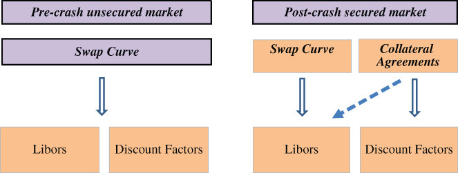
Interest‐rate swaps (IRS) were introduced in the earlier extracts. This section looks at the impact on the swap market of the 2008 bank crash, specifically with respect to pricing and valuation. A large proportion of swaps are now settled via a centralised clearing counterparty (CCP); before that the swap market had become essentially a fully secured market in any case, at least between bank counterparties. The operation of this entailed the mark‐to‐market (MTM) of the swap being passed between the two bilateral counterparties as collateral under the auspices of the credit support annexe (CSA) of the standard ISDA derivatives agreement. Under a CSA, the party that is offside on the swap value (negative MTM) will post collateral to the counterparty equivalent to this MTM value. There is considerable optionality availability in a CSA, which is a legal agreement negotiated between the two parties but if we assume a “gold standard” CSA, which describes (among other things):
Daily margin, equal to end‐of‐day MTM;
Margin in the form of cash, in the currency of the IRS;
No “threshold” amount, so whatever the MTM value the posting takes place at end of day
then this makes the following discussion simpler.
Basic Terms
Herewith some swap basics to ensure everyone is familiar with the key features:
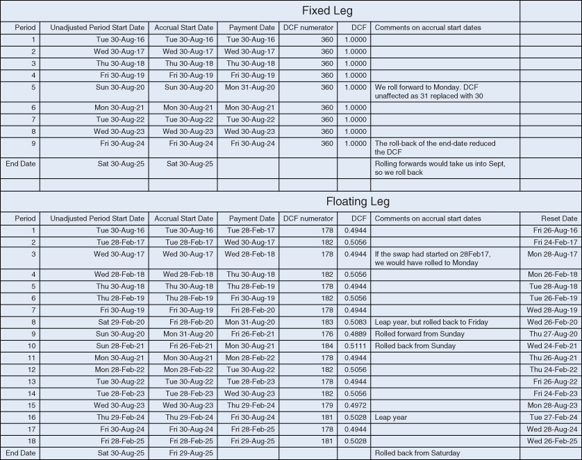
Example definition of an IRS
Notional: 10m EUR
Start Date: 30th August 2016
End Date (Tenor): 30th August 2021 (5 years)
Frequency of payments: Annual fixed, Semi‐annual floating
Fixed Leg accruals: Unadjusted
Floating leg date rolling convention: Modified following (MF)
Floating leg business day calendar for accruals: “Target”
Business day calendar for payments: “Target” for both legs
Business day calendar for resets (floating leg): “Target”
Day count conventions: A/360 floating, 30U/360 fixed
Fixed rate: 1%
Reference for floating rate: 6 month Euribor, reset two days in advance
A “par” swap is defined as a swap with zero mark‐to‐market (MTM). The fixed rate on a par swap can be interpreted as the (discounted) average forward rate over the life of the swap (Figure 2.1).
The CSA is a bilateral agreement governing the collateral posting process. Its most important features describe:
What instruments can be posted as collateral, or if this can be only cash;
The interest rate to be paid on collateral;
Minimum thresholds;
Minimum transfer amounts (MTA).
In theory, a CSA in place removes all credit risk between the two counterparties. (Except an operational risk, known as margin period of risk, arising out of the fact that the MTM value at close of business yesterday may be different the next day when the bank that has posted collateral defaults and the collateral process is finalised so that the non‐defaulting party now has legal ownership of the collateral. This period is accepted to be about 10 days.) A CSA may require, depending on the credit quality of the counterparty, an initial amount (IA) of margin, a standing value, to be posted by one party to the other. Note that CCPs require IA amounts from all their members.
The CSA sets the risk‐free rate for all transactions between the two counterparties; the “CSA rate” is typically the OIS overnight rate in that currency (OIS USD, SONIA for GBP, and EONIA for EUR)
CSAs introduced additional complexity to the swap market because of the optionality that is inherent in them, although the market generally speaks of a “gold standard” CSA with standard terms. For market‐makers in swaps (dealers), issues arise because some swaps on their book will be under a gold standard CSA, others under non‐standard CSAs and some will be uncollateralised.
CCP
The CCP is the central clearing counterparty. They include for example the London Clearing House (LCH) and the Chicago Mercantile Exchange (CME). Virtually all inter‐bank swaps trade through CCPs. The CCP sets the collateral rate, usually the OIS rate in the swap's payment currency. They also charge risk‐based IAs to all members, as we noted above.
Day Count Conventions (Accrual/Payment basis)
Applied to the accrual dates to calculate the weighting of each payment, also known as the Day Count Fraction (DCF) or Accrual Factor. The principal ones are:
Actual/x (Act/x, A/x), where x=360 or 365 most commonly;
(d2 – d1)/x, where di are the accrual start and end dates;
Number of calendar days in the accrual period, divided by the number of days assumed to be in a year, either 360 or 365;
If D2 is 31 and D1 is 30 or 31, then change D2 to 30.
In some cases a convention is denoted as “U”: unadjusted. This is often used with 30/360 to give almost all periods equal weighting.
Determination of the Main (L)ibor Rates
Euribor (Euro Interbank Offered Rate) This is set by a panel of 24 banks, determined by the European Banking Federation, that have the highest volume of business in the euro zone money markets. Each bank submits its rate: the top and bottom 15% are eliminated, and the remaining quotes are averaged. Results are published at 11am CET. In theory, Euribor represents the rate at which these banks lend money to each other on unsecured loans. The tenors that are quoted are overnight, 1‐week, 2‐week, 1‐, 2‐, 3‐, 6‐, 9‐ and 12‐month rates.
Note that the reference swaps are very liquid but that not every bank is able to borrow unsecured in the inter‐bank market at Libor‐flat. Some banks, with lower credit ratings, will pay a spread over the relevant term Libor rate for borrowing unsecured, where they have borrowing lines with other banks (again, not every bank has such access).
Alternative Fixing Source: Overnight Indexed Swaps (OIS)
The OIS rate is the average of unsecured overnight lending rates between banks. It is closer to the risk‐free, but of course still contains some credit and liquidity risk. (We assume the risk‐free rate to be the US T‐bill rate.)
The USD OIS swap references the Federal Funds Effective Rate, whereas other currencies references overnight Libor or Euribor. The common currencies are:
GBP Over‐Night Indexed Average (SONIA);
EUR Over‐Night Indexed Average (EONIA);
JPY Over‐Night Indexed Average (TONAR).
The mechanics of OIS swaps are covered elsewhere in this chapter, in the extract from the book Bank Asset Liability Management.
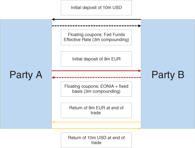
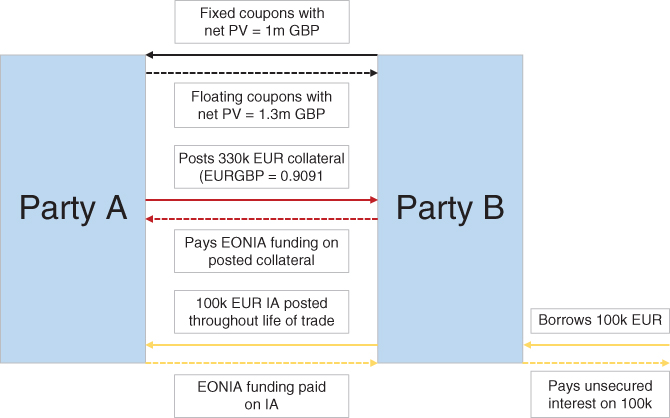
Example Structure Diagrams
Figures 2.2 and 2.3 show a cross‐currency basis swap example and a swap transacted under a CSA agreement.
The discount factor represents the present value of a £1 (or $1) unit cash flow paid at a specified future date. The rate is the expected cost of funding the cash flow continuously overnight until maturity.
At the inception of the bilateral OTC swaps market, due to the definition of a swap, banks were already using Libor (or Euribor) in forecasting future cash flows. At that time, swaps were uncollateralised, and the valuation process assumed that all banks could fund at Libor‐flat; hence Libor‐flat would be the rate used to fund swap cash flows. Hence, future cash flows associated with a swap were discounted at the same rate where banks were assumed to fund themselves (Libor‐flat). Of course, in the lead‐up to the 2008 crash and subsequently, many banks were not able to fund themselves at Libor‐flat and instead funded at Libor+spread, hence the origination of the funding value adjustment (FVA), to reflect the actual funding cost of banks. This is very material in a collateralised swap market, as we have now, as banks have to fund the collateral requirement.
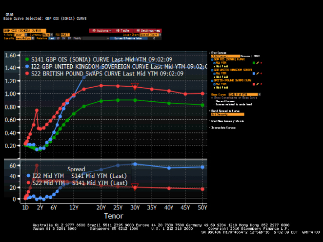
Discounting affects the par swap rate. This is not necessarily relevant if every swap transacted by a bank is collateralised under a CSA (although it may be), but given that a swap is funded (in terms of collateral) at the OIS rate, but the floating‐rate re‐fix references the Libor rate showing the UK sovereign curve, GBP vanilla swaps curve, and the SONIA curve) there may be valuation issues especially for longer‐dated swaps. (The Libor and OIS yield curves are different, see Figure 2.4 which is a Bloomberg screen as at 13 September 2016.) To agree the MTM for collateral posting, bilateral swaps would have to agree the discounting curve in order to agree the collateral margin. CCP‐cleared swaps will all value to the CCP convention.
FIGURE 2.4 GBP Swaps and OIS curves, September 2016
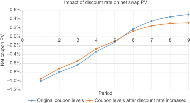
Note, typically yield curves are upward‐sloping. A high discount rate reduces the value of longer‐dated cash flows more, and this reduces their weighting in the total PV, causing the par swap rate to fall. If one discounts “wrongly” (such as with Libor), one will misprice steep yield curves and out‐of‐money swaps. A stylised illustration of this effect is shown at Figure 2.5.
Uncollateralised swaps are discounted at a rate that depends on the credit‐risk of the two counterparties. Bilaterally collateralised swaps are discounted at the CSA rate, and swaps cleared through the CCP are collateralised at a standard OIS rate.
Independent Amounts (IAs) can be charged by banks facing customers. CCPs charge banks IAs which the bank will fund at its specific funding rate.
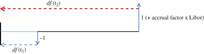
The relationship between Libor and discount factors is illustrated using Figure 2.6 and expressions below. This shows in effect a dual‐purpose Libor; first a forecasting rate for future cash flows and second a measure for how to discount cash flows.
FIGURE 2.6 Relationship between Libor and discount factors
When pricing a swap on Day 1, we assume that par swap rates have zero net present value (NPV), hence a single swap curve is sufficient both to forecast Libors and determine discount factors. The basic description for this is given in Appendix 2.1.
How Does Collateral Impact the Discount Rate?
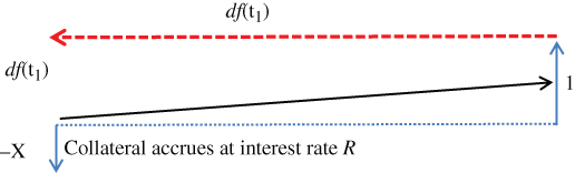
Consider the collateralised deal shown at Figure 2.7.
FIGURE 2.7 How collateral impacts the discount rate
At t0 we lend EUR X, to receive EUR 1 at t1. As collateral we immediately receive the mutually agreed NPV which is df(t1) hence it is analogous to a secured loan. Since both parties agree this is the contract NPV, the following must hold:
This implies our net cash position is equal to zero: our portfolio is in balance and there is no need to fund via the money market.
On the collateral cash we have specified an interest rate payable of R, which gives an amount of:
where α is the day‐count accrual factor and the earlier expression is for the notional amount X.
At t1 two cash flows take place.
We receive EUR 1 and we pay the collateral amount back plus interest. Assuming a no‐arbitrage environment these cash flows must be identical and so the following will hold:
It is the interest R on the collateral that determines the discount factor.
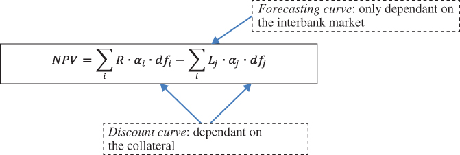
Moving to swap valuation, the collateral cash is the swap MTM, so since the collateral rate (generally OIS, SONIA, or EONIA for USD, GBP, and EUR respectively) determines the discounting curve, we need to use two curves to value the swap book. This is shown at Figure 2.8.
FIGURE 2.8 Separating the forecasting and discounting curve
So when valuing a collateralised swap, we consider both curves. Inter‐bank swap quotes are based on the CSA (or CCP as appropriate) collateral funding rate, generally OIS. The swap curve and the overnight curve forecast Libors, so the forecasting curve is known. The same Libor forecast is used for all secured swaps, irrespective of the actual form of the collateral. Hence, the NPV of a swap is calculated with a discounting curve that is based on the actual posted collateral. As the posted collateral is designed to reflect the swap MTM, the logic is clear.
Figure 2.9 summarises this principle, where the expressions used are again:
In practice, banks will use an FVA adjustment to account for their own funding rate (where they are borrowing to post cash collateral) in the swap valuation.
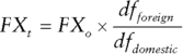
Cross‐Currency Swaps With respect to cross‐currency swaps, in the lead‐up to the Lehman default and subsequently, a cross‐currency basis swap appeared, due to supply/demand, credit, and liquidity. The market had assumed that it could always discount using 3m USD Libor, cross‐currency swapped. For example, euro cash flows would be discounted at 3m Euribor + XCCY basis spread. Post‐Lehman's, the Libor‐OIS spreads blew up, and this assumption failed. (Even pre‐Lehman it was a poor assumption.) At the present time, we know the single currency OIS rates from OIS swaps. The discount factor depends on the trade currency and the collateral type (or lack thereof). Cross‐currency swaps also trade against OIS. The basis spread allows us to calculate our CSA discount factors.
We can use the ratio of two discount rates to calculate the forward FX rate:
A large number of banks around the world employ financial derivative instruments when hedging interest‐rate and FX risk exposure on the balance sheet. Derivatives are treated as “trading book” products requiring daily marking‐to‐market revaluation. This generates a P&L impact, which can be addressed by the application of the “hedge accounting” concept.
In this section, we consider the ALM implications of hedge accounting, as well as the capital reporting issues associated with the trading book.
A banking book exposes a bank to interest rate and credit risks. A banking book may also comprise financial instruments denominated in foreign currency, equities and commodities, exposing the bank to foreign exchange (FX), equity, and commodity risks.
These risks are commonly hedged with derivatives. The international accounting standard that sets out the guidelines to recognise derivatives is IFRS 9. In July 2014, the International Accounting Standards Board (IASB) issued IFRS 9 Financial Instruments, which replaced IAS 39 Financial Instruments: Recognition and Measurement, and included requirements for classification and measurement of financial assets and liabilities, impairment of financial assets, and hedge accounting. IFRS 9 came into force on 2 January 2018.
Derivatives are recognised initially, and are subsequently measured, at fair value, regardless of whether they are held for trading or hedging purposes. Fair values of derivatives are obtained either from quoted market prices or by using valuation techniques. Derivatives are classified as assets when their fair value is positive or as liabilities when their fair value is negative.
Gains and losses from changes in the fair value of derivatives that do not qualify for hedge accounting are reported in “net trading income” (i.e., not reported in “net interest income”).
Accounting Approach
In a hedge accounting relationship there are two elements: the hedged item and the hedging instrument.
The hedged item is the item that exposes the entity to a market risk(s). It is the element that is designated as being hedged;
The hedging instrument is the element that hedges the risk(s) to which the hedged item is exposed. Most of the time, the hedging instrument is a derivative.
For example, a bank hedging an issued variable rate bond with a pay‐fixed receive‐floating interest‐rate swap and applying hedge accounting would designate the bond as the hedged item and the swap as the hedging instrument.
Hedge accounting is a technique that modifies the normal basis for recognising gains and losses (or revenues and expenses) associated with a hedged item or a hedging instrument to enable gains and losses on the hedging instrument to be recognised in profit or loss in the same period as offsetting losses and gains on the hedged item.
The application of hedge accounting is voluntary. In other words, were a bank to hedge a specific market risk with a derivative, it is not obliged to apply hedge accounting. However, were a bank willing to apply hedge accounting, it may not be able to do so. To qualify for hedge accounting, these are the three requirements that a hedging relationship must meet:
The hedging relationship consists only of eligible hedging instruments and eligible hedged items;
At the inception of the hedging relationship there is formal designation and documentation of the hedging relationship and the entity's risk management objective and strategy for undertaking the hedge. That documentation shall include identification of the hedging instrument, the hedged item, the nature of the risk being hedged and how the entity will assess whether the hedging relationship meets the hedge effectiveness requirements (including its analysis of the sources of hedge ineffectiveness and how it determines the hedge ratio); and
The hedging relationship meets all the three hedge effectiveness requirements.
The three hedge effectiveness requirements are the following:
There is an economic relationship between the hedged item and the hedging instrument;
The effect of credit risk does not dominate the value changes that result from that economic relationship; and
The weightings of the hedged item and the hedging instrument (i.e., the hedge ratio of the hedging relationship) is the same as that resulting from the quantity of the hedged item that the entity actually hedges and the quantity of the hedging instrument that the entity actually uses to hedge that quantity of hedged item. However, that designation shall not reflect an imbalance between the weightings of the hedged item and the hedging instrument that would create hedge ineffectiveness (irrespective of whether recognised or not) that could result in an accounting outcome that would be inconsistent with the purpose of hedge accounting.
Hedge accounting takes three forms under IFRS 9: fair value hedge, cash flow hedge, and net investment hedge.
Fair Value Hedge
A fair value hedge hedges the change in fair value of a recognised asset or liability or firm commitment.
In the case of interest rate risk hedges, a bank enters into fair value hedges, using primarily interest rate swaps and options, in order to protect itself against movements in the fair value of fixed‐rate financial instruments due to movements in market interest rates.
In a fair value hedge, the changes in the fair value of the hedged asset, liability or unrecognised firm commitment, or a portion thereof, attributable to the risk being hedged, are recognised in the profit or loss statement along with changes in the entire fair value of the derivative. When hedging interest rate risk, any interest accrued or paid on both the derivative and the hedged item is reported in “net interest income”, and the unrealised gains and losses from the hedge accounting fair value adjustments are reported in “net trading income” (i.e., not reported in “net interest income”) in profit or loss.
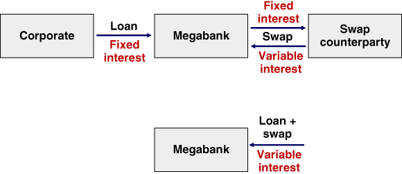
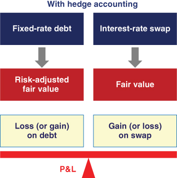
Let us assume that Megabank provided a fixed‐rate loan to a corporate. Because the fair value of the loan was exposed to changes in interest rates (and the corporate credit spread), Megabank decided to enter into a pay‐fixed receive‐floating interest rate swap. The combination of the loan and the swap resembled an origination of a variable‐rate loan, as shown at Figure 2.10.
FIGURE 2.10 Combined interest flows of the loan and the interest rate swap
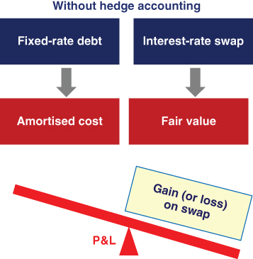
Let us assume that Megabank decided not to apply hedge accounting. In such a case, the interest income stemming from the loan and the swap settlement amounts were recognised in profit or loss. The loan was recognised at amortised cost. In contrast, the swap was recognised at fair value through profit or loss, meaning that the changes in fair value of the swap were recognised in profit or loss. Ignoring the loan interest income and the swap settlement amounts, the hedging strategy added volatility to Megabank's profit or loss statement, as shown at Figure 2.11, although the strategy mitigated Megabank's exposure to interest rates stemming from the loan fair value.
Let us assume instead that the hedging relationship met the requirements for the application of hedge accounting and that Megabank decided to apply hedge accounting. As in the case of no application of hedge accounting, the interest income stemming from the loan and the swap settlement amounts were recognised in profit or loss. As in the case of no application of hedge accounting, the changes in fair value of the swap were recognised in profit or loss. Through the application of fair value hedge, the loan was fair valued and changes in its fair value due to changes in interest rates were recognised in profit or loss. If the hedge was well constructed, the changes in fair value of the swap would be offset by the changes in fair value of the loan (for changes in interest rates) and, therefore, the hedge would not add volatility in profit or loss, as shown at Figure 2.12 (ignoring the loan interest income and the swap settlement amounts). Therefore, the application of hedge accounting changed the recognition of the loan to align it with the recognition of the swap.
FIGURE 2.12 Application of fair value hedge accounting
Cash Flow Hedge
These are hedges set up to address variability in expected future cash flows that are attributable to a recognised specific asset or liability, or to a future expected transaction.
In the case of interest‐rate risk hedges, a bank enters into cash flow hedges, using primarily interest rate swaps and options, futures, and cross‐currency swaps, in order to protect itself against exposures to variability, due to movements in market interest rates, in future interest cash flows on banking book assets, and liabilities which bear interest at variable rates or which are expected to be re‐funded or reinvested in the future.
In a cash flow hedge, there is no change to the accounting for the hedged item and the derivative is carried at fair value, with changes in value reported initially in other comprehensive income to the extent the hedge is effective. These amounts initially recorded in other comprehensive income are subsequently reclassified into the profit or loss statement in the same periods during which the forecast transaction affects the profit or loss statement. (There is an exception for hedges of equities recognised at fair value though other comprehensive income.) For hedges of interest rate risk, the amounts are amortised into “net interest income” at the same time as the interest is accrued on the hedged transaction.
Hedge ineffectiveness is recorded in “net trading income” in profit or loss and is measured as changes in the excess (if any) in the absolute cumulative change in fair value of the actual hedging derivative over the absolute cumulative change in the fair value of the hypothetically perfect hedge.
Net Investment Hedge
A net investment hedge is a hedge of the net investment in a foreign operation. In other words, it is the hedge of the translation adjustments resulting from translating the functional currency financial statements of the foreign operation into the presentation currency of the parent entity. Imagine that Megabank was a British bank with the GBP as its presentation currency and that it controlled a French bank which reported in EUR. The financial statements of the French subsidiary will be disclosed in EUR and translated into GBP when the group prepares its consolidated financial statements. As a result, Megabank would be exposed to a potential depreciation of the EUR against the GBP. Megabank may hedge such an exposure by entering into, for example, a GBP/EUR FX forward in which the bank receives a fixed amount of GBP in exchange for a fixed amount of EUR.
In a net investment hedge, the portion of the change in fair value of the derivative due to changes in the spot (or forward) foreign exchange rate is recorded as a foreign currency translation adjustment in other comprehensive income to the extent the hedge is effective; the remainder is recorded in “net trading income” in profit or loss.
Changes in fair value of the hedging instrument relating to the effective portion of the hedge are subsequently recognised in profit or loss on disposal of the foreign operations.
APPENDIX 2.A: The Par Asset Swap Spread
We assume we have constructed a market curve of Libor discount factors where Df(t) is the price today of $1 to be paid at time t. From the perspective of the asset swap seller, it sells the bond for par plus accrued interest. The net up‐front payment has a value 100 – P where P is the market price of the bond. If we assume both parties to the swap are inter‐bank credit quality, we can price the cash flows off the Libor curve.
For the calculation we cancel out the principal payments of par at maturity. We assume that cash flows are annual and take place on the same coupon dates. The breakeven asset swap spread A is calculated by setting the present value of all cash flows equal to zero. From the perspective of the asset swap seller, the present value is
(2A.1)
There is a 100 – P upfront payment to purchase the asset in return for par. For the interest rate swap we have
(2A.2)
for the fixed payments and
(2A.3)
for the floating payments, where C equals the bond annual coupon, Li is the Libor rate set at time ti ‐ l and paid at time ti, and Di is the accrual factor in the corresponding basis (day‐count adjustment). We then solve for the asset swap spread A.
SELECTED BIBLIOGRAPHY AND REFERENCES
Choudhry, M., “An alternative bond relative value measure: determining a fair value of the swap spread using Libor and GC repo rates”, Journal of Asset Management 7 (1), June 2005, pp. 17–21.
Gale, G., “Using and trading asset‐swaps: interest rate strategy”, Morgan Stanley Fixed Income Research, May 2006.
O'Kane, D., Sen, S., “Credit spreads explained”, Journal of Credit Risk 1 (2), Spring 2005, pp. 61–78.