
Chapter 5
Building PivotTable Formulas
In This Chapter
![]() Adding another standard calculation
Adding another standard calculation
![]() Creating custom calculations
Creating custom calculations
![]() Using calculated fields and items
Using calculated fields and items
![]() Retrieving data from a pivot table
Retrieving data from a pivot table
Most of the techniques that I discuss in this chapter aren't things that you need to do very often. Most frequently, the cross-tabulated data that appears in a pivot table after you run the PivotTable Wizard are almost exactly what you need. And if not, a little bit of fiddling around with the item buttons gets the information into the perfect arrangement for your needs. (For more on the PivotTable Wizard, read through Chapter 4.)
On occasion, however, you'll find that you need to either grab information from a pivot table so that you can use it someplace else or that you need to hard-code calculations and add them to a pivot table. In these special cases, the techniques that I describe in this chapter might save you much wailing and gnashing of teeth.
Adding Another Standard Calculation
Take a look at the pivot table shown in Figure 5-1. This pivot table shows coffee sales by state for an imaginary business that you can pretend that you own and operate. The data item calculated in this pivot table is sales. Sometimes, sales might be the only calculation that you want made. But what if you also want to calculate average sales by product and state in this pivot table?
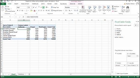
Figure 5-1: Add standard calculations to basic pivot tables for more complex data analysis.
Note: You can find this Excel Data List of Coffees with Pivottable Custom Calculations Workbook, available in the Zip file of sample Excel workbooks related to this book, at the companion site for this book. (See this book's Introduction for more on how to access the companion site.) You might want to download this list in order to follow along with the discussion here.
To do this, right-click the pivot table and choose Value Field Settings from the shortcut menu that appears. Then, when Excel displays the Value Field Settings dialog box, as shown in Figure 5-2, select Average from the Summarize Value Field By list box.
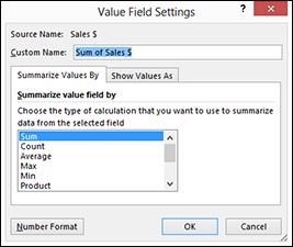
Figure 5-2: Replace calculations here.
Now assume, however, that you don't want to replace the data item that sums sales. Assume instead that you want to add average sales data to the worksheet. In other words, you want your pivot table to show both total sales and average sales.
Note: If you want to follow along with this discussion, start over from scratch with a fresh copy of the worksheet shown in Figure 5-1.
To add a second summary calculation, or standard calculation, to your pivot table, drag the data item from the PivotTable Field list box to the Σ Values box. Figure 5-3 shows how the roast coffee product sales by state pivot table looks after you drag the sales data item to the pivot table a second time. You may also need to drag the Σ Values entry from the Columns box to the Row box. (See the Columns and Rows boxes at the bottom of the PivotTable Field List.)
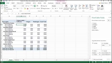
Figure 5-3: Add a second standard summary calculation to a pivot table.
After you add a second summary calculation — in Figure 5-3, this shows as the Sum of Sales $2 data item — right-click that data item, choose Value Field Settings from the shortcut menu that appears, and use the Value Field Settings dialog box to name the new average calculation and specify that the average calculation should be made. In Figure 5-4, you can see how the Value Field Settings dialog box looks when you make these changes for the pivot table shown in Figure 5-3.
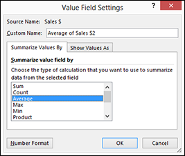
Figure 5-4: Add a second standard calculation to a pivot table.
See Figure 5-5 for the new pivot table. This pivot table now shows two calculations: the sum of sales for a coffee product in a particular state and the average sale. For example, in cell B6, you can see that sales for the Best Blend of the Arabia coffee are $6,186 in California. And in cell B7, the pivot table shows that the average sale of the Best Blend of Arabia coffee in California is $476.
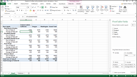
Figure 5-5: A pivot table with two standard calculations.
 If you can add information to your pivot table by using a standard calculation, that's the approach you want to take. Using standard calculations is the easiest way to calculate information, or add formulas, to your pivot tables.
Creating Custom Calculations
Excel pivot tables provide a feature called Custom Calculations. Custom Calculations enable you to add many semi-standard calculations to a pivot table. By using Custom Calculations, for example, you can calculate the difference between two pivot table cells, percentages, and percentage differences.
To illustrate how custom calculations work in a pivot table, take a look at Figure 5-6. This pivot table shows coffee product sales by month for the imaginary business that you own and operate. Suppose, however, that you want to add a calculated value to this pivot table that shows the difference between two months' sales. You may do this so that you easily see large changes between two months' sales. Perhaps this data can help you identify new problems or important opportunities.
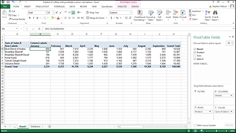
Figure 5-6: Use custom calculations to compare pivot table data.
To add a custom calculation to a pivot table, you need to complete two tasks: You need to add another standard calculation to the pivot table, and you need to then customize that standard calculation to show one of the custom calculations listed in Table 5-1.
Table 5-1 Custom Calculation Options for Pivot Tables
|
Calculation |
Description |
|
Normal |
You don’t want a custom calculation. |
|
Difference From |
This is the difference between two pivot table cell values; for example, the difference between this month's and last month's value. |
|
% of |
This is the percentage that a pivot table cell value represents compared with a base value. |
|
% Difference From |
This is the percentage difference between two pivot table cell values; for example, the percentage difference between this month’s and last month’s value. |
|
Running Total In |
This shows cumulative or running totals of pivot table cell values; for example, cumulative year-to-date sales or expenses. |
|
% of Row |
This is the percent that a pivot table cell value represents compared with the total of the row values. |
|
% of Column |
This is the percent that a pivot table cell value represents compared with the total of the column values. |
|
% of Total |
This is the pivot table cell value as a percent of the grand total value. |
|
Index |
Kind of complicated, dude. The index custom calculation uses this formula: ((cell value) x (grand total of grand totals)) / ((grand total row) x (grand total column)). |
To add a second standard calculation to the pivot table, add a second data item. For example, in the case of the pivot table shown in Figure 5-6, if you want to calculate the difference in sales from one month to another, you need to drag a second sales data item from the field list to the pivot table. Figure 5-7 shows how your pivot table looks after you make this change.
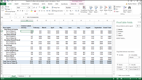
Figure 5-7: Add a second standard calculation and then customize it.
After you add a second standard calculation to the pivot table, you must customize it by telling Excel that you want to turn the standard calculation into a custom calculation. To do so, follow these steps:
- Click the new standard calculation field from the Σ Values box, and then choose Value Field Settings from the shortcut menu that appears.
- When Excel displays the Value Field Settings dialog box, as shown in Figure 5-8, click the Show Values As tab.
The Show Values As tab provides three additional boxes: Show Values As, Base Field, and Base Item.
The Base Field and Base Item list box options that Excel offers depend on which type of custom calculation you’re making.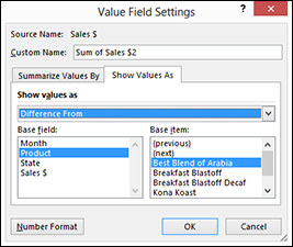
Figure 5-8: Customize a standard calculation here.
- Select a custom calculation by clicking the down-arrow at the right side of the Show Values As list box and then selecting one of the custom calculations available in that drop-down list.
For example, to calculate the difference between two pivot table cells, select the Difference From entry. Refer to Table 5-1 for explanation of the possible choices.
- Instruct Excel about how to make the custom calculation.
After you choose the custom calculation that you want Excel to make in the pivot table, you make choices from the Base Field and Base Item list boxes to specify how Excel should make the calculation. For example, to calculate the difference in sales between the current month and the previous month, select Month from the Base Field list box and Previous from the Base Item list box. Figure 5-9 shows how this custom calculation gets defined.
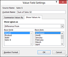
Figure 5-9: Define a custom calculation here.
- Appropriately name the new custom calculation in the Custom Name text box of the Data Field Settings dialog box.
For example, to calculate the change between two pivot table cells and the cells supply monthly sales, you may name the custom calculation Change in Sales from Previous Month. Or, more likely, you may name the custom calculation Mthly Change.
- Click OK.
Excel adds the new custom calculation to your pivot table, as shown in Figure 5-10.
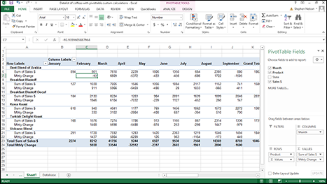
Figure 5-10: Your pivot table now shows a custom calculation.
Using Calculated Fields and Items
Excel supplies one other opportunity for calculating values inside a pivot table. You can also add calculated fields and items to a table. With these calculated fields and items, you can put just about any type of formula into a pivot table. But, alas, you need to go to slightly more work to create calculated fields and items.
Adding a calculated field
Adding a calculated field enables you to insert a new row or column into a pivot table and then fill the new row or column with a formula. For example, if you refer to the pivot table shown in Figure 5-10, you see that it reports on sales both by product and month. What if you want to add the commissions expense that you incurred on these sales?
Suppose for the sake of illustration that your network of independent sales representatives earns a 25 percent commission on coffee sales. This commission expense doesn't appear in the data list, so you can't retrieve the information from that source. However, because you know how to calculate the commissions expense, you can easily add the commissions expense to the pivot table by using a calculated field.
To add a calculated field to a pivot table, take the following steps:
- Identify the pivot table by clicking any cell in that pivot table.
- Tell Excel that you want to add a calculated field.
Click the Analyze ribbon’s Fields, Items & Sets command, and then choose Calculated Field from the Formulas menu. Excel displays the Insert Calculated Field dialog box, as shown in Figure 5-11.
 In Excel 2007and Excel 2010, you choose the PivotTable Tools Option tab’s Formulas command and then choose Calculated Field from the Formulas menu.
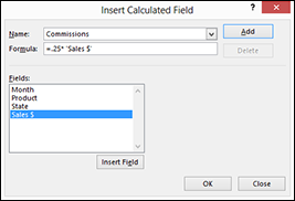
Figure 5-11: Add a calculated field here.
- In the Name text box, name the new row or column that you want to show the calculated field.
For example, if you want to add a row that shows commissions expense, you might name the new field Commissions.
- Write the formula in the Formula text box.
Calculated field formulas work the same way as formulas for regular cells:
- Begin the formula by typing the equal (=) sign.
- Enter the operator and operands that make up the formula.
If you want to calculate commissions and commissions equal 25 percent of sales, enter =.25*.
- The Fields box lists all the possible fields that can be included in your formula. To include a choice from the Fields list, click the Sales $ item in the Fields list box and then click the Insert Field button.
See in Figure 5-11 how the Insert Calculated Field dialog box looks after you create a calculated field to show a 25 percent commissions expense.
- Click OK.
Excel adds the calculated field to your pivot table. Figure 5-12 shows the pivot table with coffee product sales with the Commissions calculated field now appearing.
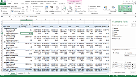
Figure 5-12: A pivot table with a calculated field.
After you insert a calculated field, Excel adds the calculated field to the PivotTable field list. You can then pretty much work with the calculated item in the same way that you work with traditional items.
Adding a calculated item
You can also add calculated items to a pivot table. Now, frankly, adding a calculated item usually doesn't make any sense. If, for your pivot table, you have retrieved data from a complete, rich Excel list or from some database, creating data by calculating item amounts is more than a little goofy. However, in the spirit of fair play and good fun, here I create a scenario where you might need to do this using the sales of roast coffee products by months.
Assume that your Excel list omits an important product item. Suppose that you have another roast coffee product called Volcano Blend Decaf. And even though this product item information doesn't appear in the source Excel list, you can calculate this product item's information by using a simple formula.
Also assume that sales of the Volcano Blend Decaf product equal exactly and always 25 percent of the Volcano Blend product. In other words, even if you don't know or don't have Volcano Blend Decaf product item information available in the underlying Excel data list, it doesn't really matter. If you have information about the Volcano Blend product, you can calculate the Volcano Blend Decaf product item information.
Here are the steps that you take to add a calculated item for Volcano Blend Decaf to the Roast Coffee Products pivot table shown in earlier figures in this chapter:
- Select the Product button by simply clicking the Row Labels button in the pivot table.
- Tell Excel that you want to add a calculated item to the pivot table.
Click the Analyze ribbon’s Fields, Items & Settings command and then choose Calculated Items from the submenu that appears. Excel displays the Insert Calculated Item in “Product” dialog box, as shown in Figure 5-13.
In Excel 2007 or Excel 2010, click the PivotTable Tools Options tab’s Formulas command and then choose Calculated Items from the Formulas submenu that appears.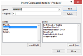
Figure 5-13: Insert a calculated item here.
- Name the new calculated item in the Name text box.
In the example that I set up here, the new calculated item name is Volcano Blend Decaf, so that's what you enter in the Name text box.
- Enter the formula for the calculated item in the Formula text box.
Use the Formula text box to give the formula that calculates the item. In the example here, you can calculate Volcano Blend Decaf sales by multiplying Volcano Blend sales by 25 percent. This formula then is =.25*‘Volcano Blend'.
- To enter this formula into the Formula text box, first type =.25*.
- Then select Volcano Blend from the Items list box and click the Insert Item button.
See Figure 5-14 for how the Insert Calculated Item in “Product” dialog box looks after you name and supply the calculated item formula.
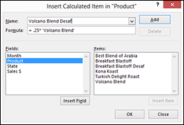
Figure 5-14: The Insert Calculated Item dialog box after you do your dirty work.
- Add the calculated item.
After you name and supply the formula for the calculated item, click OK. Excel adds the calculated item to the pivot table. Figure 5-15 shows the pivot table of roast coffee product sales by month with the new calculated item, Volcano Blend Decaf. This isn't an item that comes directly from the Excel data list, as you can glean from the preceding discussion. This data item is calculated based on other data items: in this case, based on the Volcano Blend data item.

Figure 5-15: The new pivot table with the inserted calculated item.
Removing calculated fields and items
You can easily remove calculated fields and items from the pivot table.
To remove a calculated field, click a cell in the pivot table. Then click the Analyze tab’s Fields, Items & Sets command and choose Calculated Field from the submenu that appears. When Excel displays the Insert Calculated Field dialog box, as shown in Figure 5-16, select the calculated field that you want to remove from the Name list box. Then click the Delete button. Excel removes the calculated field.
In Excel 2007 or Excel 2010, click the PivotTable Tools Options tab’s Formulas command and choose Calculated Field from the Formulas submenu to display the Insert Calculated Field dialog box shown in Figure 5-16.
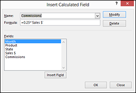
Figure 5-16: Use the Insert Calculated Field dialog box to remove calculated fields from the pivot table.
To remove a calculated item from a pivot table, perform the following steps:
- Click the button of the calculated item that you want to remove.
For example, if you want to remove the Volcano Blend Decaf item from the pivot table shown in Figure 5-15, click the Product button.
- Click the Analyze tab’s Fields, Items 7 Settings button and then click Calculated Item from the menu that appears.
The Insert Calculated Item dialog box appears.
In Excel 2007 or Excel 2010, you click the Options tab’s Formulas button and then choose Calculated Item from the menu in order to display the Insert Calculated Item dialog box. - Select the calculated item from the Name list box that you want to delete.
- Click the Delete button.
- Click OK.
Figure 5-17 shows the Insert Calculated Item in “Product” dialog box as it looks after you select the Volcano Blend Decaf item to delete it.
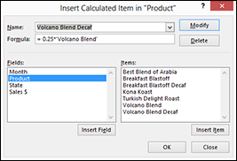
Figure 5-17: Delete unwanted items from the Insert Calculated Item dialog box.
Reviewing calculated field and calculated item formulas
If you click the Analyze tab’s Fields, Items & Settings command and choose List Formulas from the submenu that appears, Excel adds a new sheet to your workbook. This new sheet, as shown in Figure 5-18, identifies any of the calculated field and calculated item formulas that you add to the pivot table.
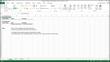
Figure 5-18: The Calculated Field and Calculated Item list of formulas worksheet.
In Excel 2007 or Excel 2010, you click the PivotTable Tools Options tab’s Formulas button and then choose List Formulas from the menu in order to display the new sheet and its list of calculated fields.
For each calculated field or item, Excel reports on the solve order, the field or item name, and the actual formula. If you have only a small number of fields or items, the solve order doesn't really matter. However, if you have many fields and items that need to be computed in a specific order, the Solve Order field becomes relevant. You can pick the order in which fields and items are calculated. The Field and Item columns of the worksheet give a field or item name. The Formula column shows the actual formula.
Reviewing and changing solve order
If you click the Analyze tab’s Fields, Items & Settings command and choose Solve Order from the submenu that appears, Excel displays the Calculated Item Solve Order dialog box, as shown in Figure 5-19. In this dialog box, you tell Excel in what order the calculated item formulas should be solved.
In Excel 2007 or Excel 2010, you click the PivotTable Tools Options tab’s Formulas button and then choose Calculated Item from the menu in order to display the Insert Calculated Item dialog box.
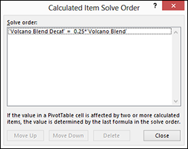
Figure 5-19: Set solve order here.
In many cases, the solve order doesn't matter. But if, for example, you add calculated items for October, November, and December to the Kona Koast coffee product sales pivot table shown earlier in the chapter (refer to Figure 5-6), the solve order might just matter. For example, if the October calculated item formula depends on the previous three months and the same thing is true for November and December, you need to calculate those item values in chronological order. Use the Calculated Item Solve Order dialog box to do this. To use the dialog box, simply click a formula in the Solve Order list box. Click the Move Up and Move Down buttons to put the formula at the correct place in line.
Retrieving Data from a Pivot Table
You can build formulas that retrieve data from a pivot table. Like, I don’t know, say that you want to chart some of the data shown in a pivot table. You can also retrieve an entire pivot table.
Getting all the values in a pivot table
To retrieve all the information in a pivot table, follow these steps:
- Select the pivot table by clicking a cell within it.
- Click the Analyze tab’s Select command and choose Entire PivotTable from the menu that appears.
Excel selects the entire pivot table range.
In Excel 2007 or Excel 2010, click the PivotTable Tools Options tab’s Options command, click Select, and choose Entire Table from the Select submenu that appears. - Copy the pivot table.
You can copy the pivot table the same way that you would copy any other text in Excel. For example, you can click the Home tab’s Copy button or by pressing Ctrl+C. Excel places a copy of your selection onto the Clipboard.
- Select a location for the copied data by clicking there.
- Paste the pivot table into the new range.
You can paste your pivot table data into the new range in the usual ways: by clicking the Paste button on the Home tab or by pressing Ctrl+V. Note, however, that when you paste a pivot table, you get another pivot table. You don't actually get data from the pivot table.
If you want to get just the data and not the pivot table — in other words, you want a range that includes labels and values, not a pivot table with pivot table buttons — you need to use the Paste Special command. (The Paste Special command is available from the menu that appears when you click the down-arrow button beneath the Paste button.) When you choose the Paste Special command, Excel displays the Paste Special dialog box, as shown in Figure 5-20. In the Paste section of this dialog box, select the Values radio button to indicate that you want to paste just a range of simple labels and values and not a pivot table itself. When you click OK, Excel pastes only the labels and values from the pivot table and not the actual pivot table.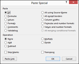
Figure 5-20: Paste information from a pivot table rather than the entire pivot table.
Getting a value from a pivot table
To get a single value from a pivot table using a formula, create a cell reference. For example, suppose that you want to retrieve the value shown in cell C8 in the worksheet shown in Figure 5-21. Further suppose that you want to place this value into cell C15. To do this, click cell C15, type the = sign, click cell C8, and then press Enter. Figure 5-21 shows how your worksheet looks before you press Enter. The formula shows.
As you can see in Figure 5-21, when you retrieve information from an Excel pivot table, the cell reference isn't a simple cell reference as you might expect. Excel uses a special function to retrieve data from a pivot table because Excel knows that you might change the pivot table. Therefore, upon changing the pivot table, Excel needs more information about the cell value or data value that you want than simply its previous cell address.
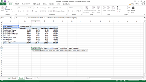
Figure 5-21: How the worksheet looks after you tell Excel you want to place the Kona Koast sales for Oregon value into cell C15.
Look a little more closely at the GET pivot table formula shown in Figure 5-21. The actual formula is
=GETPIVOTDATA("Sales$",$A$3,"Product","KonaKoast","State",
"Oregon")
The easiest way to understand the GETPIVOTDATA function arguments is by using the Insert Function command. To show you how this works, assume that you enter a GETPIVOTDATA function formula into cell C15. This is the formula that Figure 5-21 shows. If you then click cell C15 and choose the Formulas tab’s Function Wizard command, Excel displays the Function Arguments dialog box, as shown in Figure 5-22. The Function Arguments dialog box, as you might already know if you’re familiar with Excel functions, enables you to add or change arguments for a function. In essence, the Function Arguments dialog box names and describes each of the arguments used in a function.
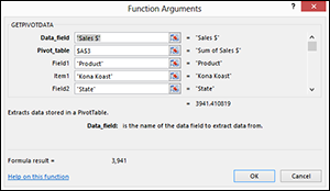
Figure 5-22: The Function Arguments dialog box for the GETPIVOTDATA function.
Arguments of the GETPIVOTDATA function
Here I quickly go through and describe each of the GETPIVOTDATA function arguments. The bulleted list that follows names and describes each argument:
- data_field: The data_field argument names the data field that you want to grab information from. The data_field name in Figure 5-22 is Sales $. This simply names the item that you drop into the Values area of the pivot table.
- pivot_table: The pivot_table argument identifies the pivot table. All you need to do here is to provide a cell reference that’s part of the pivot table. In the GETPIVOTDATA function that I use in Figure 5-21, for example, the pivot_table argument is $A$3. Because cell A3 is at the top-left corner of the pivot table, this is all the identification that the function needs in order to identify the correct pivot table.
- field1 and item1: The field1 and item1 arguments work together to identify which product information that you want the GETPIVOTDATA function to retrieve. Cell C8 holds Kona Koast sales information. Therefore, the field1 argument is product, and the item1 argument is Kona Koast. Together, these two arguments tell Excel to retrieve the Kona Koast product sales information from the pivot table.
- field2 and item2: The field2 and item2 arguments tell Excel to retrieve just Oregon state sales of the Kona Koast product from the pivot table. field2 shows the argument state. item2, which isn't visible in Figure 5-22, shows as Oregon.