
Chapter 10
A Steady State Cash Flow Model
10.1 VALUE AS A FUNCTION OF DISCOUNTED FUTURE RESULTS
In this chapter, we will discuss the three models based on the principle that corporate (and equity value) is a function of the discounted expected future results of a company:
- The first one is based on the formula of capitalization of normalized results. The crucial aspect of this model in the context of company valuation is the assumption that value is linearly dependent on long-term results.
- The second is a growth model in real terms. The crucial elements for the valuation are the factors on which growth is based—that is, the amount of investment necessary to sustain the company's growth and future profitability.
- Third, the multi-stage valuation model, which is based on the concept of limited periods of growth.
The discussion across this and the next chapter will follow this outline:
- Use of a methodology, the Adjusted Present Value (APV), that separately value the unlevered assets of a company and its tax shields distinct
- Proof of the equivalence of the first approach (APV) with the discounted FCFO model and the discounted FCFE model respectively
The equivalence of the results obtained through the different procedures will help us better understand the assumptions implied by the different models.
10.2 CAPITALIZATION OF A NORMALIZED MONETARY FLOW
Under the steady-state scenario, it is assumed that the company can sustain its average cash flow in the long-term through average yearly investments equal to the yearly depreciation. The absence of growth for the company implies that the working capital remains constant. The FCFO therefore coincides with the operating income net of taxes ![]() while the FCFE is equal to the company's net income (NI).
while the FCFE is equal to the company's net income (NI).
Based on previous discussions, the valuation process is quite easy. The value could be determined by simply applying the capitalization formula to the average results projected by experts.
However, it is necessary to realize that capitalization formulas rely on many assumptions, including the fact that cash flows converge to the industry growth rate in the long run and the fact that the discount rate reflects expected price changes as well.
10.2.1 Steady-State Business under Inflationary Conditions
To analyze the issues linked to the use of capitalization formulas, it is necessary to clarify all the different critical aspects.
As previously seen, the assumption that the company needs to be in equilibrium (i.e., in a steady state) is fundamental for the use of synthetic valuation formulas. In particular, in a neutral inflation scenario, the most important assumptions implied by the model are:
The steady-state scenario without real terms growth implies:
- Constant revenues and costs
- New investment equal to yearly depreciation and absence of working capital changes
- A constant debt ratio
When all the aforementioned assumptions hold, cash flows are perpetual and net income is equal to the cash flow available for the shareholders (FCFE).
The neutral inflation scenario requires:
- Uniform price increases of products and services.
- Discount rates reflecting expected price changes.
- No increases in working capital needs; this is consistent with the assumption that current assets are balanced by current liabilities.
- No “paper profit”. This implies that tax-deductible depreciation adjusts to match net investments and that inventory is valued with the LIFO method.
By combining the steady-state assumption with that of neutral inflation, we can define the following equilibrium state for a company:
- Revenues and costs increase linearly every year.
- Net operating cash flow (FCFO) increases proportionally to the inflation rate every year.
- Net financial debt increases every year proportionally to the inflation rate. As a matter of fact, if it did not, the debt ratio would decrease assuming that operating capital increases in nominal terms proportionally to the inflation rate. This would conflict with the steady-state assumption and it would require a different modeling of
 and WACC*.
 - Due to the previous assumption, the FCFE is higher than net income by an amount equal to
 , which is equal to the increase in debt necessary to maintain the target leverage.
10.2.2 An Illustration of the Steady-State/Neutral Inflation Assumption
Exhibit 10.1 shows the cash flow dynamics of a company when the steady-state assumption is combined with a neutral inflation scenario. In particular, we assume that at time zero ![]() prevailing expectation is a 10 percent annual inflation rate. Notice that this inflation rate is particularly high to emphasize its effects.
prevailing expectation is a 10 percent annual inflation rate. Notice that this inflation rate is particularly high to emphasize its effects.
Exhibit 10.1 Steady-state/neutral inflation scenario
| Inflation rate | ||||
| t−1 | t0 | t1 | t2 | |
| Operating margin | 3,000 | 3,300 | 3,630 | 3,993 |
| Depreciation | (500) | (550) | (605) | (665.5) |
| Operating result | 2,500 | 2,750 | 3,025 | 3,327.5 |
| Interests | (200) | (620) | (682) | (750.2) |
| Taxes | (828) | (766.8) | (843.5) | (927.8) |
| Net income | 1,472 | 1,363.2 | 1,499.5 | 1,649.5 |
| Leverage at the end of period | 4,000 | 4,400 | 4,840 | 5,324 |
| FCFO | 1,600 | 1,760 | 1,936 | 2,129.6 |
| FCFE | 1,472 | 1,763 | 1,939.5 | 2,133.5 |
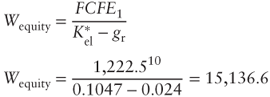
| Wequity | 17,440 | 22,064 | 24,270 | 26,697 |
| D/E | 22.9% | 19.9% | 19.9% | 19.9% |
Column 2 in the table reports the basic data in a company's income statement in a no-inflation scenario ![]() . On the other hand, the other three columns show the results and cash flows for a neutral inflation scenario. The comparison between column 2 and the other three shows the effects of an inflation jump (from 0 to 10 percent).
. On the other hand, the other three columns show the results and cash flows for a neutral inflation scenario. The comparison between column 2 and the other three shows the effects of an inflation jump (from 0 to 10 percent).
The analysis of the last three columns allows us to understand the results and cash flow dynamics in a scenario with inflation (in other words, the analysis of the last three columns allows us to understand the dynamics of the results when inflation is stable at the 10 percent level).
The Effects of an Inflation Jump
By comparing columns 2 and 3 in Exhibit 10.1 we can observe the following:
- The operating income and the FCFO increase by the same percentage as the inflation rate.1
- Interest increases more than the inflation rate as interest rates include expected price changes based on the Fisher principle (see section 4.2). In our example, in the case of zero inflation, the interest rate is assumed to be equal to 5 percent. When the inflation rate is 10 percent, the interest rate becomes:

- The FCFE increases more than the inflation rate because net financial debt is supposed to grow proportionally to the inflation rate so that the debt ratio remains unchanged. In particular, the FCFE at
 is equal to the sum of the net income (which also measures cash flows based on previous assumptions) and the increase in debt in the same period (400).
 - The tax impact on the FCFE decreases since nominal interest, which includes the portion necessary to maintain the real value of the borrowed capital unchanged, is fully deductible.2
At this point, we can conclude that, in a steady-state/neutral inflation scenario, the company value will have to increase proportionally to higher tax savings due to increased interest.
Even though the previous statement is theoretically correct, only a few companies take advantage of an inflation scenario in practice. Many others are in fact penalized. This is due to the fact that revenues and costs are not always linearly related and the company's working capital therefore needs adjustments. This case has not been considered in our analysis since we assume that current assets and current liabilities are balanced.
Cash Flow Dynamic in an Inflation Scenario
The last three columns of Exhibit 10.1 show that the FCFO and the FCFE increase in nominal terms linearly to the inflation rate under a constant inflation rate. It is important to highlight that even interests increase linearly to the inflation rate. As a matter of fact, after the inflation jump, net debt increases annually in a linear fashion with respect to ![]() . This adjustment is necessary to maintain the debt ratio constant.
. This adjustment is necessary to maintain the debt ratio constant.
Let us now verify how the company value can be determined. Let us assume the following parameters:
- Real
 : 8%
: 8% - Nominal
 : 18.8%
 - Real
 : 5%
: 5% - Nominal
 : 15.5%
  : 36%
: 36%
Notice that the valuation takes place at the end of ![]() .
.
Let us begin with the business valuation procedure carried out using the adjusted discount rate approach. Remember that:
| Levered enterprise value | = | Unlevered enterprise value | + | Tax shield |
| = | + |
Estimating the Unlevered Value
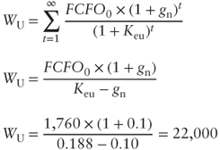
The unlevered value of the company can be determined as the discount of a perpetuity that grows at the inflation rate ![]() :
:
Using the Real Rate
The aforementioned formulas can be presented in another form. In particular, we could split Keu into two elements: the real rate and the expected price change, that is:
We can rewrite [10.1] as:
from which:
which can be simplified as:
The new expression shows a well-known concept. As a matter of fact, in a neutral inflation scenario, the value of an asset generating cash flows and changing proportionally to the inflation rate can be determined by discounting the real cash flow by a real discount rate.
In the example shown in Exhibit 10.1, we obtain:
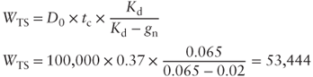
Tax Shield Valuation
Assuming the steady-state/neutral inflation scenario, we know that the value of debt will have to be adjusted for inflation every year. The tax shield value will therefore be equal to:
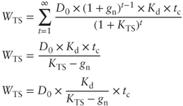
It is important to highlight that ![]() measures the level of debt at the beginning of the period used in estimations. The reason for this choice comes from the assumption that the first interest costs, and therefore the first tax shield, is determined based on the current debt level at the beginning of the period. Interest should, however, be calculated based on the average level of debt for the period under consideration. This is dealt with using acceptable simplification.
measures the level of debt at the beginning of the period used in estimations. The reason for this choice comes from the assumption that the first interest costs, and therefore the first tax shield, is determined based on the current debt level at the beginning of the period. Interest should, however, be calculated based on the average level of debt for the period under consideration. This is dealt with using acceptable simplification.
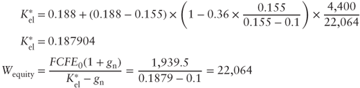
In our example, assuming ![]() , we find:
, we find:
Determining the Levered Value
We can now determine the enterprise levered value as:
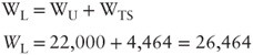
Note that both the unlevered value and ![]() increase in value every year due to inflation. As a matter of fact, also the amount of nominal debt increases linearly to
increase in value every year due to inflation. As a matter of fact, also the amount of nominal debt increases linearly to ![]() .
.
This confirms our conclusion that the unlevered and levered company values increase systematically proportionally to the inflation rate in a steady-state/neutral inflation scenario. Even more importantly, this means that both levered and unlevered companies keep their real value unchanged.
Once ![]() is known, we can then determine the equity value:
is known, we can then determine the equity value:
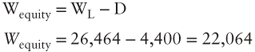
The amount of debt at the end of ![]() is subtracted from
is subtracted from ![]() to determine the value of equity.
to determine the value of equity. ![]() is then the level of debt at the time of the valuation.
is then the level of debt at the time of the valuation.
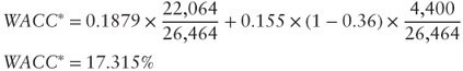
10.2.3 Discount Rate Adjustment Approach
We can now determine the value of the company using adjusted discount rate formulas. To do so, it is necessary to use the formulas presented in the previous chapters for a growth scenario. In particular, the proper formulation is the one consistent with the discount of tax benefits at the rate ![]() .
.
Equity-Side Approach
Let us begin with the equity-side approach:
![]() can be determined through the following formula introduced in previous chapters
can be determined through the following formula introduced in previous chapters
In our case, we find that:
Interestingly, ![]() is paradoxically lower than
is paradoxically lower than ![]() , even if by a small amount. This seems illogical since the risk taken by shareholders is higher when the company is levered. However, we have to go back to the previous results to understand how this result is in fact correct. As we discussed then, the opportunity cost of capital will increase less when tax benefits are present than when they are not. This emphasizes the incremental flow for shareholders coming from tax shields. In our example, tax benefits are so high that (
, even if by a small amount. This seems illogical since the risk taken by shareholders is higher when the company is levered. However, we have to go back to the previous results to understand how this result is in fact correct. As we discussed then, the opportunity cost of capital will increase less when tax benefits are present than when they are not. This emphasizes the incremental flow for shareholders coming from tax shields. In our example, tax benefits are so high that (![]() ) becomes negative. The tax shield value to shareholders is then greater than the loss of value caused by the worsened risk profile caused by higher leverage.
) becomes negative. The tax shield value to shareholders is then greater than the loss of value caused by the worsened risk profile caused by higher leverage.
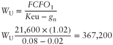
Asset Side Approach
We can now consider the asset side approach:
Based on our example, we can determine that:
And the value is:
Some Concluding Remarks
Our previous discussion introduced all the assumptions and valuation formulas in a steady-state/neutral inflation scenario. It also highlighted the links between the asset-side and equity-side methods.
Nevertheless, the criteria used for the calculation of the company value are particularly aggressive4 for the following reasons:
- As previously mentioned, the neutral inflation hypothesis cannot be accepted for all companies. There are many reasons why this assumption might not hold:
- In some industries, revenues do not readily adjust to costs and replacement costs increase by more than the inflation rate.
- The tax system does not allow for the revaluation of depreciation (except in those countries where inflation is very high and where the technique of inflation accounting is admitted).
- The assumption that inflation does not cause an increase in working capital is not realistic.
- The previously developed method implies that the business maintains a constant leverage in real terms. Being inconsistent with this assumption may cause severe bias in the valuation output.
- If tax benefits from debt are estimated including personal taxes, it is possible that the benefits coming from the deductibility of nominal interest would disappear. As a matter of fact, if nominal interest on business debt is taxed this way, the underwriters of the debt will experience a zero-sum game between their taxes and the benefit obtained by the business.
All this considered, when inflation was a big problem, financial economists concluded that the tax benefit from nominal interest could have offset the disadvantage of not being able to adjust depreciation. On the other hand, the tax benefit could have very rarely created shareholder value (with respect to the scenario with no inflation) contrary to what our previous discussions showed.
10.2.4 Summary of Valuation Formulas Consistent with a Steady-State/Neutral Inflation Scenario
Exhibit 10.2 presents a summary of valuation formulas consistent with the steady-state/neutral inflation hypothesis:
Exhibit 10.2 Valuation formulas in steady-state/neutral inflation scenario
| ASSETS SIDE | APV APPROACH | |
| STANDARD APPROACH | ||
| EQUITY SIDE | STANDARD APPROACH |
To simplify, let us quickly review the meaning of the above symbols:
 : value of the operating capital (asset value)
- FCFO: operating cash flow
- WACC*: weighted average cost of capital when tax shields are present as determined by using [d.1]
 : equity value
- FCFE: cash flow available to shareholders
 : cost of equity, when tax shields are present as determined by using [d]
 : cost of equity of an unlevered company
 : expected inflation rate
At this point, it is important to highlight some important considerations for the application of the above formulas:
- The APV approach has two advantages: transparency and flexibility. Those who perform the valuation appreciate the value component given by
 and the assumptions behind this scenario—that is, the linear relationship between debt and the inflation rate and the presence of tax shields based on the tax rate
  .
. - However, these assumptions are not always credible. For instance, if the company generates cash, it is more realistic to think that the debt amount will decrease. Under these conditions, the APV approach would work better as it allows us to adjust the tax shield value (
 ) to a debt profile consistent with the business plan, the long-term cash flow, and the leverage policy that the management intends to adopt. These specific aspects will be discussed in detail in the following paragraph when analyzing the “Hydroelectric Co.” example.
 - On the other hand, adjusted discount rate formulas face another well-known problem. As a matter of fact, as we previously discussed, the debt ratio used to determine
 and the WACC* should be computed on the basis of the economic value of the business, which, in this case, should include the tax benefits linked to the increase in debt.
Therefore, we can conclude that the process of adjusting discount rates is often used in an approximate way and without a thorough analysis of the underlying assumptions. These assumptions, however, are the key to a correct application of the formulas.
10.2.5 Valuing Hydroelectric Co
The business in this example operates in the electric generation industry.
Assumptions for the valuation:
- The company manages a hydroelectric plant. No expansion of the plant is possible.
- Depreciation is equal, on average, to the investment necessary for the maintenance of the current capacity.
- Management thinks that the current leverage can be maintained in the long term.
- It is assumed that tariffs adjust to costs.
- Current assets and current liabilities tend to balance.
Exhibit 10.3 shows the balance sheet, income statement, FCFO, and FCFE of Hydroelectric Co. at the time of the estimate.
Exhibit 10.3 Hydroelectric Co. financial statements
| BALANCE SHEET | |||
| ACCOUNTS RECEIVABLE | 28,000 | ACCOUNTS PAYABLE | 30,000 |
| INVENTORY | 2,000 | FINANCIAL DEBT | 100,000 |
| NET FIXED ASSETS | 300,000 | SHAREHOLDER EQUITY(*) | 200,000 |
| 330,000 | 330,000 | ||
| (*)Net of income. | |||
| Income Statement | |||
| REVENUES | 90,000 | ||
| OPERATING COSTS | −37,000 | ||
| OPERATING MARGIN | 53,000 | ||
| DEPRECIATION | −14,000 | ||
| EBIT | 39,000 | ||
| FINANCIAL INTERESTS | −7,000 | ||
| TAXES | −14,800 | ||
| NET INCOME | 17,200 | ||
| FCFO | FCFE | ||
| OPERATING MARGIN | 53,000 | 53,000 | |
| INVESTMENTS | −14,000 | −14,000 | |
| CHANGE IN WORKING CAPITAL | – | – | |
| TAXES | −17,400 | −14,800 | |
| FINANCIAL INTERESTS | – | −7,000 | |
| ADJUSTMENTS OF NOMINAL FINANCIAL DEBT (*) | – | 1,961 | |
| 21,600 | 19,161 | ||
* Determined as 2% of the financial debt outstanding at the beginning of the period ![]() .
.
The other important assumptions for the valuation are:
|
8% |
|
|
6.5% |
|
2% |
|
|
37% |
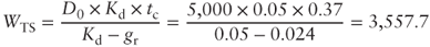
Hydroelectric Co. Valuation: Steady-State/Neutral Inflation Scenario
In order to verify the different results obtained following numerous assumptions, we will use the APV approach to value Hydroelectric Co. It implies, as we know, that:
In this specific case, ![]() can be determined as follows:
can be determined as follows:
![]() can be calculated with the following expressions:
can be calculated with the following expressions:
From which:
With the available data, we can finally determine the equity value by subtracting the value of net financial debt from ![]() (Exhibit 10.3):
(Exhibit 10.3):
Alternative Debt Profiles
It is now possible to check the sensitivity of the value just computed to various debt profiles.
For instance, by observing that the business model of Hydroelectric Co. constantly generates cash flow, it is logical to believe that the debt level will tend to decrease or to at least stay constant.
Under the assumption of decreasing debt and assuming a 10-year debt repayment plan, the value of tax shields will change as shown in Exhibit 10.4.
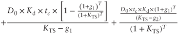
Exhibit 10.4 Debt profile
| |
|
| |
|
| |
|
| |
|
| |
|
| |
|
| |
|
| |
|
| |
The discounted value of the tax shield series using a discount rate Kd= 6.5% is 10.4 million. This amount is 80 percent lower than the result given in an increasing debt scenario (53.4 million).
If we consider the assumption that debt stays constant, the tax shields would become:
Hydroelectric Co. Valuation: The Adjusted Discount Rate Process
It can be interesting to verify our results of the valuation of Hydroelectric Co. with the quick-and-dirty adjusted discount rate process, which is similar to the approaches frequently used in practice.
We calculate the WACC* on the basis of the book value debt ratio:
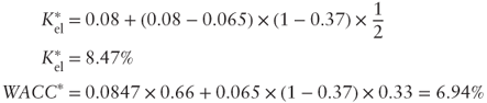
Applying the synthetic approach, we find:
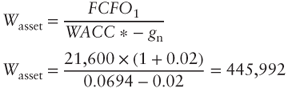
It is interesting to notice that, in a perpetual nominal growth scenario, the value computed under this approach is 25 million greater than the value found through the APV method. Such a result is explained by the use of the book value of debt in the formula, which is higher than the effective one. In fact, economic—and not book—values are supposed to be considered in these formulas. In this specific case, the economic value of equity is significantly higher than the book one, leading to this impressive difference in results.5
10.3 THE PERPETUAL GROWTH FORMULA
We analyzed the impact of nominal growth on value in the previous paragraph.
We now consider the scenario of perpetual growth in real terms. To simplify the analysis, we will refer to a no-inflation scenario.
Growth models are presented in every finance book and wherever valuation and securities analysis are discussed because they allow for the simplification of many problems. They are also the basis to analyze more complex models that will be presented later. Growth formulas are also used in other chapters, where we discuss opportunity cost of capital estimates based on current stock prices and theory of multiples.
The perpetual growth model can be useful to value a business when the business model and the industrial context are such to believe that the cash flow will grow in the long term (at least 20 to 30 years). Therefore, it is better to apply this method to industries that grow in line with the whole economy (e.g. utility companies). Alternatively, it is better to use models based on limited growth assumptions.
10.3.1 Perpetual Growth Model for Unlevered Companies
The perpetual growth model applied to unlevered businesses, that is, to companies with no debt, is known as the Gordon model, named after Myron Gordon, the person who spread its use in the United States of America during the 1950s and 1960s.6
The formula to compute the value of an unlevered company can be presented as follows (notice that when there is no debt, the FCFO and the FCFE coincide):
Let us use an example to better discuss its meaning. Assume that the income statement of a company is:
|
2,500 |
|
0 |
|
(925) |
|
1,575 |
The cash flow dynamic is shown in Exhibit 10.5. The dashed line parallel to the horizontal axis shows the net cash flow of the business available to shareholders (FCFE) in a steady-state scenario. The flow is equal to 1,575 from ![]() to infinity since there are no new investments except renewals, which are equivalent to depreciation in a steady-state scenario.
to infinity since there are no new investments except renewals, which are equivalent to depreciation in a steady-state scenario.
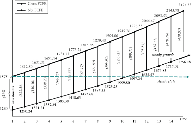
Exhibit 10.5 Cash flow dynamic in a constant-growth scenario
What happens when the company invests 20 percent of its cash flow in new investments for each period? The rate of return for these new investments net of taxes is expected to be 12 percent.
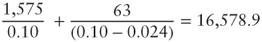
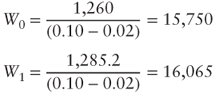
The FCFE at time ![]() is equal to 1,260 (20 percent less than the flow in the steady-state scenario). Furthermore, notice that from
is equal to 1,260 (20 percent less than the flow in the steady-state scenario). Furthermore, notice that from ![]() onward, the cash flow is no longer equal to 1,575, but to 1,612.8 since the reinvestment of 315 in
onward, the cash flow is no longer equal to 1,575, but to 1,612.8 since the reinvestment of 315 in ![]() increases the future flow by 37.8 from
increases the future flow by 37.8 from ![]() to infinity. It is important to mention that the 12 percent rate of return is determined by dividing the reinvested equity amount by the incremental amount net of depreciation. We also assume that depreciation contributes to the systematic renewal of the reinvestment in
to infinity. It is important to mention that the 12 percent rate of return is determined by dividing the reinvested equity amount by the incremental amount net of depreciation. We also assume that depreciation contributes to the systematic renewal of the reinvestment in ![]() .7
.7
In ![]() , the business reinvests 20 percent of its cash flow in the same period (1,612.8). Consequently, the gross cash flow is equal to 1,651.5 (i.e., the sum of the flow in
, the business reinvests 20 percent of its cash flow in the same period (1,612.8). Consequently, the gross cash flow is equal to 1,651.5 (i.e., the sum of the flow in ![]() and the incremental flow of the new investment) from
and the incremental flow of the new investment) from ![]() to infinity. The growth process is limited to a few periods in the table. Nevertheless, we can imagine a scenario in which this recurs for an unlimited period of time.
to infinity. The growth process is limited to a few periods in the table. Nevertheless, we can imagine a scenario in which this recurs for an unlimited period of time.
Characteristics of the Gordon Model
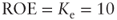
We can now finally introduce some of the major characteristics of this model and its implications:
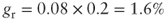
- 1. The net cash flow distributable as shareholder dividends grows at a constant rate (
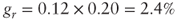
 ) equal to 2.4 percent:
1,260 1,290.24 1,321.2 1,352.9 ……… ∞ 


……… ∞ - 2. The flow before new investments and reinvestments grows at the same rate
 .
. - 3. The rate gr is equal to the rate of return expected from new investments multiplied by the cash reinvestment ratio:
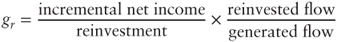
In our example:
- 1. The company value grows yearly based on the same rate gr. As a matter of fact, based on equation [10.5]:
Assuming Keu is equal to 10 percent, then:
- In
 :
: 
- In
 :
: 
It is easy to see that
 is equal to
 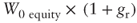 . As a matter of fact:
- In
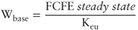
- 1. The value of the business, in a growth scenario, is equal to the sum of the base value calculated in a no-growth scenario (i.e., in the steady-state scenario) and the net present value of the growth opportunities (NPVGO):

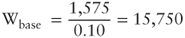
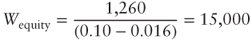
In our example, the base value can be computed by discounting the steady-state scenario FCFE:
On the other hand, NPVGO is equal to the net present value of reinvestments. To be precise, in
 , we will have:
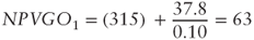
In
 :
: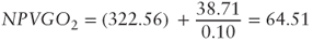
This calculation could be replicated in
 and so on, as long as the firm continues to grow. The cumulate NPVGO of all those reinvestments can be expressed as:
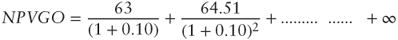
The above calculation, in a perpetual growth scenario, has an infinite number of factors. However, it can be simplified if we consider that the reinvested sums grow at a constant rate gr and the return on new investments stays constant. Hence, the net present value (NPV) will also grow at a constant rate
 . The previous expression then becomes:
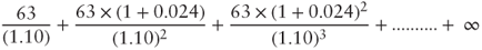
It represents a growing perpetuity at a constant rate, the value of which can be computed using the following formula:8
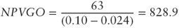
At this point we can verify how the value of a business is formed. Remember that:
- Value of a company in a growth scenario = Wbase + NPVGO
Hence:
- Value of a company in a growth scenario =
The value we just computed is equal to the one we found using the Gordon model in period
 . As a matter of fact:
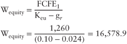
The business valuation model in a growth scenario can be used to verify some well-known principles from which valuation rules derive. In our previous example, we assumed that the return on new investment (12 percent) was greater than the cost of capital (10 percent). Intuitively, we can then state that the growth process creates value in this case. Let us now check what happens if
 percent by modifying Exhibit 10.5.
In Exhibit 10.6, gr is equal to 2 percent. As a matter of fact:
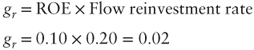
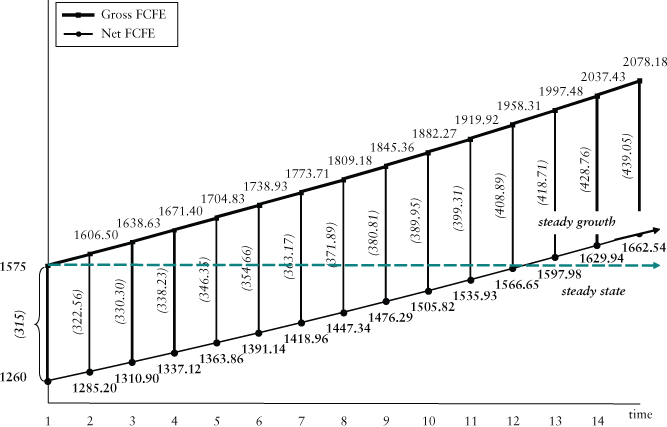
Exhibit 10.6 Flow dynamic in constant growth scenario (ROE = Ke)
Let us now determine the value of the company by using both the steady-state approach and the Gordon model:
- Steady-state approach:
- Gordon model:
We can now state the following:
- 1. The base value of the business under consideration is exactly equal to the one computed using the Gordon model. This conclusion can be surprising once we observe that the business's cash flow and dividends increase every year. At the same time, we can observe that the net present value of growth opportunities is systematically null. As a matter of fact:
The company then increases in size (due to the increase in investments and cash flow), but not in value.
- 2. When the return on new investment equals the cost of capital, the value of the company can be computed by applying the perpetuity formula, that is, by simply discounting the steady-state cash flow. This does not mean that the size of the company or its corresponding cash flows will not grow, but it simply implies that there is no corresponding value creation.
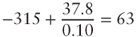
- 3. The value of the company grows in time simply as a reflection of the reinvested sums:
From
 to
to  , the value of the company has grown by 315, which is equal to the amount of money not distributed to shareholders and reinvested into the company.
 - 1. If
 , the growth process destroys value because the NPVGO is negative. We can see this discussing our previous example and assuming that the new investment rate of return is equal to 8 percent. In this case, assuming that the reinvestment is equal to 20 percent of the flow,
  equals:
Consequently, the value computed with the Gordon model is:
By comparing these results with the base value with no investments, we can easily see that the company has destroyed shareholder value by an amount equal to 750.
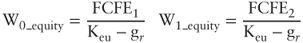
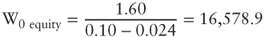
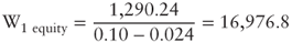
10.3.2 Constant Growth Model for Levered Companies (APV Approach)
We have shown that the value of the company increases proportionally to the ![]() rate when cash flows grow, conditionally to the new investment rate being equal to or greater than the opportunity cost of capital. Assuming that the level of leverage remains constant, the growth process implies that net financial debt will grow year-by-year based on
rate when cash flows grow, conditionally to the new investment rate being equal to or greater than the opportunity cost of capital. Assuming that the level of leverage remains constant, the growth process implies that net financial debt will grow year-by-year based on ![]() . In fact, if this were not the case, the market value of leverage would tend to decrease.
. In fact, if this were not the case, the market value of leverage would tend to decrease.
Let us now analyze the problems linked with the application of growth formulas to levered companies. We will start with the APV approach.
Refer back to our previous example and assume that:
- The operating cash flow (FCFO) reinvestment rate is equal to 20 percent.
- The new investment rate of return on the operating capital is 12 percent.
Also assume the following:
- Net financial debt: 5000
- Interest rate (
 ): 5%
): 5%
Based on these new assumptions, the company's income statement now reports the following results:
| Operating result | 2,500 |
| Interests | (250) |
| Net income before taxes | 2,250 |
| Taxes (37%) | (832.5) |
| Net income (FCFE) | 1,417.5 |
As we know, the levered value of the company is equal to the sum of its unlevered value and the value of the net tax shield:
- Unlevered value of the company in a growth scenario:
This value is equal to the one derived in the preceding paragraph.
- Tax shield (when
 ):
):
It is important to highlight that ![]() is equal to 5,000 because it is assumed that the company will make its first investment at the end of
is equal to 5,000 because it is assumed that the company will make its first investment at the end of ![]() and it will take on debt at the same time. Therefore, the first tax shield refers to current debt (=5000)
and it will take on debt at the same time. Therefore, the first tax shield refers to current debt (=5000)
- Levered company value:

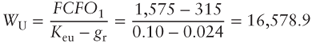
As in the example discussed in the previous paragraph, the computed value can be divided into two parts: the base value and the net present value of growth opportunities. Using the data from the previous example, we have the following:
- Unlevered NPVGO:
- Tax shield value:
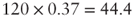
The unlevered NPVGO is equal to the difference between the total investment in ![]() and the net present value of the incremental flow (FCFO). The tax shield from the investment in
and the net present value of the incremental flow (FCFO). The tax shield from the investment in ![]() is equal to the debt undertaken to finance the investment multiplied by the tax rate. This tax rate expresses the savings linked to the tax shield (in the case of a perpetuity:
is equal to the debt undertaken to finance the investment multiplied by the tax rate. This tax rate expresses the savings linked to the tax shield (in the case of a perpetuity: ![]() ).
).
The expected value of all growth opportunities is:
- Unlevered NPVGO =
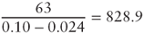
- Tax shield =
To summarize, we9 can break up and reaggregate the components of the value of the company as determined by the APV approach:
| Unlevered base value9 | 15,750.0 |
| Unlevered NPVGO | 828.9 |
| Unlevered value in growth scenario | 16,578.9 |
| Base value of tax shields | 1,850.0 |
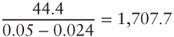
| Value of incremental tax shields | 1,707.7 |
| Unlevered company value in growth scenario | 20,136.6 |
Our previous discussion highlights a very important conclusion: the creation of value in a growth scenario is mostly due to the incremental tax shield linked to the increase (based on ![]() ) in debt. This is another crucial point to bear in mind when using the constant growth models. As a matter of fact:
) in debt. This is another crucial point to bear in mind when using the constant growth models. As a matter of fact:
- The rate leading to the exact value of the tax shield can be less than
 .
. - It is not certain that the company can systematically use tax shields related to its interest payments.
- The hypothesis of using
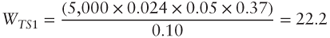
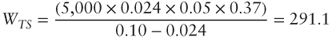
 in order to discount the incremental tax shields is not at all prudent. In our previous example, if
  were to be determined using
  , the tax shield value would consistently decrease from 1707.7 to 291.1. As a matter of fact:
 - The tax shield value from the first reinvestment is:
- The net present value of all tax shields instead equals:
10.3.3 Discount Rate Adjustment Methods
In the perpetual growth scenario, the use of the adjusted discount rate formulas requires the same caution as the nominal growth approach discussed in the previous subsection. Specifically:
- We should use the same formulas consistent with the tax shield discount rate chosen by the expert to determine
 and the WACC*.
 - The debt ratio should be expressed based on the economic equity value, which should include the net present value of the incremental tax shields.
Going back to the value of equity computed through the APV method, it is possible to verify the use of the adjusted discount rate formulas when discounting the tax shields at ![]() :
:
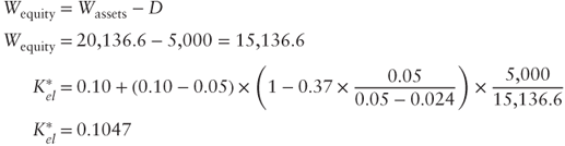
Once ![]() is computed, we can determine
is computed, we can determine ![]() with the usual adjusted discount rate process:
with the usual adjusted discount rate process:
The10 value determined above corresponds to the one computed through the APV process. The same result can be obtained starting from the asset-side perspective by using the WACC* and the ![]() .
.
10.3.4 Steady-Growth Scenario: A Wrap-up
Exhibit 10.7 shows a summary of the valuation formulas consistent with a constant growth scenario.
Exhibit 10.7 Valuation formulas in a perpetual growth scenario
| ASSETS SIDE | APV APPROACH | |
| STANDARD APPROACH | ||
| EQUITY SIDE | STANDARD APPROACH |
They are similar to those previously examined at the beginning of this chapter. However, the application of these formulae is more complex. To be precise, there could be issues linked to real growth scenarios as well as to the use of ![]() in the computation of the net present value of tax shields.
in the computation of the net present value of tax shields.
It is also necessary to check the methods used in the computation of the FCFO and the FCFE. In the case of real growth, they should be computed consistently with the reinvestment needed to sustain growth in real terms.
For convenience, we will recall the meaning of the above symbols:
 = operating capital value (asset value)
 = equity value
 = expected operating cash flow at time 1
 = expected equity cash flow at time 1
 = weighted average cost of capital when tax benefits are present, as determined by using the appropriate formulas and the chosen tax rate
 = equity cost of capital when there are tax benefits, as determined by the appropriate formulas and the chosen rate
 =equity cost of capital for an unlevered company
 = cash flow growth rate in real terms
 = tax rate
 = net financial debt at the beginning of the period
 = cost of debt
 = tax benefit discount rate
The formulas are the same as those in Exhibit 10.2 in which we assume, however, that the tax benefits are discounted using ![]() . This hypothesis can be modified even if we are in a steady-state scenario.
. This hypothesis can be modified even if we are in a steady-state scenario.
10.4 FORMULAS FOR LIMITED AND VARIABLE (MULTI-STAGE) GROWTH
In the previous section we observed that the perpetual constant growth formula implies an “aggressive” valuation approach. The main issue linked to this method is that we can rarely prove a relationship between unlimited real-term growth of an industry and macroeconomic variables. This assumption mostly holds for companies such as the utility ones.
Apart from these exceptions, it is preferable to assume that growth is limited. As a matter of fact, once the expansion period is over, a company is then characterized by an equilibrium phase (steady state). In such a case, perpetual growth formulas are substituted by limited growth formulas, which are represented as follows:
| ASSETS SIDE | APV APPROACH | 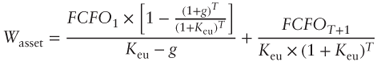 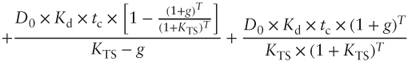 |
| STANDARD APPROACH | 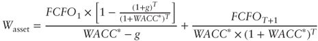 |
|
| EQUITY SIDE | STANDARD APPROACH | 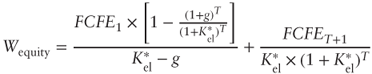 |
It is crucial to highlight that rates are expressed in nominal terms. This means that, once the growth period is over, the FCFO and the tax shields do not increase proportionally to inflation. If such an assumption cannot be proven to hold, the expert should use variable-growth formulas. Assume a value equal to the expected inflation rate for g2. For simplicity, we will once again remind the reader of the meaning of the above symbols:
 = operating capital value (asset value)
 = equity value
 = expected operating cash flow at time 1
 = expected equity cash flow at time 1
 = weighted average cost of capital when tax benefits are present, as determined by using the appropriate formulas and the chosen tax rate
 = equity cost of capital when there are tax benefits, as determined by the appropriate formulas and the chosen rate
 = equity cost of capital for an unlevered company
 = (limited) growth rate for cash flows
 = tax rate
 = net financial debt at the beginning of the period
 = cost of debt
 = discount rate for tax shields
Variable-growth formulas are useful when the valuation assumptions require consideration of different growth rates for different time periods. For instance, they would require a strong growth period for the first few years and then a more moderate growth rate once the exceptional growth is over. Some finance textbooks present what is referred to as a three-stage formula. However, for practical purposes, they tend to be a useless complication.
Exhibit 10.9 demonstrates variable-growth formulas, where:
Exhibit 10.9 Valuation formulas in a variable-growth scenario
| ASSETS SIDE | APV APPROACH | 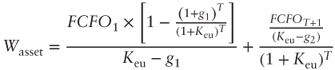
 |
| STANDARD APPROACH | 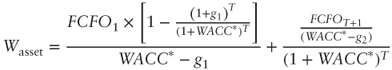 |
|
| EQUITY SIDE | STANDARD APPROACH | 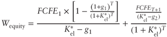 |
| = | operating capital value (asset value) | |
| = | equity value | |
| = | expected operating cash flow at time 1 | |
| = | expected equity cash flow at time 1 | |
| = | weighted average cost of capital when tax shields are present, as determined by using the appropriate formulas and the chosen tax rate | |
| = | equity cost of capital when there are tax shields, as determined by the appropriate formulas and the chosen rate | |
| = | equity cost of capital for an unlevered company | |
| = | cash flow growth rate in the [1,T] period | |
| = | cash flow growth rate from T+1 | |
| = | tax rate | |
| = | net financial debt at the beginning of the period | |
| = | cost of debt | |
| = | discount rate for tax shields |
The above formulas express a two-stage estimate approach. As a matter of fact, it is assumed that the business valuation is based on the hypothesis that cash flows grow at a rate equal to ![]() up to
up to ![]() , and at
, and at ![]() from then on.
from then on.
10.5 CONCLUSIONS
Limited- and variable-growth formulas do not require to be analyzed in more depth. The possible application problems and distortions have already been covered in the previous two paragraphs when discussing the formula for the capitalization of expected cash flows and the perpetual constant growth formula.
Generally, limited- and variable-growth formulas are used to make estimates of company values with relatively small ![]() and
and ![]() . Alternatively, it would make more sense to use an analytical valuation process inclusive of a terminal value. As a matter of fact, in these cases, strong growth periods are characterized by changing cash flows, which should be represented explicitly.
. Alternatively, it would make more sense to use an analytical valuation process inclusive of a terminal value. As a matter of fact, in these cases, strong growth periods are characterized by changing cash flows, which should be represented explicitly.
In practical applications, ![]() is frequently equal to the expected long-run growth rates of macroeconomic variables such as GDP or the consumption rate. Such an assumption is valid only if it can be proven that there exists a strong correlation between the industry growth rate and GDP. This usually happens, as we have previously mentioned, in public utilities and banking/insurance sectors.
is frequently equal to the expected long-run growth rates of macroeconomic variables such as GDP or the consumption rate. Such an assumption is valid only if it can be proven that there exists a strong correlation between the industry growth rate and GDP. This usually happens, as we have previously mentioned, in public utilities and banking/insurance sectors.
If there is no correlation, ![]() is purely a subjective choice.
is purely a subjective choice.
Finally, it is important to mention that ![]() and
and ![]() also incorporate the nominal growth, which is linked to the expected price variation.
also incorporate the nominal growth, which is linked to the expected price variation.
It is worth mentioning that, in case of temporary or variable growth, the value obtained by applying the APV approach does not necessarily match the one derived from the procedure based on the standard DCF approach. As already noted, such equivalence holds only when ![]() .
.
____________________