3
Software development tools and the TMS320C6678 EVM
3.1 Introduction
There has been massive growth in real‐time applications demanding real‐time processing power, and this has led DSP manufacturers to produce advanced chips and advanced development tools which not only allow engineers to develop complex algorithms with ease but also speed up time‐to‐market. Development tools can be divided into hardware and software development tools (see Figure 3.1). Development tools are very important and tend to shorten significantly the development time, which is itself the most time‐consuming part of the production of a device.
Figure 3.1 Hardware and software development tools.
Texas Instruments (TI) provides an advanced integrated software and hardware development toolset. On the software side, it provides the Multicore Software Development Kit (MCSDK) that provides foundational software for the KeyStone devices as shown in Figure 3.2. On the host side, the main part in the MCSDK is the Code Composer StudioTM (CCS) Integrated Development Environment (IDE) which is based on Eclipse, an open‐source software framework used by many embedded software vendors. Included in CCS are a full suite of compilers (which support OpenMP) [1], a source code editor, a project building environment, a debugger, a profiler, an analyser suite, and many other code development capabilities (see video in Ref. [2]). On the target side, it includes mainly the instrument and trace, symmetric multiprocessing (SMP) Linux for ARM and other libraries.
Figure 3.2 Texas Instruments’ software ecosystem [3].
CCS has been developed in such a way that its functionality can be extended by plug‐ins. There are two types of plug‐ins: ones written by TI and ones written by a third party. Some plug‐ins are very useful as they provide graphical development tools which are intuitive and abstract device APIs (application programming interfaces) and hardware details. For instance, with a few clicks of the mouse, one can configure some interrupts, a peripheral or a debugging procedure.
It is essential for a developer to fully understand the use and capabilities of the tools. This chapter is divided into three main parts: the first part describes the development tools, the second part describes the evaluation module (EVM) and finally the third part describes provided laboratory exercises demonstrating the capabilities of the CCS and EVMs.
3.2 Software development tools
The software development tools consist of the following modules: the C‐compiler, assembler, linker, simulator and code converter (see Figure 3.3).
Figure 3.3 Basic development tools.
If the source code is written in C language, the code should be compiled using the optimising C compiler provided by TI [4]. This compiler will translate the C source code into an assembly code. The assembly code generated by either the programmer, the compiler or the linear assembler (see Chapter 5) is then passed through the assembler that translates the code into object code. The resultant object files, any library code and a command file are all combined by the linker which produces a single executable file. The command file mainly provides the target hardware information to the linker and is described in Section 3.2.3.1.
3.2.1 Compiler
The C code is not executable code and therefore needs to be translated to a language that the DSP understands. In general, programs are written in C language because of its portability, ease of use and popularity. Although for time‐critical applications assembly is the most efficient language, the optimising C compiler for the TMS320C66x processors can achieve performances exceeding 70% compared with code written in assembly. This has the advantage of reducing the time‐to‐market and hence cost.
To evoke the compiler, use the CL6x command as shown here:
Note: The CL6x command is not case sensitive for Windows.
The compiler uses options supplied by the user. These options provide information about the program and the system to the compiler. The most common options are described in Chapter 5. However, for a complete description of the compiler options, the reader is referred to the optimising C compiler manual [4].
The options shown in Table 3.1 can be inserted between the CL6x command and the file name as shown here:
Table 3.1 Common compiler options
| Option | Description |
| ‐mv6600 | Tells the compiler that the code is for the TMS320C66x processor |
| ‐k | Do not delete the assembly file (*.asm) created by the compiler. |
| ‐g | Symbolic debugging directives are generated to enable debugging. |
| ‐i | Specifies the directory where the #include files reside |
| ‐s | Interlists C and assembly source statements |
| ‐z | Adding the ‐z option to the command line will evoke the assembler and the linker. |
3.2.2 Assembler
The assembler translates the assembly code into an object code that the processor can execute. To evoke the assembler, type:
The above command line assembles the FIR1.asm file and generates the FIR.obj file. If ‘FIR.obj’ is omitted from the command, the assembler automatically generates an object file with the same name as the input file but with the .obj extension, in this case FIR1.obj.
Note: The asm6x command is not case sensitive for Windows.
The assembler, as with the compiler, also has a number of ‘switches’ that the programmer can supply. The most common options are shown in Table 3.2.
Table 3.2 Common assembler options
| Option | Description |
| ‐l | Generates an assembly listing file |
| ‐s | Puts labels in the symbolic table in order to be used by the debugger |
| ‐x | Generates a symbolic cross‐reference table in the listing file (using the ‐ax option automatically evokes the ‐l option) |
The following command line assembles the FIR1.asm file and generates an object file called fir1.obj and a listing file called fir1_lst.lst.
Note: The file names are case sensitive.
3.2.3 Linker
The various object files which constitute an application are all combined by the linker to produce a single executable file. The linker also takes as inputs the library files and the command file that describes the hardware. To evoke the linker, type:
The above command line links the FIR1.obj file with the file(s) contained in the command file comd.cmd. The linker options can also be contained in the command file.
The linker also has different options that are specified by the programmer. The most common options are shown in Table 3.3.
Table 3.3 Frequently used options for the linker
| Options | Description |
| ‐o | Names an output file |
| ‐c | Uses auto‐initialisation at runtime |
| ‐l | Specifies a library file |
| ‐m | Produces a map file |
The following command line links the file FIR1.obj with the file(s) specified in the comd.cmd file and generates a map file (FIR1.map) and an output file (FIR1.out).
Note: The ‐m FIR1.map and the ‐o FIR1.out command could be included in the command file.
Note: The lnk6x command is not case sensitive for Windows, and if ‐o FIR1.out is omitted, then an A.out file will be generated instead.
3.2.3.1 Linker command file
The command file serves three main objectives: the first objective is to describe to the linker the memory map of the system to be used, and this is specified by ‘MEMORY {…}’. The second objective is to tell the linker how to bind each section of the program to a specific section as defined by the MEMORY area; this is specified by ‘SECTIONS {…}’. The third objective is to supply the linker with the input and output files, and options of the linker. An excerpt of a command file for the TMS320C6678 EVM is shown in Figure 3.4.
Figure 3.4 Excerpt of command file for the TMS320C6678 EVM (C6678.cmd).
As with all embedded systems, the command file is indispensable for real‐time applications. The linker options specified in the CL6x command can be specified within the command file, as shown in Figure 3.4.
3.2.4 Compile, assemble and link
The command CL6x, combined with the ‐z linker option, can accomplish the compiling, assembling and linking stages all with a single command, as shown here:
3.2.5 Using the Real‐Time Software Components (RTSC) tools
By using the RTSC tools, one is able to take advantage of the higher levels of programming and performance that the RTSC can offer in addition to features that allow components to be added or modified/upgraded without the need to modify the source code. For a complete description of the RTSC, please refer to Ref. [5].
The XDCtools are the heart of the RTSC components; see Figure 3.5. These tools provide mainly efficient APIs for development and static configurations that can accelerate development to production time and ease maintenance.
Figure 3.5 RTSC tools [6].
3.2.5.1 Platform update using the XDCtools
In Section 3.2.3, a command file was written from scratch. With the use of the XDCtools, this can be imported as a package that is delivered by the developer (TI) and used by the consumer. This package can be in the form of a plug‐in.
In the example shown in Figure 3.6, instead of entering a linker command file, a platform file describing the memory map is supplied (see Figure 3.7). This platform can be viewed and modified by selecting (while in the CCS Debug mode) Tools → RTSC Tools → Platform → New. Figure 3.7 to Figure 3.12 are self‐explanatory on how to generate a new target platform from a seed platform. Once a platform is created, the seed platform has to be replaced by the new platform, as shown in Figure 3.13.
Figure 3.6 Entering a linker command file.
Figure 3.7 Platform selection.
Figure 3.9 Selecting the device family and device name for the new platform.
Add the path shown in Figure 3.12 (C:UserseendmyRepositorpackages) using the Add button shown in Figure 3.13, then select the platform myBoard.
Figure 3.12 Output when a successful platform is generated.
Figure 3.13 Selecting the new platform for the project.
3.2.6 KeyStone Multicore Software Development Kit
The KeyStone System‐on‐Chip (SoC) is a very powerful and complex processor. To ease its use and reduce time‐to‐market, TI has developed foundation software called the Multicore Software Development Kit (MCSDK); see Figure 3.14 [7]. The MCSDK, with the supported EVMs, provide out‐of‐box demos with source code that can be modified, libraries and device drivers. TI also provides a platform development kit with low‐level software drivers, libraries and chip support software for peripherals supported by the KeyStone [8].
Figure 3.14 Multicore Software Development Kit (MCSDK) [9, 10].
3.3 Hardware development tools
EVMs are relatively low‐cost demonstration boards. They allow one to evaluate the performance of the processors. The EVMs are platforms that contain the processor, some peripherals, expansion connectors and emulators. In the case of the TMDXEVM6678LE EVM, there are two emulators, one on‐board (XDS100) and one on a mezzanine (XDS560), that use the JTAG (Joint Test Action Group) emulator header, as shown in Figure 3.15a. The KeyStone II has a Mezzanine XDS200 emulator connected to the JTAG header, as shown in Figure 3.15b.
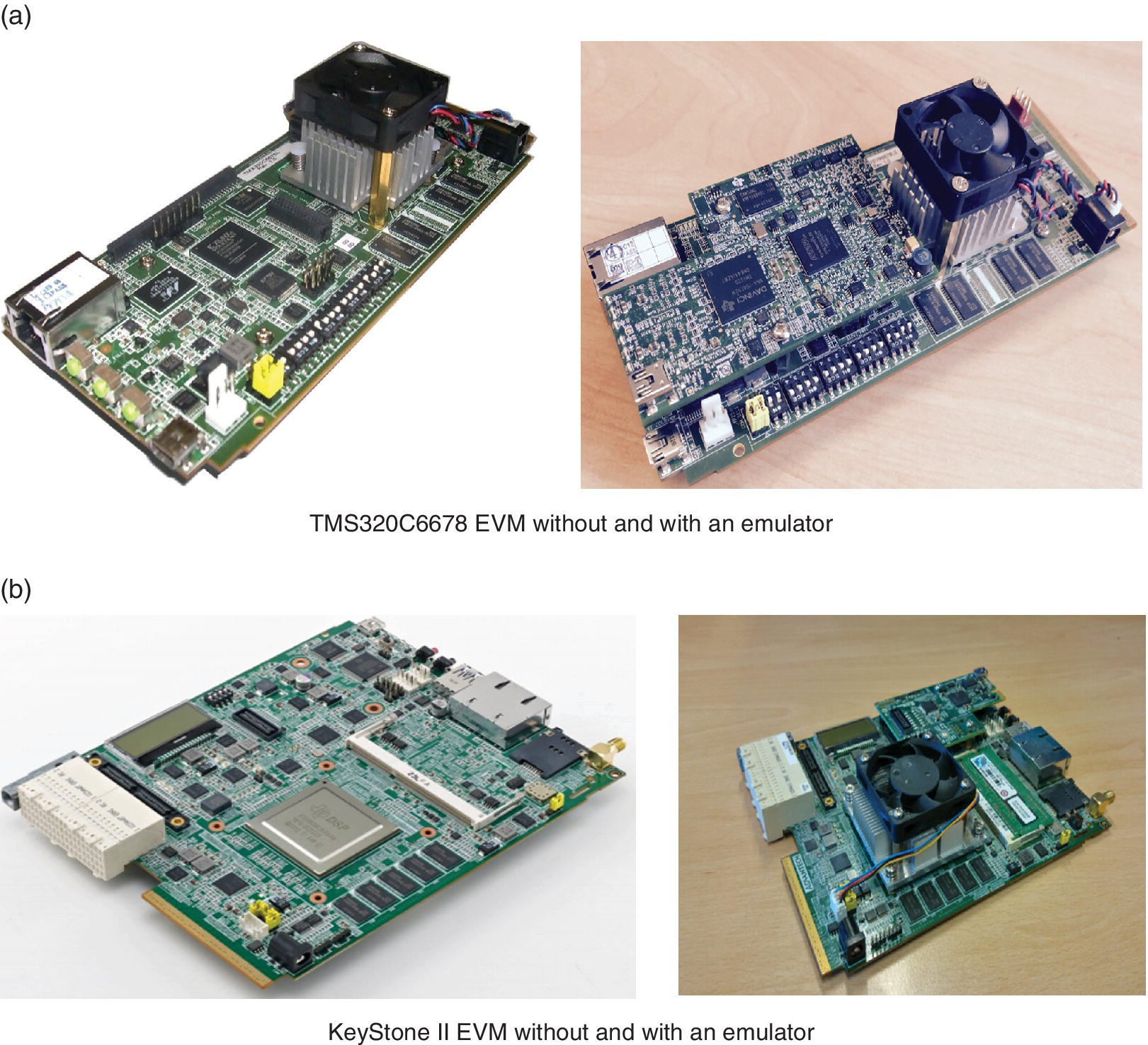
Figure 3.15 The TMS320C6678 and the KeyStone II EVMs. (a) TMS320C6678 EVM without and with an emulator; (b) KeyStone II EVM without and with an emulator.
Note: In this book, two EVMs are used: the TMDXEVM6678LE and the K2EVM‐HK. For a complete description, please refer to Refs. [7] and [11–13].
The basic layouts of both EVMs are shown in Figure 3.16.
Figure 3.16 EVM layout. (a) TMS320C6678L [14]; (b) KeyStone II [15].
3.3.1 EVM features
The key features of the TMDXEVM6678L or TMDXEVM6678LE EVM are [16]:
- TI’s multicore DSP – TMS320C6678
- 512 MB of double data rate type 3 (DDR3)‐1333 memory
- 64 MB of NAND (‘not AND’) flash
- 16 MB of serial peripheral interface (SPI) NOR (‘not OR’) flash
- Two Gigabit Ethernet ports supporting 10/100/1000 Mbps data rates – one Advanced Mezzanine Card (AMC) connector and one RJ‐45 connector
- 170‐pin B + ‐style AMC interface containing serial RapidIO (SRIO), PCI Express (PCIe), Gigabit Ethernet and time‐division multiplexing (TDM)
- High‐performance connector for HyperLink
- 128 KB inter‐integrated circuit (I2C) electrically erasable programmable read‐only memory (EEPROM) for booting
- Two user light‐emitting diodes (LEDs), five banks of dual in‐line package (DIP) switches and four software‐controlled LEDs
- RS232 serial interface on a 3‐pin header or Universal Asynchronous Receiver/Transmitter (UART) over a mini‐USB connector
- External memory interface (EMIF), timer, SPI and UART on 80‐pin expansion header
- On‐board XDS100 type emulation using high‐speed USB 2.0 interface
- TI 60‐pin JTAG header to support all external emulator types
- Module Management Controller (MMC) for the Intelligent Platform Management Interface (IPMI)
- Optional XDS560v2 System Trace Emulator mezzanine card
- Powered by DC power‐brick adaptor (12 V/3.0 A) or AMC Carrier backplane
- PICMG® AMC.0 R2.0 single‐width, full‐height AMC module.
The key features of the KeyStone II EVM are [15]:
- TI’s 8‐core DSP and 4‐core ARM SoC
- 1024/2048 MB of DDR3‐1600 memory on board
- 2048 MB of DDR3‐1333 error‐correcting code (ECC) small‐outline dual‐inline memory module (SO‐DIMM)
- 512 MB of NAND flash
- 16 MB SPI NOR flash
- Four Gigabit Ethernet ports supporting 10/100/1000 Mbps data rate
- AMC connector and two RJ‐45 connectors
- 170‐pin B + ‐style AMC interface containing SRIO, PCIe, Gigabit Ethernet, Architecture Antenna Interface 2 (AIF2) and TDM
- Two 160‐pin ZD + ‐style universal reversible Turing machine (uRTM) interfaces containing HyperLink, AIF2 and XGMII (not supported for all EVMs)
- 128 KB I2C EEPROM for booting
- Four user LEDs, one bank of DIP switches and three software‐controlled LEDs
- Two RS232 serial interfaces on a 4‐pin header or a UART over a mini‐USB connector
- EMIF, timer, I2C, SPI and UART on a 120‐pin expansion header
- One USB 3.0 port supporting a 5 Gbps data rate
- MIPI 60‐pin JTAG header to support all external emulator types
- LCD display for debugging state
- Microcontroller unit (MCU) for the IPMI
- Optional XDS200 System Trace Emulator mezzanine card
- Powered by DC power‐brick adaptor (12 V/7.0 A) or AMC Carrier backplane
- PICMG® AMC.0 R2.0 and uTCA.4 R1.0 double‐width, full‐height AMC module.
3.4 Laboratory experiments based on the C6678 EVM: introduction to Code Composer Studio (CCS)
All laboratories experiments have been tested, and solutions are provided.
File location
- Chapter_3_Code:
3.4.1 Software and hardware requirements
- CCS version 6.0 or higher: CCS6.0 (see Figure 3.17)
- PC with the following hardware and software:
Minimum Recommended Memory 1 GB 4 GB Disk space 300 MB 2 GB Processor 1.5 GHz single core Dual core - Operating system requirements for the PC:
- Windows. Windows XP, 7, 8 or 10.
- Linux. Details on the Linux distributions supported are available in Ref. [17].
- A TMX320C6678 EVM. The EVM used in this laboratory experiment is based on the TMS320C6678 EVM module shown in Figure 3.18.
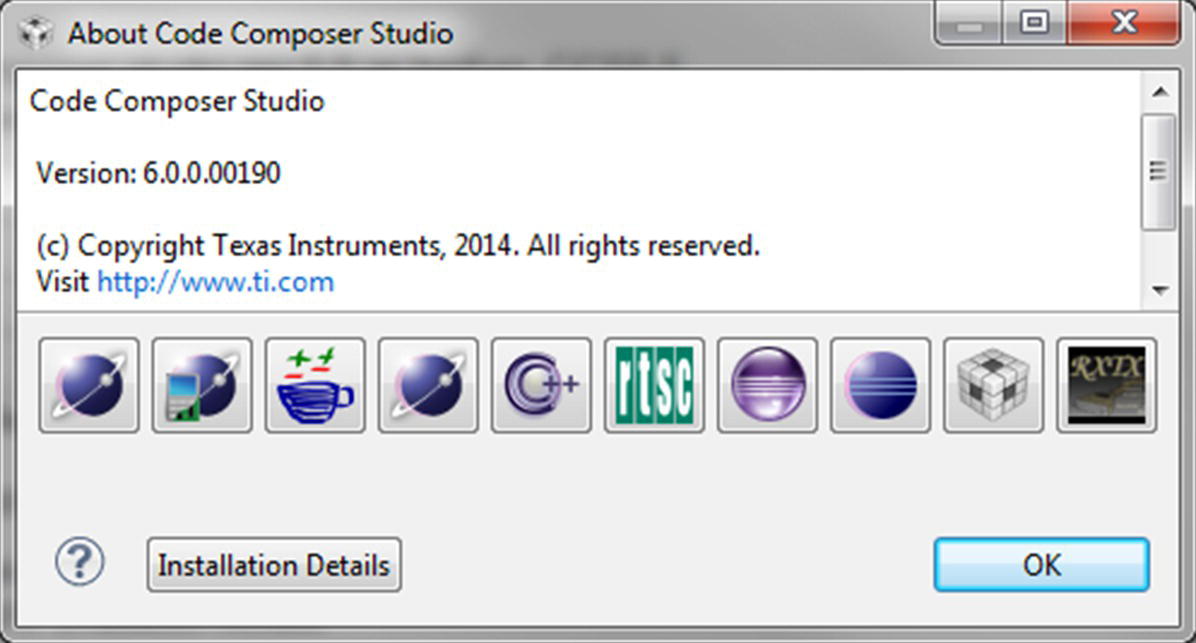
Figure 3.17 Code Composer Studio (CCS).
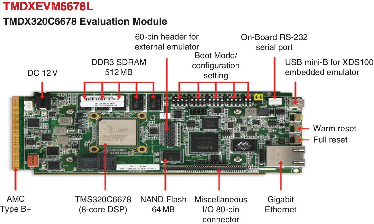
Figure 3.18 The TMS320C6678 EVM.
3.4.1.1 Key features
| Hardware features | Software features | Kit contents |
|
|
|
3.4.1.2 Download sites
Follow these links to access the sites required.
- Wiki: Code Composer Studio. Information on how to more effectively use the CCS.
- Download site. All current and archived product images.
- HELP: having trouble? Where to go for downloads, upgrades, licencing and subscription help. http://www.ti.com/lsds/ti/software‐help.page
- System requirements. Details on the minimum and recommended system requirements.
- Subscription information. Details on the CCS subscription service (no subscription required).
For this teaching material, download the Windows version shown in Figure 3.19. You will be prompted to register with TI.com as shown in Figure 3.20. Once registered, you will be given access to download the CCS as shown in Figure 3.21.
Figure 3.19 CCS download page.
Figure 3.20 Registration with myTI.
Figure 3.21 CCS download.
3.4.2 Laboratory experiments with the CCS6
These laboratory experiments mainly provide an introduction to the CCS, implementation of a dot product (dotp), how to use the CCS clock to benchmark code and how to download code to separate cores and run them on the TMS320C6678 EVM.
File locations for this chapter:
- Chapter_3_Codedotp
- Chapter_3_CodePrint_Functions
3.4.2.1 Introduction to CCS
The aim of this laboratory exercise is to become familiar with the DSP tools and to be introduced to programming the TMS320C66xx SoC DSP.
This section shows how to use development tools, create a project and modify the compiler switches in order to achieve the best performance.
Starting the experiment
- Launch CCS. Launch CCS by double‐clicking on the desktop icon of your PC or using: Start > All Programs > Code Composer Studio 6.0.0 (or a later version). You should see a CCS window, as shown in Figure 3.22, if you run the CCS for the first time; or the screen will look like Figure 3.23 if the CCS has been used before.
Note: You have to be logged in as an administrator if you require updates.
- Create a new project. A project stores all the information needed to build an individual program or library, including:
- File names of source code and object libraries
- Build‐tool options
- File dependencies
- A build‐tool version used to build the project.
- Select File > New > CCS Project (see Figure 3.24).
Note: DO NOT press ‘Finish’ until you have configured your project.
- Set up the project settings according to the screenshot given in Figure 3.24.
- Insert the target.
- Select the device family and variant.
- Select the connection (the XDS560v2‐USB Mezzanine Emulator is used).
- Select the compiler version.
- Choose the Hello Word template.
- Check Advanced Settings (see Figure 3.25). Even though this dialogue is HIDDEN and called Advanced, it is CRITICAL to check this to make sure you are creating a project with the right tools, endianness and output format.
Note: If you import a project and you do not have the right compiler or XDCtools version, you can download them separately using these links:
https://www‐a.ti.com/downloads/sds_support/TICodegenerationTools/download.htm
http://downloads.ti.com/dsps/dsps_public_sw/sdo_sb/targetcontent/rtsc/
However, you may have to register with TI first. Once the tools are downloaded and installed, restart the CCS so that the tools will be automatically updated.
Press ‘Finish’ to confirm the settings. The window in Figure 3.26 will then appear.
- Edit perspective (see Figure 3.27). Once you create a project, you will have two default perspectives, one for editing (CCS Edit) and one for debugging (CCS Debug). Make sure you select the appropriate perspective for what you want to do.
- Adding a DSP target configuration (see Figure 3.28). The target configuration is used by the debugger. You can have one project with many target configurations and therefore many platforms (e.g. a simulator or an EVM). This is very convenient as no modification to your project is required when you change emulators.
Once you have defined a project, you can add a configuration to this project using these commands:
- Select the project in Project Explorer, and then select the File > New > Target Configuration File command from the main menu.
Type a file name, and click Finish.
Select File > Save As (
 ) to record your target configuration selections.
Open the target configuration and set it for the Blackhawk XDS560v2‐USB Mezzanine Emulator and the TMS320C6678, as shown in Figure 3.29.
Select the Advanced tab and explore the CPU Properties. Then, save and close the file.
Note: You can add multiple target configurations to your projects (this is very useful if you are using different platforms). However, only one target configuration can be active at any time. You can also choose a default target so that you don’t have to add a target configuration to each project.
To add a new target configuration to the list of target configurations or to select a new configuration for a project, do the following:
- Select View > Target Configurations.
- Right‐click on User Defined.
- Select the appropriate target.
- Select the appropriate function and close the window (see Figure 3.30).
By selecting one of the commands from the list, a display of the New Target Configuration dialogue will appear as shown in Figure 3.30.
You can now see all the configurations created and their locations. Now you can select the appropriate configuration. In this laboratory, you will be using the configuration that you just created.
Once the target configuration is completed and closed, it will be automatically added to your project and set to Active.
Go back to the Project Explorer. If your Project Explorer is not visible, then select Project Explorer (see Figure 3.31).
- Select the project in Project Explorer, and then select the File > New > Target Configuration File command from the main menu.
- Building and loading the code (see Figure 3.32)
Notice that the project is highlighted and there is [Active – Debug] next to the project name. This means:
- Highlighted: The project is active (only one project can be active at a time).
- Active: The project is active.
- Debug: The project is in the debug mode.
Right‐click on the project and select Build Configurations → Set Active.
Click on Release, and see Debug change to Release in the project. This is how you change build configurations (the set of build options) when you build your code.
Note: Build configurations such as Debug, Release and others that you create will not contain the same build options, like levels of optimisation and debug symbols; specify file search paths for libraries (‐l) and include search paths (‐i) for included directories.
Change the build configuration back to Debug. Near the top left‐hand corner of CCS, you will see the build Hammer and the Bug:
- The Hammer allows you to change the build configuration (Figure 3.33 and Figure 3.34) and build your project.
- The Bug allows you to debug the code.
Select the Debug mode, and start debugging your code.
If you simply click the bug, it will build whichever configuration is set as the default (either Debug or Release). It will always do an incremental build (i.e. build only those files that have changed since the last build; it is much faster this way).
You can also specify a build type as shown in Figure 3.35.
There are three kinds of builds:
- Build
- Clean build
- Rebuild.
Incremental and clean builds can be done over a specific set of projects or the workspace as a whole. Specific files and folders cannot be built. There are two ways that builds can be performed:
- Automatic builds are performed as resources are saved. Automatic builds are always incremental and always operate over the entire workspace. You can configure your preferences (Window > Preferences > General > Workspace) to perform builds automatically on resource modification.
- Manual builds are initiated when you explicitly select a menu item or press the equivalent shortcut key. Manual builds can be either clean or incremental and can operate over collections of projects or the entire workspace.
- Running the project. To run the project, press the bug as shown in Figure 3.33. If the EVM is connected properly and the project successfully built, then the window shown in Figure 3.36 will appear.
Once you have successfully built your project, the Debug window will appear as shown in Figure 3.37.
You can observe the CDT Build Console to see the compilation feedback. If the window is not visible, choose View > Console. In fact, View lets you select a list of windows that you would like to display; see Figure 3.38.
Figure 3.22 CCS starting window.
Figure 3.23 Selecting a workspace location.
Figure 3.24 Lab1 basic project settings.
Figure 3.25 Lab1 advanced project settings.
![CCS Edit - lab1/hello.c – Code Composer Studio window displaying the default view by choosing lab1 [Active - Debug] under Project Explorer with codes details depicted at the right.](http://images-20200215.ebookreading.net/9/3/3/9781119003823/9781119003823__multicore-dsp__9781119003823__images__c03f026.gif)
Figure 3.26 Default view.
Figure 3.27 Perspective selector.

Figure 3.28 Naming a target configuration.
Figure 3.29 Selecting the appropriate emulator for the target configuration.
Figure 3.30 Selecting the appropriate target configuration.
Figure 3.31 Selecting the Project Explorer.
Figure 3.32 Building a project.
Figure 3.33 Building and debugging.
Figure 3.34 Changing the configuration option.
Figure 3.35 Build types.
Figure 3.36 Launching the Debug session.
Figure 3.37 Running the project.
Figure 3.38 View functions.
3.4.2.2 Implementation of a DOTP algorithm
Task 1: Implement the dotp function in C language
Use the starting code given in dotp.c (Figure 3.39) to implement a dotp function (y = ∑ aixi).
- In this example, the operating system (SYS/BIOS) will be used, and therefore it needs to be installed. To do so, download the latest version from Ref. [18].
- Copy the project Chapter_3_Codedotp to a directory called …\dotp.
- Build and load your project (the project should build without errors). If the console is not visible, you can open it by selecting: View > Console.
- Change the directive to CCS Edit, open the dotp.c file and complete it.
- Build and run the project.
Figure 3.39 dotp.c: Source code to be completed.
Check the value of y and write it here:
The answer should be: y = 2829056 decimal.
Add another function just below the System_printf("y = %d ", y) in order to print y in hexadecimal format.
The answer should be: y = 2b2b00 hexadecimal.
- Solution. See file dotp_solution.txt.
Task 2: Using System_sprintf()
This function is identical to printf except that the output is copied to the specified character buffer but followed by a terminating ‘�’ character.
- Copy the project Chapter_3_CodePrint_Functionsprint to a directory called …\PRINT.
- Build and load your project (the project should build without errors). If the console is not visible, you can open it by using: View > Console.
- Change the directive to CCS Edit and open the dotp.c file.
- Create two buffers of 30 characters each (buf1 and buf2).
- Create two character buffers, s1 and s2, and initialise them with Hello and Print, respectively.
- Use the two following instructions to add the content of buffers s1 and s2 to buf1 and buf2, respectively:
System_sprintf(buf1, "First output : %s ", s1);System_sprintf(buf2, "Second output: %s ", s2); - Use the following instructions to print the contents of both buf1 and buf2:
System_printf(buf1);System_printf(buf2); - Build and run the project. The console should open, and the output should be:
[C66xx_0] First output: HelloSecond output: Printy = 2829056- Solution. See file/print/dotp_solution.txt.
3.4.3 Profiling using the clock
This section describes how to set up and use the profile clock in CCS to count instruction cycles between two locations in the code. Since the CCS profiler has some limitations when profiling on hardware, the profile clock is one of the suggested alternate options.
- Load the project. Select and load the project that needs to be profiled. In this example, select:
- Chapter_3_CodeProfilingmyprofiling
- Enable the profile clock. In the Debug perspective, go to the menu and select Run → Clock → Enable. This will add a clock icon and cycle counter to the status bar (shown in Figure 3.40).
- Set up the profile clock. Once the clock is enabled, in the Debug perspective, go to the menu and select Run → Clock → Setup. This will bring up the clock setup dialog; see Figure 3.41.
- In the clock setup dialog box, you can specify the event you want to count in the drop‐down list of the count field. Depending on your device, cycles may be the only option listed. However, some device drivers make use of the on‐chip analysis capabilities and may allow profiling other events. With the KeyStone, we have the following options: Figure 3.42 and Figure 3.43:
- Reset the profile clock and measure the number of cycles. Set three breakpoints at the following locations:
→ y = dotp(a, x, COUNT);→ System_printf("y = %d ", y);→

Figure 3.40 Clock icon and cycle count.
Figure 3.41 Clock setup.
Figure 3.42 Clock setup.
Figure 3.43 Clock setup.
Run the code to the first breakpoint, then double‐click on the clock value in the status bar to reset it to zero. Next, run to the second point (by pressing the green arrow or typing F8), and record how long it takes to run the dotp() function (7807 cycles). Now reset the clock, run the code again and note how long it takes to run the Sytem_printf() function (4133 cycles).
3.4.4 Considerations when measuring time
Some cores have a 1:1 relationship between the clock and the CPU cycles; therefore, a simple instruction like NOP located in the internal memory should just jump one unit in the counter. However, if the code is located in the external memory, the CPU will have to wait several cycles until the instruction is fetched to its internal pipeline (caused by wait states and stalls). This translates to additional clock cycles measured by the profile clock.
Similarly, certain instructions require additional CPU cycles to complete their execution if they access memory (store and load: e.g. STW and LDW), branch to other parts of the code (branch: e.g. B) or do not execute at all (conditional instructions in the TMS320C66x ISA: e.g. [A0] MPY A1,A2,A4).
For the instructions that access memory, keep in mind that other peripherals (DMA, HPI) or cores (in the case of SoC devices) may be accessing the same region at the same time, which can cause a bus contention and make the CPU wait until it is allowed to fetch the data/instruction.
Lastly, if the software under evaluation contains interrupt requests, keep in mind that the cycle count may increase significantly if an interrupt is serviced in the middle of the region under evaluation.
3.5 Loading different applications to different cores
So far, we have seen that by default an application is automatically loaded to all cores. However, it is sometimes desirable to load different applications to specific core or cores.
For instance, if we have two projects lab1 and lab2 and we want to load lab1 to Core 1 and lab 2 to Core 2, the following procedure can be followed:
- Build lab1 and lab2 separately.
- Select Debug Configurations as shown in Figure 3.44.
- Create a new configuration as illustrated in Figure 3.45 to Figure 3.49.
- Group the two cores as shown in Figure 3.50.
- Select Group core(s) as shown in Figure 3.51, and run the projects. The output is shown in Figure 3.52.
Figure 3.44 Selecting Debug configurations.
Figure 3.45 Setting the Debug configuration.
Figure 3.49 Setting for the second project.
Figure 3.50 Grouping the cores.
Figure 3.51 Grouping the cores.
Figure 3.52 Console output.
3.6 Conclusion
This chapter describes the software development tools that are required for testing the applications used in this book. It provides a step‐by‐step description of the installation and use of the Code Composer Studio (CCS).
References
- 1 Texas Instruments, Category:Compiler, June 2014. [Online]. Available: http://processors.wiki.ti.com/index.php/Category:Compiler.
- 2 Texas Instruments, Getting Started with Code Composer Studio v6, April 2014. [Online]. Available: https://www.youtube.com/watch?v=uAb5MScflEo&index=1&list=PL3NIKJ0FKtw4w_bK7FASz6RrTZb8PD3j5.
- 3 Texas Instruments, MCSDK UG Chapter Exploring, November 2016. [Online]. Available: http://processors.wiki.ti.com/index.php/MCSDK_UG_Chapter_Exploring.
- 4 Texas Instruments, TMS320C6000 Optimizing Compiler v7.4 user’s guide, July 2012. [Online]. Available: http://www.ti.com/lit/ug/spru187u/spru187u.pdf. [Accessed 2 December 2016].
- 5 Eclipse, RTSC home page, [Online]. Available: http://www.eclipse.org/rtsc/.
- 6 Texas Instruments, Projects and build handbook for CCS, December 2016. [Online]. Available: http://processors.wiki.ti.com/index.php/Projects_and_Build_Handbook_for_CCS.
- 7 Texas Instruments, BIOS MCSDK 2.0 User Guide, May 2016. [Online]. Available: http://processors.wiki.ti.com/index.php/BIOS_MCSDK_2.0_User_Guide.
- 8 Texas Instruments, Platform development kit API documentation, [Online]. Available: file:///C:/TI/MCSDK_3_0_0_12/pdk_KeyStone2_3_00_01_12/packages/API%20Documentation.html.
- 9 T. Flanagan, Z. Lin and S. Narnakaje, Accelerate multicore application development with KeyStone software, February 2013. [Online]. Available: http://www.ti.com/lit/wp/spry231/spry231.pdf.
- 10 Texas Instruments, SYS/BIOS and Linux Multicore Software Development Kits (MCSDK) for C66x, C647x, C645x processors ‐ BIOSLINUXMCSDK, [Online]. Available: http://www.ti.com/tool/bioslinuxmcsdk.
- 11 Advantech Co. Ltd., EVM documentation, [Online]. Available: http://www2.advantech.com/Support/TI‐EVM/EVMK2HX_sd4.aspx.
- 12 Texas Instruments, BIOS MCSDK 2.0 getting started guide, May 2016. [Online]. Available: http://processors.wiki.ti.com/index.php/BIOS_MCSDK_2.0_Getting_Started_Guide.
- 13 Texas Instruments, XDS200 Texas Instruments wiki, December 2016. [Online]. Available: http://processors.wiki.ti.com/index.php/XDS200#Updating_the_XDS200_firmware.
- 14 Advantech Co. Ltd., EVM documentation (TMDXEVM6678L/LE Rev 0.5), [Online]. Available: http://www2.advantech.com/Support/TI‐EVM/6678le_sd.aspx.
- 15 Texas Instruments, Keystone 2 EVM technical reference manual version 1.0, March 2013. [Online]. Available: http://wfcache.advantech.com/www/support/TI‐EVM/download/XTCIEVMK2X_Technical_Reference_Manual_Rev1_0.pdf.
- 16 Advantech, TMDXEVM6678L EVM technical reference manual version 1.0, April 2011. [Online]. Available: http://wfcache.advantech.com/www/support/TI‐EVM/download/TMDXEVM6678L_Technical_Reference_Manual_1V00.pdf.
- 17 Texas Instruments, Linux host support CCSv6, [Online]. Available: http://processors.wiki.ti.com/index.php/Linux_Host_Support_CCSv6. [Accessed January 2016].
- 18 Texas Instruments, SYS/BIOS product releases, [Online]. Available: http://downloads.ti.com/dsps/dsps_public_sw/sdo_sb/targetcontent/bios/sysbios/.