
18
FFT implementation
18.1 Introduction
The Fourier transform and its reverse transform convert a signal from a time or space domain to a frequency domain and from the frequency domain to a time or space domain, respectively. These transforms are very important in electrical engineering, communication, geology, medicine and optics, and the list is endless. However, for speed, these transforms are optimised to run fast. This has led to many algorithms, amongst these being the fast Fourier transform (FFT) Cooley–Tukey algorithm (1965) [1], the prime‐factor FFT algorithm [2] and the split‐radix FFT algorithm [3].
This chapter will introduce a derivation of an FFT algorithm and show its implementation.
18.2 FFT algorithm
18.2.1 Fourier series
Any periodic signal represented by a function f(x) can be expressed by an infinite series of sines and cosines, as shown in Equation (18.1).
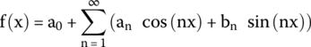
where:

- n = 1, 2, 3, …
18.2.2 Fourier transform
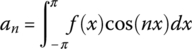
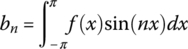
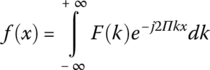
The Fourier transform of the function f(x) can be expressed as shown in Equation (18.2), and the inverse Fourier transform is shown in Equation (18.3).
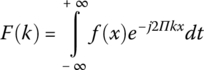
where:
 .
.
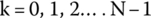
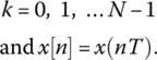
18.2.3 Discrete Fourier transform
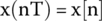
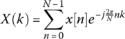
The discrete Fourier transform (DFT) of a discrete‐time signal x(nT) is given by Equation (18.4).
where:
If we let ![]() , then Equation (18.4) can be rewritten as Equation (18.5).
, then Equation (18.4) can be rewritten as Equation (18.5).
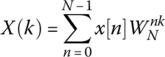
where:
- x[n] = input
- X[k] = frequency bins
- W = twiddle factors.
Therefore, for N samples of x, we have N frequencies (frequency bins) representing the signal, and each frequency bin can be calculated, as shown in Equation (18.5).
From Table 18.1, it is clear that the DFT requires N*N complex multiplications and (N − 1)*N complex additions.
Table 18.1 DFT calculation for every frequency bin
| X(0) = x[0]WN0 + x[1]WN0*1 + … + x[N − 1]WN0*(N−1) |
| X(1) = x[0]WN0 + x[1]WN1*1 + … + x[N − 1]WN1*(N−1) |
| : |
| X(k) = x[0]WN0 + x[1]WNk*1 + … + x[N − 1]WNk*(N−1) |
| : |
| X(N − 1) = x[0]WN0 + x[1]WN (N−1)*1 + … + x[N − 1]WN (N−1)(N−1) |
18.2.4 Fast Fourier transform
A large amount of work has been devoted to reducing the computation time of a DFT. This has led to efficient algorithms known as fast Fourier transforms. In this section, the algorithm known as Radix 2 FFT is developed.
18.2.4.1 Splitting the DFT into two DFTs
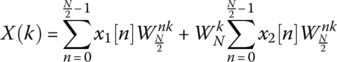
By manipulating the twiddle factor W, as shown here and in Figure 18.1, Equation (18.5) can be rewritten as shown in Equation (18.6).
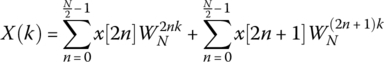
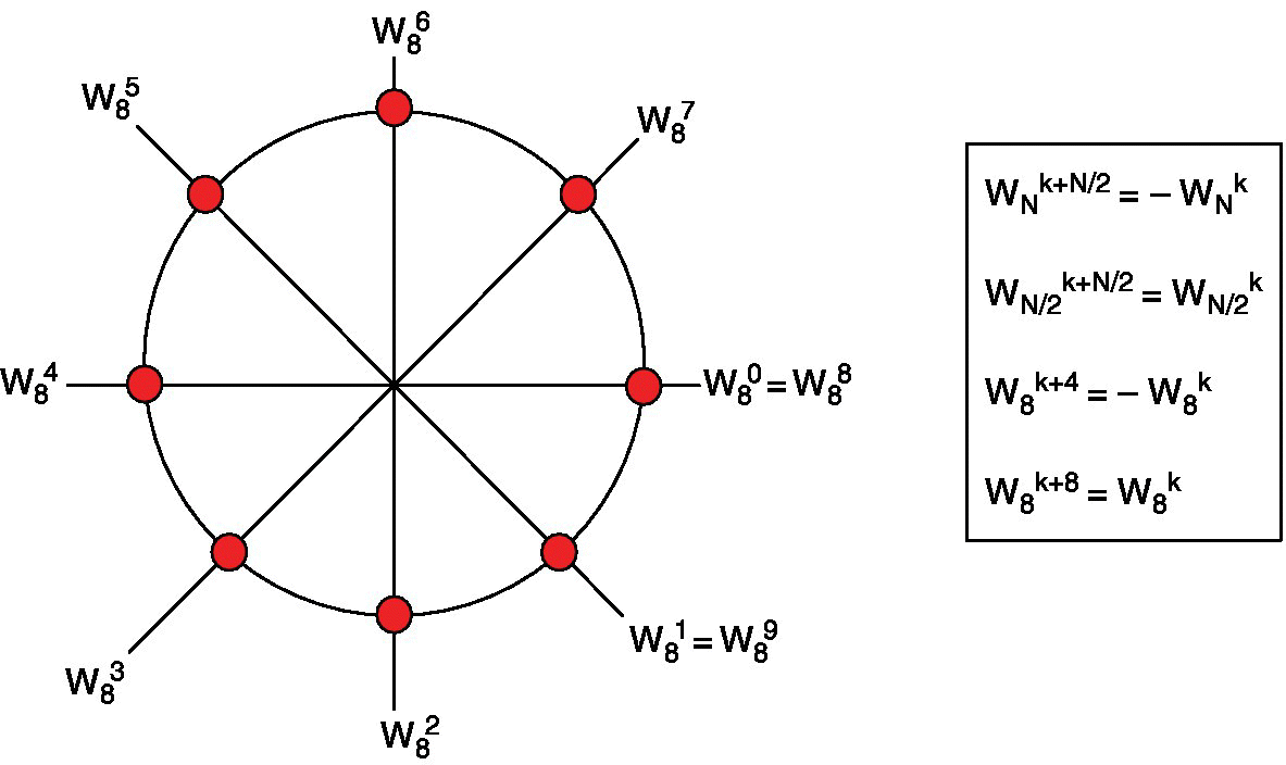
Figure 18.1 Twiddle factors for N = 8.
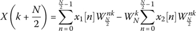
Replacing ![]() , x[2n] by x1[n] and
, x[2n] by x1[n] and ![]() , Equation (18.6) can be rewritten as shown in Equation (18.7).
, Equation (18.6) can be rewritten as shown in Equation (18.7).
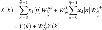
This shows that an N‐point DFT can be divided into two ![]() ‐point DFTs, Y(k) and Z(k), operating on the even and odd samples, respectively.
‐point DFTs, Y(k) and Z(k), operating on the even and odd samples, respectively.
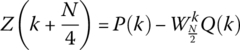
18.2.4.2 Exploiting the periodicity and symmetry of the twiddle factors
By exploiting the symmetry and periodicity of the twiddle factors, as shown here and illustrated in Figure 18.1, pairs of DFTs ![]() can be grouped together, as they share the same twiddle factors and therefore will reduce the number of calculations; see Equations (18.7) and (18.8).
can be grouped together, as they share the same twiddle factors and therefore will reduce the number of calculations; see Equations (18.7) and (18.8).
- Symmetry:

- Periodicity:
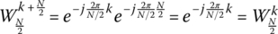 .
.

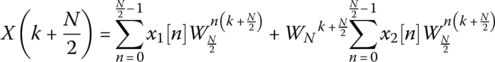
Using the periodicity, the pair of DFTs can be rewritten as shown in Equations (18.9) and (18.10):
Equations (18.9) and (18.10) can be rewritten as Equations (18.11) and (18.12).
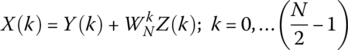
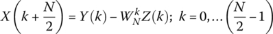
where Y(k) and Z(k) can be considered as two ![]() DFTs. By using the same process as shown in this section, Y(k) and Z(k) can be expressed as shown in Equations (18.13) to (18.16).
DFTs. By using the same process as shown in this section, Y(k) and Z(k) can be expressed as shown in Equations (18.13) to (18.16).
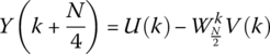
The process continues until 2‐point DFTs are reached. This is known as the decimation in time (DIT) Radix 2 FFT, as illustrated in Figure 18.2.
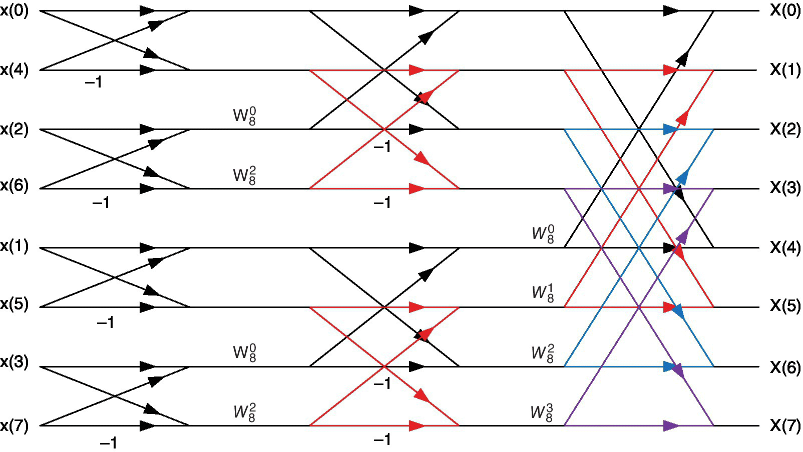
Figure 18.2 Decimation in time (DIT) Radix 2 FFT.
Note that input data need to be out of order (e.g. 0, 4, 2, 6, 1, 5, 3, 7, for an 8‐point FFT), and therefore the original data have to be reordered. This can be done by using a bit reversal since, when the binary representation of an index is reversed, it will lead to the correct value; see Figure 18.3. Reordering the input data of Figure 18.2 will lead to the decimation in frequency (DIF). However, the reordering should be performed at the end of the FFT; see Figure 18.4.
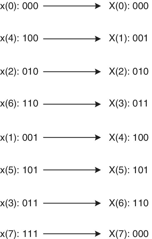
Figure 18.3 Bit reversal.
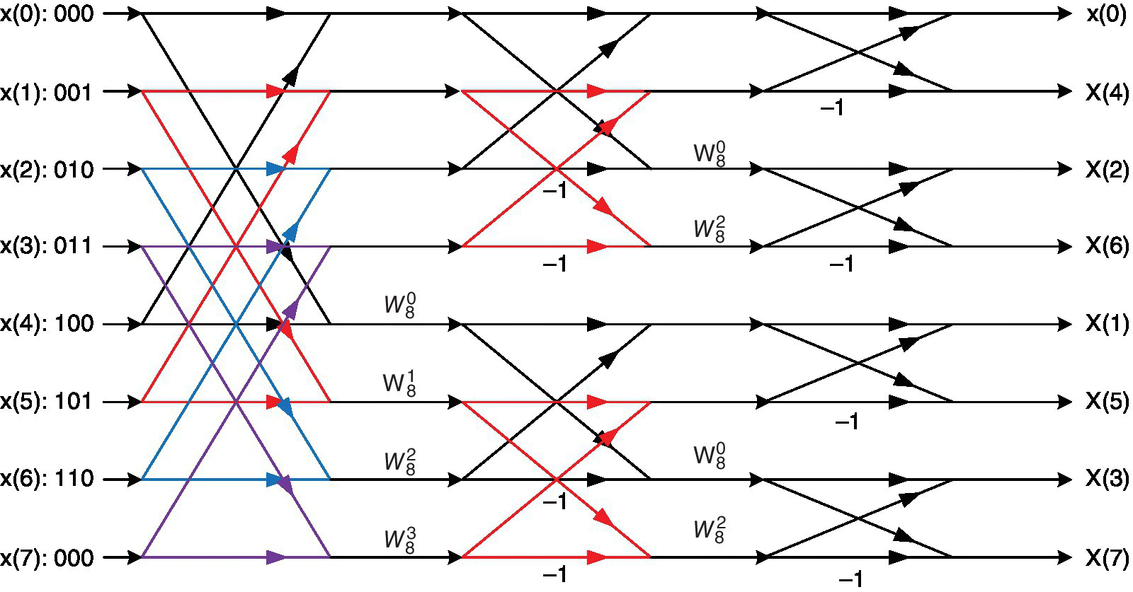
Figure 18.4 Decimation in frequency (DIF) Radix 2 FFT.
18.3 FFT implementation
To implement the FFT as illustrated in Figure 18.2, a few observations should be made:
- For an N‐point FFT, there are log2N stages. For N = 8, there will be three stages; see Figure 18.5.
- There are N/2stage blocks per stage.
- There are 2stage−1 butterflies per block.
- The difference in indices for each butterfly is the same in each block within a stage.
- The difference in indices for each butterfly in a group is twice that of the previous stage. Within Stage 1, there is a difference in indices of 1.
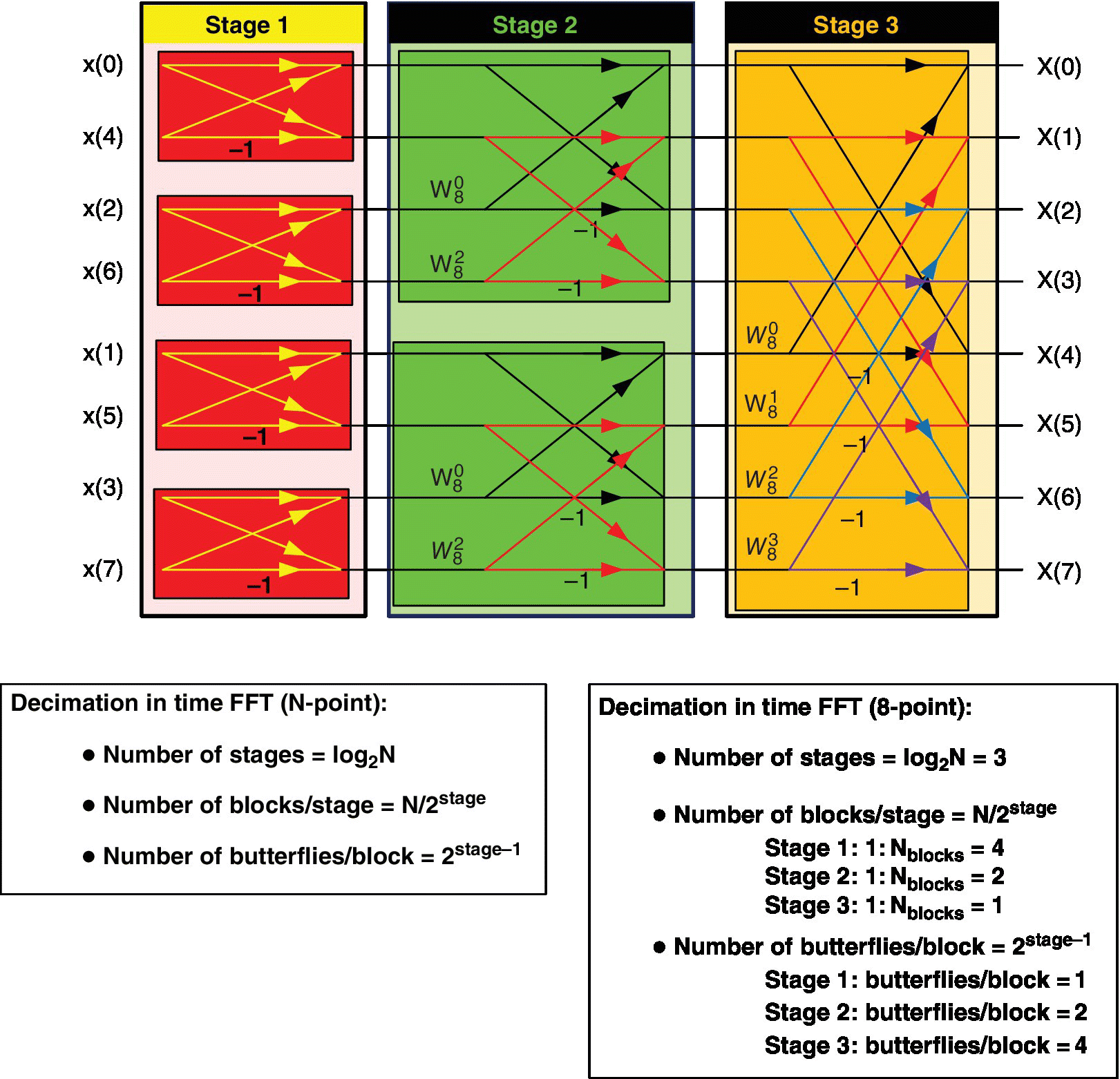
Figure 18.5 Diagram of DIT Radix 2 FFT used for the implementation.
To implement the inner loop (butterfly), let’s calculate the outputs A and B of the butterfly, as shown in Figure 18.6, and derive the C code.
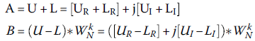
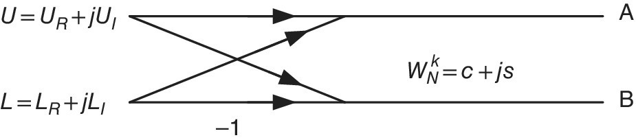
Figure 18.6 Flow graph of a butterfly.
Let’s simplify Equations A and B by assuming:
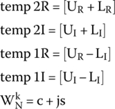
These will lead to:
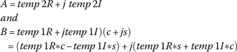
This can be implemented in C language by the C code shown in Figure 18.7. The complete implementation will require the calculations of each butterfly in each block starting from Stage 1 to the last stage. These can be performed by three loops, as shown in Figure 18.8.
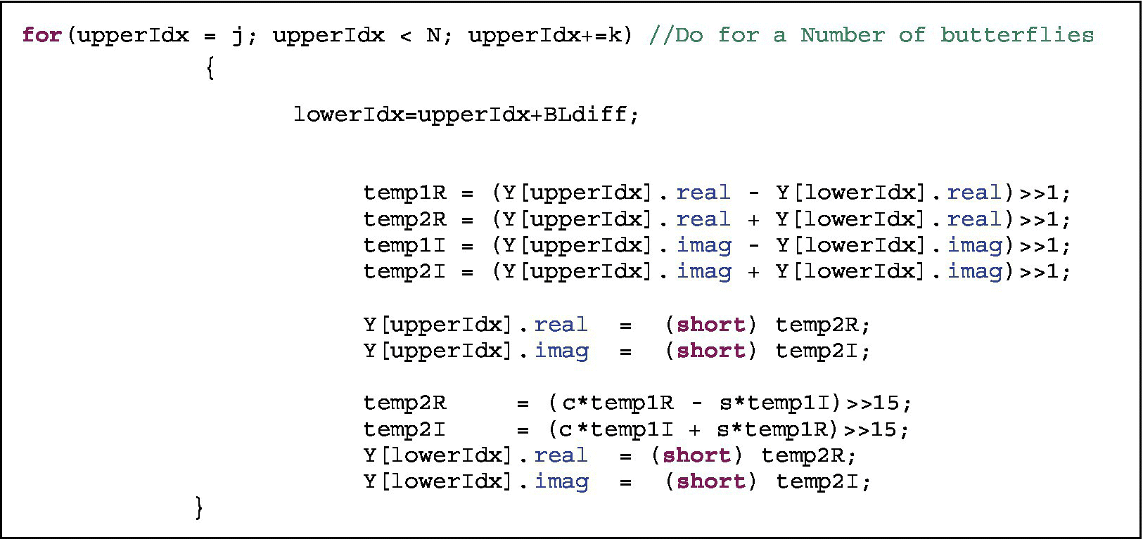
Figure 18.7 Implementation of the butterfly.
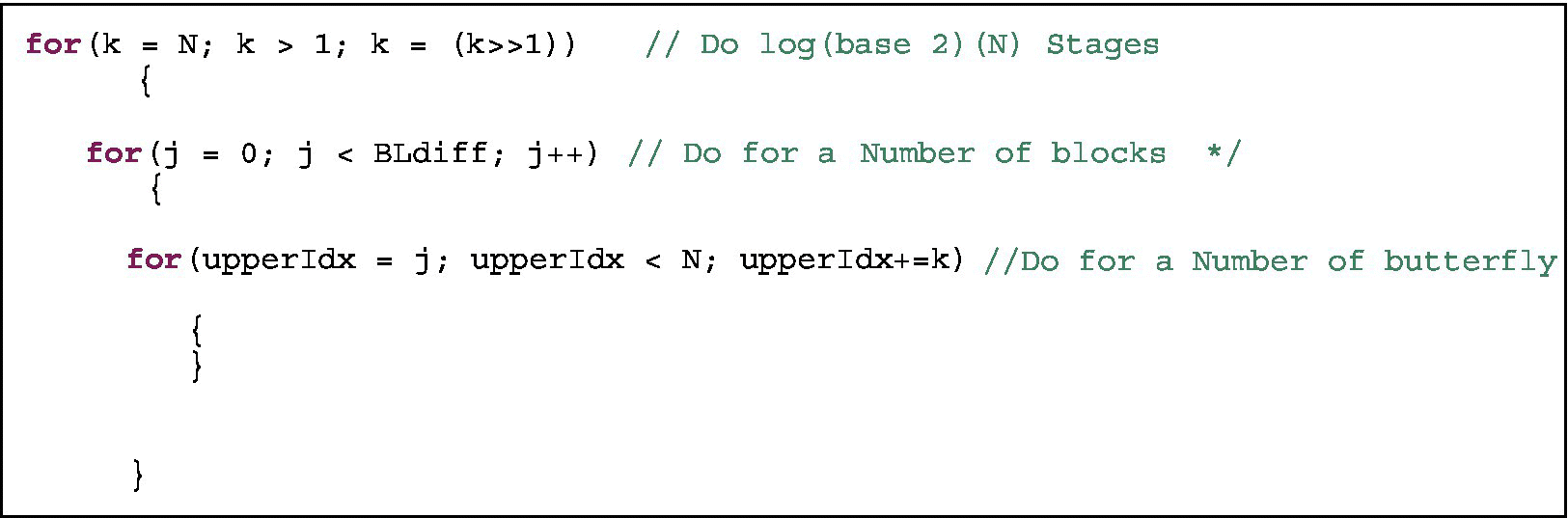
Figure 18.8 Main loops for implementing a Radix 2 FFT.
18.4 Laboratory experiment
18.4.1 Part 1: Implementation of DIF FFT
Files location:
- Chapter_18_CodeFFT_in_C
- Project: FFT_in_C.
In this laboratory experiment, a signal composed of two sinewaves is generated (this can be modified to add more sinewaves) and an FFT is performed on this signal, as shown in Figure 18.9.
- Step 1. Open the FFT_in_C project and check the tools used for this project, as shown in Figures 18.10 and 18.11. Rebuild the project, compile, load and run the code.
- Step 2. Display the signal and its FFT.
Figure 18.9 Tasks to perform.
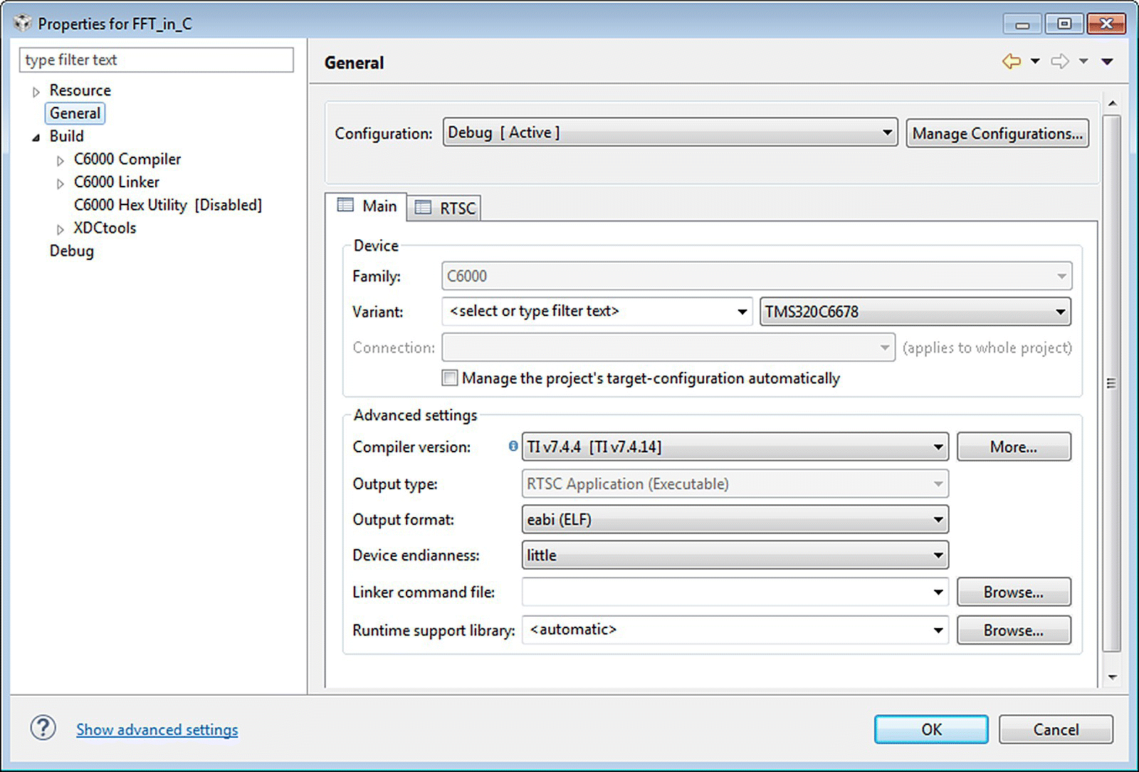
Figure 18.10 General configuration used.
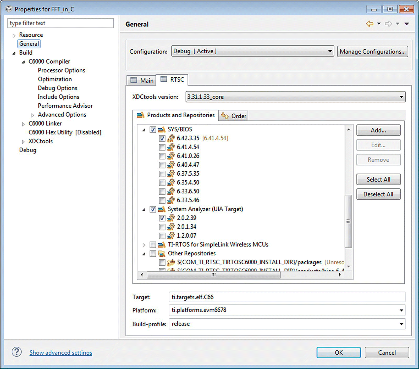
Figure 18.11 Real‐Time Software Components (RTSC) tools used.
Pause the program after running it for a few seconds. Explore the code for generating the sinewaves; see Figure 18.12. Watch the variable where the data are stored (buffer1[i] = sinegen() ) and open the graph window to display the data, as shown in Figure 18.13. Display the input data (as shown in Figure 18.15) by using buffer1 and the buffer property, as shown in Figures 18.13 and 18.14. Finally, display the FFT of the signal (as shown in Figure 18.18) by using the magg buffer and the buffer proprieties shown in Figures 18.16 and 18.17, respectively.
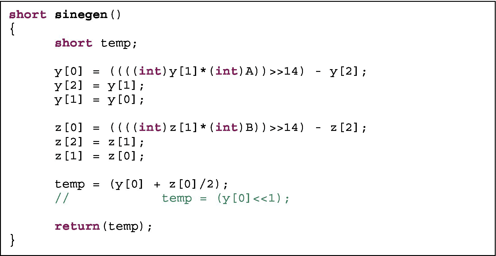
Figure 18.12 Code for generating sinewaves.
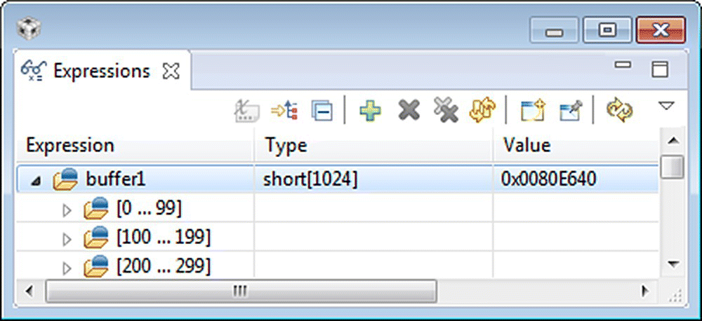
Figure 18.13 Buffer holding the input data.
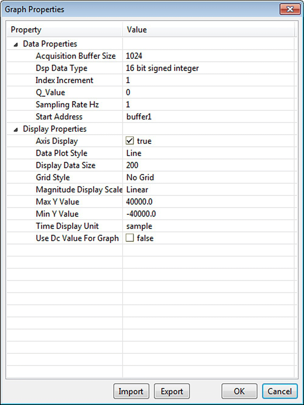
Figure 18.14 Graph properties used (Display_Time.graphProp).
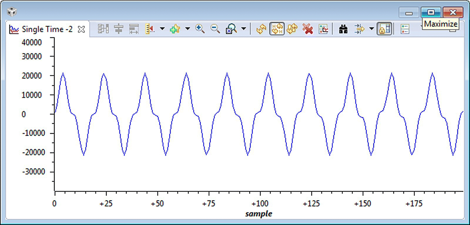
Figure 18.15 Display of the input data.
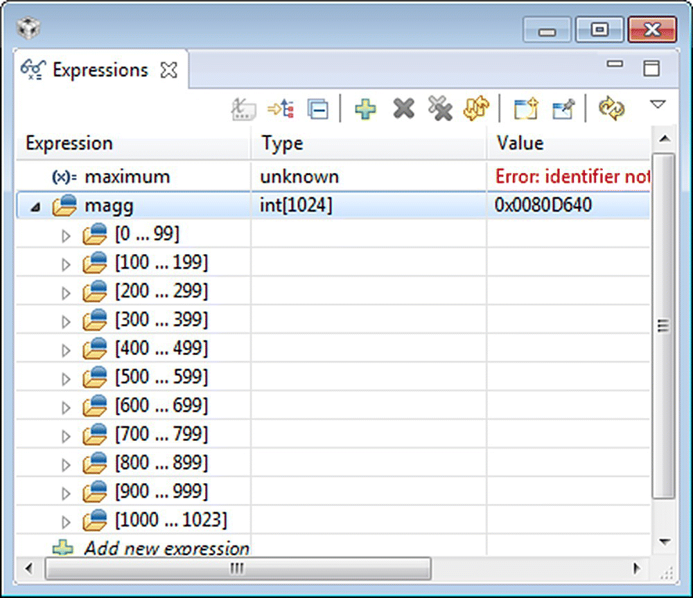
Figure 18.16 Buffer holding the magnitude magg.
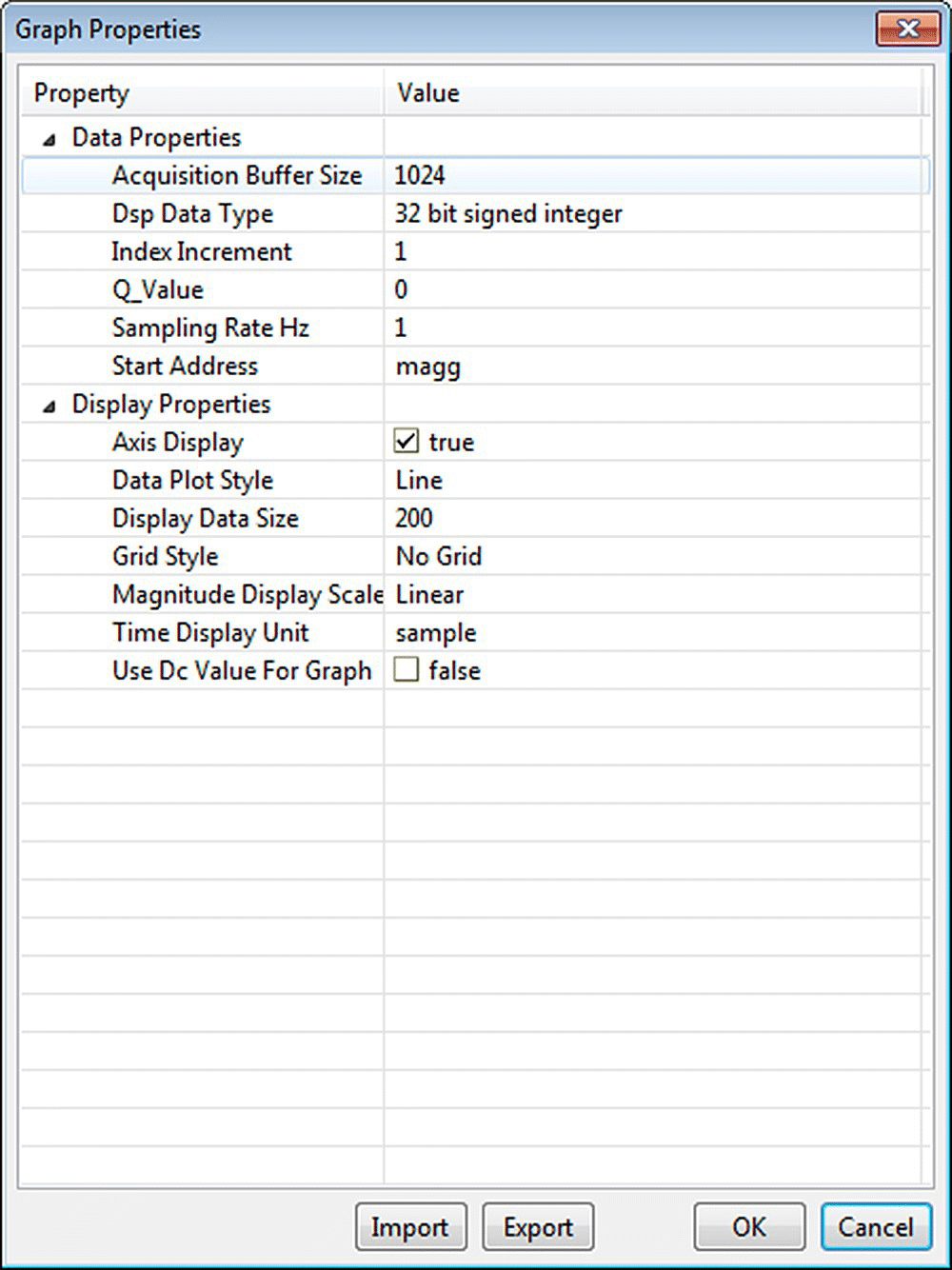
Figure 18.17 Graph properties.
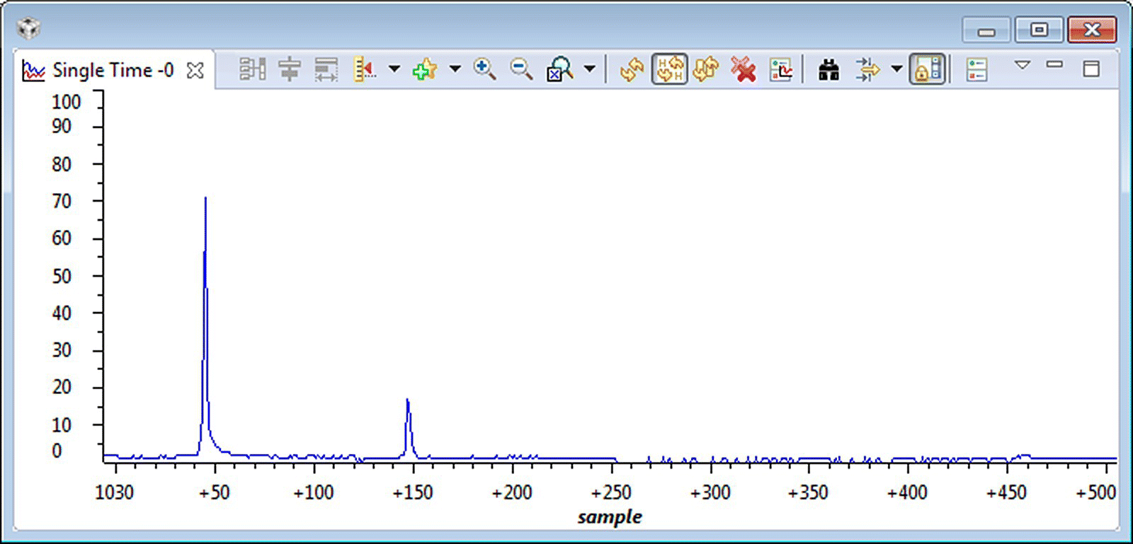
Figure 18.18 FFT display.
18.4.2 Part 2: Using ping‐pong EDMA
Files location:
- Chapter_18_CodeFFT_in_C_EDMA.
In this laboratory session, the EDMA copies data from a buffer (SrcPing) to another buffer DstPing. When the copy is completed, a callback function (cbckFunc) is called to instruct the EDMA to start another transfer of data from SrcPing to a DstPong buffer, and do an FFT, calculate the magnitude and extract the highest frequency bins (see Figure 18.19).
- Step 1. Open the project FFT_EDMA, rebuild it and load it.
- Step 2. Explore the main.c file. Notice that two sinewaves with two different frequencies and magnitudes are generated so that they can be distinguished when displayed. One can experiment with different frequencies and magnitudes (see the sinegen() function).
- Step 3. Set a breakpoint at the end of the call_magnitude() function.
- Step 4. Open a graph window and import Display_Timemagg.graphProp to display the content of the input data stored in the magg array; see Figure 18.20.
- Step 5. Run and observe the output graph; see Figure 18.21.
- Step 6. Now that the data are correct, let’s explore the magnitude of the FFT of the data stored in magg1. Open a graph window, and import Display_FFTmagg1.graphProp to display the content of the FFT magnitude stored in the magg1 array (see Figure 18.22; for the FFT output, see Figure 18.23). The code is located in the main.c file.
- Step 7. Repeat Step 6 to display the FFT of the data in magg2 (see Figures 18.24 and 18.25). The graph properties for displaying magg2 are located in Display_FFTmagg2.graphProp.
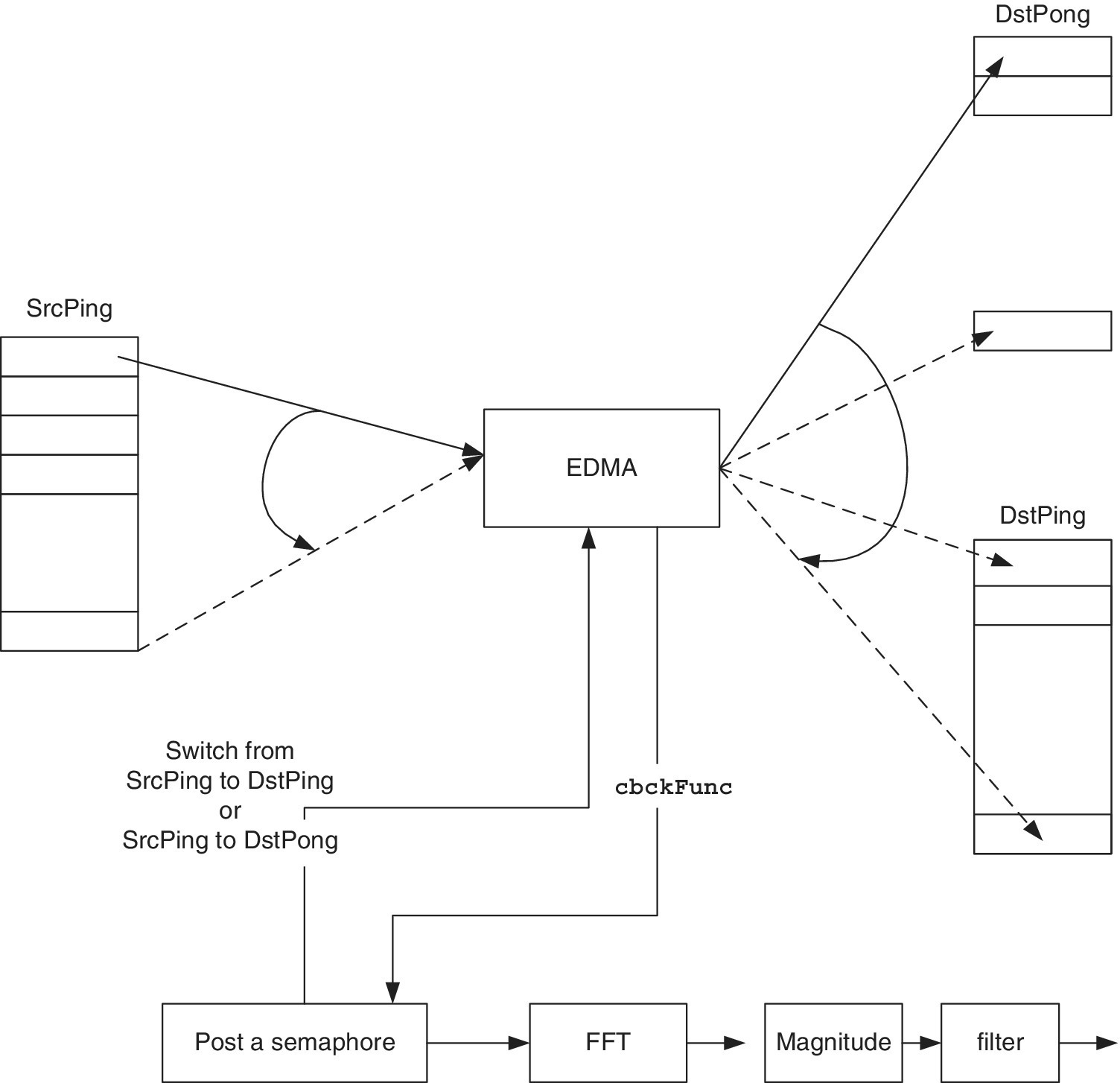
Figure 18.19 EDMA ping‐pong.

Figure 18.20 Properties for displaying the input data in the array magg.
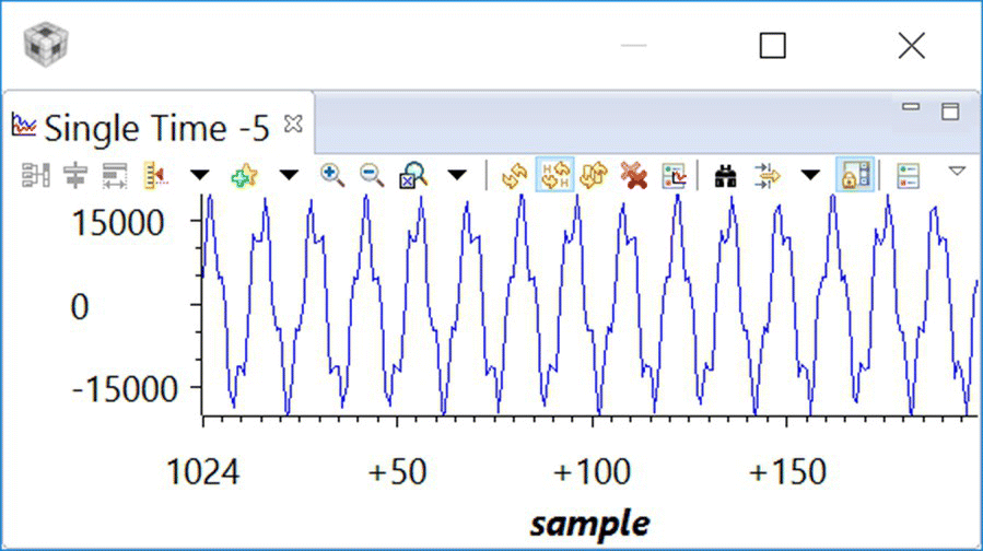
Figure 18.21 Display output.
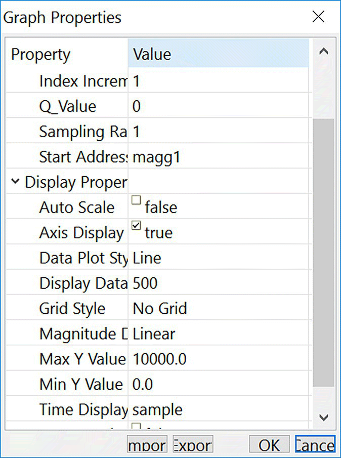
Figure 18.22 Properties for displaying the input data in the array magg1.
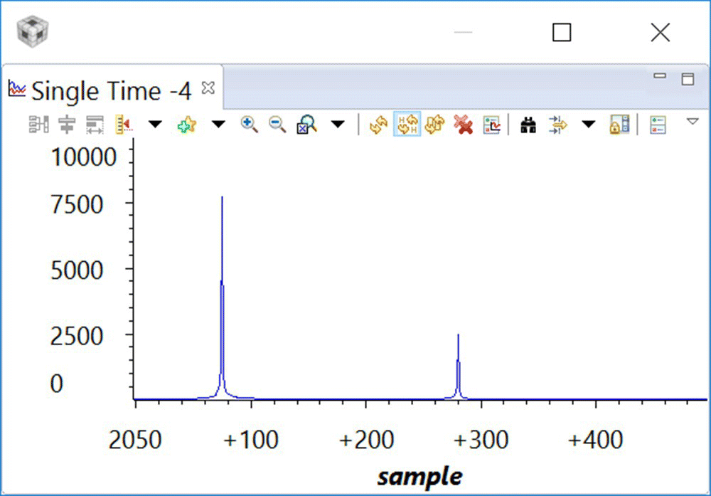
Figure 18.23 FFT magnitude display of data in dstPong.
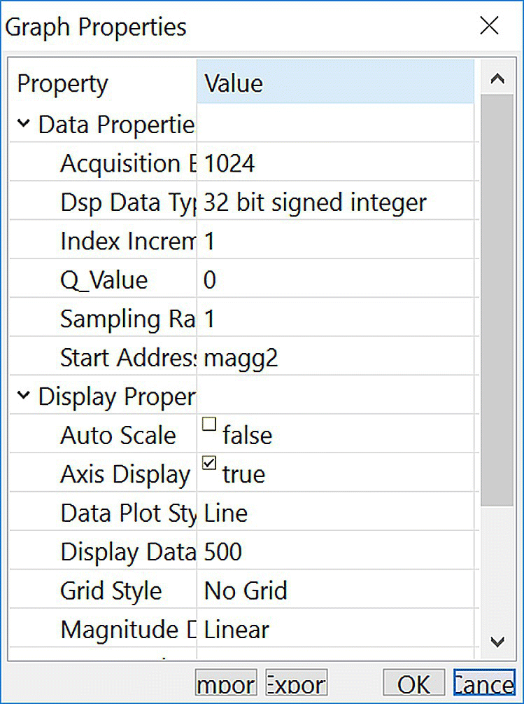
Figure 18.24 Properties for displaying the input data in the array magg2.
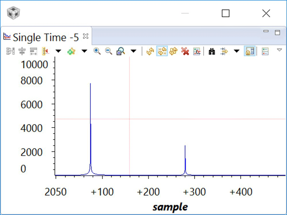
Figure 18.25 FFT magnitude display of data in dstPing.
18.5 Conclusion
In this chapter, the FFT Radix 2 has been studied, and a detailed implementation in C language has been provided. The implementation also includes using the EDMA to increase the performance.
References
- 1 J. W. Cooley and J. W. Tukey, An algorithm for the machine calculation of complex Fourier series, Mathematics of Computation, vol. 19, pp. 297–301, 1965.
- 2 I. J. Good, The interaction algorithm and practical Fourier analysis, Journal of the Royal Statistical Society, vol. 20, no. 2, pp. 361–372, 1958.
- 3 R. Yavne, An economical method for calculating the discrete Fourier transform, in AFIPS Fall Joint Computer Conference, Part I, San Francisco, CA, 1968.