
Chapter 1
Well-Being as a Multidimensional Phenomenon
1.1 Introduction
The choice of income as the only attribute or dimension of well-being of a population is inappropriate since it ignores heterogeneity across individuals in many other dimensions of living conditions. Each dimension represents a particular aspect of life about which people care. Examples of such dimensions include health, literacy, and housing. A person's achievement in a dimension indicates the extent of his performance in the dimension, for instance, how healthy he is, how friendly he is, how much is his monthly income, and so on.
Only income-dependent well-being quantifiers assume that individuals with the same level of income are regarded as equally well-off irrespective of their positions in such nonincome dimensions. In their report, prepared for the Commission on the Measurement of Economic Performance and Social Progress, constituted under a French Government initiative, Stiglitz et al. (2009, p. 14) wrote “To define what wellbeing means, a multidimensional definition has to be used. Based on academic research and a number of concrete initiatives developed around the world, the Commission has identified the following key dimensions that should be taken into account. At least in principle, these dimensions should be considered simultaneously: (i) Material living standards (income, consumption and wealth); (ii) Health; (iii) Education; (iv) Personal activities including work; (v) Political voice and governance; (vi) Social connections and relationships; (vii) Environment (present and future conditions); (viii) Insecurity, of an economic as well as a physical nature. All these dimensions shape people's wellbeing, and yet many of them are missed by conventional income measures.”
The need for analysis of well-being from multidimensional perspectives has also been argued in many contributions to the literature, including those of Rawls (1971); Kolm (1977); Townsend (1979); Streeten (1981); Atkinson and Bourguignon (1982); Sen (1985); Stewart (1985); Doyal and Gough (1991); Ramsay (1992); Tsui (1995); Cummins (1996); Ravallion (1996); Brandolini and D'Alessio (1998); Narayan (2000); Nussbaum (2000); Osberg and Sharpe (2002); Atkinson (2003); Bourguignon and Chakravarty (2003); Savaglio (2006a,b); Weymark (2006); Thorbecke (2008), Lasso de la Vega et al. (2009), Fleurbaey and Blanchet (2013); Aaberge and Brandolini (2015), Alkire et al. (2015); Duclos and Tiberti (2016).1
Nonmonetary dimensions of well-being are not unambiguously perfectly correlated with income. Consider a situation where, in some municipality of a developing country, there is a suboptimal supply of a local public good, say, mosquito control program. A person with a high income may not be able to trade off his income to improve his position in this nonmarketed, nonincome dimension of well-being (see Chakravarty and Lugo, 2016 and Decancq and Schokkaert, 2016).
In the capability-functioning approach, the notion of human well-being is intrinsically multidimensional (Sen, 1985, 1992; Sen and Nussbaum, 1993; Nussbaum, 2000; Pogge, 2002; Robeyns, 2009). Following John Stuart Mill, Adam Smith, and Aristotle, in the last 30 years or so, it has been reinterpreted and popularized by Sen in a series of contributions. In this approach, the traditional notions of commodity and utility are replaced respectively with functioning and capability.
Any kind of activity done or a state acquired by a person and a characteristic related to full description of the person can be regarded as a functioning. Examples include being well nourished, being healthy, being educated, and interaction with friends. Such a list can be formally represented by a vector of functionings. Capability may be defined as a set of functioning vectors that the person could have achieved.
It is possible to make a distinction between a good and functioning on the basis of operational difference. Of two persons, each owning a bicycle, the one who is physically handicapped cannot use the bike to go to the workplace as fast as the other person can. The bicycle is a good, but possessing the skill to ride it as per convenience is a functioning. This indicates that a functioning can be enacted by a good, but they are distinct concepts. Consequently, these two persons, each owning a bicycle, are not able to attain the same functioning (see Basu and López-Calva, 2011). Since the physically handicapped person, who lacks sufficient freedom to ride the bike as per desire, has a smaller capability set than the other person.
As Sen argued in several contributions, there is a clear distinction between starvation and fasting. Two persons may be in the same nutritional state, but one person fasting on some religious ground, say, is better off than the other person who is starving because he is poor. Since the former person has the freedom not to starve, his capability set is larger than that of the poor person (see also Fleurbaey, 2006a). Consequently, capabilities become closely related to freedom, opportunity, and favorable circumstances.2
Once the identification step, the selection of dimensions for determining human well-being, is over, at the next stage, we face the aggregation problem. The second step involves the construction of a comprehensive measure of well-being by aggregating the dimensional attainments of all individuals in the society. One simple approach can be dimension-by-dimension evaluation, resulting in a dashboard of dimensional metrics. A dashboard is a portfolio of dimension-wise well-being indictors (see Atkinson et al., 2002).3 A dashboard can be employed to monitor each dimension in separation. But the dashboard approach has some disadvantages as well. In the words of Stiglitz et al. (2009, p. 63), “dashboards suffer because of their heterogeneity, at least in the case of very large and eclectic ones, and most lackindications about…hierarchies among the indicators used. Furthermore, as communications instruments, one frequent criticism is that they lack what has made GDP a success: the powerful attraction of a single headline figure that allows simple comparisons of socio-economic performance over time or across countries.” The problem of heterogeneity across dimensional metrics can be taken care of by aggregating the dashboard-based measures into a composite index. The main disadvantage of this aggregation criterion is that it completely ignores relationships across dimensions. An alternative way to proceed toward building an all-inclusive measure of well-being is by clustering dimensional achievements across persons in terms of a real number. (See Ravallion, 2011, 2012, for a systematic comparison.)
The objective of this chapter is to evaluate how well a society is doing with respect to achievements of all the individuals in different dimensions. This is done using a social welfare function, which informs how well the society is doing when the distributions of dimensional achievements across different persons are considered. A social welfare function is regarded as a fundamental instrument in theoretical welfare economics. It has many policy-related applications. Examples include targeted equitable redistribution of income, assessment of environmental change, evaluation of health policy, cost–benefit analysis of a desired change, optimal provision of a public good, promoting goodness for future generations, assessment of legal affairs, and targeted poverty evaluation (see, among others, Balckorby et al., 2005; Adler, 2012, 2016; Boadway, 2016; Broome, 2016, and Weymark, 2016).
In order to make the chapter self-contained, in the next section, there will be a brief survey of univariate welfare measurement. Section 1.3 addresses the measurability problem of dimensional achievements. In other words, this section clearly investigates how achievements in different dimensions can be measured. Some basics for multivariate analysis of welfare are presented in Section 1.4. The concern of Section 1.5 is the dashboard approach to the evaluation of well-being. There will be a detailed scrutiny of alternative techniques for setting weights to individual dimensional metrics. In Section 1.6, there will be an analytical discussion on axioms for a multivariate welfare function. Each axiom is a representation of a property of a welfare measure that can be defended on its own merits. Often, axioms become helpful in narrowing down the choice of welfare measures. Section 1.7 studies welfare functions, including their information requirements, which have been proposed in the literature to assess multivariate distributions of well-being. Finally, Section 1.8 concludes the discussion.
1.2 Income as a Dimension of Well-Being and Some Related Aggregations
The measurement of multidimensional welfare originates from its univariate counterpart. In consequence, a short analytical treatment of one-dimensional welfare measurement at the outset will prepare the stage for our expositions in the following sections.
It is assumed before all else that no ambiguity arises with respect to definitions and related issues of the primary elements of the analysis. For instance, should the variable on which the analysis relies be income or expenditure? How is expenditure defined? What should be the reference period of observation of incomes/expenditure? How is the threshold income that represents a minimal standard of living determined (see Chapter 2)4? Generally, income data are collected at the household level. Income at the individual level can be obtained from the household income by employing an appropriate equivalence scale. (See Lewbel and Pendakur, 2008, for an excellent discussion on equivalence scale.) For simplicity of exposition, we assume that the unit of analysis is “individual.” If necessary, the study can be carried out at the household level.
For a population of size n, we denote an income distribution by a vector ![]() , where
, where ![]() is the nonnegative part
is the nonnegative part ![]() of the n-dimensional Euclidean space
of the n-dimensional Euclidean space ![]() with the origin deleted. More precisely,
with the origin deleted. More precisely, ![]() , where
, where ![]() is the n-coordinated vector of 1s. Here
is the n-coordinated vector of 1s. Here ![]() stands for the income of individual i in the population. Let
stands for the income of individual i in the population. Let ![]() be the positive part of
be the positive part of ![]() so that
so that ![]() . In consequence, the sets of all possible income distributions associated with
. In consequence, the sets of all possible income distributions associated with ![]() and
and ![]() become respectively
become respectively ![]() and
and ![]() , where
, where ![]() is a set of positive integers.
is a set of positive integers.
Unless stated, it will be assumed that ![]() represents the set of all possible income distributions. For the purpose at hand, we need to introduce some more notation. For all
represents the set of all possible income distributions. For the purpose at hand, we need to introduce some more notation. For all ![]() , for all
, for all ![]() ,
, ![]() (or, simply
(or, simply ![]() ) is the mean of
) is the mean of ![]() ,
,  . For all
 ![]() ,
, ![]() , let
, let ![]() denotethe nonincreasingly ordered permutation of u, that is,
denotethe nonincreasingly ordered permutation of u, that is, ![]() . Similarly, we write
. Similarly, we write ![]() for the nondecreasingly ordered permutation of
for the nondecreasingly ordered permutation of ![]() , that is,
, that is, ![]() . For all
. For all ![]() , for all
, for all ![]() , we write
, we write ![]() to mean that
to mean that ![]() for all
for all ![]() and
and ![]() . Hence,
. Hence, ![]() means that at least one income in
means that at least one income in ![]() is greater than the corresponding income in
is greater than the corresponding income in ![]() and no income in
and no income in ![]() is less than that in
is less than that in ![]() . The notation
. The notation ![]() will be used to mean that
will be used to mean that ![]() for all
for all ![]() .
.
An income-distribution-based social welfare function is a summary measure of the extent of well-being enjoyed by the individuals in a society, resulting from the spread of a given size of income among the individuals of the society. We denote this function by ![]() . Formally,
. Formally, ![]() . For any
. For any ![]() ,
, ![]() ,
, ![]() signifies the extent of welfare manifested by
signifies the extent of welfare manifested by ![]() . It is assumed beforehand that
. It is assumed beforehand that ![]() is continuous so that small changes in incomes will change welfare only marginally. Since it determines the standard of welfare, we can also refer to as a welfare standard.
is continuous so that small changes in incomes will change welfare only marginally. Since it determines the standard of welfare, we can also refer to as a welfare standard.
Next, we state certain desirable axioms for ![]() . The terms “axiom” and “postulate” will be used interchangeably because they are assumed without proof. Each axiom represents a particular value judgment, and it may not be verifiable by factual evidence. We will as well use the terms “property” and “principle” in place of axiom. Implicit under the choice of a welfare function
. The terms “axiom” and “postulate” will be used interchangeably because they are assumed without proof. Each axiom represents a particular value judgment, and it may not be verifiable by factual evidence. We will as well use the terms “property” and “principle” in place of axiom. Implicit under the choice of a welfare function ![]() is also acceptance of the axioms that are verified by
is also acceptance of the axioms that are verified by ![]() . Rawls (1971, p. 80) refers to the choice of a form
. Rawls (1971, p. 80) refers to the choice of a form ![]() as the index problem. Since our study of their multidimensional dittos will be extensive, here our discussion will be brief.
as the index problem. Since our study of their multidimensional dittos will be extensive, here our discussion will be brief.
- Symmetry: For all
 ,
,  ,
,  , where
  is any reordering of
  .
.
According to this postulate, welfare evaluation of the society remains unaffected if any two individuals swap their positions in the distribution. Equivalently, any feature other than income has no role in welfare assessment.
- Symmetry Axiom for Population: For all
 ,
,  ,
,  , where
  is the income vector in which each
  is repeated
  times,
  being any positive integer.
This property, introduced by Dalton (1920), requires ![]() to be expressed in terms of an average of the population size so that welfare judgment remains unchanged when the same population is pooled several times. It demonstrates neutrality property of the welfare standard
to be expressed in terms of an average of the population size so that welfare judgment remains unchanged when the same population is pooled several times. It demonstrates neutrality property of the welfare standard ![]() with respect to population size, indicating invariance of the standard under replications of the population. Consequently, the postulate becomes useful in performing comparisons of welfare across societies and of the same society over time, where the underlying population sizes are likely to differ.5
with respect to population size, indicating invariance of the standard under replications of the population. Consequently, the postulate becomes useful in performing comparisons of welfare across societies and of the same society over time, where the underlying population sizes are likely to differ.5
- Increasingness: For all
 , for all
  , if
, if  , then
  .
.
This property claims that if at least one person's income registers an increase, then the society moves to a better welfare position. An increasing welfare function indicates preferences for higher incomes; more income is preferred to less.
The final property we wish to introduce represents equity biasness of the welfare standard. Equity orientation in welfare evaluation can be materialized through a progressive transfer, an equitable redistribution of income. Formally, for all ![]() ,
, ![]() , we say that
, we say that ![]() is obtained from
is obtained from ![]() by a progressive transfer if for some i, j and c > 0
by a progressive transfer if for some i, j and c > 0 ![]() ,
, ![]() , and
, and ![]() for all
for all ![]() . That is, u is obtained from
. That is, u is obtained from ![]() by a transfer of c units of income from a person j to a person i who has lower income than j such that the transfer does not make j poorer than i and incomes of all other persons remain unaffected. Equivalently, we say that
by a transfer of c units of income from a person j to a person i who has lower income than j such that the transfer does not make j poorer than i and incomes of all other persons remain unaffected. Equivalently, we say that ![]() is obtained from
is obtained from ![]() by a regressive transfer.
by a regressive transfer.
- Pigou–Dalton Transfer: For all
 , for all
  , if,
, if,  is obtained from
  by a progressive transfer, then
  .
.
In words, welfare should increase under a progressive transfer.6 The Pigou–Dalton transfer principle, despite its limitations, is easy to understand and becomes equivalent to several seemingly unrelated conditions. Our multidimensional dominance properties that require welfare to rise when equitable redistributions occur bear similarities with these conditions. Consequently, a discussion on these conditions becomes justifiable.
Use of a numerical example will probably make the situation clearer. Consider the ordered income vectors ![]() and
and ![]() . Of these two ordered profiles, the former is obtained from the latter by a progressive transfer of 1 unit of income from the richest person to the poorest person. This transfer does not alter the rank orders of the individuals. That is why it is a rank-preserving progressive transfer. Equivalently, we can generate
. Of these two ordered profiles, the former is obtained from the latter by a progressive transfer of 1 unit of income from the richest person to the poorest person. This transfer does not alter the rank orders of the individuals. That is why it is a rank-preserving progressive transfer. Equivalently, we can generate ![]() by postmultiplying
by postmultiplying ![]() by some
by some ![]() bistochastic matrix.7 If we denote this bistochastic matrix by
bistochastic matrix.7 If we denote this bistochastic matrix by ![]() , then
, then

An alternative equivalent condition for executing the redistributive operation that takes us from ![]() to
to ![]() is to postmultiply the former by some
is to postmultiply the former by some ![]() Pigou–Dalton matrix.8 To see this more concretely, denote the underlying Pigou–Dalton matrix by
Pigou–Dalton matrix.8 To see this more concretely, denote the underlying Pigou–Dalton matrix by ![]() . Then
. Then

The particular Pigou–Dalton matrix T in (1.2) is the sum of ![]() times the
times the ![]() identity matrix and
identity matrix and ![]() times a
times a ![]() permutation matrix obtained by swapping the first and third entries in the first and third rows, respectively, of the identity matrix.
permutation matrix obtained by swapping the first and third entries in the first and third rows, respectively, of the identity matrix.
A graphical equivalence of the aforementioned three interchangeable statements is that ![]() Lorenz dominates
Lorenz dominates ![]() , which means that the Lorenz curve of the former in no place lies below that of the latter and lies above in some places (at least).9 In terms of welfare ranking, this is the same as the requirement that
, which means that the Lorenz curve of the former in no place lies below that of the latter and lies above in some places (at least).9 In terms of welfare ranking, this is the same as the requirement that ![]() , where
, where ![]() is any arbitrary strictly S-concave social welfare function.10
is any arbitrary strictly S-concave social welfare function.10
We now review three well-known examples of univariate social welfare functions. Since multidimensional translations of these functions will be explored in detail in one of the following sections, this brief study becomes rewarding. The first example we wish to scrutinize is the symmetric mean of order ![]() , which for any
, which for any ![]() and
and ![]() is defined as
is defined as

Since ![]() is undefined for
is undefined for ![]() if at least one income is nonpositive,
if at least one income is nonpositive, ![]() is chosen as its domain. The superscript
is chosen as its domain. The superscript ![]() in
in ![]() signifies sensitivity of the parameter
signifies sensitivity of the parameter ![]() to
to ![]() , and the subscript
, and the subscript ![]() is used to indicate that it corresponds to the Atkinson (1970) inequality index (see Chapter 2). For any
is used to indicate that it corresponds to the Atkinson (1970) inequality index (see Chapter 2). For any ![]() , the aggregation process invoked in
, the aggregation process invoked in ![]() is as follows. First, all incomes are transformed by taking their
is as follows. First, all incomes are transformed by taking their ![]() power. The transformation, defined by
power. The transformation, defined by ![]() power of a positive real number, employed on the average
power of a positive real number, employed on the average  gives us
 ![]() . This continuous, increasing, symmetric, and population-size-invariant welfare function demonstrates equity orientation (satisfaction of strict S-concavity) if and only if
. This continuous, increasing, symmetric, and population-size-invariant welfare function demonstrates equity orientation (satisfaction of strict S-concavity) if and only if ![]() . Adler (2012) suggested the use of this welfare standard for moral assessment of decisions that have significant social implications.
. Adler (2012) suggested the use of this welfare standard for moral assessment of decisions that have significant social implications.
For any income profile, an increase in the value of ![]() increases welfare. The reason behind this is that as the value of
increases welfare. The reason behind this is that as the value of ![]() decreases, higher weights are assigned to lower incomes in the aggregation. Since the assignment of higher weights to lower income holds for all
decreases, higher weights are assigned to lower incomes in the aggregation. Since the assignment of higher weights to lower income holds for all ![]() , a progressive income transfer will increase welfare by a larger amount, the lower the income of the recipient is. For
, a progressive income transfer will increase welfare by a larger amount, the lower the income of the recipient is. For ![]() ,
, ![]() becomes the harmonic mean. It reduces to the geometric mean if
becomes the harmonic mean. It reduces to the geometric mean if ![]() . As
. As ![]() ,
, ![]() approaches
approaches ![]() , the maximin welfare function (Rawls, 1971), a welfare standard that prioritize the worst-off individual. In other words, in this case, welfare ranking is decided by the income of the worst-off individual.
, the maximin welfare function (Rawls, 1971), a welfare standard that prioritize the worst-off individual. In other words, in this case, welfare ranking is decided by the income of the worst-off individual.
The second welfare function we choose is the Donaldson and Weymark (1980) well-known S-Gini welfare function, which for any ![]() and
and ![]() is defined as
is defined as

Given that incomes are nonincreasingly arranged, increasingness of the weight sequence ![]() , where
, where ![]() , ensures strict S-concavity (hence symmetry) of
, ensures strict S-concavity (hence symmetry) of ![]() . This continuous, increasing, and population-size-invariant welfare function possesses a simple disaggregation property. If each income is broken down into two components, say, salary income and interest income, and the ranks of the individuals in the two distributions are the same, then overall welfare is simply the sum of welfares from two component distributions (see Weymark, 1981). A higher value of
. This continuous, increasing, and population-size-invariant welfare function possesses a simple disaggregation property. If each income is broken down into two components, say, salary income and interest income, and the ranks of the individuals in the two distributions are the same, then overall welfare is simply the sum of welfares from two component distributions (see Weymark, 1981). A higher value of ![]() makes welfare standard more sensitive to lower incomes within a distribution. When the single parameter
makes welfare standard more sensitive to lower incomes within a distribution. When the single parameter ![]() increases unboundedly,
increases unboundedly, ![]() converges toward the maximin function. For
converges toward the maximin function. For ![]() ,
, ![]() becomes the one-dimensional Gini welfare function
becomes the one-dimensional Gini welfare function  , a weighted average of rank-ordered incomes, where the weights themselves are rank-dependent. It is also popularly known as the Gini mean (Fleurbaey and Maniquet, 2011). Foster et al. (2013a,b) refer to this as the Sen mean.11 It can alternatively be written as the expected value of the minimum of two randomly drawn incomes, where the random drawing is done with replacement. More precisely,
  . From this formulation of the Gini mean, it is evident that for any unequal
 ![]() , it is less than the ordinary mean
, it is less than the ordinary mean ![]() .
.
Pollak (1971) analyzed the family of exponential additive welfare functions, of which a simple symmetric representation is  , where
 ![]() and
and ![]() are arbitrary;
are arbitrary; ![]() is a parameter; and “exp” stands for the exponential function. This sign restriction on
is a parameter; and “exp” stands for the exponential function. This sign restriction on ![]() ensures that
ensures that ![]() is increasing and strictly S-concave. It indicates sensitivity to lower incomes in the population. This welfare standard fails to satisfy a common property of
is increasing and strictly S-concave. It indicates sensitivity to lower incomes in the population. This welfare standard fails to satisfy a common property of ![]() and
and ![]() ; if incomes are equal across individuals, welfare is judged by the equal income itself. However, the following function
; if incomes are equal across individuals, welfare is judged by the equal income itself. However, the following function

analyzed by Kolm (1976), which is related to ![]() via the continuous, increasing transformation
via the continuous, increasing transformation ![]() , fulfills this criterion. Consequently, they will rank two income vectors over the same population in the same way. This transformation also makes
, fulfills this criterion. Consequently, they will rank two income vectors over the same population in the same way. This transformation also makes ![]() fulfill the symmetry postulate for population and preserves strict S-concavity (hence, symmetry) of
fulfill the symmetry postulate for population and preserves strict S-concavity (hence, symmetry) of ![]() . As
. As ![]() is increased limitlessly,
is increased limitlessly, ![]() becomes closer and closer to the maximin function.
becomes closer and closer to the maximin function.
We conclude this section by noting that while ![]() is linear homogeneous,
is linear homogeneous, ![]() is unit translatable. According to linear homogeneity, an equiproportionate variation in all incomes will change welfare by the same proportion. In contrast, unit translatability claims that an equal absolute change in all incomes will change welfare by the absolute amount itself.12 An example of a linear homogeneous and unit translatable welfare function is
is unit translatable. According to linear homogeneity, an equiproportionate variation in all incomes will change welfare by the same proportion. In contrast, unit translatability claims that an equal absolute change in all incomes will change welfare by the absolute amount itself.12 An example of a linear homogeneous and unit translatable welfare function is ![]() .
.
1.3 Scales of Measurement: A Brief Exposition
Measurement scales specify the ways in which we can classify the variables. For each class of variables, some relevant operations can be executed so that the transmissions do not generate any loss of information (Stevens, 1946).
To grasp the issue in greater detail, suppose that w, a person's weight, is measured in kilograms. By multiplying w by 1000, we can alternatively express this weight as ![]() grams. This process of conversion of weight from kilograms to grams, by multiplying by the ratio
grams. This process of conversion of weight from kilograms to grams, by multiplying by the ratio ![]() , which does not lead to any loss of information on the person's weight, is admitted by indicators of ratio scale. Formally, an indicator
, which does not lead to any loss of information on the person's weight, is admitted by indicators of ratio scale. Formally, an indicator ![]() is said to measurable on ratio scale if there is perfect substitutability between its value
is said to measurable on ratio scale if there is perfect substitutability between its value ![]() and
and ![]() , where
, where ![]() is a constant. For ratio-scale indicators, there is a natural “zero”; 0 weight means “no weight,” whether it is expressed in kilograms or grams. A second example of a ratio-scale dimension is height.
is a constant. For ratio-scale indicators, there is a natural “zero”; 0 weight means “no weight,” whether it is expressed in kilograms or grams. A second example of a ratio-scale dimension is height.
An interval scale refers to a measurement in which the difference between two values can be meaningfully compared. To understand this, consider the vector of temperatures ![]() expressed in degree centigrade. These temperatures can equivalently be specified in degree Fahrenheit as
expressed in degree centigrade. These temperatures can equivalently be specified in degree Fahrenheit as ![]() . The difference between the temperatures 20 and 10 degrees is the same as that between 40 and 30 in
. The difference between the temperatures 20 and 10 degrees is the same as that between 40 and 30 in ![]() . Similarly, there is a common difference between 68 and 50 and between 104 and 86 in
. Similarly, there is a common difference between 68 and 50 and between 104 and 86 in ![]() . The two common differences are different because the temperatures in Centigrade (C) and Fahrenheit scales (F) are connected by the one-to-one transformation
. The two common differences are different because the temperatures in Centigrade (C) and Fahrenheit scales (F) are connected by the one-to-one transformation ![]() . But a temperature of 30 °C cannot be regarded as thrice as that of 10 °C. However, for a ratio-scale variable, this is meaningful. Further, there is no natural “zero” in interval scale. A 0 degree temperature does not indicate absence of heat, irrespective of whether it is stated in Centigrade or in Fahrenheit. More generally, an indicator
. But a temperature of 30 °C cannot be regarded as thrice as that of 10 °C. However, for a ratio-scale variable, this is meaningful. Further, there is no natural “zero” in interval scale. A 0 degree temperature does not indicate absence of heat, irrespective of whether it is stated in Centigrade or in Fahrenheit. More generally, an indicator ![]() is said to be measurable on interval scale if its value
is said to be measurable on interval scale if its value ![]() can be perfectly substituted by
can be perfectly substituted by ![]() , where
, where ![]() and a are constants. A transformation of this type is called an affine transformation. A second example of an interval-scale indicator is intelligent quotient score. Variables measurable on ratio and interval scales exhaust the class of cardinally measurable variables.
and a are constants. A transformation of this type is called an affine transformation. A second example of an interval-scale indicator is intelligent quotient score. Variables measurable on ratio and interval scales exhaust the class of cardinally measurable variables.
A variable representing two or more mutually exclusive but not ranked categories is known as a categorical or a nominal variable. For example, we can identify female and male workers in an organization as type I and type II categories of workers. But we can as well label male workers as type I and female workers as type II workers. More precisely, there is well-defined division of the categories. Another example of a categorical variable can be labeling of subgroups of population formed by some socioeconomic characteristic, say, race, region, and religion. In contrast, for an ordinally significant variable, there is a well-defined ordering rule of the categories. For instance, we can classify individuals in a society with respect to their educational attainments into five categories: illiterate, having knowledge just to read and write in some language, elementary school graduate, high school graduate, and college graduate. We can assign the numbers 0, 1, 2, 3, and 4 to these levels of educational attainments to rank them in increasing order. Here the difference between 1 and 0 is not the same as that between 3 and 2. We can alternatively rank these categories using the numbers 0, 1, 4, 9, and 16. These numbers are obtained by squaring the previously assigned numbers 0, 1, 2, 3, and 4. Consequently, accreditation of numbers is arbitrary; the only restriction is that a higher number should be attributed to a higher category so that ranking remains preserved. Hence, the category “college graduate” should always be assigned a higher number compared to the category “high school graduate.” More generally, a transformation of the type ![]() , where f is increasing, will keep ordering of transformed values
, where f is increasing, will keep ordering of transformed values ![]() of initial numbers
of initial numbers ![]() of the variable l unaltered. Hence, any increasing function f can be regarded as an admissible transformation here. A second example of a variable with ordinal significance is “self-reported health condition,” judged in terms of some health level categories, ranked in increasing order of better conditions. (See, for example, Allison and Foster (2004).) Such variables are also known as qualitative variables.13
of the variable l unaltered. Hence, any increasing function f can be regarded as an admissible transformation here. A second example of a variable with ordinal significance is “self-reported health condition,” judged in terms of some health level categories, ranked in increasing order of better conditions. (See, for example, Allison and Foster (2004).) Such variables are also known as qualitative variables.13
1.4 Preliminaries for Multidimensional Welfare Analysis
Before we discuss the relevance of our presentation in the earlier section in the present context, let us introduce some preliminaries. We consider a society consisting of ![]() individuals. Assume that there are d dimensions of well-being. The set of well-being dimensions
individuals. Assume that there are d dimensions of well-being. The set of well-being dimensions ![]() is denoted by Q. The number of dimensions d is assumed to be exogenously given. Let
is denoted by Q. The number of dimensions d is assumed to be exogenously given. Let ![]() stand for person i's achievement in dimension j. It is assumed at the beginning that we have complete information on these primary elements of analysis. (For social evaluations based on individuals' consumption patterns, see Jorgenson and Slesnick, 1984.)
stand for person i's achievement in dimension j. It is assumed at the beginning that we have complete information on these primary elements of analysis. (For social evaluations based on individuals' consumption patterns, see Jorgenson and Slesnick, 1984.)
Since ![]() and
and ![]() are arbitrary, distribution of dimensional achievements in the population is represented by an
are arbitrary, distribution of dimensional achievements in the population is represented by an ![]() achievement matrix X whose
achievement matrix X whose ![]() entry is
entry is ![]() . The jth column of X, denoted by
. The jth column of X, denoted by ![]() , shows the distribution of the total achievement
, shows the distribution of the total achievement  in dimension j across n individuals. For any
 ![]() ,
, ![]() stands for the mean of the distribution
stands for the mean of the distribution ![]() . The ith row of X, denoted by
. The ith row of X, denoted by ![]() , is an array of person i's achievements in different dimensions. We say that
, is an array of person i's achievements in different dimensions. We say that ![]() represents person i's achievement profile in X. We will often use the terms “social matrix,” “distribution matrix,” and “social distribution” for an achievement matrix.
represents person i's achievement profile in X. We will often use the terms “social matrix,” “distribution matrix,” and “social distribution” for an achievement matrix.
The matrix ![]() is an arbitrary element of the set
is an arbitrary element of the set ![]() , the set of all
, the set of all ![]() achievement matrices with nonnegative achievements in each dimension. Let
achievement matrices with nonnegative achievements in each dimension. Let ![]() . In words,
. In words, ![]() is a set of achievement matrices over the population consisting of
is a set of achievement matrices over the population consisting of ![]() individuals, and the mean of achievements in each dimension is positive. Finally, define
individuals, and the mean of achievements in each dimension is positive. Finally, define ![]() as a set of achievement matrices over the population with size
as a set of achievement matrices over the population with size ![]() such that for each individual, all dimensional achievements are positive. Formally,
such that for each individual, all dimensional achievements are positive. Formally, ![]() . Evidently,
. Evidently, ![]() ,
, ![]() , and
, and ![]() can be regarded as multidimensional analogs of
can be regarded as multidimensional analogs of ![]() ,
, ![]() , and
, and ![]() , respectively. Let
, respectively. Let ![]() stand for the set of all possible achievement matrices corresponding to
stand for the set of all possible achievement matrices corresponding to ![]() , that is,
, that is, ![]() . The corresponding sets of all achievement matrices associated with
. The corresponding sets of all achievement matrices associated with ![]() and
and ![]() that parallel to
that parallel to ![]() are denoted respectively by
are denoted respectively by ![]() and
and ![]() . Barring anything specified, our presentation in the following sections will be made in terms of an arbitrary
. Barring anything specified, our presentation in the following sections will be made in terms of an arbitrary ![]() .
.
For illustrative purpose, let us assume that there are three dimensions of well-being, namely daily energy consumption in calories by an adult male,14 per capita income, and life expectancy, measured respectively in dollars and years. With these three dimensions of well-being, we consider the following matrix ![]() as an example of an achievement matrix in a four-person economy:
as an example of an achievement matrix in a four-person economy:

The first entry in row i of ![]() indicates person i's daily calorie intake. On the other hand, the second and third entries of the row specify respectively the person's life expectancy and income.
indicates person i's daily calorie intake. On the other hand, the second and third entries of the row specify respectively the person's life expectancy and income.
All our axioms in this chapter will be stated using a social welfare function W, a real-valued function defined on the set of achievement matrices. Formally, ![]() , where for any
, where for any ![]() ,
, ![]() ,
, ![]() indicates the level of well-being associated with the distributions of totals of achievements in different dimensions among the individuals, as displayed by the achievement matrix X. Consequently, a social welfare standard W involves aggregations across dimensions and across individuals. Since for any
indicates the level of well-being associated with the distributions of totals of achievements in different dimensions among the individuals, as displayed by the achievement matrix X. Consequently, a social welfare standard W involves aggregations across dimensions and across individuals. Since for any ![]() ,
, ![]() is a social alternative, a welfare function can be applied to determine social ranking of the alternatives. It is a grand mapping that establishes unambiguous ranking of all social distributions.
is a social alternative, a welfare function can be applied to determine social ranking of the alternatives. It is a grand mapping that establishes unambiguous ranking of all social distributions.
One way to proceed to welfare-based social evaluation is to adopt welfarism. Under welfarism, individual well-being measures, utilities, can be determined by treating welfare as an independent normative issue. For overall ethical valuations, only these well-being standards are of relevance. In other words, a social welfare function unquestionably falls under the category welfarism if it incorporates only individual utilities associated with different alternatives. In concrete sense, here social evaluation is performed in terms of vectors of utilities, obtained by the individuals in the society. As a consequence, under welfarism, all nonutility features are ignored in welfare evaluation of the society (see, among others, d'Aspremont and Gevers, 2002; Bossert and Weymark, 2004 and Weymark, 2016, for detailed surveys).
Let ![]() denote individual i's utility function, where
denote individual i's utility function, where ![]() (respectively
(respectively ![]() ,
, ![]() ) if
) if ![]() (respectively
(respectively ![]() ). Then the real number
). Then the real number ![]() quantifies the extent of well-being enjoyed by the person when his achievement profile is given by
quantifies the extent of well-being enjoyed by the person when his achievement profile is given by ![]() . Since
. Since ![]() is arbitrary, the utility function is assumed to be the same across individuals. For any
is arbitrary, the utility function is assumed to be the same across individuals. For any ![]() ,
, ![]() ,
, ![]() is the vector of individual utilities. Assume that social evaluation is done using the utilitarian welfare function, with an identical utility function
is the vector of individual utilities. Assume that social evaluation is done using the utilitarian welfare function, with an identical utility function ![]() . It is formally defined as
. It is formally defined as

where ![]() and
and ![]() are arbitrary (see Blackorby et al., 1984). Implicit under this are some assumptions on measurability and comparability of utilities. A measurability assumption here states the transformations that can be applied to an individual's utility function without altering any available information. A comparability assumption specifies the extents to which they are comparable across persons, that is, whether they are identical, or nonidentical, and so on.15 The application of a welfare function with the objective of ranking social distributions does not necessarily presume that alternatives are ranked only on the basis of individual utilities. If the welfare function is directly defined on dimensional achievements, a person's achievement in a dimension can be assumed to reflect his well-being from the achievement. In consequence, any two individuals with the same level of achievement can be assumed to be associated with the same extent of well-being.
are arbitrary (see Blackorby et al., 1984). Implicit under this are some assumptions on measurability and comparability of utilities. A measurability assumption here states the transformations that can be applied to an individual's utility function without altering any available information. A comparability assumption specifies the extents to which they are comparable across persons, that is, whether they are identical, or nonidentical, and so on.15 The application of a welfare function with the objective of ranking social distributions does not necessarily presume that alternatives are ranked only on the basis of individual utilities. If the welfare function is directly defined on dimensional achievements, a person's achievement in a dimension can be assumed to reflect his well-being from the achievement. In consequence, any two individuals with the same level of achievement can be assumed to be associated with the same extent of well-being.
1.5 The Dashboard Approach and Weights on Dimensional Metrics in a Composite Index
A dashboard in multivariate welfare analysis is a portfolio of individual dimensional quantifiers of welfare. Formally, if ![]() denotes the well-being metric for dimension j, the corresponding dashboard may be represented by the
denotes the well-being metric for dimension j, the corresponding dashboard may be represented by the ![]() dimensional matrix
dimensional matrix ![]() , where
, where ![]() (respectively
(respectively ![]() ,
, ![]() ) if
) if ![]() (respectively
(respectively ![]() ). For any
). For any ![]() ,
, ![]() ,
, ![]() quantifies the extent of well-being associated with
quantifies the extent of well-being associated with ![]() , the distribution of achievements in dimension j. This formulation of the dashboard is quite general; functional forms of
, the distribution of achievements in dimension j. This formulation of the dashboard is quite general; functional forms of ![]() need not be the same across dimensions. Consequently, while for income dimension, the ordinary mean can be taken as the metric, for life expectancy, it can be the harmonic mean. “The best indicator for each basic need” (Hicks and Streteen, 1979, p. 577) can be considered to design a dashboard in the basic needs.
need not be the same across dimensions. Consequently, while for income dimension, the ordinary mean can be taken as the metric, for life expectancy, it can be the harmonic mean. “The best indicator for each basic need” (Hicks and Streteen, 1979, p. 577) can be considered to design a dashboard in the basic needs.
There are several advantages of the dashboard approach. It is very simple and easy to understand. Presentation of dimension-by-dimension indices makes it quite rich informationally. Progress in any given dimension may be required for some policy purpose. Inquiries such as whether the society's progress in educational attainments has been at the desired level can be addressed.
However, the dashboard approach has some serious drawbacks as well. It fails to take into account the interdimensional association, an intrinsic characteristic of the notion of multivariate analysis. In other words, by concentrating on dimension-by-dimension analysis, it ignores a key factor of multidimensional evaluation, the joint distribution of dimensional achievements. For two different matrices, the distributions of dimensional totals may be the same but the joint distributions may differ. It does not produce a complete ordering of achievement matrices. Of two achievement matrices over the same population size, while some of the metrics may regard the former better than the latter, the reverse ordering may hold for the remaining metrics. A case in point may be a situation where the society has made progress in life expectancy over a certain period; however, its performance in educational status has indicated a decreasing trend over the period. Furthermore, there is a problem of heterogeneity across dimensional welfare standards.
The problem of heterogeneity and incomplete ordering generated by the dashboard approach can be avoided if we combine the information contained in a dashboard into a single statistic, a composite index. More precisely, a composite index is a nonnegative real-valued function of individual dimensional measures. In other words, the dimensional indices are aggregated by employing some well-defined aggregation function. Analytically, a composite index ![]() aggregates the components of the vector
aggregates the components of the vector ![]() using an aggregator
using an aggregator ![]() . More accurately, for any
. More accurately, for any ![]() ,
, ![]() ,
, ![]() . Since for each
. Since for each ![]() ,
, ![]() ,
,  . Equivalently, we can say that the aggregator
 ![]() is a nonnegative real-valued function defined on the nonnegative orthant of the d dimensional Euclidean space. By construction, a composite index provides a complete ordering of achievement matrices. But it also ignores the joint distribution of dimensional achievements. Nevertheless, a composite index has a very high advantage of being “a single headline figure” (Stiglitz et al., 2009, p. 63). It has the convenient property of presenting a single picture to easily obtain overall well-being of a society. (Examples of composite welfare standards will be provided in Section 1.7.)
is a nonnegative real-valued function defined on the nonnegative orthant of the d dimensional Euclidean space. By construction, a composite index provides a complete ordering of achievement matrices. But it also ignores the joint distribution of dimensional achievements. Nevertheless, a composite index has a very high advantage of being “a single headline figure” (Stiglitz et al., 2009, p. 63). It has the convenient property of presenting a single picture to easily obtain overall well-being of a society. (Examples of composite welfare standards will be provided in Section 1.7.)
However, aggregation of dimension-wise metrics involves setting of weights to different metrics. These weights govern the trade-offs between indices. More precisely, we can use them to address questions such as: how much more of one index one has to give up, say, following a reduction in an achievement, to get an extra unit of a second index so that the level of well-being, as indicated by the value of ![]() , remains fixed?
, remains fixed?
Decancq and Lugo (2012) partitioned the sets of these weights into three important sets, representing the following categories: data-driven, normative, and hybrid. While normative weights rely on value judgments about trade-offs, data-driven weights do not involve any such value judgment. Instead, they depend on dimensional achievements. The hybrid approach aggregates information on value judgments and distributions of achievements. Next, we briefly discuss alternative categorizations of the weights proposed by these authors.
For each category, several subgroups of weights were identified. The first subgroup of data-driven class includes the weights that depend on the frequency distributions of achievements in different dimensions (Desai and Shah, 1988; Cerioli and Zani, 1990; Cheli and Lemmi, 1995; Deutsch and Silber, 2005; Chakravarty and D'Ambrosio, 2006; Brandolini, 2009). The second subgroup contains weights that rely on the principal component analysis (Noorbakhsh, 1998; Klasen, 2000; Boelhouwer, 2002) and factor analysis (Kuklys, 2005; Di Tommaso, 2006; Noble et al., 2006; Krishnakumar and Ballon, 2008; Krishnakumar and Nadar, 2008). While the former involves a statistical tool with the objective of reducing a larger number of possibly correlated variables to a smaller number of uncorrelated variables, referred to as “principal components,” the latter is a statistical tool employed to explain variability between observed and correlated variables with respect to a reduced number of unobserved variables. In the third subgroup, we include weights that depend on a particular case of data envelope analysis, a linear programming technique used for judging the relative importance of variables (Mahlberg and Obersteiner, 2001; Zaim et al., 2001; Despotis, 2005a,b; Cherchye et al., 2007a,b).
The second set that we identify under the category “normative” can be further divided into three subsets, of which the first is the family of equal and arbitrary weights (Mayer and Jencks, 1989; Ravallion, 1997; Chowdhury and Squire, 2006; Fleurbaey, 2009; Chakravarty, 2010). The second family contains weights that are based on expert opinions (Moldan and Billharz, 1997; Mascherini and Hoskins, 2008) and weights that rely on a process originating from multivariate decision-making (Saaty, 1987 and Nardo et al., 2005). Finally, the third subset identified under the category encompasses price-based weights and their extensions (Srinivasan, 1994; Card, 1999; Becker et al., 2005; Murphy and Topel, 2006 and Fleurbaey and Gaulier, 2009).
The set that comprises weights falling under the category “hybrid” can be partitioned into two subfamilies. The first subfamily contains weights that combine data-driven approach and valuation of the persons concerned (Mack and Lansley, 1985; Halleröd, 1995, 1996; and Bossert et al., 2013). The second subfamily incorporates weights that can be obtained from regression of life satisfaction on a set of relevant dimensions and related variants (Ferrer-i Carbonell and Frijters, 2004, Nardo et al., 2005; Schokkaert, 2007; Schokkaert et al., 2009; Fleurbaey et al., 2015).
As Foster and Sen (1997, p. 206) argued, reaching a consensus on allocation of weights is unlikely. Necessity of democratic opinion with respect to setting of weights was mentioned by Wolff and De-Shalit (2007) (see also, Sen, 2009). In a normative framework, Decancq and Ooghe (2010) performed sensitivity analysis to identify the range of weighting schemes that leads to robust results. Zhou et al. (2010) made a systematic comparison between different rankings of countries generated due to the choice of a set of randomly chosen weighting schemes. Weighting sensitivity of social ordering has also been explored in Wolff and De-Shalit (2007).16
1.6 Multidimensional Welfare Function Axioms
In this section, we introduce the axioms that are used to analyze the welfare functions surveyed in the next section. Since our discussion on the univariate axioms in Section 1.3 was rather brief, here our study on their multidimensional sisters will be elaborative. Further, as we will see, sometimes straightforward multidimensional translations may lead to unintuitive conclusions. It is also necessary to look at the interrelationship between dimensions, which has no relevance in one-dimensional context.
Following Chakravarty and Lugo (2016), we will subdivide the section into several subsections, where the axioms comprising a subsection will share at least one characteristic.
1.6.1 Invariance Axioms
An invariance axiom stipulates that the level of welfare should remain unchanged under certain structural conditions related to a welfare standard. The first invariance axiom we consider is symmetry. As we have seen in the univariate case, symmetry requires no alteration of welfare when two persons trade their positions. In the multivariate setup, an interchange of two individuals' positions can be obtained if the two rows representing their achievement profiles are exchanged. To perceive this, we consider the following achievement matrix with four individuals and three dimensions of well-being:

If we interchange the first and the fourth rows of ![]() , then the resulting distribution matrix turns out to be
, then the resulting distribution matrix turns out to be

This rearrangement of positions of persons 1 and 4 should not influence the quantification of welfare as long as we assume that welfare should depend only on individual dimensional attainments. In the standard practice for calculation of welfare value, for ![]() , the dimensional acquisitions of person 1 come first and those of person 4 come at the last stage of aggregation, whereas the reverse order is followed for
, the dimensional acquisitions of person 1 come first and those of person 4 come at the last stage of aggregation, whereas the reverse order is followed for ![]() . This switch in the order of aggregation does not lead to any information loss in the sense that both
. This switch in the order of aggregation does not lead to any information loss in the sense that both ![]() and
and ![]() convey us the same information on individual achievements, the only difference is that locations of persons 1 and 4 have been reciprocated. Thus, the occupancy of positions is a characteristic that becomes immaterial to the measurement of welfare. More precisely, welfare needs anonymous treatment of individuals.
convey us the same information on individual achievements, the only difference is that locations of persons 1 and 4 have been reciprocated. Thus, the occupancy of positions is a characteristic that becomes immaterial to the measurement of welfare. More precisely, welfare needs anonymous treatment of individuals.
This positional trading can be implemented by premultiplying ![]() with a
with a ![]() permutation matrix whose only positive entry of the first row occurs at column 4 and its only positive entry in the fourth row appears at column 1. For each of the remaining two rows, the diagonal entry is the only positive number. More precisely,
permutation matrix whose only positive entry of the first row occurs at column 4 and its only positive entry in the fourth row appears at column 1. For each of the remaining two rows, the diagonal entry is the only positive number. More precisely,

Evidently, the selection of rows 1 and 4 for positional swap (and hence of the particular ![]() permutation matrix) was arbitrary, and the choice of
permutation matrix) was arbitrary, and the choice of ![]() for illustrative purpose was also ad hoc. This invariance postulate, which we refer to as symmetry because it treats individuals symmetrically, can be stated in the general case as follows:
for illustrative purpose was also ad hoc. This invariance postulate, which we refer to as symmetry because it treats individuals symmetrically, can be stated in the general case as follows:
- Symmetry: For all
 ,
,  , if
, if  , where
  is any permutation matrix of order n, then
  .
.
This axiom demands that any characteristic other than dimensional realizations of the individuals, such as, their names and marital statuses, should be treated as irrelevant to the measurement of welfare.
Next, we extend the symmetry axiom for population to the multivariate setup. As we know, often it becomes necessary to make cross-population comparisons of welfare. Such a situation arises if we have to compare welfare across two different societies or of the same society intertemporally since population size is likely to vary over time. To understand the issue more explicitly, let us consider two different societies with population sizes 2 and 3, respectively. The dimensions are identical across the populations. Any variation in the dimensions does not make the comparison valid. The two achievement matrices with the same three dimensions considered earlier are respectively

If we replicate ![]() thrice and
thrice and ![]() twice, then the replicated matrices become respectively
twice, then the replicated matrices become respectively

The matrices ![]() and
and ![]() have a common population size, 6. A comparison between their welfare levels is possible now. If
have a common population size, 6. A comparison between their welfare levels is possible now. If ![]() is welfare equivalent to
is welfare equivalent to ![]() and
and ![]() is welfare equivalent to
is welfare equivalent to ![]() , then welfare comparisons between
, then welfare comparisons between ![]() and
and ![]() will be the same as that between
will be the same as that between ![]() and
and ![]() . But welfare equality between
. But welfare equality between ![]() and
and ![]() and between
and between ![]() and
and ![]() is a consequence of satisfaction of the population replication invariance postulate by the welfare function. Formally,
is a consequence of satisfaction of the population replication invariance postulate by the welfare function. Formally,
- Population Replication Invariance: For all
 ,
,  ,
,  , where
  is the k-fold replication X, that is, the
  achievement matrix
  is obtained by placing X sequentially from top to below k times,
  being any integer.
In words, this axiom stipulates that achievement-by-achievement replication of the population keeps welfare unchanged.
1.6.2 Distributional Axioms
A distributional axiom indicates the direction of change in welfare under certain acceptable changes in dimensional achievements. The first two of the axioms under this heading are two versions of the Pareto principle. According to the strong Pareto principle, if at least one person is made better off in some dimensions without at the same affecting all other dimensional achievements, then the society's welfare improves. This postulate is a natural generalization of the monotonicity property stipulated in Section 1.2. Formally,
- Strong Pareto Principle: For all
 ,
,  , if
, if  ,
,  , for all pairs
  , with
  for at least one pair
  , then
  .
.
We can as well say that X (respectively, Y) is strongly Pareto superior (respectively, inferior) to Y (respectively, X). Equivalently, X is strongly Pareto dominant over Y. However, this strong Pareto dominance relation involving the individual achievement profiles may lead to inconclusive ordering of underlying matrices. For instance, suppose that ![]() ,
, ![]() , for exactly one pair
, for exactly one pair ![]() , and
, and ![]() for all
for all ![]() . Then
. Then ![]() . Now, if we obtain
. Now, if we obtain ![]() from X by reducing
from X by reducing ![]() for some
for some ![]() , then
, then ![]() is strongly Pareto inferior to X. But no comparison between
is strongly Pareto inferior to X. But no comparison between ![]() and Y in terms strong Pareto dominance is possible. In contrast, since to each X, W assigns a unique real number, a complete ordering of social matrices over a given population size is provided by W. In consequence, it will be possible to claim whether
and Y in terms strong Pareto dominance is possible. In contrast, since to each X, W assigns a unique real number, a complete ordering of social matrices over a given population size is provided by W. In consequence, it will be possible to claim whether ![]() welfare is superior or inferior to Y.
welfare is superior or inferior to Y.
For explanatory purpose, let us generate ![]() from
from ![]() by increasing only person 3's achievement in dimension 3 and at the same time keeping all other entries of
by increasing only person 3's achievement in dimension 3 and at the same time keeping all other entries of ![]() unchanged. We then obtain
unchanged. We then obtain ![]() from
from ![]() by reducing only person 4's achievement in dimension 2. More precisely,
by reducing only person 4's achievement in dimension 2. More precisely,

Then ![]() strongly Pareto dominates both
strongly Pareto dominates both ![]() and
and ![]() so that
so that ![]() and
and ![]() . But no unambiguous conclusion can be drawn about ranking between
. But no unambiguous conclusion can be drawn about ranking between ![]() and
and ![]() in terms of strong Pareto superiority. Given a functional form of W, it will be possible to order the welfare levels
in terms of strong Pareto superiority. Given a functional form of W, it will be possible to order the welfare levels ![]() and
and ![]() .
.
The strong Pareto principle implies the following weaker form of the criterion.
- Weak Pareto Principle: For all
 ,
,  , if
, if  ,
,  , for all pairs
  , then
  .
.
Here we say that X weakly Pareto dominates Y. For instance,  is weakly Pareto superior to
 ![]() . Evidently, the weak Pareto principle shares one characteristic of the strong principle; the inability to order social distributions but any welfare standard obeying it can do the job successfully.
. Evidently, the weak Pareto principle shares one characteristic of the strong principle; the inability to order social distributions but any welfare standard obeying it can do the job successfully.
“Pareto optimality only guarantees that no change is possible such that someone would become better off without making anyone worse off. If the lot of the poor cannot be made any better without cutting into the affluence of the rich, the situation would be Pareto optimal despite the disparity between the rich and the poor” (Sen, 1973, p. 7). For example, an increase in person 2's achievement in ![]() in any dimension will make the resulting achievement matrix strongly Pareto superior over
in any dimension will make the resulting achievement matrix strongly Pareto superior over ![]() . But this Pareto improving reformation is accompanied by an increase in the dispersion in the distribution of achievement. One way to cut back the level of dispersion is through progressive transfer of achievements from the rich to the poor. For the purpose of clarification, note that in
. But this Pareto improving reformation is accompanied by an increase in the dispersion in the distribution of achievement. One way to cut back the level of dispersion is through progressive transfer of achievements from the rich to the poor. For the purpose of clarification, note that in ![]() , a transfer of 20 units of person 2's achievement in dimension 1 to the corresponding achievement of person 3 will lessen intradimensional dispersion. However, since we are dealing with a multivariate situation, a natural requirement is to involve all the dimensions simultaneously. Multidimensional transfer principles are indicative of equity consciousness of the social welfare functions. They play highly significant role in the welfare assessment of achievement matrices.
, a transfer of 20 units of person 2's achievement in dimension 1 to the corresponding achievement of person 3 will lessen intradimensional dispersion. However, since we are dealing with a multivariate situation, a natural requirement is to involve all the dimensions simultaneously. Multidimensional transfer principles are indicative of equity consciousness of the social welfare functions. They play highly significant role in the welfare assessment of achievement matrices.
Taking cue from Section 1.2, the first transfer principle, we consider, requires progressive transfers in each dimension. This is achieved by multiplying an achievement matrix by a nonpermutation bistochastic matrix (Kolm, 1977). Multiplication by a bistochastic matrix establishes that, for each dimension, each person receives a convex mixture of achievement streams in the society (Bourguignon and Chakravarty, 2003, pp. 30–31). Formally,
- Uniform Majorization Principle: For all
 ,
,  ,
,  , if
, if  for some
  bistochastic matrix B that is not a permutation matrix, then
  .
.
Equivalently, X uniformly majorizes Y, and this transformation raises society's position on the welfare scale. We also say that X is obtained from Y by a uniform majorization operation, which in turn leads to welfare improvement.
From our discussion in Section 1.2, it should be evident that an alternative way to incorporate egalitarian bias into distributional judgments is through multiplication by Pigou–Dalton matrices. Formally,
- Uniform Pigou–Dalton Majorization Principle: For all
 ,
,  ,
,  , if
, if  , where
  is the product of a finite number of
  Pigou–Dalton matrices, then
  .
.
Equivalently, X uniformly Pigou–Dalton majorizes Y, and this movement makes X better than Y in terms of welfare. A welfare standard satisfying this postulate is symmetric.
The product of Pigou–Dalton matrices is a nonpermutation bistochastic matrix. The converse is true as well if either the number of dimensions is 1 or there are only two persons in the society. However, for ![]() and
and ![]() , it is possible to obtain nonpermutation bistochastic matrices that are not products of Pigou–Dalton matrices (Marshall et al., 2011, pp. 53–54). Consequently, except in some special circumstances, the uniform Pigou–Dalton majorization principle is more general than the uniform majorization principle.
, it is possible to obtain nonpermutation bistochastic matrices that are not products of Pigou–Dalton matrices (Marshall et al., 2011, pp. 53–54). Consequently, except in some special circumstances, the uniform Pigou–Dalton majorization principle is more general than the uniform majorization principle.
However, the two majorization criteria impose strong restrictions on the transfer sequence. Transfer across persons in the same proportion in each dimension is highly demanding. This is a consequence of premultiplication of the achievement matrix by a bistochastic matrix. In addition, a transfer that appears to be quite appealing from egalitarian perspective may not be characterized by either of the two principles. For instance, in ![]() , a transfer of 20 units of persons 2's achievement in dimension 1 to the corresponding achievement of person 4 will increase welfare. But this transfer process cannot be captured by premultiplication of
, a transfer of 20 units of persons 2's achievement in dimension 1 to the corresponding achievement of person 4 will increase welfare. But this transfer process cannot be captured by premultiplication of ![]() by a bistochastic matrix. For transfers between two persons when one is not unambiguously richer than the other in all dimensions, motivation for unambiguous conclusions about the change of direction in welfare is not evident (see Diez et al., 2007, p. 5 and Lasso de la Vega et al., 2010, p. 320).
by a bistochastic matrix. For transfers between two persons when one is not unambiguously richer than the other in all dimensions, motivation for unambiguous conclusions about the change of direction in welfare is not evident (see Diez et al., 2007, p. 5 and Lasso de la Vega et al., 2010, p. 320).
There are dimensions of well-being that are nonexclusive and nonrival. Examples include national defense and state-financed inoculation programs against some diseases. Once the defence system is instituted, everyone in the society benefits. These goods that are public in nature are nontradable. Another example that belongs to the nonredistributable category is self-reported health status of a person. This is an ordinally measurable dimension of well-being. A transfer of health condition of a person to another person is not defined. Consequently, welfare treatments of such dimensions have to be dealt with separately. (See Bosmans et al., 2009.) We take up this matter in Chapter 3.
The Pigou–Dalton bundle transfer principle, an intuitive multidimensional generalization of the univariate Pigou–Dalton transfer principle, proposed by Fleurbaey and Trannoy (2003), avoids the aforementioned problems (see also Fleurbaey, 2006b and Fleurbaey and Maniquet, 2011). Assume that achievements in all the dimensions are redistributable. Then for any ![]() ,
, ![]() ,
, ![]() , X is said to be obtained from Y by a Pigou–Dalton bundle of progressive transfers if there exist two individuals
, X is said to be obtained from Y by a Pigou–Dalton bundle of progressive transfers if there exist two individuals ![]() such that (i)
such that (i) ![]() , that is,
, that is, ![]() for all
for all ![]() , (ii)
, (ii) ![]() , where
, where ![]() , (iii)
, (iii) ![]() , that is,
, that is, ![]() for all
for all ![]() , (iv)
, (iv) ![]() for all
for all ![]() .
.
According to condition (i), in Y, person h is richer than person i in all dimensions. Condition (ii) says that in Y, dimension-wise transfers from the achievement profile of person h to that of person i generate the achievement profiles of these two persons in X. Here the d dimensional vector ![]() stands for the bundle of progressive transfers. Since
stands for the bundle of progressive transfers. Since ![]() , the size of transfer is positive for at least one dimension. Condition (iii) ensures that the transfer size in each dimension is such that achievement of the recipient (person i) in the dimension does not exceed the corresponding dimensional achievement of the donor (person h). Finally, condition (iv) claims that achievements of all other persons in all the dimensions remain unchanged.17 Equivalently, we can say that Y is obtained from X by a Pigou–Dalton bundle of regressive transfers.
, the size of transfer is positive for at least one dimension. Condition (iii) ensures that the transfer size in each dimension is such that achievement of the recipient (person i) in the dimension does not exceed the corresponding dimensional achievement of the donor (person h). Finally, condition (iv) claims that achievements of all other persons in all the dimensions remain unchanged.17 Equivalently, we can say that Y is obtained from X by a Pigou–Dalton bundle of regressive transfers.
To illustrate the Pigou–Dalton bundle of regressive and progressive transfers graphically, consider individuals 1 and 2 with respective achievement profiles ![]() and
and ![]() . Assume also that
. Assume also that ![]() and
and ![]() , so that person 1 has higher achievement compared to person 2 in each dimension. These profiles, denoted by the symbols A and B, respectively, are shown in Figure 1.1a. Then the symbols C and D, shown in Figure 1.1a, indicating profiles of individuals 1 and 2, respectively, represent the two individuals' positions in postprogressive transfer situation. Similarly, the symbols E and F in Figure 1.1b show the individual profiles after a Pigou–Dalton bundle of regressive transfers has been operated between the profiles A and B.
, so that person 1 has higher achievement compared to person 2 in each dimension. These profiles, denoted by the symbols A and B, respectively, are shown in Figure 1.1a. Then the symbols C and D, shown in Figure 1.1a, indicating profiles of individuals 1 and 2, respectively, represent the two individuals' positions in postprogressive transfer situation. Similarly, the symbols E and F in Figure 1.1b show the individual profiles after a Pigou–Dalton bundle of regressive transfers has been operated between the profiles A and B.

Figure 1.1 (a) Pigou–Dalton bundle of progressive transfers. (b) Pigou–Dalton bundle of regressive transfers.
Since an egalitarian redistribution should increase welfare, the following reasonable postulate for a multidimensional welfare function can now be stated.
- Multidimensional Transfer: For all
 ,
,  ,
,  , if
, if  is obtained from Y by a Pigou–Dalton bundle of progressive transfers, then
  .
.
Analogously, welfare should reduce under a bundle of regressive transfers.
In ![]() , person 2 is richer than person 3 in all the three dimensions. Consequently, the matrix
, person 2 is richer than person 3 in all the three dimensions. Consequently, the matrix ![]() derived from
derived from ![]() by a transfer of the bundle
by a transfer of the bundle ![]() from person 2 to person 3 should increase welfare, that is,
from person 2 to person 3 should increase welfare, that is, ![]() , where
, where  .
.
Note that the bundle of progressive transfers does not reverse the ranks of the donor and the recipient in ![]() .
.
The axioms presented so far are multidimensional adaptions of their univariate sisters. Our next axiom has significance only in multidimensional situations; it has no univariate counterpart. It represents dependence between dimensions, a concept intrinsic to the notion of multidimensional analysis of well-being. To understand the need for this, consider the following two ![]() achievement matrices:
achievement matrices:

In ![]() , of the three persons, the first person is top ranked in each of the two dimensions, the second person is ranked second best, and so on. In
, of the three persons, the first person is top ranked in each of the two dimensions, the second person is ranked second best, and so on. In ![]() , the dimensional attainments remain the same but their distributions across persons differ. There is an interchange of achievements in dimension 2 between the best-off and the second best-off persons. The dashboard for the two matrices is the same since each of the four-dimensional welfare standards yielded by
, the dimensional attainments remain the same but their distributions across persons differ. There is an interchange of achievements in dimension 2 between the best-off and the second best-off persons. The dashboard for the two matrices is the same since each of the four-dimensional welfare standards yielded by ![]() and
and ![]() is the same. Consequently, a composite index based on the common dashboard associated with the two matrices will generate the identical value. The reason behind this is that four dimension-by-dimension distributions are the same, and hence, aggregation across individuals should yield the same value for dimensional welfare standards (see Decancq et al., 2015). The direction of change in welfare for this barter involving
is the same. Consequently, a composite index based on the common dashboard associated with the two matrices will generate the identical value. The reason behind this is that four dimension-by-dimension distributions are the same, and hence, aggregation across individuals should yield the same value for dimensional welfare standards (see Decancq et al., 2015). The direction of change in welfare for this barter involving ![]() and
and ![]() ignores the dependence between the positions of the individuals in the two dimensions. The change should depend on the nature of relationship between the two dimensions, that is, whether they are substitutes, complements, or independents.
ignores the dependence between the positions of the individuals in the two dimensions. The change should depend on the nature of relationship between the two dimensions, that is, whether they are substitutes, complements, or independents.
Although aggregation of dashboard-based dimensional indices gives us a simple way of arriving at an overall measure, because of its lack of concern for interdimensional association, more precisely, for correlation between dimensions, it does not give us a true picture of the analysis. Consequently, a proper analysis of multidimensional welfare in a society should be sensitive to the correlation between dimensional achievements. Although correlation is a simple indicator of linear association between achievements in two dimensions, here we will use the terms “association” and “correlation” synonymously.
Taking cue from Epstein and Tanny (1980) and Tchen (1980), in their pioneering contribution, Atkinson and Bourguignon (1982) contended that a multidimensional metric of welfare should incorporate correlation between distributions of dimensional achievements.18 The axiom requires a welfare standard to be responsive to a particular type of movement of achievements across individuals. To illustrate the idea, note that ![]() is obtained from
is obtained from ![]() by interchanging achievements in dimension 2 between persons 1 and 2. This reciprocation of achievements between the two persons increases the interdimensional correlation. The reason behind this is that after the interchange, person 1, who was richer than person 2 only in dimension 1, has become richer in both the dimensions. Consequently, this trade-off may be termed as a correlation-increasing switch.
by interchanging achievements in dimension 2 between persons 1 and 2. This reciprocation of achievements between the two persons increases the interdimensional correlation. The reason behind this is that after the interchange, person 1, who was richer than person 2 only in dimension 1, has become richer in both the dimensions. Consequently, this trade-off may be termed as a correlation-increasing switch.
In the general situation, switch between two achievements can take place in one or more dimensions but not in all dimensions. The initial requirement is that one person should be richer than the other in at least one dimension, poorer in at least one dimension, and not poorer in all the remaining dimensions. After one or more barters, the former should not be poorer than the latter in all the dimensions and be richer in at least one dimension. Formally,
According to conditions (i) and (ii) of Definition 1.1, person i is poorer in dimension j but richer in dimension q compared to person h in X. Condition (iii) means that person h is not poorer than person i in all other dimensions. In condition (iv), it is stated precisely that a switch between achievements of persons i and h in dimension j has been implemented. Finally, conditions (iv) and (v), when considered simultaneously, establish that in the postexchange setting, person h is richer than person i in both the dimensions j and q. Person h, who had originally higher achievement compared to person i in dimension q, is getting higher achievement in dimension j as well after the switch. On the other hand, person i has lower achievements in both the dimensions in the postswitch situation. Their achievements in all other dimensions remain unaffected. Consequently, this barter of achievements in dimension j between persons i and h will augment the correlation between the dimensions. Observe that the switch does not affect the achievements of the remaining persons. It may also be worthwhile to note that the switch does not modify the total of achievements in any dimension.
Consider two individuals 1 and 2 with achievement profiles ![]() and
and ![]() , respectively. Assume further that
, respectively. Assume further that ![]() and
and ![]() , so that person 1 has higher achievement compared to person 2 in dimension 1, and the opposite happens in dimension 2. Let us denote these profiles by the symbols A and B, respectively (see Figure 1.2). After a correlation-increasing swap between achievements of the persons in dimension 2, the profiles get transformed into
, so that person 1 has higher achievement compared to person 2 in dimension 1, and the opposite happens in dimension 2. Let us denote these profiles by the symbols A and B, respectively (see Figure 1.2). After a correlation-increasing swap between achievements of the persons in dimension 2, the profiles get transformed into ![]() and
and ![]() , which are indicated by the symbols C and D, respectively. After the switch, person 1, who had more achievement in dimension 1 only, has more achievement in dimension 2 as well.
, which are indicated by the symbols C and D, respectively. After the switch, person 1, who had more achievement in dimension 1 only, has more achievement in dimension 2 as well.
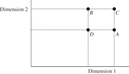
Figure 1.2 Correlation-increasing switch.
If the two dimensions involved in a switch are substitutes, then one counterbalances the deficiency of the other. Since the two dimensions represent similar aspect of well-being because of their closeness in terms of substitutability, the switch makes a poor person poorer and a rich person richer in the concerned dimensions. Consequently, overall welfare position of the society goes down. Similarly, level of welfare should go up under the switch if the dimensions are complements. If the two dimensions are independents, then the welfare function is insensitive to such a switch. A composite index that relies on a dashboard treats the underlying dimensions as independents.
In view of the aforementioned arguments, following Atkinson and Bourguignon (1982) and Bourguignon and Chakravarty (2003), our next axiom can be formally stated as:
- Decreasing Welfare under Correlation Increasing Switch: For all
 ,
,  ,
,  , if
, if  is obtained from X by a correlation-increasing switch, then
  , whenever the dimensions underlying the switch are substitutes.
The axiom clearly indicates under what type of association between dimensions, unambiguous conclusion about direction of welfare change resulting from a correlation-increasing swap can be made. Variants of this axiom when the dimensions are complements and independents can be stated analogously.19,20
Dardanoni (1996) proposed and analyzed a weaker form of the correlation-increasing switch axiom. To get an idea of this, suppose that the achievement matrix  is transformed into a new matrix
  , which clearly indicates the ranks of individuals with respect to their achievements in both the dimensions simultaneously. In fact, we derive
 ![]() from
from ![]() by employing a sequence of correlation-increasing switches so that one person gets top position in all the dimensions, another person gets the second position in all the dimensions, and so on. More precisely, in
by employing a sequence of correlation-increasing switches so that one person gets top position in all the dimensions, another person gets the second position in all the dimensions, and so on. More precisely, in ![]() across all dimensions, the first person is third ranked, the second person is second ranked, and third person is first ranked. Dardanoni (1996) referred to this sequence as unfair rearrangement of dimensional attainments and argued that the transformed social matrix should indicate a lower level of welfare compared to the original one. Analytically,
across all dimensions, the first person is third ranked, the second person is second ranked, and third person is first ranked. Dardanoni (1996) referred to this sequence as unfair rearrangement of dimensional attainments and argued that the transformed social matrix should indicate a lower level of welfare compared to the original one. Analytically,
- Decreasing Welfare under Unfair Rearrangement: For all
 ,
,  ,
,  , if
, if  is obtained from X by a sequence of correlation-increasing switches such that across the dimensions, one individual becomes top ranked, another individual is second ranked, and so on. Then
  .
.
If all the dimensions in an achievement matrix are of the same type, say, substitutes or complements, then the changes in welfare associated with all the switches are unidirectional. But when dimensions are mixed in nature, the directions of change in welfare, as judged by the AELP condition, are as well of mixed type (see footnote 20). Consequently, no unambiguous conclusion about the overall directional change of welfare can be drawn.
1.7 Multidimensional Welfare Functions
A multidimensional social welfare function indicates the level of well-being of a population when achievements of all the individuals in the population, in different dimensions of living, are taken into consideration. Since there may be absence of consensus regarding the choice of a welfare function, the measurement of social welfare is a difficult task. A policy analyst may be forced to present a range of evaluations based on alternative social welfare functions. Each of them is a grand mapping that establishes unambiguous ranking of social alternatives.
In this section, we analyze some of the frequently used multivariate social welfare functions. We begin by reviewing two specific forms of the symmetric utilitarian function  , characterized by Tsui (1995). For the first characterization, in addition to continuity, symmetry, and the strong Pareto principle, Tsui assumed strict quasiconcavity,21 minimal individual separability, introduced by Blackorby et al. (1981), and a strong homotheticity axioms for a general welfare function W defined on M. We state the axioms on the general domain M, and if necessary, a restricted domain will be assumed.
Often from the policy point of view, it becomes necessary to partition a population into two or more subgroups, say, rich and poor subgroups, regional subgroups (see Chapter 2). Then the minimal individual separability axiom enumerates how we can calculate overall welfare in terms of welfare levels of the subgroups. Formally, for all ![]() , for all
, for all ![]() ,
,  , where h is some continuous function,
 ![]() is the submatrix of X that contains the achievements of persons in the nonsingleton subgroup S containing, some, say,
is the submatrix of X that contains the achievements of persons in the nonsingleton subgroup S containing, some, say, ![]() , persons, and
, persons, and ![]() is the complement of
is the complement of ![]() in
in ![]() , that is,
, that is, ![]() includes the achievements of the persons in
includes the achievements of the persons in ![]() .
.
For illustrative purpose, consider the ![]() achievement matrix
achievement matrix  .
.
Suppose that we split the population into two subgroups, say, male and female, whose achievement submatrices are given respectively by  and
and  . Then the separability axiom states that
  .
.
In order to state the next axiom rigorously, we need to consider a positive diagonal matrix: a square matrix whose diagonal elements are positive and off-diagonal elements are zero. A typical ![]() positive diagonal matrix
positive diagonal matrix ![]() can be written as
can be written as ![]() , where
, where ![]() is the
is the ![]() diagonal element and
diagonal element and ![]() .
.
The strong homotheticity postulate requires that for all ![]() , for all
, for all ![]() ,
, ![]() , where
, where ![]() is any
is any ![]() positive diagonal matrix. This condition stipulates that welfare inequality between two social distributions
positive diagonal matrix. This condition stipulates that welfare inequality between two social distributions ![]() and
and ![]() can be equivalently expressed as that between
can be equivalently expressed as that between ![]() and
and ![]() . In other words, the axiom requires invariance of welfare ranking between two distributions under equiproportionate changes in achievements in different dimensions in both the distributions. Note that the proportionality factors need not be the same across dimensions.
. In other words, the axiom requires invariance of welfare ranking between two distributions under equiproportionate changes in achievements in different dimensions in both the distributions. Note that the proportionality factors need not be the same across dimensions.
To clarify the postulate, observe that under the strong Pareto principle, the achievement matrix  becomes welfare superior to
  , that is,
 ![]() . This is because we derive
. This is because we derive ![]() from
from ![]() by decreasing person 1's achievements in dimension 1 by 5 units.
by decreasing person 1's achievements in dimension 1 by 5 units.
For the ![]() diagonal matrix
diagonal matrix  , strong homotheticity demands that
  , which on simplification becomes
  . Thus, when each person's achievement in dimension 1 gets doubled and achievement of each of them in the other dimension remains unchanged, the welfare inequality
 ![]() remains unchanged for the transformed situations as well, that is,
remains unchanged for the transformed situations as well, that is, ![]() holds. Since we can go back to the original inequality
holds. Since we can go back to the original inequality ![]() by postmultiplying each of the two distributions
by postmultiplying each of the two distributions ![]() and
and ![]() in the inequality
in the inequality ![]() by the
by the ![]() diagonal matrix whose first and second diagonal elements are respectively
diagonal matrix whose first and second diagonal elements are respectively ![]() and 1, the converse follows immediately.22
and 1, the converse follows immediately.22
For ![]() ,
, ![]() becomes ordinally equivalent to
becomes ordinally equivalent to  if and only if the six postulates considered earlier hold simultaneously, where
 ![]() is defined as
is defined as

or

![]() for all
for all ![]() , a is a real number and the real numbers b and
, a is a real number and the real numbers b and ![]() ,
, ![]() , are chosen such that U in (1.7) is increasing and strictly concave (see Theorem 1 of Tsui, 1995).
, are chosen such that U in (1.7) is increasing and strictly concave (see Theorem 1 of Tsui, 1995).
The second characterization theorem of Tsui (1995) relies on strong translatability, which requires that for all ![]() , for all
, for all ![]() ,
, ![]() , where A is a
, where A is a ![]() matrix with identical rows such that
matrix with identical rows such that ![]() . This condition claims that welfare inequality between two social matrices can as well be specified in terms of that between the matrices when the achievements of all the persons in a dimension increase/decrease by the same quantity. We refer to the matrix A in the statement of the postulate as a translation matrix.
. This condition claims that welfare inequality between two social matrices can as well be specified in terms of that between the matrices when the achievements of all the persons in a dimension increase/decrease by the same quantity. We refer to the matrix A in the statement of the postulate as a translation matrix.
For the purpose of clarification, let  be a
be a ![]() matrix with identical rows. Thus, each person's achievement in dimension 1 increases by 5 units, and there is a reduction in everybody's achievement in dimension 2 by 4 units. Then given that
matrix with identical rows. Thus, each person's achievement in dimension 1 increases by 5 units, and there is a reduction in everybody's achievement in dimension 2 by 4 units. Then given that ![]() , the axiom requires that
, the axiom requires that ![]() . That is,
. That is,  , which reduces to
  . The axiom also demands that this last inequality should imply the original inequality
 ![]() .
.
Tsui (1995) demonstrated that if in the aforementioned theorem, strong homotheticity is replaced by strong translatability and all other postulates are kept unchanged, then given that ![]() , all the axioms hold simultaneously if and only if
, all the axioms hold simultaneously if and only if ![]() turns out to be ordinally equivalent to
turns out to be ordinally equivalent to  , where
 ![]() is defined as
is defined as

a is an arbitrary real number, the parameters b and ![]() ,
, ![]() , are chosen such that U is increasing and strictly concave (see Theorem 2 of Tsui, 1995). The welfare functions
, are chosen such that U is increasing and strictly concave (see Theorem 2 of Tsui, 1995). The welfare functions  , where the utility functions are of the form (1.7)–(1.9), are symmetric and increasing under a uniform majorization operation.
As we have argued in Section 1.4, a social welfare function can be directly defined on social distributions, represented by achievement matrices. Examples of such welfare standards are the Gajdos–Weymark multidimensional generalized Gini welfare functions (Gajdos and Weymark, 2005). Their characterizations of these welfare functions involve multidimensional twins of the axioms employed by Weymark (1981) to axiomatize the univariate generalized Gini welfare functions.
Of these, homotheticity requires that welfare ranking of two social distributions remains unchanged under common proportional change in dimensional achievements. Formally, for all ![]() ,
, ![]() ,
, ![]() if and only if
if and only if ![]() , where
, where ![]() and
and ![]() is any scalar. To understand this, recall the society's welfare ranking between X13 and X14, which is,
is any scalar. To understand this, recall the society's welfare ranking between X13 and X14, which is, ![]() . Then homotheticity claims that for any
. Then homotheticity claims that for any ![]() , welfare dispreference of
, welfare dispreference of ![]() over
over ![]() is maintained, that is,
is maintained, that is, ![]() should imply
should imply ![]() . The converse should be true as well. Consequently, if
. The converse should be true as well. Consequently, if ![]() , then
, then  should imply
  . The reverse implication can be deduced by multiplying the entries of
 ![]() and
and ![]() by
by ![]() .
.
Two new axioms, strong attribute separability and weak comonotonic additivity, were invoked as well. To state the first of these two axioms, strong attribute separability, for any nonempty ![]() , let
, let ![]() be the submatrix showing achievements of all the individuals with respect to dimensions in S. Then the axiom demands that the conditional social ranking between two submatrices
be the submatrix showing achievements of all the individuals with respect to dimensions in S. Then the axiom demands that the conditional social ranking between two submatrices ![]() and
and ![]() does not depend on the submatrix associated with the dimensions in
does not depend on the submatrix associated with the dimensions in ![]() , where
, where ![]() and
and ![]() are arbitrary.
are arbitrary.
To understand the strong attribute separability postulate, let us derive  from
from ![]() by increasing person 1's achievement in dimension 1 by 10 units. By the strong Pareto principle,
by increasing person 1's achievement in dimension 1 by 10 units. By the strong Pareto principle, ![]() , where
, where ![]() and
and ![]() are respectively the submatrices of
are respectively the submatrices of ![]() and
and ![]() associated with the subset
associated with the subset ![]() of
of ![]() . Note that here
. Note that here ![]() and
and  , which is the same as
 ![]() .
.
Now, consider a third social distribution  so that
  . Then the strong attribute separability axiom demands that the inequality
 ![]() holds if and only if the inequality
holds if and only if the inequality ![]() holds.
holds.
An achievement matrix ![]() is called nonincreasing comonotonic if for any
is called nonincreasing comonotonic if for any ![]() ,
, ![]() , the distribution of achievements in dimension
, the distribution of achievements in dimension ![]() is nonincreasingly ordered, that is,
is nonincreasingly ordered, that is, ![]() . That is, the
. That is, the ![]() person's achievement in any dimension cannot be higher than that of the
person's achievement in any dimension cannot be higher than that of the ![]() person, where
person, where ![]() . We denote the set of all of nonincreasing comonotonic matrices associated with
. We denote the set of all of nonincreasing comonotonic matrices associated with ![]() by
by ![]() . Then weak comonotonic additivity demands that for all
. Then weak comonotonic additivity demands that for all ![]() and
and ![]() for which there exists a
for which there exists a ![]() , such that (i)
, such that (i) ![]() for all
for all ![]() , (ii)
, (ii) ![]() for all
for all ![]() and all
and all ![]() , and (iii)
, and (iii) ![]() ,
, ![]() if and only if
if and only if ![]() .
.
We deduce the matrices ![]() and
and ![]() from
from ![]() and
and ![]() by adding a common distribution of dimension
by adding a common distribution of dimension ![]() to
to ![]() and
and ![]() , respectively. The defining conditions
, respectively. The defining conditions ![]() ,
, ![]() , and
, and ![]() ensure that all the matrices
ensure that all the matrices ![]() and
and ![]() are nonincreasing comonotonic. Further, they all have identical achievement distributions in all the dimensions except k (conditions (i) and (ii)). Then the axiom requires that social ranking between the comonotonic achievement matrices X and Y and that between
are nonincreasing comonotonic. Further, they all have identical achievement distributions in all the dimensions except k (conditions (i) and (ii)). Then the axiom requires that social ranking between the comonotonic achievement matrices X and Y and that between ![]() and
and ![]() coincide.
coincide.
To explain this postulate, note that the matrices ![]() and
and ![]() are nonincreasing comonotonic. In the statement of weak comonotonic additivity, choose
are nonincreasing comonotonic. In the statement of weak comonotonic additivity, choose ![]() and
and  . Consequently,
  and
and  . Evidently,
 ![]() ,
, ![]() , and
, and ![]() are nonincreasing comonotonic, which ensure satisfaction of condition (iii). Conditions (i) and (ii) are verified as well. Then the axiom demands that
are nonincreasing comonotonic, which ensure satisfaction of condition (iii). Conditions (i) and (ii) are verified as well. Then the axiom demands that ![]() implies and is implied by
implies and is implied by ![]() .
.
Assuming that ![]() and
and ![]() , Gajdos and Weymark (2005) demonstrated that a social welfare function
, Gajdos and Weymark (2005) demonstrated that a social welfare function ![]() satisfies continuity, the strong Pareto principle, symmetry, the uniform Pigou–Dalton majorization principle, strong attribute separability, weak comonotonic additivity, and homotheticity if and only if there exist an
satisfies continuity, the strong Pareto principle, symmetry, the uniform Pigou–Dalton majorization principle, strong attribute separability, weak comonotonic additivity, and homotheticity if and only if there exist an ![]() matrix C possessing positive entries
matrix C possessing positive entries ![]() , where
, where ![]() is increasing and
is increasing and  for all
 ![]() ; a (positive) vector
; a (positive) vector ![]() with
with  ; and a scalar
 ![]() such that
such that

if ![]() and
and

if ![]() ;
; ![]() and
and ![]() being arbitrary; and for any
being arbitrary; and for any ![]() ,
, ![]() is the nonincreasingly ordered permutation of
is the nonincreasingly ordered permutation of ![]() , that is,
, that is, ![]() .
.
In (1.10), given any dimension j, ![]() first takes a weighted average of the nonincreasingly ordered dimensional quantities possessed by different persons using increasingly ordered positive weights. Since
first takes a weighted average of the nonincreasingly ordered dimensional quantities possessed by different persons using increasingly ordered positive weights. Since ![]() , these averages are positive for all dimensions
, these averages are positive for all dimensions ![]() . These positive averages are then averaged, using positive weights, over dimensions by raising each of them to the power
. These positive averages are then averaged, using positive weights, over dimensions by raising each of them to the power ![]() , with
, with ![]() being a nonzero real number. Finally,
being a nonzero real number. Finally, ![]() power of the (positive) average obtained at the second stage is taken to arrive at
power of the (positive) average obtained at the second stage is taken to arrive at ![]() . In (1.11), geometric average of the positive numbers
. In (1.11), geometric average of the positive numbers  across dimensions is taken to arrive at the expression for
 ![]() . The two welfare functions (1.10) and (1.11) are linear homogeneous; multiplication of all the achievements across dimensions with a positive scalar will multiply their values by the scalar itself. We refer to these two functions as the Gajdos–Weymark multidimensional generalized Gini homothetic welfare functions, since they apply one-dimensional Gini, more precisely, generalized Gini-type aggregation (see Weymark, 1981).
. The two welfare functions (1.10) and (1.11) are linear homogeneous; multiplication of all the achievements across dimensions with a positive scalar will multiply their values by the scalar itself. We refer to these two functions as the Gajdos–Weymark multidimensional generalized Gini homothetic welfare functions, since they apply one-dimensional Gini, more precisely, generalized Gini-type aggregation (see Weymark, 1981).
Gajdos and Weymark (2005) characterized translatable variants of (1.10) and (1.11). A social welfare function ![]() is called translatable if for all
is called translatable if for all ![]() ,
, ![]() ,
, ![]() if and only if
if and only if ![]() , where
, where ![]() is the
is the ![]() matrix all of whose entries are 1, and c is any real number such that
matrix all of whose entries are 1, and c is any real number such that ![]() . Translatability means that welfare ranking of two social distributions does not change when achievements of all the individuals in all the dimensions are reduced or augmented by the same quantity.
. Translatability means that welfare ranking of two social distributions does not change when achievements of all the individuals in all the dimensions are reduced or augmented by the same quantity.
To illustrate this, consider again the social distribution matrices ![]() and
and ![]() so that
so that ![]() . Suppose that each person's achievements in all the dimensions in matrices
. Suppose that each person's achievements in all the dimensions in matrices ![]() and
and ![]() increase by the same amount 2. Denote the resulting matrices by
increase by the same amount 2. Denote the resulting matrices by ![]() and
and ![]() , respectively. Thus,
, respectively. Thus,  and
and  . Then translatability claims that
 ![]() should imply and is implied by
should imply and is implied by ![]() .
.
If in the characterization of (1.10) and (1.11) we replace homotheticity by translatability and maintain all other axioms, then, given ![]() , Gajdos and Weymark (2005) showed that the only social welfare function
, Gajdos and Weymark (2005) showed that the only social welfare function ![]() for which these axioms hold together are given by
for which these axioms hold together are given by

if the scalar ![]() is nonzero and
is nonzero and

if ![]() , where
, where ![]() is a (positive) vector,
is a (positive) vector, ![]() are the same as in (1.10) and (1.11);
are the same as in (1.10) and (1.11); ![]() and
and ![]() are arbitrary; and for any
are arbitrary; and for any ![]() ,
, ![]() is the nonincreasingly ordered permutation of
is the nonincreasingly ordered permutation of ![]() . While in (1.12) a Kolm–Pollak type aggregation is employed, (1.13) uses a generalized Gini-type aggregation.
. While in (1.12) a Kolm–Pollak type aggregation is employed, (1.13) uses a generalized Gini-type aggregation.
So, if ![]() , first an exponential-type aggregation is employed over individuals and then a logarithmic aggregation is used over the dimensions. Note that if
, first an exponential-type aggregation is employed over individuals and then a logarithmic aggregation is used over the dimensions. Note that if ![]() , we have linear aggregation at each stage. The two standards in (1.12) and (1.13) are translatable. An equal absolute increase in all the dimensional achievements will increase the welfare values in terms of the absolute amount itself. These two standards can be called the Gajdos–Weymark multidimensional generalized Gini translatable welfare functions. It should be clear that strong attribute separability makes the welfare standards (1.10)–(1.13) insensitive to a correlation-increasing switch.
, we have linear aggregation at each stage. The two standards in (1.12) and (1.13) are translatable. An equal absolute increase in all the dimensional achievements will increase the welfare values in terms of the absolute amount itself. These two standards can be called the Gajdos–Weymark multidimensional generalized Gini translatable welfare functions. It should be clear that strong attribute separability makes the welfare standards (1.10)–(1.13) insensitive to a correlation-increasing switch.
Decancq and Lugo (2012) proposed two social welfare functions that involve two-stage aggregations. For the first, a specific procedure following Kolm (1977) is adopted. More precisely, a dashboard of individual dimensional welfare functions is constructed. These dashboard-based welfare metrics are then aggregated to arrive at an overall quantifier of welfare. In the second, which following Kolm (1977), referred to as the individualistic approach, the aforementioned procedure is reversed. In other words, for each individual, a well-being index, defined on the person's dimensional attainments, is designed. These individual metrics are combined to compose a well-being quantifier for the population as a whole (see also Dutta et al., 2003 and Chakravarty and Lugo, 2016).
Formally, for all ![]() and
and ![]() :
:
Here ![]() is the common functional form of welfare statistic of achievements in a dimension, and the argument
is the common functional form of welfare statistic of achievements in a dimension, and the argument ![]() of
of ![]() shows that the index value is calculated for each dimension
shows that the index value is calculated for each dimension ![]() separately. Similarly,
separately. Similarly, ![]() is the common metric of individual well-being. Its value is determined for each of the
is the common metric of individual well-being. Its value is determined for each of the ![]() persons separately.
persons separately.
The following forms of the dimensional and individual indices were considered by Decancq and Lugo (2012):


where ![]() and
and ![]() are arbitrary;
are arbitrary; ![]() is the rank of individual i with respect to his achievement in dimension j;
is the rank of individual i with respect to his achievement in dimension j; ![]() is the weight assigned to his achievement in dimension j,
is the weight assigned to his achievement in dimension j,  , and
, and ![]() is a parameter. The restriction
is a parameter. The restriction ![]() is necessary to seize bottom awareness of aggregator.23 The positive-valued individual well-being standard
is necessary to seize bottom awareness of aggregator.23 The positive-valued individual well-being standard ![]() is continuous, linear homogenous, and strictly concave.
is continuous, linear homogenous, and strictly concave.
The ![]() dimensional dashboard of well-being corresponding to (1.16) is given by
dimensional dashboard of well-being corresponding to (1.16) is given by ![]() . For
. For ![]() ,
, ![]() becomes the Gini welfare function, also known as the Gini mean or the Sen mean, of achievements in dimension
becomes the Gini welfare function, also known as the Gini mean or the Sen mean, of achievements in dimension ![]() . Consequently, in this particular case, the dashboard may be referred to as the Gini welfare dashboard of well-being dimensions.
. Consequently, in this particular case, the dashboard may be referred to as the Gini welfare dashboard of well-being dimensions.
The parameter ![]() in (1.17) has a one-to-one correspondence with the elasticity of substitution between dimensions. In fact, the constant elasticity of substitution (CES) between any two dimensions is given by
in (1.17) has a one-to-one correspondence with the elasticity of substitution between dimensions. In fact, the constant elasticity of substitution (CES) between any two dimensions is given by ![]() . For
. For ![]() , the well-being standard is linear, and substitutability between any two dimensions is perfect. On the other hand, as
, the well-being standard is linear, and substitutability between any two dimensions is perfect. On the other hand, as ![]() , elasticity tends to zero, and there is no possibility for substitution. The scope for substitution decreases as the value of
, elasticity tends to zero, and there is no possibility for substitution. The scope for substitution decreases as the value of ![]() decreases. For
decreases. For ![]() , the constant elasticity is 1. The associated Cobb–Douglas well-being function rules out the possibility of other elasticity values. Flexibility of functional forms of
, the constant elasticity is 1. The associated Cobb–Douglas well-being function rules out the possibility of other elasticity values. Flexibility of functional forms of ![]() cannot be accommodated once
cannot be accommodated once ![]() is assumed. In our future discussion, we will not consider this case. The constancy of the elasticity of substitution between any pair of dimensions is chosen for simplicity. There is no reason for the elasticity of substitution between health and income to be the same as that between income and education. Bourguignon and Chakravarty (2003) argued that the elasticity should depend on dimensional achievements. They also argued that when we have many dimensions, the constancy of the elasticity of substitution between any two dimensions is not realistic. In subsequent discussion here, for simplicity of exposition, we will maintain the constancy assumption.
is assumed. In our future discussion, we will not consider this case. The constancy of the elasticity of substitution between any pair of dimensions is chosen for simplicity. There is no reason for the elasticity of substitution between health and income to be the same as that between income and education. Bourguignon and Chakravarty (2003) argued that the elasticity should depend on dimensional achievements. They also argued that when we have many dimensions, the constancy of the elasticity of substitution between any two dimensions is not realistic. In subsequent discussion here, for simplicity of exposition, we will maintain the constancy assumption.
If the one-dimensional aggregations given by (1.16) and (1.17) are substituted into two initial two-step procedures, the following forms of multidimensional social welfare functions are obtained:


In (1.19), ![]() is the rank of person i on the basis of
is the rank of person i on the basis of ![]() , the vector of nonincreasingly ordered individual well-being levels with
, the vector of nonincreasingly ordered individual well-being levels with  . While, the specific-procedure based on the social welfare function
 ![]() may be regarded as a special case of the Gajdos–Weymark multidimensional generalized Gini social welfare function given by (1.10), the individualistic function
may be regarded as a special case of the Gajdos–Weymark multidimensional generalized Gini social welfare function given by (1.10), the individualistic function ![]() was introduced to the literature by Decancq and Lugo (2012).
was introduced to the literature by Decancq and Lugo (2012).
In ![]() , at the first stage, an individual's well-being measure is determined by considering weighted average of the
, at the first stage, an individual's well-being measure is determined by considering weighted average of the ![]() power of his accomplishments across dimensions and then taking
power of his accomplishments across dimensions and then taking ![]() power of the average itself. At the second stage, a weighted average of these well-being quantities, where the weights are dependent on the distribution of well-being levels across persons, generates the final value of the welfare standard. The function (1.19) is an example of an individualistic index of multidimensional welfare. For
power of the average itself. At the second stage, a weighted average of these well-being quantities, where the weights are dependent on the distribution of well-being levels across persons, generates the final value of the welfare standard. The function (1.19) is an example of an individualistic index of multidimensional welfare. For ![]() , we may refer to it as the Gini individualistic multidimensional welfare function.
, we may refer to it as the Gini individualistic multidimensional welfare function.
The restrictions ![]() and
and ![]() ensure that both
ensure that both ![]() and
and ![]() increase under a uniform majorization transformation. On the other hand, while
increase under a uniform majorization transformation. On the other hand, while ![]() is insensitive to a correlation-increasing switch,
is insensitive to a correlation-increasing switch, ![]() increases under such a switch if the value of
increases under such a switch if the value of ![]() exceeds a lower bound that depends on the weight vector,
exceeds a lower bound that depends on the weight vector, ![]() , and dimensional achievements.
, and dimensional achievements.
Bosmans et al. (2015) considered the double-CES class social welfare function and analyzed its properties. Using a suggestion put forward by Graaff (1977), they considered a decomposition of its associated inequality measure into inequity and efficiency components (see Chapter 2). The welfare function is formally defined as

where ![]() and
and ![]() are arbitrary. Substitution of the explicit form of
are arbitrary. Substitution of the explicit form of ![]() into (1.20) generates the following explicit form of the welfare function (ignoring the cases
into (1.20) generates the following explicit form of the welfare function (ignoring the cases ![]() and
and ![]() ):
):

There is an important difference between the standards ![]() and
and ![]() . While in the former, at the second stage, another constant elasticity-type aggregator is invoked on the individual well-being quantities; in the latter, a rank-dependent weighted average of these quantities is considered.24 The two-parameter family increases under a uniform majorization transformation and decreases under a correlation-increasing switch if and only if
. While in the former, at the second stage, another constant elasticity-type aggregator is invoked on the individual well-being quantities; in the latter, a rank-dependent weighted average of these quantities is considered.24 The two-parameter family increases under a uniform majorization transformation and decreases under a correlation-increasing switch if and only if ![]() . Increasingness under both a correlation-increasing switch and a uniform majorization transformation occurs if and only if
. Increasingness under both a correlation-increasing switch and a uniform majorization transformation occurs if and only if ![]() (Seth, 2013).
(Seth, 2013).
1.8 Concluding Remarks
Our presentation in this chapter relies directly on dimensional achievements of individuals in a society and ignores the role of their preferences. The transfer principles analyzed in the chapter are nonwelfarist conditions since they recommend transfers of resources without involving individual preferences. The conditions of this kind may come into direct conflict with the Pareto principle (see Gibbard, 1979; Fleurbaey and Trannoy, 2003 and Brun and Tungodden, 2004). However, Roemer (1966) turned down the idea that welfarism is bound to occur when the index obeys individual preferences, although he did not “propose a concrete method in order to define a non-welfarist Paretian index” (Fleurbaey, 2006b, p. 233).
Another important unaddressed issue is inclusion of needs in the analysis. In a recent contribution, building on Atkinson and Bourguignon (1987); Moyes (2012) employed the utilitarian rule to develop dominance conditions for comparing household well-beings, where well-being is assumed to depend on income and needs. Consequently, while advocating redistribution of resources across households, needs have to be taken into account (see also Lambert and Ramos, 2002; Ebert, 2004; Shorrocks, 2004). In our context, it will be admirable to investigate the impact of such a notion of transfer under appropriate formulation, say, by considering a necessary variant of the Pigou–Dalton bundle of progressive transfer principle.
References
- Aaberge, R. and A. Brandolini. 2014. Social Evaluation of Multidimensional Count Distributions. ECINEQ Working Paper No. 2014–342.
- Aaberge, R. and A. Brandolini. 2015. Multidimensional Poverty and Inequality. In A.B. Atkinson and F. Bourguignon (eds.), 141–216.
- Aaberge, R. and E. Peluso. 2011. A Counting Approach to Measuring Multidimensional Deprivations. Working Paper No. 07/2011. Universitá Di Verona.
- Adler, M.D. 2012. Well-Being and Fair Distribution: Beyond Cost-Benefit Analysis. Oxford: Oxford University Press.
- Adler, M.D. 2016. Extended Preferences. In M.D. Adler and M. Fleurbaey (eds.), 476–517.
- Adler, M.D. and M. Fleurbaey (eds.) 2016. Oxford Handbook of Well-Being and Public Policy. New York: Oxford University Press.
- Alkire, S. 2016. The Capability Approach and Well-Being Measurement for Public Policy. In M.D. Adler and M. Fleurbaey (eds.), 615–644.
- Alkire, S., J.E. Foster, S. Seth, M.E. Santos, J.M. Roche, and P. Ballón. 2015. Multidimensional Poverty Measurement and Analysis. New York: Oxford University Press.
- Allison, R.A. and J.E. Foster. 2004. Measuring Health Inequality using Qualitative Data. Journal of Health Economics 23: 505–524.
- Anand, S. 1983. Inequality and Poverty in Malaysia: Measurement and Decomposition. New York: Oxford University Press.
- Atkinson, A.B. 1970. On the Measurement of Inequality. Journal of Economic Theory 2: 244–263.
- Atkinson, A.B. 2003. Multidimensional Deprivation: Contrasting Social Welfare and Counting Approaches. Journal of Economic Inequality 1: 51–65.
- Atkinson, A.B. and F. Bourguignon. 1982. The Comparison of Multidimensioned Distributions of Economic Status. Review of Economic Studies 49: 183–201.
- Atkinson, A.B. and F. Bourguignon. 1987. Income Distributions and Differences in Needs. In G. Feiwel (ed.) Arrow and the Foundations of the Theory of Economic Policy. New York: MacMillan, 350–370.
- Atkinson, A.B. and F. Bourguignon (eds.). 2015. Handbook of Income Distribution, Vol. 2A. Amsterdam: North Holland.
- Atkinson, A.B., B. Cantillon, E. Marlier, and B. Nolan. 2002. Social Indicators: The EU and Social Exclusion. Oxford: Oxford University Press.
- Balckorby, C., W. Bossert, and D. Donaldson. 2005. Population Issues in Social Choice Theory, Welfare Economics and Ethics. New York: Cambridge University Press.
- Banerjee, A.K. 2014. A Multidimensional Lorenz Domination Relation. Social Choice and Welfare 42: 171–191.
- Banerjee, A.V. and E. Duflo. 2011. Poor Economics: A Radical Rethinking of the Way to Fight Global Poverty. New York: Public Affairs.
- Barbera, S., P.J. Hammond, and C. Seidl. (eds.). 2004. Handbook of Utility Theory, Vol. 2: Extensions. Boston: Kluwer Academic.
- Basu, K. 1980. Revealed Preference of Government. Cambridge: Cambridge University Press.
- Basu, K. and L.F. López-Calva. 2011. Functionings and Capabilities. In K.J. Arrow, A.K. Sen, and K. Suzumura (eds.) Handbook of Social Choice and Welfare, Vol. II. Amsterdam: North Holland, 153–187.
- Becker, G.S., T.J. Philipson, and R.R. Soares. 2005. The Quantity and Quality of Life and the Evolution of World Inequality. American Economic Review 95: 277–291.
- Blackorby, C. and D. Donaldson. 1982 Ratio-scale and Translation-scale Full Interpersonal Comparisons without Domain Restrictions: Admissible Social-evaluation Functions. International Economic Review 23: 249–268.
- Blackorby, C, D. Donaldson, and M. Auersperg. 1981. A New Procedure for the Measurement of Inequality within and among Population Subgroups. Canadian Journal of Economics 14: 665–685.
- Blackorby, C., D. Donaldson, and J.A. Weymark: 1984. Social Choice Theory with Interpersonal Utility Comparisons: A Diagrammatic Introduction. International Economic Review 25: 2–31.
- Boadway, R. 2016. Cost-Benefit Analysis. In M.D. Adler and M. Fleurbaey (eds.), 47–81.
- Boelhouwer, J. 2002. Quality of Life and Living Conditions in the Netherlands. Social Indicators Research 60: 89–113.
- Bosmans, K., K. Decancq, and E. Ooghe. 2015. What do Normative Indices of Multidimensional Inequality Really Measure? Journal of Public Economics 130: 94–104.
- Bosmans, K., L. Lauwers, and E. Ooghe. 2009. A Consistent Multidimensional Pigou–Dalton Transfer Principle. Journal of Economic Theory 144: 1358–1371.
- Bossert, W., S.R. Chakravarty, and C. D'Ambrosio. 2013. Multidimensional Poverty and Material Deprivation with Discrete Data. Review of Income and Wealth 59: 29–43.
- Bossert, W. and J.A. Weymark. 2004. Utility in Social Choice. In S. Barbera, P. Hammond, and C. Seidl (eds.), 1099–1177.
- Bourguignon, F. 1999. Comment on Multidimensioned Approaches to Welfare Analysis by E. Maasoumi. In J. Silber (ed.) Handbook of Income Inequality Measurement. London: Kluwer Academic, 477–484.
- Bourguignon, F. and S.R. Chakravarty. 2003. The Measurement of Multidimensional Poverty. Journal of Economic Inequality 1: 25–49.
- Brandolini, A. 2009. On Synthetic Indices of Multidimensional Well-being: Health and Income Inequalities in France, Germany, Italy and the United Kingdom. In R. Gotoh, P. Dumouchel (eds.) Against Injustice: The New Economics of Amartya Sen. Cambridge: Cambridge University Press, 221–251.
- Brandolini, A. and D'Alessio. 1998. Measuring Well-Being in the Functioning Space. Bank of Italy: Rome.
- Broome, J. 2016. The Well-Being of Future Generations. In M.D. Adler and M. Fleurbaey (eds.), 901–927.
- Brun, B.C. and B. Tungodden. 2004. Non-welfaristic Theories of Justice: Is “the Intersection Approach” a Solution to the Indexing Impasse? Social Choice and Welfare 22: 49–60.
- Card, D. 1999. The causal Effect of Education on Earnings. In O. Ashenfelter and D. Card (eds.) Handbook of Labor Economics. Vol. III. Amsterdam: North Holland, 1801–1863.
- Cerioli, A. and Zani, S. 1990. A Fuzzy Approach to the Measurement of Poverty. In C. Dagum and M. Zenga (eds.) Income and Wealth Distribution, Inequality and Poverty. New York: Springer, 272–284.
- Chakravarty, S.R. 2009. Inequality, Polarization and Poverty: Advances in Distributional Analysis. New York: Springer.
- Chakravarty, S.R. 2010. Metodología de la Medición Multidimensional de la Pobreza Para México. In N.M. Martini (ed.) Medición Multidimensional de la Poberza en México. Coneval: el Colegio de México, 281–322.
- Chakravarty, S.R. and C. D'Ambrosio. 2006. The Measurement of Social Exclusion. Review of Income and Wealth 52: 377–398.
- Chakravarty, S.R. and M.A. Lugo. 2016. Multidimensional Indicators of Inequality and Poverty. In M.D. Adler and M. Fleurbaey (eds.), 246–285.
- Chakravarty, S.R. and C. Zoli. 2012. Stochastic Dominance Relations for Integer Variables. Journal of Economic Theory 147: 1331–1341.
- Châteauneuf, A. and P. Moyes. 2006. A Non-welfarist Approach to Inequality Measurement. In M. McGillivray (ed.) Inequality, Poverty and Well-being. London: Palgrave Macmillan, 22–65.
- Cheli, B. and A. Lemmi. 1995. A “Totally” Fuzzy and Relative Approach to the Multidimensional Analysis of Poverty. Economic Notes 24: 115–133.
- Cherchye, L., W. Moesen, N. Rogge and T. van Puyenbroeck. 2007a. An Introduction to ‘Benefit of the Doubt’ Composite Indicators. Social Indicators Research 82: 111–145.
- Cherchye, L., W. Moesen, N. Rogge, T. van Puyenbroeck , M. Saisana, A. Saltelli, R. Liska, and S. Tarantola. 2007b. Creating Composite Indicators with DEA and Robustness Analysis: The Case of Technology Achievement Index. Journal of the Operations Research Society 59: 231–251.
- Cherchye, L., E. Ooghe, and T. van Puyenbroeck. 2008. Robust Human Development Ranking. Journal of Economic Inequality 6: 287–321.
- Chipman, J.S. 1977. An Empirical Implication of Auspitz-Edgeworth-Lieben-Pareto Complementarity. Journal of Economic Theory 14: 228–231.
- Chowdhury, S. and L. Squire. 2006. Setting Weights to Aggregate Indices: An Application to the Commitment to Development Index and Human Development Index. Journal of Development Studies 42: 761–771.
- Clark, A.E. 2016. SWB as a Measure of Individual Well-Being. In M.D. Adler and M. Fleurbaey (eds.), 518–552.
- Cummins, R.A. 1996. Domains of Life Satisfaction: An Attempt to Order Chaos. Social Indicators Research 38: 303–328.
- d'Aspremont, C. and L. Gevers. 1977. Equity and Informational Basis of Collective Choice. Review of Economic Studies 44: 199–209.
- d'Aspremont, C. and L. Gevers. 2002. Social Welfare Functionals and Interpersonal Comparability. In K.J. Arrow, A.K. Sen, and K. Suzumura (eds.) Handbook of Social Choice and Welfare, Vol. 1. Amsterdam: North-Holland, 459–541.
- Dalton, H. 1920. The Inequality of Incomes. London: Routledge.
- Dardanoni, V. 1996. On Multidimensional Inequality Measurement. Research on Economic Inequality 6: 201–205.
- Dasgupta, P., A.K. Sen, and D. Starrett. 1973. Notes on the Measurement of Inequality. Journal of Economic Theory 6: 180–187.
- de Kruijk, H. and M. Rutten. 2007. Weighting Dimensions of Poverty based on People's Priorities: Constructing a Composite Poverty Index for the Maldives. Centre for International Studies. University of Toronto.
- Deaton, A. 1992. Understanding Consumption. New York: Oxford University Press.
- Deaton, A. 1997. The Analysis of Household Surveys: A Microeconometric Approach to Development Policy. Baltimore, MD: Johns Hopkins University Press.
- Deaton, A. and M. Grosh. 2000. Consumption. In M. Grosh and P. Glewwe (eds.) Designing Household Survey Questionnaire for Developing Countries: Lessons from 15 Years of Living Standard Measurement Study. Washington, DC: World Bank, 91–133.
- Decancq, K. 2012. Elementary Multivariate Rearrangements and Stochastic Dominance on a Frechét Class. Journal of Economic Theory 147: 1450–1459.
- Decancq, K. 2013. Copula-based Measurement of Dependence between Dimensions of Well-being. Oxford Economic Papers 66: 681–701.
- Decancq, K., M. Fleurbaey, and E. Schokkaert (2015). Inequality, Income and Well-Being. In A.B. Atkinson and F. Bourguignon (eds.), 67–140.
- Decancq, K. and M.A. Lugo. 2012. Inequality of Well-Being: A Multidimensional Approach. Economica 79: 721–746.
- Decancq, K. and D. Neumann. 2016. Does the Choice of Well-Being Measure Matter Empirically? In M.D. Adler and M. Fleurbaey (eds.), 553–587.
- Decancq, K. and E. Ooghe. 2010. Has the World Moved Forward? A Robust Multidimensional. Evaluation. Economics Letters 107: 266–269. 81–701.
- Decancq, K. and E. Schokkaert. 2016. Beyond GDP: Using Equivalent Incomes to Measure Well-being in Europe. Social Indicators Research 126: 21–55.
- Desai, M. and A. Shah. 1988. An Econometric Approach to the Measurement Poverty. Oxford Economic Papers 40: 505–522.
- Despotis, D.K. 2005a. Measuring Human Development via Data Envelopment Analysis: The Case of Asia and the Pacific. Omega 33: 385–390.
- Despotis, D.K. 2005b. A Reassessment of the Human Development via Data Envelopment Analysis. Journal of the Operational Research Society 56: 969–980.
- Deutsch, J. and J. Silber. 2005. Measuring Multidimensional Poverty: An Empirical Comparison of Various Approaches. Review of Income and Wealth 51: 145–174.
- Di Tommaso, M.L. 2006. Measuring the Well-being of Children using a Capability Approach An Application to Indian Data. Working Paper 05-06, Centre for Household, Income, Labour and Demographic Economics.
- Diez, H., M.C. Lasso de la Vega, A. de Sarachu, and A. Urrutia. 2007. A Consistent Multidimensional Generalization of the Pigou-Dalton Transfer Principle: An Analysis. B.E. Journal of Theoretical Economics 7. Available at: http:/www.bepress.com/bejte/vol7/iss1/art45.
- Donaldson D. and J.A. Weymark. 1980. A Single Parameter Generalization of the Gini indices of inequality. Journal of Economic Theory 22: 67–86.
- Doyal, L. and I. Gough. 1991. A Theory of Human Need. Basinkstoke: Macmillan.
- Duclos, J.-Y. and L. Tiberti. 2016. Multidimensional Poverty Indices: A Critical Assessment. In M.D. Adler and M. Fleurbaey (eds.), 677–710.
- Dutta, I. , P.K. Pattanaik, and Y. Xu. 2003. On Measuring Deprivation and the Standard of Living in a Multidimensional Framework on the Basis of Aggregate Data. Economica 70: 197–221.
- Easterlin, R. 2000. The Worldwide Standard of Living since 1800. Journal of Economic Perspectives 14: 7–26.
- Ebert, U. 1988. Measurement of Inequality: An Attempt at Unification and Generalization. Social Choice and Welfare 5: 147–169.
- Ebert, U. 2004. Social Welfare, Inequality and Poverty when Needs Differ. Social Choice and Welfare 23: 415–448.
- Elson, D., S. Fukuda-Parr, and P. Vizard (eds.) 2011. Journal of Human Development and Capabilities 12: Special Issue on Human Rights and Capabilities.
- Epstein, L.G. and S.M. Tanny. 1980. Increasing Generalized Correlation: A Dentition and Some Economic Consequences. Canadian Journal of Economics 13: 16–34.
- Farina, F. and E. Savaglio (eds.) 2006. Inequality and Economic Integration. London: Routledge.
- Ferrer-i Carbonell, A. and P. Frijters. 2004. How Important is Methodology for the Estimates of the Determinants of Happiness? Economic Journal 114: 641–659.
- Fleurbaey, F. 2006a. Capabilities, Functionings and Refined Functionings. Journal of Human Development 7: 299–310.
- Fleurbaey, F. 2006b. Social Welfare, Priority to the Worst-off and the Dimensions of Individual Well-being. In F. Farina and E. Savaglio (eds.), 222–263.
- Fleurbaey, F. 2009. Beyond the GDP: The Quest for a Measure of Social Welfare. Journal of Economic Literature 47: 1029–1075.
- Fleurbaey, F. and D. Blanchet. 2013. Beyond GDP: Measuring Welfare and Assessing Sustainability. Oxford: Oxford University Press.
- Fleurbaey, F. and G. Gaulier. 2009. International Comparisons of Living Standards by Equivalent Incomes. Scandinavian Journal of Economics 111: 597–624.
- Fleurbaey, M. and P.J. Hammond. 2004. Interpersonally Comparable Utility. In S. Barbera, P.J. Hammond, and C. Seidl (eds.), 1179–1285.
- Fleurbaey, F. and F. Maniquet. 2011. A Theory of Fairness and Social Welfare. New York: Cambridge University Press.
- Fleurbaey M. and Ph. Michel. 2001. Transfer Principles and Inequality Aversion, with an Application to Optimal Growth. Mathematical Social Sciences 42: 1–11.
- Fleurbaey, F., E. Schokkaert, and K. Decancq. 2015. Happiness, Equivalent Income and Respect for Individual Preferences. Economica 82: 1082–1106.
- Fleurbaey M. and A. Trannoy. 2003. The Impossibility of a Paretian Egalitarian. Social Choice Welfare 21: 319–329.
- Foster, J.E., M. McGillivray, and S. Seth. 2013a. Composite Indices: Rank Robustness, Statistical Association and Redundancy. Econometric Reviews 22: 35–56.
- Foster, J.E. and A.K. Sen. 1997. On Economic Inequality: After a Quarter Century, Annex to Enlarged Edition of On Economic Inequality by A.K. Sen. Oxford: Clarendon Press.
- Foster, J.A., S. Seth, M. Lokshin, and Z. Sajaia. 2013b. A Unified Approach to Measuring Poverty and Inequality: Theory and Practice. Washington, DC: World Bank.
- Gajdos, T. and J.A. Weymark. 2005. Multidimensional Generalized Gini Indices. Economic Theory 26: 471–496.
- Gibbard, A. 1979. Disparate Goods and Rawls' s Difference Principle: A Social Choice Theoretic Treatment. Theory and Decision 11: 267–288.
- Graaff, J. de V. 1977. Equity and Efficiency as Components of the General Welfare. South African Journal of Economics 45: 362–375.
- Graham, C. 2016. Subjective Well-Being in Economics. In M.D. Adler and M. Fleurbaey (eds.), 424–450.
- Grusky, D.B. and R. Kanbur.(eds.) 2006. Poverty and Inequality. Stanford University Press: Stanford, CA.
- Halleröd, B. 1995. The Truly Poor: Direct and Indirect Consensual Measurement of Poverty in Sweden. Journal of European Social Policy 5: 111–129.
- Halleröd, B. 1996. Deprivation and Poverty: A Comparative Analysis of Sweden and Great Britain. Acta Sociologica 39: 141–168.
- Hammond, P.J. 1976. Why Ethical Measures of Inequality Need Interpersonal Comparisons? Theory and Decision 7: 263–274.
- Hammond, P.J. 1991. Interpersonal Comparisons of Utility : Why they are and how they should be made ? In J. Elster and J.E. Roemer (eds.) Interpersonal Comparisons of Well-Being. Cambridge: Cambridge University Press, 200–254.
- Haughton, J.H. and S.R. Khandker. 2009. Handbook on Poverty and Inequality. Washington, DC: World Bank.
- Hentschel, J. and P. Lanjouw. 2000. Household Welfare Measurement and the Pricing of Basic Services. Journal of International Development 12: 13–27.
- Hicks, D. 1997. The Inequality-Adjusted Human Development Index: A constructive Proposal. World Development 25: 1283–1298.
- Hicks, N. and P. Streeten. 1979. Indicators of Development: The Search for a Basic Needs Yardstick. World Development 7: 567–580.
- Hobijn, B. and P.H. Franses. 2001. Are Living Standards Converging? Structural Change and Economic Dynamics 12: 171–200.
- Høyland, B., K. Moene, and F. Willumsen. 2012. The Tranny of International Index Ranking. Journal of Development Economics 97: 1–14.
- Jayraj, D. and S. Subramanian. 2009. A Chakravarty-D'Ambrosio Approach View of Multidimensional Deprivation: Some Estimates for India. Economic and Political Weekly 45: 53–65.
- Jenkins, S. and J. Micklewright.(eds.) 2007. Inequality and Poverty Reexamined. Oxford: Oxford University Press.
- Jorgenson, D.W. and D.T. Slesnick. 1984. Aggregate Consumer Behavior and the Measurement of Inequality. Review of Economic Studies 51: 369–392.
- Kannai, Y. 1980. The ALEP Definition of Complementarity and Least Concave Utility Functions. Journal of Economic Theory 22: 115–117.
- Klasen, S. 2000. Measuring Poverty and Deprivation in South Africa. Review of Income and Wealth 46: 33–58.
- Klugman, J. 2002. A Sourcebook of Poverty Reduction Strategies. Washington, DC: World Bank.
- Kolm, S.C. 1976. Unequal inequalities I. Journal of Economic Theory 12: 416–442.
- Kolm, S.C. 1977. Multidimensional Egalitarianism. Quarterly Journal of Economics 91: 1–13.
- Krishnakumar, J. 2007. Going Beyond Functionings to Capabilities: An Econometric Model to Explain and Estimate Capabilities. Journal of Human Development 7: 39–63.
- Krishnakumar, J. and P. Ballon. 2008. Estimating Basic Capabilities: A Structural Equation Model Approach Applied to Bolivian Data. World Development 36: 992–1010.
- Krishnakumar, J. and A. Nadar. 2008. On Exact Statistical Properties of Multidimensional Indices based on Principal Components, Factor Analysis, MIMIC and Structural Equation Models. Social Indicators Research 86: 481–496.
- Kuklys, W. 2005. Amartya Sen's Capability Approach: Theoretical Insights and Empirical Applications. Berlin: Springer.
- Lambert, P.J. and X. Ramos. 2002. Welfare Comparisons: Sequential Procedures for Heterogeneous Populations. Economica 69: 549–562.
- Lasso de la Vega, M.C. 2010. Counting Poverty Orderings and Deprivation Curves. Research on Economic Inequality 18: 153–172.
- Lasso de la Vega, M.C. and A. Urrutia. 2011. Characterizing How to Aggregate Individuals Deprivations in a Multidimensional Framework. Journal of Economic Inequality 9: 183–194.
- Lasso de la Vega, M.C., A. Urrutia, and A. Sarachu. 2009. The Bourguignon and Chakravarty Multidimensional Poverty Family: A Characterization. ECINEQ WP 2009–109.
- Lasso de la Vega, M.C., A. Urrutia, and A. Sarachu. 2010. Characterizations of Multidimensional Inequality Measures which fulfil the Pigou-Dalton Bundle Principle. Social Choice and Welfare 35: 319–329.
- Lewbel, A. and K. Pendakur. 2008. Equivalence Scales. In S. Durlauf and L.E. Blume (eds.) The New Palgrave Dictionary of Economics, Vol. 3, Second Edition. Basingstoke: Palgrave Macmillan, 26–29.
- Mack, J., S. Lansley. 1985. Poor Britain. London: Allen and Unwin.
- Mahlberg, B. and M. Obersteiner. 2001. Remeasuring the HDI by Data Envelopment Analysis. Interim Report IR-01-069. International Institute for Applied System Analysis.
- Marshall, A.W., I. Olkin, and B.C. Arnold. 2011. Inequalities: Theory of Majorization and Its Applications. New York: Springer.
- Mascherini, M. and B. Hoskins. 2008. Retrieving the Expert Opinion on Weights for the Active Citizenship Composite Indicator. European Commission.
- Mayer, S.E. and C. Jencks. 1989. Poverty and Distribution of Material Hardship. Journal of Human Resources 24: 88–114.
- Moldan, B. and S. Billharz. 1997. Indicators of Sustainable Development. Chichester: John Wiley.
- Moyes, P. 2012. Comparisons of Heterogeneous Distributions and Dominance Criteria. Journal of Economic Theory 147: 1351–1383.
- Murphy, K.M. and R.H. Topel. 2006. The value of Health and Longevity. Journal of Political Economy 114: 871–904.
- Narayan, D. 2000. Voices of the Poor: Can Anyone Hear Us? Washington, DC: World Bank.
- Nardo, M. , M. Saisana, A. Saltelli, S. Tarantola, A. Hoffman, and E. Giovannini. 2005. Handbook on Constructing Composite Indicators: Methodology and User Guide. OECD Publishing.
- Neumayer, E. 2003. Beyond Income: Convergence in Living Standards, Big Time. Structural Change and Economic Dynamics 14: 275–296.
- Noble, M, G. Wright, G. Smith, and C. Dibben. 2006. Measuring Multiple Deprivation at the Small Area Level. Environment and Planning 38: 169–185.
- Noorbakhsh, F. 1998. The Human Development Index: Some Technical Issues and Alternative Indices. Journal of International Development 10: 589–605.
- Nussbaum, M.C. 2000. Women and Human Development: The Capabilities Approach. Cambridge: Cambridge University Press.
- Osberg, L. and A. Sharpe. 2002. An Index of Economic Well-being for Selected Countries. Review of Income and Wealth 48: 291–316.
- Permanyer, I. 2011. Assessing the Robustness of Composite Indices Rankings. Review of Income and Wealth 57: 306–326.
- Permanyer, I. 2012. Uncertainty and Robustness in Composite Indices Rankings. Oxford Economic Papers 64: 57–79.
- Pogge, T. 2002. Can the Capability Approach be justified? Philosophical Topics 30: 167–228
- Pollak, R.A. 1971. Additive Utility Functions and Linear Engel Curves. Review of Economic Studies 38: 401–413.
- Qizilbash, M., S. Fukuda-Parr, and S. Subramanian (eds.) 2006. Journal of Human Development 7, Number 3: Special Issue: Selected Papers from the 5th International Conference on the Capability Approach and 2005 International Conference of the Human Development and Capability Association.
- Ramsay, M. 1992. Human Needs and the Market, Aldershot: Avebury
- Ravallion, M. 1994. Poverty Comparisons. Chur, Switzerland: Harwood.
- Ravallion, M. 1996. Issues in Measuring and Modelling Poverty. Economic Journal 106: 1328–1343.
- Ravallion, M. 1997. Good and Bad Growths: The Human Development Reports. World Development 25: 631–638.
- Ravallion, M. 2008. Poverty Lines. In S.N. Durlauf and L.E. Blume (eds.) The New Palgrave Dictionary of Economics, Vol. 3, Second Edition. Basingstoke: Palgrave Macmillan.
- Ravallion, M. 2011. On Multidimensional Indices of Poverty. Journal of Economic Inequality 9: 235–248.
- Ravallion, M. 2012. Troubling Tradeoffs in the Human Development Index. Journal of Development Economics 99: 201–209.
- Rawls, J. 1971. A Theory of Justice. Cambridge: Harvard University Press.
- Roberts, K.W.S. 1980. Interpersonal Comparability and Social Choice Theory. Review of Economic Studies 47: 421–439.
- Robeyns, I. 2009. Justice as Fairness and the Capability Approach. In K. Basu and R. Kanbur (eds.) Arguments for a Better World: Essays in Honor of Amartya Sen. New York: Oxford University Press, 397–413.
- Roemer, J.E. 1966. Theories of Distributive Justice. Cambridge, MA: Harvard University Press.
- Saaty, R.W. 1987. The Analytic Hierarchy Process: What it is and How it is used. Mathematical Modelling 9: 161–176.
- Saisana, M., A. Saltelli and S. Tarantola. 2005. Uncertainty and Sensitivity Analysis as Tools for the Quality Assessment of Composite Indicators. Journal of the Royal Statistical Society: Series A 168: 307–323.
- Savaglio, E. 2006a. Three Approaches to the Analysis of Multidimensional Inequality. In F. Farina and E. Savaglio (eds.), 264–277.
- Savaglio, E. 2006b. Multidimensional Inequality with Variable Population Size. Economic Theory 28: 85–94.
- Schokkaert, E. 2007. Capabilities and Satisfaction with Life. Journal of Human development 8: 415–430.
- Schokkaert, E., L. Van Ootegem, and E. Verhofstadt. 2009. Measuring job Quality and Job Satisfaction. FEB Working Article 2009/620.
- Sen, A.K. 1973. On Economic Inequality. New York: Norton.
- Sen, A.K. 1974. Informational Bases of Alternative Welfare Approaches: Aggregation and Income Distribution. Journal of Public Economics 3: 387–403.
- Sen, A.K. 1977. On Weights and Measures: Informational Constraints in Social Welfare Analysis. Econometrica 45: 1539–1572.
- Sen, A.K. 1985. Commodities and Capabilities. Amsterdam: North-Holland.
- Sen, A.K. 1992. Inequality Re-examined. Cambridge, MA: Harvard University Press.
- Sen, A.K. 2009. The Idea of Justice. Cambridge, MA: Harvard University Press.
- Sen, A.K. and M.C. Nussbaum(eds.). 1993. The Quality of Life. Oxford: Clarendon Press.
- Seth, S. 2013. A Class of Distribution and Association Sensitive multidimensional Welfare Indices. Journal of Economic Inequality 11: 133–162.
- Shorrocks, A.F. 2004. Inquality and Welfare Evaluation of Heterogenous Income Distribution. Journal of Economic Inequality 2: 193–218.
- Slottje, D., G. Scully, J.G. Hirschberg, and K. Hayes. 1991. Measuring the Quality of Life across Countries. Berkeley, CA: Westview Press.
- Somarriba, N. and B. Pena. 2009. Synthetic Indicators of Quality of Life in Europe. Social Indicators Research 94: 115–133.
- Srinivasan, T.N. 1994. Human Development: A New Paradigm or Reinvention of the Wheel? American Economic Review Papers and Proceedings 84: 238–243.
- Stevens, S.S. 1946. On the Theory of Scales of Measurement. Science NS 103: 677–680.
- Stewart, F. 1985. Basic Needs in Developing Countries. Baltimore, MD: Johns Hopkins University Press.
- Stiglitz, J.E., A. Sen, and J.-P. Fitoussi. 2009. Report by the Commission on the Measurement of Economic Performance and Social Progress, www.stiglitz-sen-fitoussi.fr.
- Streeten, P. 1981. First Things First: Meeting Basic Human Needs in Developing Countries. New York: Oxford University Press.
- Tchen, A. 1980. Inequalities for Distributions with Given Margins. The Annals of Probability 8: 814–827.
- Thorbecke, E. 2008. Multidimensional Poverty: Conceptual and Measurement Issues. In N. Kakwani and J. Silber (eds.) The Many Dimensions of Poverty. New York: Palgrave, 3–19.
- Townsend, P. 1979. Poverty in the United Kingdom: A Survey of Household Resources and Standards of Living. London: Peregrine Books.
- Trannoy, A. 2006. Multidimensional Egalitarianism and the Dominance Approach: A Lost Paradise? In F. Farina and E. Savaglio (eds.), 284–302.
- Tsui, K.-Y. 1995. Multidimensional Generalizations of the Relative and Absolute Indices: The Atkinson-Kolm-Sen Approach. Journal of Economic Theory 67: 251–265.
- Tsui, K.-Y. and J.A. Weymark. 1997. Social Welfare Orderings for Ratio-scale Measurable Utilities. Economic Theory 10: 241–256.
- United Nations Development Program. 2005. Human Development Report 2005. New York: Oxford University Press.
- Weymark, J.A. 1981. Generalized Gini Inequality Indices. Mathematical Social Sciences 1: 409–430.
- Weymark, J.A. 2006. The Normative Approach to the Measurement of Multidimensional Inequality. In F. Farina and E. Savaglio (eds.), 303–328.
- Weymark, J.A. 2016. Social Welfare Functions. In M.D. Adler and M. Fleurbaey (eds.), 126–159.
- Wolff, H., H. Chong, and M. Auffhammer. 2011. Classification, Detection and Consequences of Data Error: Evidence from the Human Development Index. Economic Journal 121: 843–870.
- Wolff, J. and De-Shalit, A. 2007. Disadvantage. New York: Oxford University Press.
- World Bank. 2000. World Development Report 2000/2001. Washington, DC: World Bank.
- World Bank. 2006. World Development Report 2006: Equity and Development. Washington, DC: World Bank.
- Zaim, O., R. Fare, and S. Grosskopf. 2001. An Economic Approach to Achievement and Improvement Indexes. Social Indicators Research 56: 91–118.
- Zhou, P., B.W. Ang, and D.Q. Zhou. 2010. Weighting and Aggregation in Composite Indicator Construction: A Multiplicative Optimization Approach. Social Indicators Research 96: 169–181.