
Chapter 3
A Synthesis of Multidimensional Poverty
3.1 Introduction
Poverty remains a burning problem in many countries of the world even in the early twenty-first century. Many people in such countries and in many relatively rich countries as well need to struggle in making ends meet. Consequently, removal of poverty continues to be one of the major economic policies for many people in the world.
We have argued explicitly in earlier chapters that well-being of a population is a multidimensional phenomenon (see Stiglitz et al., 2009). Hence, poverty can be regarded as a manifestation of insufficiency of achievements in different dimensions of well-being. The emphasis on multidimensionality of poverty arises from the cognizance that income by itself cannot capture many important factors that may downgrade a person to poverty. Reckless spending by a very wealthy person on consumption of unhealthy food items is likely to deteriorate health status. In other words, this income-rich person becomes deprived in health dimension of well-being. A wealthy person cannot increase the quantity of an inadequately supplied public good by spending money on his own.
In a study for Montevideo, the capital of Uruguay, Katzman (1989) noted that 13% of households were poor in the income dimension but did not encounter deprivation with respect to basic needs and the opposite happened for 7.5% of the households. Ruggeri Laderchi (1997) employed Chilean data to conclude that income alone is unable to furnish an all-inclusive picture of poverty. In their study, Stewart et al. (2007) noted that 53% of undernourished Indian children did not belong to income-poor households. It was noted as well that 53% of the children coming from the households that were poverty stricken in the income dimension were not undernourished. These studies clearly indicate income in itself does not convey deprivations in nonmonetary dimensions (see also Bradshaw and Finch, 2003 and Alkire et al., 2015).
Attempts to cluster dimensional achievements, using prices as respective weights, into a composite figure indicating overall achievement performance may not be unambiguously acceptable. The reason behind this is that there may not exist a suitable price system that enables us to aggregate individual achievements into a single number, which can be compared with an income poverty line to judge whether the person is poor or not. This is the well-known income method adopted in many earlier studies. This may be due to nonexistence of markets for some dimensions. Examples include public goods, consumption and production externalities, and informational asymmetry. This is true as well for rationed goods (see Tsui, 2002 and Bourguignon and Chakravarty, 2003).
A very important reason for assessing poverty from multidimensional perspective is based on a concrete recommendation made by the European Union. In March 2000, in the Lisbon European Union Council, it was decided to shift poverty measurement policy from income dimension to a multidimensional framework. Five objectives on employment, innovation, education, social exclusion, and climate/energy, to be achieved by 2020, were laid by the European Union.
Among different methods, suggested for the measurement of multidimensional poverty, are the basic needs, social exclusion, and capability approaches. The basic needs formulation to multidimensional poverty is concerned with the definitions of minimum resources required to maintain barely “physical efficiency” (Townsend, 1954, p. 131; see also Streeten et al., 1981). At the individual level, social exclusion can be regarded as a person's exclusion from participation in primary economic and social activities of human well-being (see, among others, Akerlof, 1997; Atkinson, 1998; Atkinson et al., 2002, 2017). According to Sen (1993), the capability approach relies on an outlook of living as a mixture of different “doings” and “things”. Quality of life needs to be evaluated with respect to attainment of valuable functiongs. (See also Sen, 1987). In this method, functionings and capability are two integral aspects of poverty measurement. Capability deprivation incorporates the true concept of poverty experienced by people in everyday life (Sen, 1999, p. 87). The deprived individuals are declined access to many primary social and political rights. Poverty can be conceived as an overall construct involving different aspects of living conditions.
In the direct method, each person possesses a vector of quantities of needs that serve as different dimensions of human well-being and a direct procedure of pinpointing the poor substantiates whether the person has “minimally acceptable levels” (Sen, 1992, p. 139) of achievements in these dimensions. These “minimally acceptable” quantities appear as the threshold limits or cutoff points for different dimensions. These demarcation lines are assumed to be exogenously given; they do not depend on the distributions of achievements in different dimensions. They are determined independently of the achievement distributions. A person whose achievements in different dimensions do not fall below the corresponding threshold limits is treated as nonpoor. On the other hand, if a person's achievement in a dimension is lower than the associated threshold limit, then he is counted as deprived in the dimension. Given a well-defined rule of diagnosing the set of poor persons, the construction of a poverty index involves aggregation of shortfalls of dimensional achievements from respective thresholds, in other words, of the dimensionwise deprivations. More generally, in the direct method, joint distributions of disadvantages and interconnections between disadvantages are taken into account.
It will now be worthwhile to make a systematic comparison between the income method and the direct method. In the income method, under aggregation, low achievements in some dimensions may be counterbalanced by high achievements in some other dimensions. However, dimensions demonstrating low achievements may be of policy relevance. For instance, in India, aggregate consumption is on the rise and the head-count ratio, the proportion of population living in poverty, is reducing, but still many children remain undernourished (see Foster et al., 2013b). In contrast, in the direct method, dimensionwise achievements are integrated, and hence, the possibility of offsetting higher deprivations by lower ones is ruled out.1
Poverty in a society can be regarded as withdrawal of human rights from the affected persons. It is not an implication of the option “not to do.” To understand this in greater detail, recall the example on distinction between starvation and fasting, considered in Chapter 1. An individual who is not deprived in any dimension of well-being may be fasting to pay respect to some religious custom. Consider also a second individual who is starving because he is poor. Thus, for the first individual, fasting is not a consequence of the inability to possess food. In contrast, for the second individual, it arises out of enforced inability to achieve minimal level of food items resulting from deprivation. Such a person is unable to maintain a decent standard of living.
Since poverty alleviation is one of the economic policies of high concern in many countries of the world, it becomes worthwhile to identify the causal factors of poverty. People may get into poverty for many reasons including unemployment, family breakdown, death of a major earning member of the family, low earning as a consequence of low education, bad health status, and so on. People may earn low incomes because of existing minimum wage laws of the country. These may force some people to fall into poverty. Breakdown of the poverty index by dimensions, say, by health condition, educational qualification, income, and so on, will empower us to locate which of the dimensions considered contribute more to overall poverty. All poverty indices obeying this breakdown characteristic are known as factor decomposable.
Often, a subgroup of a population with a low fraction of population turns out to be highly poverty stricken, and its dissemination to overall poverty is also quite high. Elimination or reduction of poverty in such subgroups will certainly reduce national poverty to a large extent. This alternative notion of policy can be implemented if the underlying poverty index is subgroup decomposable; for any separation of the population into subgroups with respect to an attribute, say, age, sex, race, region, and so on, overall poverty is the population share weighted average of subgroup poverty values.2 For instance, when we split up population with respect to sex, poverty reduction may be possible by pursuing policies that equalize opportunities between men and women.
The objective of this chapter is to present an analytical discussion on the axiomatic approach to the measurement of multidimensional poverty.3 The next section is concerned with a brief review of income poverty analysis. The background materials of the multidimensional analysis are introduced in Section 3.3. The problem of identification of the poor is discussed meticulously in Section 3.4. An investigation of the postulates for a multidimensional poverty index is carried out methodically in Section 3.5. Some implications of these postulates are also studied. In Section 3.6, a rigorous evaluation of multidimensional poverty indices is offered. The explored functional forms can be subdivided into three categories: dashboard-reliant composite indices, directly formulated indices, and the ones adopting inclusive measure of well-being approach. It often becomes worthwhile to investigate if a particular poverty index can rank two different distribution matrices in the same way for a range of poverty thresholds. This problem of multidimensional poverty ordering is studied in Section 3.7. We have noted that several dimensions of well-being possess ordinal characteristics. Poverty measurement in such a case requires a different treatment. We explore this matter in Section 3.8. Section 3.9 deals with ordering of distribution matrices using individual deprivation counts, the numbers of dimensions in which different individuals are deprived. The subject of Section 3.10 is aggregation of individual deprivation counts when the dimensions are of materialistic nature. Finally, Section 3.11 concludes the discussion.
3.2 A Brief Review of One-Dimensional Analysis
Since the one-dimensional analysis of poverty measurement has close relations with its multidimensional counterpart, in this section, we present a brief discussion on the former. It is assumed throughout the section that income is the only dimension of human well-being.
Let ![]() , the nonnegative orthant of the n-dimensional Euclidean space
, the nonnegative orthant of the n-dimensional Euclidean space ![]() , stand for the set of income distributions in the n person society, we consider for our purpose, where
, stand for the set of income distributions in the n person society, we consider for our purpose, where ![]() is arbitrary and
is arbitrary and ![]() is the set of positive integers. Sometimes, it will be necessary to choose
is the set of positive integers. Sometimes, it will be necessary to choose ![]() ,
, ![]() with the origin deleted, or
with the origin deleted, or ![]() , the positive part of
, the positive part of ![]() , as the income domain in an n-person society. The associated sets for all possible population sizes are indicated by
, as the income domain in an n-person society. The associated sets for all possible population sizes are indicated by ![]() ,
, ![]() , and
, and ![]() , respectively. We will write
, respectively. We will write ![]() , where
, where ![]() represents person i's income, for an arbitrary income distribution in an n person society.
represents person i's income, for an arbitrary income distribution in an n person society.
Often, an absolute threshold income, called the poverty line, is used for poverty assessments of income distributions. An absolute poverty line is an exogenously given cutoff limit and is not affected by any change in the income distribution whose poverty is to be assessed. Given the income distribution, a person is identified as poor if his income falls below the threshold limit. In many developing countries of the world, individual absolute poverty lines are employed for poverty evaluations in the respective countries. Following a suggestion, put forward by Ravallion et al. (1991), a $1 per day poverty line was used by the World Bank for the developing world, and in a later contribution by Ravallion et al. (2009), this threshold was revised to $1.25 a day at the 2005 purchasing power parity (PPP). Deaton (2010) mentioned several problems associated with the construction of a global poverty line and the use of PPP exchange rates to correct international price differences. More recently, a new international poverty line of $1.90 was adopted by the World Bank (see Ferreira et al., 2015).
In contrast to the absolute poverty line, the relative poverty line depends on the income distribution and hence is responsive to alterations in the distributions. Examples of such poverty lines are 50% of the median (Fuchs, 1969) and 50% of the mean (O'Higgins and Jenkins, 1990). In Atkinson and Bourguignon (2001), a relative poverty line equal to the 0.37 times the mean income (or expenditure) was considered. Chen and Ravallion (2001), on the other hand, used 0.33 instead of 0.37 as the multiplicative coefficient. The EU standard posited the poverty line as 60% of the median. To the contrary, in the United States, since the 1960s, official poverty rates were determined using an individual's or family's pretax income and an absolute cutoff limit (Orshansky, 1965). In recent periods, a new supplemental poverty measure, which uses more general definitions and incorporates additional items such as tax payments and work experiences in the estimation of family's resources, has been proposed since 2011. In India, separate absolute thresholds are used for the rural and urban sectors (Subramanian, 2011).4
Throughout the section, we assume the existence of an absolute threshold limit and denote it by ![]() . Assume further that
. Assume further that ![]() , where
, where ![]() is the nonnegative part of the real line
is the nonnegative part of the real line ![]() . In words, z presupposes values in a finite nondegenerate positive interval
. In words, z presupposes values in a finite nondegenerate positive interval ![]() of
of ![]() . Now, person i is regarded as poor in
. Now, person i is regarded as poor in ![]() , if
, if ![]() . Equivalently, we can say that person
. Equivalently, we can say that person ![]() has a feeling of deprivation since his income falls below the threshold point z. The person is nondeprived in income when
has a feeling of deprivation since his income falls below the threshold point z. The person is nondeprived in income when ![]() is at least z, which means that
is at least z, which means that ![]() . Thus, z is the level of income that a person requires minimally to be nondeprived in income.
. Thus, z is the level of income that a person requires minimally to be nondeprived in income.
Evidently, the concept of deprivation here arises from the comparison of an individual's income with that of another whose income meets the subsistence limit z. Equivalently, all those persons whose incomes fall below z regard z as their reference limit, and all those whose incomes are at least z may be assumed to constitute the reference group.5,6
For any ![]() , we write
, we write ![]() for the set of poor persons in u. Analytically,
for the set of poor persons in u. Analytically, ![]() . Then the number of persons in
. Then the number of persons in ![]() ,
, ![]() , is the total number of poor in u. If nobody is poor in
, is the total number of poor in u. If nobody is poor in ![]() , then
, then ![]() is an empty set. In contrast, if all the n persons in
is an empty set. In contrast, if all the n persons in ![]() are poor,
are poor, ![]() .
.
In his pioneering contribution, Sen (1976) argued that measurement of poverty involves two main steps: identification and aggregation. The concern of the issue of identification is the isolation of the set of poor. Consequently, given ![]() , identification requires determination of the set
, identification requires determination of the set ![]() . The problem of aggregation is to summarize poverty information on the individuals in the society. More precisely, for any
. The problem of aggregation is to summarize poverty information on the individuals in the society. More precisely, for any ![]() , the issue is to prepare a summary statistic of the extent of poverty suffered by the individuals in
, the issue is to prepare a summary statistic of the extent of poverty suffered by the individuals in ![]() .
.
The most widely used summary statistic of poverty is the so-called head count, the proportion of poor people in the population. A second commonly used measure of income poverty is the poverty gap measure, the average of the proportionate income gaps of the poor from the poverty line multiplied by the head-count ratio. As Sen (1976) pointed out, these measures are violators of a basic postulate, which a useful poverty index should verify. This property, the transfer axiom, suggested by Sen himself, requires poverty to increase unambiguously under a transfer of income from a poorer poor to a richer poor such that the recipient does not become rich because of the transfer. Another basic poverty postulate suggested by Sen is the monotonicity axiom, of which the head-count ratio is a violator but not the poverty gap measure. This property demands poverty to increase whenever the income of a poor goes down. Sen also suggested a more sophisticated index that fulfills these desirable properties.7
Although each of the head-count ratio and poverty gap measure is a violator of at least one of the two basic postulates suggested by Sen, they have one attractive property, subgroup decomposability. According to subgroup decomposability, for any partitioning of the population into two or more population subgroups, the overall poverty is the population share weighted average of subgroup poverty levels.8 (See Chapter 2, for a formal discussion on subgroup partitioning of a population.) The contribution of a subgroup to overall poverty can be defined as the subgroup's poverty multiplied by the population share of the subgroup divided by the overall poverty value. Since the multidimensional analog of this property, including its policy implications, will be investigated extensively in a later section, we do not elaborate it further here.
We will wind up this section with a brief discussion on three well-known subgroup-decomposable indices whose multidimensional extensions will be analyzed in one of the following sections. Consequently, this brief introduction serves as a background material.
For this purpose, we need some more preliminaries. Let ![]() be the censored income related to
be the censored income related to ![]() . Denote the censored income distribution associated with
. Denote the censored income distribution associated with ![]() by
by ![]() . In a censored income distribution, each income is replaced by poverty line if the income value does not fall below the poverty line. Otherwise, the income quantity remains unchanged (see Takayama, 1979). In our presentation of subgroup-decomposable indices, we will restrict attention on censored income distributions. Since a poverty index should focus on the incomes of the poor, this is a sensible assumption (Sen, 1981). This, however, does not rule out the possibility of dependence of the index on the nonpoor population size.
. In a censored income distribution, each income is replaced by poverty line if the income value does not fall below the poverty line. Otherwise, the income quantity remains unchanged (see Takayama, 1979). In our presentation of subgroup-decomposable indices, we will restrict attention on censored income distributions. Since a poverty index should focus on the incomes of the poor, this is a sensible assumption (Sen, 1981). This, however, does not rule out the possibility of dependence of the index on the nonpoor population size.
The poverty shortfall of person i may be measured using the absolute difference ![]() . This shortfall is 0 if person i is nonpoor and positive otherwise. When expressed in relative or proportionate term, it is given by
. This shortfall is 0 if person i is nonpoor and positive otherwise. When expressed in relative or proportionate term, it is given by ![]() ;
; ![]() . By definition, each
. By definition, each ![]() is homogeneous of degree 0, that is, invariant under equiproportionate changes in
is homogeneous of degree 0, that is, invariant under equiproportionate changes in ![]() and the threshold limit
and the threshold limit ![]() . It is continuous and decreasing in the censored income level
. It is continuous and decreasing in the censored income level ![]() . We refer to
. We refer to ![]() as the deprivation index of person i. It is a measure of the extent of deprivation suffered by person i in the profile
as the deprivation index of person i. It is a measure of the extent of deprivation suffered by person i in the profile ![]() .
.
The entire family of subgroup-decomposable income poverty indices can be written as  , where
 ![]() is arbitrary and
is arbitrary and ![]() satisfying
satisfying ![]() is a transformed deprivation indicator. It is also assumed to be decreasing, continuous, and strictly convex in incomes of the poor. As we derive
is a transformed deprivation indicator. It is also assumed to be decreasing, continuous, and strictly convex in incomes of the poor. As we derive ![]() from person i's deprivation by applying the transformation
from person i's deprivation by applying the transformation ![]() , we can ascribe
, we can ascribe ![]() as his transformed income deprivation. Since
as his transformed income deprivation. Since ![]() , in the amalgamated formula
, in the amalgamated formula  , only deprivations of the poor are taken into account. Decreasingness and strict convexity of
 ![]() are necessary to ensure that the poverty index fulfills respectively the monotonicity and transfer axioms. For
are necessary to ensure that the poverty index fulfills respectively the monotonicity and transfer axioms. For ![]() and
and ![]() , where
, where ![]() and
and ![]() are parameters, the resulting indices turn out respectively to be
are parameters, the resulting indices turn out respectively to be

and

The measuring devices ![]() and
and ![]() are respectively the Chakravarty (1983) and Foster et al. (1984) income poverty indices. For
are respectively the Chakravarty (1983) and Foster et al. (1984) income poverty indices. For ![]() and
and ![]() , they coincide with the poverty gap measure. For
, they coincide with the poverty gap measure. For ![]() ,
, ![]() reduces to the head-count ratio. While
reduces to the head-count ratio. While ![]() is defined directly on the deprivations of the poor,
is defined directly on the deprivations of the poor, ![]() is a normalized version of the utilitarian gap
is a normalized version of the utilitarian gap  , where U is a continuous, increasing, and strictly concave identical utility function. The constant elasticity of the underlying marginal utility function is given by
 ![]() . Both e and α capture different aspects of income poverty. For all
. Both e and α capture different aspects of income poverty. For all ![]() and
and ![]() , under a transfer of income from a poorer poor to a richer poor, increase in poverty becomes higher, the poorer the donor is.9
, under a transfer of income from a poorer poor to a richer poor, increase in poverty becomes higher, the poorer the donor is.9
Finally, consider the transformation ![]() , where
, where ![]() , which means that in this case, the domain of
, which means that in this case, the domain of ![]() is
is ![]() . Then the underlying measuring instrument becomes the Watts (1968) index of income poverty:
. Then the underlying measuring instrument becomes the Watts (1968) index of income poverty:

One common feature of all the three indices is that they assume the minimum value 0 when nobody is deprived in the society (![]() for all i). Both
for all i). Both ![]() and
and ![]() reach the upper bound 1 when everybody in the society is maximally deprived (
reach the upper bound 1 when everybody in the society is maximally deprived (![]() for all i). However,
for all i). However, ![]() is undefined in this situation. This index is unambiguously more sensitive to income transfers lower down the income scale.10
is undefined in this situation. This index is unambiguously more sensitive to income transfers lower down the income scale.10
3.3 Preliminaries for Multidimensional Poverty Analysis
To formulate and discuss the preliminaries rigorously, we follow the notation adopted in Chapters 1 and 2. As before, the number of dimensions of well-being in an ![]() -person society is given by
-person society is given by ![]() , where N is the set of positive integers. Each dimension may be regarded as representing some basic need of human well-being. In this n-person society with d dimensions of well-being, a typical distribution matrix or an achievement matrix, which we also refer to as a social matrix or social distribution, is denoted by
, where N is the set of positive integers. Each dimension may be regarded as representing some basic need of human well-being. In this n-person society with d dimensions of well-being, a typical distribution matrix or an achievement matrix, which we also refer to as a social matrix or social distribution, is denoted by ![]() . The quantity
. The quantity ![]() , the (i, j)th entry of X, indicates the achievement of person i in dimension j, where
, the (i, j)th entry of X, indicates the achievement of person i in dimension j, where ![]() . The matrix X is assumed be an element of
. The matrix X is assumed be an element of ![]() , that is,
, that is, ![]() . The set
. The set ![]() is the restriction of the general set M when the population size is fixed n, where
is the restriction of the general set M when the population size is fixed n, where ![]() . The necessity of the general set M arises whenever poverty comparisons involve differing population sizes. The general set M can be anyone of the three matrices in the set
. The necessity of the general set M arises whenever poverty comparisons involve differing population sizes. The general set M can be anyone of the three matrices in the set ![]() , where
, where ![]() ,
, ![]() , and
, and ![]() are the same as in Section 1.2. The column vector
are the same as in Section 1.2. The column vector ![]() of X represents the distribution of achievements in dimension j among n-persons. On the other hand, person i's achievement profile, the achievements of person i in d dimensions, is denoted by the row vector
of X represents the distribution of achievements in dimension j among n-persons. On the other hand, person i's achievement profile, the achievements of person i in d dimensions, is denoted by the row vector ![]() , the ith row of
, the ith row of ![]() .
.
In the multidimensional framework under consideration for each dimension ![]() , there is a unique (exogenously given) poverty threshold
, there is a unique (exogenously given) poverty threshold ![]() , which represents means of supporting a person's level of living at a minimal level with respect to dimension
, which represents means of supporting a person's level of living at a minimal level with respect to dimension ![]() . Often, we will refer to
. Often, we will refer to ![]() as dimension
as dimension ![]() reference limit or cutoff limit. Since
reference limit or cutoff limit. Since ![]() represents the least possible quantity of achievement in dimension
represents the least possible quantity of achievement in dimension ![]() for a subsistence level of living with respect to the dimension, we can say that a person whose achievement falls below this barely adequate quantity will regard
for a subsistence level of living with respect to the dimension, we can say that a person whose achievement falls below this barely adequate quantity will regard ![]() as his targeted achievement in the dimension. Consequently, person
as his targeted achievement in the dimension. Consequently, person ![]() feels deprived in dimension
feels deprived in dimension ![]() , or the dimension is meager for the person if his achievement
, or the dimension is meager for the person if his achievement ![]() falls below the corresponding threshold
falls below the corresponding threshold ![]() , that is, if
, that is, if ![]() . The person is nondeprived in the dimension in the case when his achievement
. The person is nondeprived in the dimension in the case when his achievement ![]() is at least
is at least ![]() , which means that
, which means that ![]() . Thus,
. Thus, ![]() is the level of achievement that a person requires minimally to be nondeprived in dimension
is the level of achievement that a person requires minimally to be nondeprived in dimension ![]() . Person i's deprivation in dimension
. Person i's deprivation in dimension ![]() is maximal if
is maximal if ![]() .
.
Evidently, relativity in the concept of deprivation in a dimension arises from the comparison of an individual's achievement in the dimension with that of another whose achievement meets at least the subsistence limit. Equivalently, all those persons whose achievements in dimension ![]() fall below
fall below ![]() regard
regard ![]() as their dimensional reference limit, and all those whose achievements are at least
as their dimensional reference limit, and all those whose achievements are at least ![]() may be assumed to constitute the dimensional reference group.
may be assumed to constitute the dimensional reference group.
The threshold limits taken together for all the dimensions constitute the vector ![]() , which is assumed to be an element of
, which is assumed to be an element of ![]() , a finite subset of
, a finite subset of ![]() , the strictly positive part the d-dimensional Euclidean space. More precisely,
, the strictly positive part the d-dimensional Euclidean space. More precisely, ![]() .
.
The aforementioned method of determination of multidimensional poverty in terms of dimensional deprivations using the vector ![]() of dimensional reference limits is known as the direct method (Sen, 1981). In contrast, in the income method (Sen, 1981), the poverty line incorporates the monetary values of some necessaries required to maintain a minimal standard of living (see Townsend, 1954). (See also Booth, 1894, 1903; Rowntree, 1901; Bowley and Burnett-Hurst, 1915 and Gillie, 1996.) Evidently, “a commodity focussed concept of basic needs underlay the income method…, as the poverty line indicated the minimum amount of resources to cover such needs” (Alkire et al., 2015, p. 125).
of dimensional reference limits is known as the direct method (Sen, 1981). In contrast, in the income method (Sen, 1981), the poverty line incorporates the monetary values of some necessaries required to maintain a minimal standard of living (see Townsend, 1954). (See also Booth, 1894, 1903; Rowntree, 1901; Bowley and Burnett-Hurst, 1915 and Gillie, 1996.) Evidently, “a commodity focussed concept of basic needs underlay the income method…, as the poverty line indicated the minimum amount of resources to cover such needs” (Alkire et al., 2015, p. 125).
For any person ![]() and any dimension
and any dimension ![]() , let
, let ![]() stand for the censored quantity of achievement in dimension j enjoyed by person i. Then the deprivation indicator of person i in dimension j is specified by
stand for the censored quantity of achievement in dimension j enjoyed by person i. Then the deprivation indicator of person i in dimension j is specified by ![]() . We will also refer to
. We will also refer to ![]() as the proportionate deprivation, the proportionate shortfall of the achievement in the dimension from the dimensional cutoff limit. Hence, if individual i is deprived in dimension j, then he encounters a positive deprivation; otherwise, his deprivation is zero.
as the proportionate deprivation, the proportionate shortfall of the achievement in the dimension from the dimensional cutoff limit. Hence, if individual i is deprived in dimension j, then he encounters a positive deprivation; otherwise, his deprivation is zero.
3.4 Identification of the Poor and Deprivation Counting
Identification of the poor in a multidimensional framework is not as simple as in the one-dimensional case. In the one-dimensional situation, given the unique income poverty line and a person's income, it can be unambiguously claimed that the person is poor (respectively, nonpoor) if his income falls below (respectively, not below) the poverty line. Since in a multivariate setup, the number of dimensions is at least 2, the selection of the number of deprived dimensions for judging whether a person is in poverty or not becomes an issue of natural discussion.
There can be two extreme positions in this context, each one possessing arguments for and against it. The first is the union approach that counts a person as poor if he is deprived in at least one dimension. On the other hand, we have the intersection criterion that regards a person as poor if all his achievements are simultaneously below the corresponding reference limits (see Tsui, 2002, Atkinson, 2003 and Bourguignon and Chakravarty, 2003). Finally, there is an intermediate way that can be reckoned as a compromise between the two extremes. In this case, the number of dimensions for which individual achievements have to be compared with the corresponding dimensional reference limits can vary from the minimum to the maximum (see Mack and Lansley, 1985; Nolan and Whelan, 1996; Gordon et al., 2003 and Alkire and Foster, 2011a,b).
To analyze the recommendations formally, following Bourguignon and Chakravarty (2003), let us define a deprivation identification function for each of them. The formulation will be presented in terms of an arbitrary element M of the set ![]() . For the union mode, the identification function
. For the union mode, the identification function ![]() can be rigorously defined as follows. For all
can be rigorously defined as follows. For all  ,
,

In other words, ![]() takes on the value 1 if person i is deprived in at least one dimension; otherwise, its value is 0. We designate
takes on the value 1 if person i is deprived in at least one dimension; otherwise, its value is 0. We designate ![]() as a deprivation identification function since it clearly indicates whether the person is deprived in some dimension. It is definitely not necessary to check whether deprivation occurs in all the dimensions. One goes on searching for a dimension in which deprivation prevails, and once this is established, the search stops. The person is then regarded as poor by the union criterion. Accordingly, the number of persons who are counted as poor in X by the union criterion is given by the sum
as a deprivation identification function since it clearly indicates whether the person is deprived in some dimension. It is definitely not necessary to check whether deprivation occurs in all the dimensions. One goes on searching for a dimension in which deprivation prevails, and once this is established, the search stops. The person is then regarded as poor by the union criterion. Accordingly, the number of persons who are counted as poor in X by the union criterion is given by the sum  .
.
The set of persons who are regarded as poor by the union criterion, the set of union poor, in ![]() is given by
is given by  . Consequently, the number of union poor persons in X can alternatively be expressed as
 ![]() , the number of persons in
, the number of persons in ![]() .
.
Consider a person who is nondeprived in all the dimensions except one with a low shortfall from the reference limit will be counted as poor by the union rule. In the aggregation, his contribution to total poverty will be quite low. This can be checked easily if the poverty index satisfies subgroup decomposability, an axiom that has attractive policy appeals. Isolation of such minor contributions is not a problem under subgroup decomposability. If the population size is large, the set of union poor may also be large. But identification of the set of poor with low deprivations, under subgroup decomposability, is an extremely easy task.
In the intersection mode, the poor are identified as those persons who experience deprivation in each dimension. As a result, the corresponding deprivation identification function ![]() can be formally defined as follows. For all
can be formally defined as follows. For all ![]() ,
,

In consequence, the set of intersection poor in X becomes ![]() , and the number of persons suffering from deprivation in all the dimensions in the matrix X is
, and the number of persons suffering from deprivation in all the dimensions in the matrix X is  .
.
In this alternative identification arrangement, a person is poor if he is deprived in all the dimensions, and this leads us to identify the number of poor as the total number of persons who are deprived in all the dimensions. A person deprived in one dimension but nondeprived in another is not designated as poor by the intersection method. But trade-off between achievements in the two dimensions may not be possible. Shortage of essential durables cannot be neutralized by housing. Consider a person with high deprivations in all dimensions except one, and in the nondeprived dimension, his achievement is at the corresponding reference point. Although this person is assigned a nonpoverty status by the intersection criterion, from antipoverty policy perspective, this may be difficult to accept. An old street beggar who does not even earn hand-to-mouth daily by begging is judged as nonpoor by the intersection system because of high life expectancy. But overall, he maintains a very low level of living and is definitely a union poor. Consequently, treating a person as poor if he is deprived in at least one dimension appears to be more sensible.
In between the union and intersection procedures, there lies the intermediate identification system, which treats a person as poor if he has a minimum deprivation score of ![]() . For any
. For any ![]() , the deprivation score
, the deprivation score ![]() of person
of person ![]() is defined as
is defined as  , where
 ![]() is the deprivation indicator of person i in dimension j,
is the deprivation indicator of person i in dimension j, ![]() is the weight assigned to dimension j, and
is the weight assigned to dimension j, and  . Note that
 ![]() if person i is deprived in dimension j; otherwise, it takes on the value 0. Hence,
if person i is deprived in dimension j; otherwise, it takes on the value 0. Hence, ![]() , where the lower and upper bounds are attained respectively in the extreme cases when the person is nondeprived and deprived in all the dimensions. Following Duclos and Tiberti (2016), we refer to
, where the lower and upper bounds are attained respectively in the extreme cases when the person is nondeprived and deprived in all the dimensions. Following Duclos and Tiberti (2016), we refer to ![]() as the weighted proportion of deprived dimensions for person i. If all the dimensions are equally weighted, that is,
as the weighted proportion of deprived dimensions for person i. If all the dimensions are equally weighted, that is, ![]() for all
for all ![]() , then
, then ![]() becomes the person's deprivation count, the number of dimensions in which the person is deprived, divided by the maximum attainable value of the deprivation count.
becomes the person's deprivation count, the number of dimensions in which the person is deprived, divided by the maximum attainable value of the deprivation count.
Alkire and Foster (2011a,b) defined person i as multidimensionally poor if the inequality ![]() holds, where the poverty cutoff
holds, where the poverty cutoff ![]() is a threshold parameter. Formally, the intermediate deprivation identification function
is a threshold parameter. Formally, the intermediate deprivation identification function ![]() can be formally defined as follows. For all
can be formally defined as follows. For all ![]() ,
,

Hence, the set of persons in X who are regarded as poor by the intermediate system of identification is given by  , and the number of such persons in the matrix is
  . This intermediate identification criterion coincides with the union mode if the poverty cutoff does not exceed the minimum of the weights:
 ![]() . On the other hand, the intersection mode drops out as a particular case of the intermediate norm if
. On the other hand, the intersection mode drops out as a particular case of the intermediate norm if ![]() . For
. For ![]() , this intermediate identification criterion coincides with the union or the intersection rule depending on whether
, this intermediate identification criterion coincides with the union or the intersection rule depending on whether ![]() or
or ![]() . For the intermediate mode to be different from the union and intersection methods, the number of dimensions should be at least 3. The choice of
. For the intermediate mode to be different from the union and intersection methods, the number of dimensions should be at least 3. The choice of ![]() and the weights are matters of value judgment. (See Duclos and Tiberti, 2016, for further discussions on this criterion of identification and its implications.)
and the weights are matters of value judgment. (See Duclos and Tiberti, 2016, for further discussions on this criterion of identification and its implications.)
Under the equal weighting scheme in the intermediate technique, we assign equal importance to each dimension by treating them symmetrically. Under symmetry, it becomes necessary to look at a person's deprivation count. As soon the count leads us to ![]() , the person is labeled as poor by the intermediate process. (More extensive applications of deprivation counts are available in Sections 3.8–3.10.)11
, the person is labeled as poor by the intermediate process. (More extensive applications of deprivation counts are available in Sections 3.8–3.10.)11
We may now illustrate the union, intersection, and intermediate practices of identification graphically. In Figure 3.1, the horizontal and vertical axes represent the achievements in dimensions 1 and 2, respectively. Their upper bounds are denoted respectively by ![]() and
and ![]() . The positions of the respective cutoff limits are indicated by the horizontal and vertical lines z1 and z2. All those individuals whose achievements are in the two-dimensional poverty space-
. The positions of the respective cutoff limits are indicated by the horizontal and vertical lines z1 and z2. All those individuals whose achievements are in the two-dimensional poverty space-![]() , exhibited by the region
, exhibited by the region ![]() , are enumerated as poor by the intersection criterion. Since the union rule recognizes someone as poor if he is deprived in either of the two dimensions, all individuals with achievements below the line
, are enumerated as poor by the intersection criterion. Since the union rule recognizes someone as poor if he is deprived in either of the two dimensions, all individuals with achievements below the line ![]() or to the left of the line
or to the left of the line ![]() become poor by this criterion. Finally, the curve
become poor by this criterion. Finally, the curve ![]() illustrates an intermediate approach.
illustrates an intermediate approach.
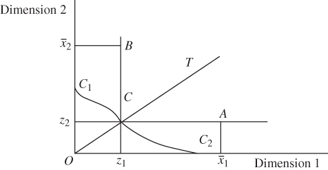
Figure 3.1 Identification of the poor.
The two one-dimensional poverty spaces ![]() and
and ![]() are displayed by the regions
are displayed by the regions ![]() and
and ![]() , respectively. While in the former region, a person is deprived in dimension 2, in the latter, deprivation arises from low achievement in dimension 1. The intersection of the two one-dimensional spaces generates the two dimensional space
, respectively. While in the former region, a person is deprived in dimension 2, in the latter, deprivation arises from low achievement in dimension 1. The intersection of the two one-dimensional spaces generates the two dimensional space ![]() . However, by summing up the numbers of individuals whose achievements lie inside the space, (
. However, by summing up the numbers of individuals whose achievements lie inside the space, (![]() ) will overestimate the number of poor. The reason behind is that the number of persons whose achievements lie inside
) will overestimate the number of poor. The reason behind is that the number of persons whose achievements lie inside ![]() is counted twice. Suppose that a person's achievements in the first
is counted twice. Suppose that a person's achievements in the first ![]() dimensions are zero and the achievement in the remaining dimension coincides with its threshold limit. This person is not counted as poor by the intersection method, however large or small the value of d may be. Thus, although the person is maximally deprived in all the dimensions except one and he is nondeprived in only one dimension, he is intersection nonpoor. This clearly indicates a shortcoming of the intersection rule as an identification criterion. Nevertheless, the union method identifies this person as poor.
dimensions are zero and the achievement in the remaining dimension coincides with its threshold limit. This person is not counted as poor by the intersection method, however large or small the value of d may be. Thus, although the person is maximally deprived in all the dimensions except one and he is nondeprived in only one dimension, he is intersection nonpoor. This clearly indicates a shortcoming of the intersection rule as an identification criterion. Nevertheless, the union method identifies this person as poor.
In the following discussion, we follow the union criterion of identification. This mechanism has installed itself as a notable identification criterion because of its easy implementation and long usage. For any ![]() ,
, ![]() , we denote the set of all poor persons in X by
, we denote the set of all poor persons in X by ![]() . For any given
. For any given ![]() , we write the number of poor persons in
, we write the number of poor persons in ![]() by
by ![]() . The head-count ratio, the proportion of persons in poverty, is
. The head-count ratio, the proportion of persons in poverty, is ![]() .
.
3.5 Axioms for a Multidimensional Poverty Metric
A multidimensional poverty index P is required to aggregate the deprivations of the individuals in a society along different dimensions of well-being in terms of a nonnegative scalar. For any vector of exogenously given threshold limits and an achievement matrix, this scalar signifies the extent of poverty related to the matrix. More precisely, it is a summary statistic of the distributions of individual deprivations in different dimensions of well-being. Unless specified explicitly, we assume that the set of all distribution matrices is given by ![]() . Then
. Then ![]() . For any
. For any ![]() , the scalar
, the scalar ![]() is the level of poverty associated with social matrix
is the level of poverty associated with social matrix ![]() , where
, where ![]() is arbitrary.
is arbitrary.
The structure of the current section, whose subject is the analysis of the properties for a multidimensional poverty index, parallels that of Part 2.3.1.1 of Section 2.3.1. Most of the postulates discussed next for an arbitrary P are generalizations of different postulates suggested for an income poverty index. However, any axiom that necessitates existence of at least two dimensions does not have any unidimensional sister.
3.5.1 Invariance Axioms
The axioms scrutinized in this subsection do not indicate any change in the extent of poverty when some allowable changes are made in achievement matrices.
The first of them indicates invariance of poverty if there are proportionate changes in the achievement quantities and threshold limits, where the proportionality factors may not be the same across dimensions.
- Strong Ratio-Scale Invariance: For all
 ,
,  , where
  ,
,  for all i.
To illustrate the axiom, consider the ![]() social matrix
social matrix  . Assume that the vector of threshold limits is given by
 ![]() . By the union rule of identification, the second, third, and fourth persons are poor. This is because each of these three persons is deprived in at least one dimension. While person 2 is deprived in dimensions 1 and 2, the only source of deprivation of person 3 is dimension 1. On the other hand, person 4 is deprived in all the three dimensions. The intersection mode, in contrast, will detect only the fourth person as poor.
. By the union rule of identification, the second, third, and fourth persons are poor. This is because each of these three persons is deprived in at least one dimension. While person 2 is deprived in dimensions 1 and 2, the only source of deprivation of person 3 is dimension 1. On the other hand, person 4 is deprived in all the three dimensions. The intersection mode, in contrast, will detect only the fourth person as poor.
Now, suppose that  so that
  and
and ![]() . Then strong ratio-scale invariance demands that
. Then strong ratio-scale invariance demands that  .
.
If the proportionality factors are assumed to be the same across dimensions, that is, if ![]() for all
for all ![]() , then we get the weaker form of the aforementioned axiom. We refer to this weaker variant of strong ratio-scale invariance as ratio-scale invariance, and a multidimensional poverty index satisfying this postulate will be known as a relative index. Evidently, all one-dimensional measures analyzed in Section 2.2 are of relative type.
, then we get the weaker form of the aforementioned axiom. We refer to this weaker variant of strong ratio-scale invariance as ratio-scale invariance, and a multidimensional poverty index satisfying this postulate will be known as a relative index. Evidently, all one-dimensional measures analyzed in Section 2.2 are of relative type.
Instead of assuming proportionate changes in achievement quantities, we can alternatively allow the possibility that these quantities can change by absolute amounts. More precisely, poverty will not change when dimensional achievement figures and threshold levels are changed by absolute quantities, where these absolute amounts may vary across dimensions. Formally,
- Strong Translation-Scale Invariance: For all
 ,
,  , where A is an
  matrix with identical rows given by
  such that
  and
and  for all
  .
.
For the ![]() translation matrix
translation matrix  , we have
  and
and ![]() . Consequently, strong translation-scale invariance claims that
. Consequently, strong translation-scale invariance claims that  . A weaker form of the postulate, translation-scale invariance axiom, requires that
 ![]() are not variable across dimensions. A poverty index satisfying this weaker axiom is called an absolute index.
are not variable across dimensions. A poverty index satisfying this weaker axiom is called an absolute index.
Sometimes, comparison between two societies with respect to their poverty levels becomes necessary. It is desirable that the poverty ranking remains unaltered even if the dimensional achievements and poverty cutoff limits in the two social matrices are expressed in differing measuring units. This requirement is ensured by the strong unit consistency axiom (Zheng, 2007a,b). To grasp the problem in greater detail, suppose that a policy-maker needs to rank social distributions of two countries in terms of their multidimensional poverty levels, where the dimensions included in the distributions are life expectancy and income. For illustrative purpose, assume that income is measured in dollar, and life expectancy is measured in years. It is noted that the former country has higher poverty compared to the latter. Now, if the policy-maker decides to change the measurement unit of income from dollar to euro and that of life expectancy from years to months, then strong unit consistency will require that the already observed poverty ranking should not alter as a consequence of these shifts in the measurement units of the dimensional achievements. Formally, the strong unit consistency axiom can be stated as:
- Strong Unit Consistency: For all
 and
and  , if
, if  , then
  for all
  = diag
  for all
  .
.
Evidently, all strongly ratio-scale invariant multidimensional poverty indices are strongly unit consistent. However, the converse is not true. More precisely, there may exist strongly unit-consistent multidimensional poverty indices that are not strongly ratio-scale invariant. If in the aforementioned axiom the positive scalars ![]() are the same across dimensions, then we refer to it as unit consistency.
are the same across dimensions, then we refer to it as unit consistency.
In the invariance axioms analyzed above we allow changes in all dimensional quantities, irrespective of whether they correspond to deprived or nondeprived dimensions. In the next two postulates, the focus axioms, changes only in nondeprived dimensional quantities are permitted. These two axioms were suggested by Bourguignon and Chakravarty (2003).12
Weak Focus: For all ![]() , if for some
, if for some ![]() ,
, ![]() for all
for all ![]() , for some pair
, for some pair ![]() ,
, ![]() , where
, where ![]() is a scalar such that
is a scalar such that ![]() and
and ![]() for all
for all ![]() , then
, then ![]() .
.
According to this postulate, for a rich person, who is not deprived in any dimension, a change in a dimensional quantity that does not make the person deprived in the dimension should not affect poverty. This is natural since poverty is concerned with the deprivations of the poor.
To illustrate this axiom, note that person 1 is nondeprived in all the three dimensions in X1. If we reduce his achievement quantity in dimension 3 from 90 to 80, then poverty should not change since the reduced quantity is much above the dimensional threshold limit, 50. If we denote the resulting distribution matrix by Y1, then  . The weak focus axioms stipulates that
 ![]() .
.
In the next axiom, we consider a change in a nondeprived dimensional achievement of a person such that the change does make the person deprived in the dimension. Formally,
- Strong Focus: For all
 , if for some pair
  ,
,  , where
  and
and  is a scalar such that
  and
and  for all
  , then
  .
.
Note that here in X1 the possibility that person i is poor is not excluded. This axiom has an interesting implication with respect to trade-off between nondeprived and deprived dimensional quantities of a poor person. When the level of achievement in a nondeprived dimension of a poor is reduced such that the resulting achievement quantity does not fall below the corresponding threshold limit, in exchange the person is not made better off in a deprived dimension. Consequently, trade-off between two dimensional achievements of a poor person who is deprived in one but nondeprived in the other is not possible. This definitely does not rule out potentiality of trade-off between two deprived dimensional quantities. The two focus axioms do not as well claim that the poverty index is independent of the nonpoor population size. (See Bourguignon and Chakravarty, 2003, for extensive discussions along this line.)
In X1 person 2 is nondeprived only in dimension 3 and hence he is poor by the union mode of identification. Now, the matrix  is obtained from X1 by reducing only person 2's achievement level in dimension 3 from 80 to 75 so that he is still nondeprived in the dimension. Then according to the strong focus axiom, this alteration does not change the quantity of overall poverty. More precisely,
 ![]() .
.
The reduction in achievement of the person in dimension 3 by 5 units is unable to reduce his deprivation in a deprived dimension.
The next two invariance axioms are poverty sisters of inequality symmetry and population replication invariance postulates, respectively.
- Symmetry: For all
 , if
, if  , where
  is any permutation matrix of order n, then
  .
. - Population Replication Invariance: For all
 ,
,  , where Y is any k-fold replication of X,
  being any finite integer.
Our discussions so far have been on axioms that do not allow any change in the poverty intensity under some specific type of alternations in an achievement matrix. Next, we analyze distributional axioms that indicate directional movements of a poverty index resulting from some transformations in a distribution matrix.
3.5.2 Distributional Axioms
Suppose that there is a curtailment in the achievement of a deprived dimension of a poor. Since such degradation in the achievement is undesirable from poverty reduction perspective, we can claim enhancement of poverty in this situation. In other words, a poverty index should increase under this state of affairs.
The following axiom addresses the impact of debasement in the attainment of a deprived dimension of a poor.
- Monotonicity: For all
 , if for some pair
  ,
,  , where
  ,
,  for all
  and
and  , then
  .
.
The social distribution  is deduced from X1 by a cutback of person 3's achievement in dimension 1, a deprived dimension for the person, by 1 unit. According to the monotonicity axiom,
 ![]() .
.
Often, it becomes desirable to ensure that a contraction in the achievement of a poor should increase poverty by a larger amount, the more deprived the person is. Similarly, an improvement in an achievement should lead to a greater diminution of poverty, the more deprived the poor is. This supports the view that the poorest subgroups in a society should receive maximum attention from antipoverty policy perspective. This plausible view is presented analytically in the next axiom (see Lasso de La Vega and Urrutia, 2012).
Let ![]() be the identical set of dimensions in which the poor persons i and h are deprived, that is,
be the identical set of dimensions in which the poor persons i and h are deprived, that is, ![]() , where
, where ![]() are arbitrary. Assume further that all deprivations of h are higher than the corresponding deprivations of i in
are arbitrary. Assume further that all deprivations of h are higher than the corresponding deprivations of i in ![]() . Formally, for all
. Formally, for all ![]() ,
, ![]() .
.
We assume that of two multidimensionally poor persons i and h, person h has higher deprivations than person i in some dimensions in X (condition (i)). Part (a) of condition (ii) states that in the three matrices X, Y, and ![]() , any person other than persons h and i has identical profile. Part (b) of the condition indicates that achievements in dimension j in Y and
, any person other than persons h and i has identical profile. Part (b) of the condition indicates that achievements in dimension j in Y and ![]() of persons h and i, respectively, are obtained by reducing the corresponding dimensional achievements in X by the same quantity, and this holds for all
of persons h and i, respectively, are obtained by reducing the corresponding dimensional achievements in X by the same quantity, and this holds for all ![]() . In part (c) of the condition, it is stated that achievements of each of the persons i and h in dimensions that are not in
. In part (c) of the condition, it is stated that achievements of each of the persons i and h in dimensions that are not in ![]() remain unaltered. In part (d) of the condition, it is claimed explicitly that amounts by which achievements of persons i and h in different dimensions in
remain unaltered. In part (d) of the condition, it is claimed explicitly that amounts by which achievements of persons i and h in different dimensions in ![]() are reduced are nonnegative and positive for some dimensions, and these amounts need not be the same across the dimensions. Finally, in part (e) of the condition, it is demanded that profiles of person i in X and Y are the same and those of person h are identical in X and
are reduced are nonnegative and positive for some dimensions, and these amounts need not be the same across the dimensions. Finally, in part (e) of the condition, it is demanded that profiles of person i in X and Y are the same and those of person h are identical in X and ![]() . Since
. Since ![]() , nonnegativity of achievement of person h in
, nonnegativity of achievement of person h in ![]() in any dimension in
in any dimension in ![]() is ensured.
is ensured.
We are now in a position to state the following axiom:
- Monotonicity Sensitivity: The poverty index
 satisfies the monotonicity sensitivity property.
This axiom says that we consider shrinkage in the achievements in dimensions in ![]() that applies identically to both i and h. The shrinkage operation is performed separately for the affected persons, and poverty increment is higher when it applies to the more deprived person h.
that applies identically to both i and h. The shrinkage operation is performed separately for the affected persons, and poverty increment is higher when it applies to the more deprived person h.
In X1, persons 2 and 4 are poor and both are deprived in dimensions 1 and 2. Person 2 has lower deprivation than person 4 in each of these dimensions. We get  and
and  from X1 by curtailing, respectively, the achievements of persons 2 and 4 in each of these dimensions by 1 unit. The monotonicity sensitivity axiom demands that
 ![]() .
.
The next axiom, suggested by Alkire and Foster (2011a), is concerned with the effect of increasing the number of deprived dimensions of a poor. It requires that when a nondeprived dimension of a poor person, who is not deprived in all dimensions, becomes deprived, then poverty should increase. Formally,
- Dimensional Monotonicity: For all
 , if
, if  is obtained from X such that for some pair
  ,
,  , where person i is deprived in X in at least dimension different from j and
  for all pairs
  , then
  .
.
Person i, who is poor and nondeprived in dimension j in X, becomes deprived in the dimension in Y. However, all other achievement levels for all persons in ![]() are the same in both X and Y. Now, under the change considered in the axiom, in Y, person i will be deprived in dimension j, a nondeprived dimension for the person in X. Hence, poverty should go up.
are the same in both X and Y. Now, under the change considered in the axiom, in Y, person i will be deprived in dimension j, a nondeprived dimension for the person in X. Hence, poverty should go up.
In our achievement matrix X1, dimension 2 is a nondeprived dimension for person 3, a poor person in X1. If his achievement in the dimension reduces from 6 to 4, he becomes deprived in this dimension in the transformed matrix  . Dimensional monotonicity axiom demands that
 ![]() .
.
Condition (i) ensures that there is at least one element in the alike set of deprived dimensions of the poor persons h and i. By assumption, of the two persons, the former has higher deprivations than the latter in this set. According to condition (ii), all individuals except persons h and i have identical achievements in all the dimensions in both X and Y. Part (a) of condition (iii) asserts that each of persons h and i has identical achievements in all dimensions that are not included in the set ![]() . Part (b) of condition (iii) means that transfers of achievements from person h to person i along dimensions in
. Part (b) of condition (iii) means that transfers of achievements from person h to person i along dimensions in ![]() generate appropriate entries of
generate appropriate entries of ![]() and
and ![]() from the corresponding entries of
from the corresponding entries of ![]() and
and ![]() , respectively, where the size of the transfer is nonnegative for any dimension in the set, and for at least one dimension of this type, the transfer has a positive size. Finally, in part (b) of condition (iii), it is ensured that the size of the transfer in any dimension does not allow the recipient to be nondeprived in the corresponding dimension. Since for any
, respectively, where the size of the transfer is nonnegative for any dimension in the set, and for at least one dimension of this type, the transfer has a positive size. Finally, in part (b) of condition (iii), it is ensured that the size of the transfer in any dimension does not allow the recipient to be nondeprived in the corresponding dimension. Since for any ![]() ,
, ![]() can at most be
can at most be ![]() , it is guaranteed that
, it is guaranteed that ![]() . The transfer operation takes place between the multidimensionally poor individuals i and h only in their common set of deprived dimensions. Equivalently, X is obtained from Y by a Pigou–Dalton bundle of progressive transfers.
. The transfer operation takes place between the multidimensionally poor individuals i and h only in their common set of deprived dimensions. Equivalently, X is obtained from Y by a Pigou–Dalton bundle of progressive transfers.
In the distribution matrix X1, ![]() , the identical set of deprived dimensions of persons 2 and 4, contains dimensions 2 and 1. Further, in each of these two dimensions, person 2 has higher achievement than person 4. Now, regressive transfers of 1 and 0.5 units of achievements in dimension 1 and 2, respectively, from person 4 to person 2, transform the matrix X1 into
, the identical set of deprived dimensions of persons 2 and 4, contains dimensions 2 and 1. Further, in each of these two dimensions, person 2 has higher achievement than person 4. Now, regressive transfers of 1 and 0.5 units of achievements in dimension 1 and 2, respectively, from person 4 to person 2, transform the matrix X1 into  . We then say that Y7 is deduced from X1 by a Pigou–Dalton bundle of regressive transfers between two persons.
The following transfer postulate for a multidimensional poverty index can now be stated.
- Multidimensional Transfer: For all
 ,
,  , if
, if  is obtained from X by a Pigou–Dalton bundle of regressive transfers between two multidimensionally poor persons, then
  .
.
This postulate may be regarded as a multidimensional translation of the Donaldson and Weymark (1986) weak transfer axiom. For the illustrative example, where we derive Y7 from X1 by a Pigou–Dalton bundle of regressive transfers between the multidimensionally poor persons 2 and 4, the transfer axiom demands that ![]() .
.
The final axiom in this subsection, we consider, has relevance only to multidimensional poverty and depends on the association between deprivations.
In Definition 3.3, conditions (i) and (ii) along with condition (iv) for ![]() and
and ![]() indicate that the multidimensionally poor person p who had less achievement in dimension j and more achievement in dimension q than the multidimensionally poor person i in X has higher achievements in both the dimensions in Y. It is also known that in all the remaining dimensions, achievements of person p are at least as high as the corresponding achievements of person i. Condition (iii) says that achievements for the remaining individuals in dimension j are the same in both the distribution matrices X and Y. Finally, condition (iv) demands that achievements of all persons in all the dimensions except j are the same in both the achievement matrices. We obtain Y from X by a switch of achievements in dimension j between persons i and p. In the postswitch setting, person p has at least as much achievement as person i in every dimension and strictly more in at least one dimension. Since both j and q are deprived dimensions for the poor persons i and p who are affected by the switch, we say that the switch is performed in a domain of deprivations. The switch of achievements in dimension j, defined by (i) and (ii), increases the correlation between dimensions. That is why, we refer to the switch as a correlation-increasing switch in a domain of deprivations. The switch does not modify the total of the achievements in the dimension on which it operates. In the two-dimensional situation, a correlation-increasing switch, as presented in Definition 3.3, holds only in the two-dimensional poverty space
indicate that the multidimensionally poor person p who had less achievement in dimension j and more achievement in dimension q than the multidimensionally poor person i in X has higher achievements in both the dimensions in Y. It is also known that in all the remaining dimensions, achievements of person p are at least as high as the corresponding achievements of person i. Condition (iii) says that achievements for the remaining individuals in dimension j are the same in both the distribution matrices X and Y. Finally, condition (iv) demands that achievements of all persons in all the dimensions except j are the same in both the achievement matrices. We obtain Y from X by a switch of achievements in dimension j between persons i and p. In the postswitch setting, person p has at least as much achievement as person i in every dimension and strictly more in at least one dimension. Since both j and q are deprived dimensions for the poor persons i and p who are affected by the switch, we say that the switch is performed in a domain of deprivations. The switch of achievements in dimension j, defined by (i) and (ii), increases the correlation between dimensions. That is why, we refer to the switch as a correlation-increasing switch in a domain of deprivations. The switch does not modify the total of the achievements in the dimension on which it operates. In the two-dimensional situation, a correlation-increasing switch, as presented in Definition 3.3, holds only in the two-dimensional poverty space ![]() .
.
If the two dimensions are substitutes, then one counterbalances the deficiency of the other. Since one person (person p), who was originally richer than the other person (person i) in dimension q, is becoming richer in the other dimension (dimension j) also after the switch and the two dimensions represent similar aspect of well-being, the switch should increase poverty. For the other person (person i), the inability to offset the shortage in one dimension by the other now increases because he is now poorer in both the dimensions.
The aforementioned discussion enables us to state the following axiom:
- Increasing Poverty under Correlation-Increasing Switch: For all
 , if Y is obtained from X by a correlation-increasing switch in a domain of deprivations, then
  if the dimensions involved in the switch are substitutes.
The corresponding postulate when the dimensions are complements requires poverty to decrease under such a switch. The switch will not affect poverty at all if the involved dimensions are independents.
3.5.3 Decomposability Axioms
A decomposability postulate deals with disaggregation of a poverty index by employing some well-defined procedure. They are helpful in monitoring poverty, targeting poor people, and implementing antipoverty policies. According to the first of these, subgroup decomposability, for any attribute-dependent split-up of the population into two or more subgroups, overall poverty can be expressed as the weighted average of subgroup poverty levels, where the weights are population shares of respective subgroups. (See Chapter 2 for a related discussion in the context of inequality.)
Formally,
- Subgroup Decomposability: For any
 and
and  ,
,  , where
  , ni is the population size associated with Xi and
  .
.
To understand this, suppose that the population has been broken down into l subgroups using region as a social characteristic. Then Xi is the distribution matrix of region i, ![]() is the corresponding poverty level,
is the corresponding poverty level, ![]() is the proportion of the total population belonging to this region, and
is the proportion of the total population belonging to this region, and ![]() is the level of overall poverty, that is, the extent of poverty that arises when all the regions are taken together. Under repeated application of subgroup decomposability, we have
is the level of overall poverty, that is, the extent of poverty that arises when all the regions are taken together. Under repeated application of subgroup decomposability, we have  . Population poverty becomes disaggregated as the average of individual poverty levels. Since
 ![]() depends only on individual i's achievement profile, it is often referred to as individual poverty function.
depends only on individual i's achievement profile, it is often referred to as individual poverty function.
The breakdown  clearly establishes that a subgroup-decomposable poverty index is population replication invariant and symmetric. But the converse is not true.
For illustrative purpose, consider again the four-person distribution matrix X1. Assume that the population has been divided into two subgroups using sex as the characteristic of division. Let the submatrices  and
and  denote respectively the distribution matrices of the female and male populations. Then under the assumption that the threshold limit vector is given by
 ![]() , subgroup decomposability requires that
, subgroup decomposability requires that ![]() .
.
This type of breakdown of population poverty enables us to evaluate the impact of subgroup poverty levels on overall poverty. In other words, one can determine the contribution of a subgroup's poverty to total poverty. Analytically, the contribution of subgroup i to global poverty is ![]() . Such contributions made by different subgroups become helpful in isolating subgroups that are more stressed by multidimensional poverty and hence to implement antipoverty at local levels. Some of the subgroups get identified as highly contributing subgroups because of large population proportions although their poverty levels are low. In contrast, there may be subgroups with low population shares but high poverty levels so that they are treated as high-poverty-contributing subgroups. This should be kept in mind while implementing the underlying targeted poverty alleviation policy. More precisely, subgroups with low population fractions and high poverty levels should be primary targets from antipoverty policy perspective. Given that population poverty turns out to be the average of individual poverty levels, determination of individual contributions is possible, which sometimes may be useful. This is certainly true when the community population size is not very high, and we are concentrating on household poverty levels.
. Such contributions made by different subgroups become helpful in isolating subgroups that are more stressed by multidimensional poverty and hence to implement antipoverty at local levels. Some of the subgroups get identified as highly contributing subgroups because of large population proportions although their poverty levels are low. In contrast, there may be subgroups with low population shares but high poverty levels so that they are treated as high-poverty-contributing subgroups. This should be kept in mind while implementing the underlying targeted poverty alleviation policy. More precisely, subgroups with low population fractions and high poverty levels should be primary targets from antipoverty policy perspective. Given that population poverty turns out to be the average of individual poverty levels, determination of individual contributions is possible, which sometimes may be useful. This is certainly true when the community population size is not very high, and we are concentrating on household poverty levels.
The objective of the second decomposability postulate, factor decomposability, is to assess the contributions of individual dimensions to overall poverty. In other words, it enables us to identify the causal factors of poverty using dimension-by-dimension breakdown. Formally,
- Factor Decomposability: For all
 ,
,  ,
,  , where
  for all
  and
and  .
.
In other words, overall poverty is the weighted average of dimensional poverty values, where the weight attached to each of the dimensional poverty levels is positive (Chakravarty et al. 1998). This postulate may be regarded as the poverty counterpart to the inequality factor decomposability axiom proposed in Chapter 2. The weight ![]() allotted to dimension j's poverty may be interpreted as the importance a policy-maker assigns to the role of the dimension in poverty assessment. The weights may depend on achievement distributions. We may as well follow the normative criterion of assigning equal weight to the dimensional indices so that
allotted to dimension j's poverty may be interpreted as the importance a policy-maker assigns to the role of the dimension in poverty assessment. The weights may depend on achievement distributions. We may as well follow the normative criterion of assigning equal weight to the dimensional indices so that ![]() for all
for all ![]() (see Chapter 1).
(see Chapter 1).
The contribution of weighted poverty in dimension j to overall poverty turns out to be ![]() . This contribution reduces to 0 if nobody is deprived in the dimension. We are following here the union poverty criterion. Alternatively, if we choose the intersection poverty rule, then for positivity of contribution of a dimensional poverty, it is necessary that everybody is deprived in the dimension. Each of these dimensionwise statistics is important from policy perspective since using them we can judge which dimensions are contributing more. This is especially attractive for designing antipoverty policy at dimension levels.
. This contribution reduces to 0 if nobody is deprived in the dimension. We are following here the union poverty criterion. Alternatively, if we choose the intersection poverty rule, then for positivity of contribution of a dimensional poverty, it is necessary that everybody is deprived in the dimension. Each of these dimensionwise statistics is important from policy perspective since using them we can judge which dimensions are contributing more. This is especially attractive for designing antipoverty policy at dimension levels.
A factor-decomposable poverty index is a composite index; it assembles the components of the dimensional dashboard ![]() using the positive weights
using the positive weights ![]() assigned across dimensions in
assigned across dimensions in  . Consequently, a multidimensional poverty index satisfying the factor decomposability postulate is insensitive to a correlation-increasing switch.
Often, a country's budget for elimination of poverty from one highly contributing subgroup or from one highly contributing dimension for the population as a whole may not be sufficient. In such a case, identification of the highly contributing dimension within a highly contributing subgroup may be appropriate, given that the allocated budget is sufficient to eliminate poverty associated with this (subgroup, dimension) combination.
Analytically, suppose that in a population partitioned into l subgroups, ![]() , the contribution of subgroup k is the highest among the subgroups. The source of this high contribution is a very high value of the subgroup poverty
, the contribution of subgroup k is the highest among the subgroups. The source of this high contribution is a very high value of the subgroup poverty ![]() although
although ![]() , the population fraction of the subgroup, is rather low. Consequently, from antipoverty policy perspective, elimination of poverty from this subgroup should get top priority. However, the limited allocated budget does not enable the administration to perform the job. Evidently, in such a case, identification of the highest contributing dimension within this subgroup is necessary.
, the population fraction of the subgroup, is rather low. Consequently, from antipoverty policy perspective, elimination of poverty from this subgroup should get top priority. However, the limited allocated budget does not enable the administration to perform the job. Evidently, in such a case, identification of the highest contributing dimension within this subgroup is necessary.
Note that under factor decomposability, we can split ![]() into dimensionwise components as
into dimensionwise components as ![]() , where
, where ![]() is the jth column of the distribution matrix Xk, indicating the distribution of achievements in dimension
is the jth column of the distribution matrix Xk, indicating the distribution of achievements in dimension ![]() in Xk. Now, suppose that among all the components of
in Xk. Now, suppose that among all the components of ![]() ,
, ![]() assumes the highest value. Formally,
assumes the highest value. Formally, ![]() . In other words, among all dimensionwise components of
. In other words, among all dimensionwise components of ![]() , the maximum contributor turns out to be
, the maximum contributor turns out to be ![]() , poverty arising from distribution of achievements in dimension p in Xk. Consequently, the subgroup–dimension combination that deserves maximum attention from poverty alleviation perspective is
, poverty arising from distribution of achievements in dimension p in Xk. Consequently, the subgroup–dimension combination that deserves maximum attention from poverty alleviation perspective is ![]() . If poverty is eliminated from this subgroup–dimension combination, then overall poverty reduces by the quantity
. If poverty is eliminated from this subgroup–dimension combination, then overall poverty reduces by the quantity ![]() .
.
An illustration will make the idea clearer. Assume that in the decomposition of ![]() by sex,
by sex, ![]() . Assume further that among the three dimensionwise components
. Assume further that among the three dimensionwise components  ,
,  and
and  of
of ![]() , the highest contribution comes from
, the highest contribution comes from  . More precisely,
 . This in turn enables us to conclude that the (subgroup–dimension) pair that requires maximum attention from poverty remedial point of view is (male, 1).
3.5.4 Threshold Limit Sensitivity Axiom
The axioms stated so far assume constancy of threshold limits. However, sometimes, a policy-maker may recommend revision of one or more threshold limits, say, following some steady changes in the prices of the achievements in the corresponding dimensions. In such a case, it becomes necessary to investigate how the level of existing poverty alters under such changes.
- Nondecreasingness in Poverty Thresholds: For all
 , let
, let  be such that
  for some
  ,
,  . Then
  .
.
If a dimension is already deprived for some individuals, then an increase in its threshold limit can lead to increase in dimensional deprivations of these persons. Further, newer persons may become deprived. Consequently, multidimensional poverty may increase. In the society with the social distribution ![]() and vector of poverty cutoff points
and vector of poverty cutoff points ![]() , suppose that the cutoff limit in dimension 3 increases from 50 to 60, then person 3 who was nondeprived originally in the dimension becomes deprived. Further, person 4's deprivation in the dimension deepens. Consequently, it is legitimate to claim that
, suppose that the cutoff limit in dimension 3 increases from 50 to 60, then person 3 who was nondeprived originally in the dimension becomes deprived. Further, person 4's deprivation in the dimension deepens. Consequently, it is legitimate to claim that ![]() .
.
The final subsection of this section deals with two technical postulates. The first of these, boundedness, is a cardinality principle. This axiom says that if nobody is deprived in any dimension, then the index takes on the minimum value 0. In other words, the poverty index achieves its lower bound 0 if nobody is deprived in any dimension. In particular, in a subgroup-decomposable index, if for a nonpoor person, who is nondeprived in all dimensions, the associated individual poverty function assumes the value 0, then the index achieves this lower bound.
On the other hand, the upper bound 1 is achieved if everybody's deprivation is maximal in each dimension. Maximal deprivation for each person in each dimension is a sensible requirement for a poverty index to reach its upper bound. It is a cardinality principle because we can also make the poverty index bounded in some other interval of the set of real numbers by taking an affine transformation of the index. The second property, continuity, requires that there should not be any sudden upward or downward movements of the poverty index for small changes in the deprived achievement levels, under ceteris paribus conditions. Rather, the poverty quantity should change by a negligible amount in this scenario.
3.5.5 Technical Axioms
- Boundedness: For all
 ,
,  ,
,  ,
,  is bounded between 0 and 1, where the lower bound is attained if
  is such that
  , the set of poor persons in X, is empty. The upper bound is attained if everybody is maximally deprived in each dimension.
 - Continuity: For all
 ,
,  , P varies continuously with respect to changes in achievements of the poor, provided that the poverty statuses of the individuals are not affected as a result of achievement variations.
We now study an interesting implication of some of the postulates analyzed earlier. This property indicates a particular directional change in poverty resulting from an increase in nonpoor population size. For any ![]() , consider
, consider  , where
 ![]() is the achievement profile of the
is the achievement profile of the ![]() person in
person in ![]() and
and ![]() for all
for all ![]() . In other words, X is obtained from Y by adding a rich person to the society. Suppose that P is subgroup decomposable and achieves the lower bound 0 in the situation described in the axiom. Now,
. In other words, X is obtained from Y by adding a rich person to the society. Suppose that P is subgroup decomposable and achieves the lower bound 0 in the situation described in the axiom. Now,  . Since the
 ![]() person is not deprived in any dimension,
person is not deprived in any dimension, ![]() . In consequence, it follows that
. In consequence, it follows that  . This demonstration claims that if a rich person migrates to the society, then a subgroup-decomposable poverty index achieving the lower bound 0 for a society with nonpoor persons will indicate lower poverty for the enlarged society than for the original one.
To understand the property explicitly, suppose that a person with achievement profile ![]() migrates to the four-person society whose social matrix is X1. This person is nonpoor. Hence,
migrates to the four-person society whose social matrix is X1. This person is nonpoor. Hence, ![]() . We denote the resulting social matrix by Y8 so that
. We denote the resulting social matrix by Y8 so that  . The property then demands that under subgroup decomposability,
 ![]() . We can refer to this property of a multidimensional poverty index as nonpoverty population growth axiom.
. We can refer to this property of a multidimensional poverty index as nonpoverty population growth axiom.
3.6 Multidimensional Poverty Measurement
In this section, we analyze some functional forms for multidimensional poverty indices. Each of these functional specifications is a summary statistic of deprivations of the poor along different dimensions of well-being in terms of a real number. We begin by presenting dashboard-based composite indices. Next, we discuss the direct approach, the main method adopted in the literature, in which axioms and poverty measures are defined directly on multidimensional matrices (see also Duclos and Tiberti, 2016). We then turn to the indices that can be interpreted from the inclusive measure of well-being perspective.
3.6.1 The Dashboard Approach
The example we consider in this subsection is based on a dashboard of dimensional indices. For any ![]() ,
, ![]() ,
, ![]() signifies the level of poverty associated with
signifies the level of poverty associated with ![]() , the distribution of achievements in dimension j. (Unless stated, the assumption
, the distribution of achievements in dimension j. (Unless stated, the assumption ![]() will be maintained throughout the section.) The
will be maintained throughout the section.) The ![]() dimensional poverty dashboard is given by
dimensional poverty dashboard is given by ![]() . For illustrative purpose, assume that the dimensional metrics are given by
. For illustrative purpose, assume that the dimensional metrics are given by  , where
 ![]() is arbitrary and the transformation
is arbitrary and the transformation ![]() satisfies
satisfies ![]() . Since
. Since ![]() indicates person i's deprivation in dimension j,
indicates person i's deprivation in dimension j, ![]() is the corresponding transformed deprivation indicator. It is also assumed to be decreasing, continuous, and strictly convex in the concerned dimensional achievements of the poor. Each of the d dimensional metrics is the arithmetic average of transformed deprivations in the dimension. The resulting dashboard then becomes
is the corresponding transformed deprivation indicator. It is also assumed to be decreasing, continuous, and strictly convex in the concerned dimensional achievements of the poor. Each of the d dimensional metrics is the arithmetic average of transformed deprivations in the dimension. The resulting dashboard then becomes  . Evidently,
 ![]() if nobody is deprived in dimension j.
if nobody is deprived in dimension j.
Decreasingness of ![]() ensures that a reduction in the achievement of a poor person in any deprived dimension
ensures that a reduction in the achievement of a poor person in any deprived dimension ![]() increases
increases ![]() . Strict convexity of
. Strict convexity of ![]() guarantees that a transfer of achievement from a poor person to a richer poor person such that the poverty status of the recipient does not change increases
guarantees that a transfer of achievement from a poor person to a richer poor person such that the poverty status of the recipient does not change increases ![]() , where the deprived dimension
, where the deprived dimension ![]() is arbitrary. This implies that if each component
is arbitrary. This implies that if each component ![]() of the dashboard
of the dashboard  is increasingly related to the composite poverty index to be designed from the dashboard, then the underlying composite index satisfies the Bourguignon and Chakravarty (2003) one-dimensional transfer principle. The one-dimensional transfer principle necessitates a raise of multidimensional poverty under a regressive transfer of achievement in a deprived dimension from a poorer poor to a richer poor, given that the poverty status of the richer person, achievements of the two affected persons in all other dimensions, and achievements of all the remaining persons are kept unchanged.
Sequential applications of one-dimensional transfers miss the essence of multidimensionality and hence are not suitable in the current context. The appropriate notion of redistribution is the multidimensional transfer axiom.
An extremely simple way to arrive at a composite index is to take a weighted average of dimensional indices incorporated into the dashboard. Formally, the formula for the composite index turns out to be

which can alternatively be expressed as

where ![]() is the weight assigned to poverty assessed in dimension j,
is the weight assigned to poverty assessed in dimension j,  . Chakravarty et al. (1998) suggested (3.7a) assuming subgroup decomposability and factor decomposability at the outset. But it emerges that
 ![]() in (3.7a) can also be accommodated within the dashboard framework.
in (3.7a) can also be accommodated within the dashboard framework.
By assigning positive weights to individual dimensional poverty amounts in the dashboard, we implicitly assume that all the dimensions are important in global poverty evaluation. However, any choice of the weights will reflect a particular value judgment. (See Section 1.5 for a discussion. See also Aaberge and Brandolini, 2015.) For instance, if we choose ![]() , then all the dimensions are marked as equally important.
, then all the dimensions are marked as equally important.
By construction, the symmetric, population replication invariant, dashboard-based family ![]() satisfies monotonicity. It as well satisfies monotonicity sensitivity and dimensional monotonicity axioms. It expands if the threshold limit of a dimension in which there is at least one deprived person goes up. Although it verifies the multidimensional transfer principle, it does not change under a correlation-increasing switch and hence treats the dimensions as “independents.”
satisfies monotonicity. It as well satisfies monotonicity sensitivity and dimensional monotonicity axioms. It expands if the threshold limit of a dimension in which there is at least one deprived person goes up. Although it verifies the multidimensional transfer principle, it does not change under a correlation-increasing switch and hence treats the dimensions as “independents.”
Several members of the family (3.7) are worthy of investigation. For the transformation ![]() , where
, where ![]() , the underlying measuring instrument becomes the Watts (1968) index of multidimensional poverty:
, the underlying measuring instrument becomes the Watts (1968) index of multidimensional poverty:

In order to develop a characterization of this index, Tsui (2002) assumed in the first place that a poverty index is symmetric, population replication invariant, strongly focussed, monotonic, and continuous in achievements. He then demonstrated that axioms of strong ratio-scale invariance, decreasingness under a uniform majorization operation among the poor, nondecreasingness with respect to a correlation-increasing switch among the poor, subgroup consistency, and poverty criterion invariance hold together if and only if ![]() is one of the members of a two-member family. Subgroup consistency requires that for any partitioning of the population into two or more subgroups, if poverty in one subgroup goes down and stays fixed in the other subgroups, then global poverty should reduce as well (see Foster and Shorrocks, 1991). Poverty criterion invariance demands that there should be no change in poverty ranking if one or more threshold limits change, keeping the number of poor unaltered.
is one of the members of a two-member family. Subgroup consistency requires that for any partitioning of the population into two or more subgroups, if poverty in one subgroup goes down and stays fixed in the other subgroups, then global poverty should reduce as well (see Foster and Shorrocks, 1991). Poverty criterion invariance demands that there should be no change in poverty ranking if one or more threshold limits change, keeping the number of poor unaltered.
Chakravarty and Silber (2008) characterized this index from a welfare theoretic perspective. Poverty index is defined as welfare loss generated as a consequence of shortfall of dimensional achievements of the poor from the respective cutoff limits. It was then demonstrated that the only strongly focused poverty index satisfying subgroup decomposability, strong ratio-scale invariance, montonicity, and continuity in achievements is ![]() .
.
An attractive feature of the Watts index is that we can split up the change in poverty between two periods into its multidimensional growth and multidimensional redistribution components (see Chakravarty et al., 2008). Inquiry concerning relationships among poverty, economic growth, and inequality is highly motivated by policy-related issues including “trickle-down” eventualities of economic growth and impact of structural adjustment plans for stabilizing the economy (See, e.g., Ravallion and Huppi, 1991; Datt and Ravallion, 1992; Kakwani 1993 and Lipton and Ravallion, 1995.) To diagnose the growth and redistribution ingredients explicitly, suppose that ![]() and
and ![]() stand for the achievement matrices of a society in periods 1 and 2, and let the corresponding population sizes be
stand for the achievement matrices of a society in periods 1 and 2, and let the corresponding population sizes be ![]() and
and ![]() , respectively. Then assuming that the threshold limits stay put, the poverty change between the two periods happens to be
, respectively. Then assuming that the threshold limits stay put, the poverty change between the two periods happens to be

where ![]() stands for the mean of the jth dimensional achievements of the poor in period t (t = 1, 2). The first third bracketed term on the right-hand side of (3.10) represents the redistribution factor showing the change in poverty resulting from a change in inequality among the poor, given that the means of their dimensional achievements stay put. The inequality index that appears here is a member of the multidimensional generalized entropy family (see Equation (2.9c)). It is a multidimensional extension of Theil's mean logarithmic deviation (see Equation (2.8)). The second third bracketed term of the right-hand expression is the growth ingredient of the decomposition. It signifies the change in the poverty that follows from changes in means of achievements of the poor under the a priori assumption that inequality stays fixed (see also Chakravarty, 2009). It shows the effectiveness of economic growth on poverty change.13
stands for the mean of the jth dimensional achievements of the poor in period t (t = 1, 2). The first third bracketed term on the right-hand side of (3.10) represents the redistribution factor showing the change in poverty resulting from a change in inequality among the poor, given that the means of their dimensional achievements stay put. The inequality index that appears here is a member of the multidimensional generalized entropy family (see Equation (2.9c)). It is a multidimensional extension of Theil's mean logarithmic deviation (see Equation (2.8)). The second third bracketed term of the right-hand expression is the growth ingredient of the decomposition. It signifies the change in the poverty that follows from changes in means of achievements of the poor under the a priori assumption that inequality stays fixed (see also Chakravarty, 2009). It shows the effectiveness of economic growth on poverty change.13
A multidimensional generalization of the one-dimensional Chakravarty (1983) index was suggested by Chakravarty et al. (1998) entailing additivity over transformed individual dimensional deprivations. It corresponds to the transformation ![]() , where
, where ![]() is a constant. The resulting summary measure becomes
is a constant. The resulting summary measure becomes

For any value of ![]() , the index satisfies the monotonicity sensitivity property. For
, the index satisfies the monotonicity sensitivity property. For ![]() , overall poverty assumes the form of weighted average of dimensional deprivations of an average person. Although the transfer principle is violated in this case, it may be worthwhile to note that for computational purpose, we only need information on dimensionwise deprivations of different individuals and the dimensional weights.
, overall poverty assumes the form of weighted average of dimensional deprivations of an average person. Although the transfer principle is violated in this case, it may be worthwhile to note that for computational purpose, we only need information on dimensionwise deprivations of different individuals and the dimensional weights.
Finally, consider the specification ![]() , where
, where ![]() is a parameter. The consequential multidimensional index comes out to be
is a parameter. The consequential multidimensional index comes out to be

This is a simple multidimensional extension of the Foster–Greer–Thorbecke unidimensional index (see Foster et al., 1984). It satisfies the monotonicity sensitivity axiom for all ![]() . The values
. The values ![]() and
and ![]() coincide when
coincide when ![]() .
.
3.6.2 The Direct Approach
The first example we provide in this subsection is the second member of the Tsui (2002) family, defined as

where ![]() is arbitrary and the parameters
is arbitrary and the parameters ![]() are positive for all
are positive for all ![]() . The subscript
. The subscript ![]() indicates that this strongly relative (more generally, strongly ratio-scale invariant) index was proposed by Tsui, and
indicates that this strongly relative (more generally, strongly ratio-scale invariant) index was proposed by Tsui, and ![]() stands for the d dimensional vector of parameters
stands for the d dimensional vector of parameters ![]() . This quantifier of poverty is an alternative multivariate extension of the one-dimensional Chakravarty (1983) index. (See Eq. (3.1)). While the first member of the Tsui family involves additive aggregation both across dimensions and across individuals, in (3.12), a multiplicative aggregation across dimensions is employed. The parameters
. This quantifier of poverty is an alternative multivariate extension of the one-dimensional Chakravarty (1983) index. (See Eq. (3.1)). While the first member of the Tsui family involves additive aggregation both across dimensions and across individuals, in (3.12), a multiplicative aggregation across dimensions is employed. The parameters ![]() have to obey some inequality restrictions for the fulfillment of different axioms. For
have to obey some inequality restrictions for the fulfillment of different axioms. For ![]() , verification of the transfer axiom is ensured by the restrictions
, verification of the transfer axiom is ensured by the restrictions ![]() and
and ![]() . It is unambiguously increasing with reference to a correlation-increasing switch.
. It is unambiguously increasing with reference to a correlation-increasing switch.
The next proposal we wish to analyze is the Bourguignon and Chakravarty (2003) index ![]() , one of the most widespread indices of multidimensional poverty:
, one of the most widespread indices of multidimensional poverty:

where the parameters α and θ are positive, and ![]() is the weight assigned to the transformed deprivation indicator
is the weight assigned to the transformed deprivation indicator ![]() of dimension j,
of dimension j,  . Accordingly, the individual poverty function
  in (3.13) is obtained by raising the weighted average of such indicators across dimensions to the power
 ![]() . Multidimensional poverty is then defined as the simple arithmetic average of individual poverty functions. As a consequence, by construction, the index comes to be subgroup decomposable (hence symmetric and population replication invariant). Further, it is continuous, bounded, strongly ratio-scale invariant, and dimensionally monotonic. It also gladdens the monotonicity sensitivity (hence monotonicity) and threshold limit sensitivity axioms. The transfer axiom is satisfied when θ is greater than 1. For a given θ, as the value of α increases, sensitivity of dimensionwise regressive transfers at lower down the distributions of achievements increases. It may be viewed as a simple parametric generalization of the Foster et al. (1984) one-dimensional index to the multidimensional framework.
. Multidimensional poverty is then defined as the simple arithmetic average of individual poverty functions. As a consequence, by construction, the index comes to be subgroup decomposable (hence symmetric and population replication invariant). Further, it is continuous, bounded, strongly ratio-scale invariant, and dimensionally monotonic. It also gladdens the monotonicity sensitivity (hence monotonicity) and threshold limit sensitivity axioms. The transfer axiom is satisfied when θ is greater than 1. For a given θ, as the value of α increases, sensitivity of dimensionwise regressive transfers at lower down the distributions of achievements increases. It may be viewed as a simple parametric generalization of the Foster et al. (1984) one-dimensional index to the multidimensional framework.
Its value increases or decreases under a correlation-increasing switch depending on whether α is greater or less than θ. As a result, while under the restriction ![]() , the dimensions affected by the switch are treated as substitutes, they are counted as complements whenever the reverse restriction
, the dimensions affected by the switch are treated as substitutes, they are counted as complements whenever the reverse restriction ![]() holds. That is why,
holds. That is why, ![]() is referred to as the “Bourguignon–Chakravarty substitutes” index for
is referred to as the “Bourguignon–Chakravarty substitutes” index for ![]() , and it is known as the “Bourguignon–Chakravarty complements” index for
, and it is known as the “Bourguignon–Chakravarty complements” index for ![]() (Vélez and Robles, 2008, p. 217).
(Vélez and Robles, 2008, p. 217).
For ![]() ,
, ![]() coincides with
coincides with ![]() in (3.11) and hence gets converted into a composite index, which shows insensitivity to a correlation-increasing switch. Bourguignon and Chakravarty (2003) proposed and analyzed this index extensively by assuming that the deprivation indicator of person i in dimension j is given by
in (3.11) and hence gets converted into a composite index, which shows insensitivity to a correlation-increasing switch. Bourguignon and Chakravarty (2003) proposed and analyzed this index extensively by assuming that the deprivation indicator of person i in dimension j is given by ![]() , where
, where ![]() for all
for all ![]() , and they need not be the same across dimensions. The resulting index, which Alkire et al. (2015) denoted as
, and they need not be the same across dimensions. The resulting index, which Alkire et al. (2015) denoted as ![]() , comes to be
, comes to be  . We can as well obtain it by assuming first parametric variability in
 ![]() . More precisely, first α is replaced by αj and θ is replaced by
. More precisely, first α is replaced by αj and θ is replaced by ![]() where
where ![]() is arbitrary, and variability of these 2d such parameters across dimensions is allowed. At the second step, we assume that
is arbitrary, and variability of these 2d such parameters across dimensions is allowed. At the second step, we assume that ![]() for all
for all ![]() and deduce
and deduce ![]() . Alkire et al. (2015) refer to
. Alkire et al. (2015) refer to ![]() , which is known in the literature as the Bourguignon–Chakravarty index, as
, which is known in the literature as the Bourguignon–Chakravarty index, as ![]() . For α = 1, θ = 1, the value of
. For α = 1, θ = 1, the value of ![]() matches with those of
matches with those of ![]() and
and ![]() when
when ![]() , indicating its insensitivity to a correlation-increasing swap as well as transfers.
, indicating its insensitivity to a correlation-increasing swap as well as transfers.
The parameter θ is directly related to the curvature of an isopoverty contour, a locus of achievements in ![]() that generate the same value of the individual poverty function. For any
that generate the same value of the individual poverty function. For any ![]() , an isopoverty contour becomes strictly convex to the origin. As the value of θ over the interval
, an isopoverty contour becomes strictly convex to the origin. As the value of θ over the interval ![]() rises, convexity of the contour increases under ceteris paribus assumptions. Because of this, the marginal rate of substitution, the trade-off between the proportionate deprivations in the given dimensions, becomes increasingly difficult with an increase in the value of θ.
rises, convexity of the contour increases under ceteris paribus assumptions. Because of this, the marginal rate of substitution, the trade-off between the proportionate deprivations in the given dimensions, becomes increasingly difficult with an increase in the value of θ.
The constant elasticity of substitution between proportionate shortfalls associated with the two dimensions is ![]() . For θ = 1, there is perfectly elastic trade-off between the proportionate deprivations; the isopoverty contour becomes a straight line in this polar situation. At the other extreme, as
. For θ = 1, there is perfectly elastic trade-off between the proportionate deprivations; the isopoverty contour becomes a straight line in this polar situation. At the other extreme, as ![]() , we get the rectangular isopoverty contour.
, we get the rectangular isopoverty contour.
Given α, in the limit as ![]() ,
, ![]() approaches
approaches

As the two-dimensional individual isopoverty curves corresponding to the formula (3.14) are of rectangular shape, substitution between the two relative shortfalls is ruled out. The information required for this representation of multidimensional poverty is rather basic; knowledge of the proportionate shortfalls is sufficient to perform the underlying aggregation. (See Bourguignon and Chakravarty, 1999, for further discussion.) In consideration of the fact that ![]() in (3.14) employs a Leontief-type aggregation, Vélez and Robles (2008, p. 217) refer to it as the “Bourguignon–Chakravarty–Leontief” index. The second expression of (3.14) clearly demonstrates that in this limiting case,
in (3.14) employs a Leontief-type aggregation, Vélez and Robles (2008, p. 217) refer to it as the “Bourguignon–Chakravarty–Leontief” index. The second expression of (3.14) clearly demonstrates that in this limiting case, ![]() is the average of the relative maximin individual poverty functions.
is the average of the relative maximin individual poverty functions.
Bourguignon and Chakravarty (2003) considered extensions of ![]() in (3.13) by allowing variation of the elasticity of substitution between dimensional proportionate shortfalls with the level of poverty. For instance, if a person is highly deprived in one dimension but is characterized with a very low level of deprivation in a second dimension, then elasticity of substitution may be of minor significance. This is because deprivation in the first dimension becomes a major determinant of overall poverty. But if the extents of deprivations are low in both the dimensions, then the roles of deprivations in both the dimensions are important. One may assume the opposite as well; scope of substitution decreases with the level of poverty. These two positions can be incorporated into the general Bourguignon–Chakravarty index (3.13) by assuming that the parameter θ depends on the level of poverty. More precisely, we replace θ in (3.13) by
in (3.13) by allowing variation of the elasticity of substitution between dimensional proportionate shortfalls with the level of poverty. For instance, if a person is highly deprived in one dimension but is characterized with a very low level of deprivation in a second dimension, then elasticity of substitution may be of minor significance. This is because deprivation in the first dimension becomes a major determinant of overall poverty. But if the extents of deprivations are low in both the dimensions, then the roles of deprivations in both the dimensions are important. One may assume the opposite as well; scope of substitution decreases with the level of poverty. These two positions can be incorporated into the general Bourguignon–Chakravarty index (3.13) by assuming that the parameter θ depends on the level of poverty. More precisely, we replace θ in (3.13) by ![]() , a positive-valued function of the extent of poverty P. The consequential variant of
, a positive-valued function of the extent of poverty P. The consequential variant of ![]() in (3.13) that emerges under this assumption about the value of θ is
in (3.13) that emerges under this assumption about the value of θ is

Two simple forms of ![]() that will ensure decreasingness and increasingness of the elasticity of substitution as poverty level increases are, respectively,
that will ensure decreasingness and increasingness of the elasticity of substitution as poverty level increases are, respectively, ![]() and
and ![]() . (P here stands for
. (P here stands for ![]() and hence is bounded so that the examples of
and hence is bounded so that the examples of ![]() we have considered are well defined.) Under these specifications of
we have considered are well defined.) Under these specifications of ![]() , we can solve equation (3.15) numerically. The variant (3.15) of (3.13) inherits all postulates of the original poverty representation (3.13), except unambiguous change under a correlation-increasing swap between two poor persons. The swap may increase or decrease overall poverty depending on whether the affected persons are very poor or moderately poor.
, we can solve equation (3.15) numerically. The variant (3.15) of (3.13) inherits all postulates of the original poverty representation (3.13), except unambiguous change under a correlation-increasing swap between two poor persons. The swap may increase or decrease overall poverty depending on whether the affected persons are very poor or moderately poor.
In their excellent contributions, Lasso de la Vega and Urrutia (2011, 2009) characterized ![]() axiomatically as a multidimensional deprivation index by employing several intuitively understandable axioms defined on the set of deprivations of the individuals in different dimensions of well-being. The set of axioms invoked in the characterization includes continuity, monotonicity, weak dimension separability, homotheticity, subgroup decomposability, and normalization. The first axiom, continuity, stresses continuous variation in the index with respect to its arguments. The next axiom, monotonicity, says that overall deprivation is increasing with respect to dimensionwise deprivations. The third axiom, weak dimension separability, requires that for any separation of the set of dimensions Q into two or more subgroups, if deprivation for one subgroup goes up, while deprivations in the other subgroups stay put, then global deprivation should go up as well. According to homotheticity, multiplication of all dimensionwise deprivations in two different societies, by the same positive scalar, will not reverse the original deprivation ranking of the societies. The normalization axiom parallels the boundedness axiom of multidimensional poverty. Since
axiomatically as a multidimensional deprivation index by employing several intuitively understandable axioms defined on the set of deprivations of the individuals in different dimensions of well-being. The set of axioms invoked in the characterization includes continuity, monotonicity, weak dimension separability, homotheticity, subgroup decomposability, and normalization. The first axiom, continuity, stresses continuous variation in the index with respect to its arguments. The next axiom, monotonicity, says that overall deprivation is increasing with respect to dimensionwise deprivations. The third axiom, weak dimension separability, requires that for any separation of the set of dimensions Q into two or more subgroups, if deprivation for one subgroup goes up, while deprivations in the other subgroups stay put, then global deprivation should go up as well. According to homotheticity, multiplication of all dimensionwise deprivations in two different societies, by the same positive scalar, will not reverse the original deprivation ranking of the societies. The normalization axiom parallels the boundedness axiom of multidimensional poverty. Since ![]() when
when ![]() coincides with
coincides with ![]() for
for ![]() , the framework also includes a member of the Chakravarty et al. (1998) family. A highly novel characteristic of their axiomatization is its generality; many perceptions of deprivation, including multidimensional poverty, can be accommodated within their general framework.
, the framework also includes a member of the Chakravarty et al. (1998) family. A highly novel characteristic of their axiomatization is its generality; many perceptions of deprivation, including multidimensional poverty, can be accommodated within their general framework.
For any ![]() ,
, ![]() , and the poverty threshold
, and the poverty threshold ![]() denote the set of persons who are treated as poor by the intermediate identification rule by
denote the set of persons who are treated as poor by the intermediate identification rule by ![]() . Then the Alkire and Foster (2011a,b) multidimensional poverty index
. Then the Alkire and Foster (2011a,b) multidimensional poverty index ![]() is the simple average of the deprivation scores of the individuals in a population. Formally,
is the simple average of the deprivation scores of the individuals in a population. Formally,

where ![]() and
and

In other words, the deprivation scores that are not lower than the poverty threshold ![]() are included in the aggregation involved in (3.16). This strongly focused subgroup-decomposable index is strong ratio-scale invariant, normalized, continuous, symmetric, population replication invariant, insensitive to a correlation-increasing switch, and monotonic in dimensions and achievements of the poor. It meets transfer postulate for
are included in the aggregation involved in (3.16). This strongly focused subgroup-decomposable index is strong ratio-scale invariant, normalized, continuous, symmetric, population replication invariant, insensitive to a correlation-increasing switch, and monotonic in dimensions and achievements of the poor. It meets transfer postulate for ![]() and increases if the cutoff limit of a deprived dimension of a poor goes up. For
and increases if the cutoff limit of a deprived dimension of a poor goes up. For ![]() ,
, ![]() simplifies to the adjusted head-count ratio, the product of the head-count ratio
simplifies to the adjusted head-count ratio, the product of the head-count ratio ![]() , and the average deprivation score of the poor
, and the average deprivation score of the poor  (see Alkire et al., 2015). Since an increase in the number of deprived dimensions of a poor increases the average deprivation score, this product functional representation endorses the dimensional monotonicity property, although it is a violator of the monotonicity and the transfer postulates. For
 ![]() ,
, ![]() coincides with the adjusted poverty gap, the product of the head-count ratio, and the average deprivation of the poor.
coincides with the adjusted poverty gap, the product of the head-count ratio, and the average deprivation of the poor.
Evidently, under the union rule of spotting the set of poor persons, ![]() coincides with
coincides with ![]() when
when ![]() . A similar observation reveals that
. A similar observation reveals that ![]() equates with
equates with ![]() if the union criterion of isolating the set of poor persons is adopted.
if the union criterion of isolating the set of poor persons is adopted.
The strong ratio-scale invariance axiom is a representative of some particular concept related to poverty evaluation. An alternative reflection of poverty assessment arises through gratification of strong translation-scale invariance, a postulate that requires invariance of poverty under equal absolute changes in achievements and threshold limits, where the absolute amounts need not be the same across dimensions. Thus, while the strong ratio-scale invariance postulate summarizes poverty with respect to proportionate shortfalls, the strong translation invariance axiom treats poverty in terms of absolute shortfalls ![]() .
.
Tsui (2002) characterized the following class of strongly translation-scale invariant multidimensional absolute indices:

where ![]() ,
, ![]() are arbitrary, and
are arbitrary, and ![]() for all
for all ![]() . The positive parameters
. The positive parameters ![]() are also assumed to obey the condition that
are also assumed to obey the condition that  is strictly convex. While the first functional form in (3.18) is a multidimensional extension of the Zheng (2000a,b) income poverty index, the second expression is a multidimensional generalization of the absolute poverty gap.
Often, for many policy purposes, we need to assess poverty using unit-consistent indices. The following family of strongly unit-consistent multidimensional poverty indices, fulfilling subgroup decomposability and continuity, has been characterized axiomatically independently by Diez et al. (2008) and Chakravarty and D'Ambrosio (2013):

where ![]() ,
, ![]() are arbitrary; t is a real number; and choices of the parameters c and
are arbitrary; t is a real number; and choices of the parameters c and ![]() are dictated by the constraints
are dictated by the constraints ![]() for all
for all ![]() . It increases (respectively, decreases) under a correlation-increasing exchange between two poor persons if and only if
. It increases (respectively, decreases) under a correlation-increasing exchange between two poor persons if and only if ![]() , where
, where ![]() .
.
Given ![]() , the necessary and sufficient condition for
, the necessary and sufficient condition for ![]() to fulfill the strong ratio-scale invariance axiom is
to fulfill the strong ratio-scale invariance axiom is ![]() . Since strong ratio-scale invariance implies strong unit consistency, for any real t, strong unit consistency is fulfilled. Consequently, the family of strongly unit-consistent multidimensional poverty indices given by (3.19) is rather large. Nevertheless, no suitable choices of c and
. Since strong ratio-scale invariance implies strong unit consistency, for any real t, strong unit consistency is fulfilled. Consequently, the family of strongly unit-consistent multidimensional poverty indices given by (3.19) is rather large. Nevertheless, no suitable choices of c and ![]() will empower
will empower ![]() to fulfill strong translation-scale invariance, where
to fulfill strong translation-scale invariance, where ![]() is arbitrary.
is arbitrary.
If there are only two dimensions, the transfer axiom holds if and only if ![]() and
and ![]() . If
. If ![]() decreases under a correlation-increasing swap (the two dimensions are regarded as complements), for expositional ease, the value of c may be chosen as 1. Then satisfaction of all the conditions stipulated earlier are ensured for all choices of
decreases under a correlation-increasing swap (the two dimensions are regarded as complements), for expositional ease, the value of c may be chosen as 1. Then satisfaction of all the conditions stipulated earlier are ensured for all choices of ![]() . The index increases by a larger quantity under a bundle of regressive transfers, the higher is the value of
. The index increases by a larger quantity under a bundle of regressive transfers, the higher is the value of ![]() over the interval
over the interval ![]() However, if
However, if ![]() increases under the swap (the two dimensions are treated as substitutes), a suitable choice of c may be
increases under the swap (the two dimensions are treated as substitutes), a suitable choice of c may be ![]() . In such a situation, if
. In such a situation, if ![]() , then all the conditions are satisfied. To establish this formally, observe that for
, then all the conditions are satisfied. To establish this formally, observe that for ![]() , the necessary and sufficient condition for
, the necessary and sufficient condition for ![]() to increase with respect to the swap is
to increase with respect to the swap is ![]() . The necessary and sufficient conditions for the transfer postulate to hold get modified as
. The necessary and sufficient conditions for the transfer postulate to hold get modified as ![]() and
and ![]() . These three inequalities hold at the same time for any
. These three inequalities hold at the same time for any ![]() .
.
If there is only one dimension, ![]() may be treated as a multidimensional extension of the Zheng (2007b) unit-consistent income poverty index. A worthwhile observation here is that the Zheng index itself is a two-parameter generalization of the Chakravarty and the Clark et al. (1981) ratio-scale invariant income poverty indices.
may be treated as a multidimensional extension of the Zheng (2007b) unit-consistent income poverty index. A worthwhile observation here is that the Zheng index itself is a two-parameter generalization of the Chakravarty and the Clark et al. (1981) ratio-scale invariant income poverty indices.
3.6.3 The Inclusive Measure of Well-being Approach
A natural question that arises is whether it is possible to interpret multidimensional poverty indices from the inclusive measure of well-being perspective. The objective of this subsection is to explore this possibility. It is necessary to check whether a standard multidimensional poverty quantifier relying on the direct method corresponds to a one-dimensional poverty measure computed using a vector of individual well-being numbers. (See also Ravallion, 1994, for a discussion.)
We can illustrate the issue using some examples. The first example we consider is based on the welfare theoretic characterization of the Watts multidimensional poverty index. Chakravarty and Silber (2008) argued that the index can be deduced as a normalized value of the welfare difference  , where U is a metric of individual well-being and
 ![]() is the
is the ![]() dimensional profile of censored achievements of person i. But use of the symmetric utilitarian well-being function for poverty assessment here is not logically acceptable when one adopts the inclusive measure disposition. The reason behind this is that it does not demonstrate uniform sensitivity to a person's dimensional achievements below and above the corresponding cutoff limits. All dimensional achievements above appropriate cutoff limits are replaced by the cutoff points themselves, and this is done irrespective of how large or small they are. Consequently, any change in such achievements provided that they never fall below the respective cutoff points is completely ignored. Consequently, the Watts index cannot be treated as an inclusive measure of well-being approach-based index.
dimensional profile of censored achievements of person i. But use of the symmetric utilitarian well-being function for poverty assessment here is not logically acceptable when one adopts the inclusive measure disposition. The reason behind this is that it does not demonstrate uniform sensitivity to a person's dimensional achievements below and above the corresponding cutoff limits. All dimensional achievements above appropriate cutoff limits are replaced by the cutoff points themselves, and this is done irrespective of how large or small they are. Consequently, any change in such achievements provided that they never fall below the respective cutoff points is completely ignored. Consequently, the Watts index cannot be treated as an inclusive measure of well-being approach-based index.
As a second example, we may consider Tsui's (2002) generalization of the Chakravarty index (Chakravarty, 1983). From the functional form, it appears that at the initial stage for each person, a product-type well-being function is employed to cluster allocation of the d dimensions into a metric of personal well-being, and then at the second stage, transformed values of individual well-being levels are clumped by using simple arithmetic averaging rule. But the same problem, as we have encountered in the context of the Watts index, arises here as well. The same remark can be made for the Chakravarty et al. (1998), the Bourguignon and Chakravarty (2003), and the Alkire and Foster (2011a, 2011b) indices as well.
Maasoumi and Lugo (2008) suggested a family of multidimensional poverty measures by employing the Bourguignon and Chakravarty (2003) index within an information theory framework. Subgroup decomposability of the family is assumed in the first place. The individual well-being function, which requires aggregation across achievements of a person, was derived by using the same aggregation technique considered by Maasoumi (1986) (see Equation (2.29)). The same transformations that were employed for accumulating dimensional achievements were used to pile the threshold limits as well. The individual poverty function was then defined as the relative gap between one and the individual well-being function and the compounded poverty limit. The overall index, which was assumed to be increasingly related to the individual indices, was deduced by combining these individual components using a Foster et al. (1984) type transformation.
Formally, the family is given by

where ![]() ,
, ![]() are positive weights that add up to 1,
are positive weights that add up to 1, ![]() ,
, ![]() , and
, and ![]() are parameters. The denominator of each of the two members of the family can be regarded as the comprehensive poverty line. This is essentially a one-dimensional threshold limit.
are parameters. The denominator of each of the two members of the family can be regarded as the comprehensive poverty line. This is essentially a one-dimensional threshold limit.
The first bracketed term in the second member of the family is the shortfall of the ratio between a Cobb–Douglas function of censored achievements and the composite poverty line from unity. Hence, this notion of averaging is different from the usual ones where dimensionwise deprivations are calculated for each person, which are then amalgamated across dimensions and persons. An analogous sequential compounding process is performed for the first functional form as well. As a result, under this notion of composition, some degree of substitution between dimensional achievements is permitted before related deprivations are deduced from them. From poverty assessment perspective, this requires careful analysis. For ![]() , the index value becomes 1 for all distribution matrices. For all values of
, the index value becomes 1 for all distribution matrices. For all values of ![]() , it is sensitive to dimensional achievements.
, it is sensitive to dimensional achievements.
By construction, an IMWB-based index is a violator of the strong focus axiom. One way to resolve this issue is to adopt the suggestion put forward by Decancq et al. (2015). In a different approach, these authors proposed to use heterogamous preferences in poverty evaluation analysis. Since their framework does not start with existence of dimensionwise threshold limits, it deviates substantially from the direct methodology. Instead, it is assumed that there exists a common cutoff bundle with regard to minimum degree of satisfaction of individual preferences.
They have demonstrated that the only way of measuring poverty is by imposing a minimum consumption bundle, which is the same for all. Consequently, if a person's consumption bundle turns out to be worse than the common minimum bundle ![]() , then he is regarded as poor; otherwise, he is counted as nonpoor. Their preference-based axiomatic study imposes a strong decomposition restriction on the poverty standard. The central idea is to look at individual preferences in order to identify the poor and aggregate dimensional achievements. Consequently, this contribution offers a two-fold suggestion: endogenizing the poverty thresholds and using individual preferences in the context of identification of the poor.
, then he is regarded as poor; otherwise, he is counted as nonpoor. Their preference-based axiomatic study imposes a strong decomposition restriction on the poverty standard. The central idea is to look at individual preferences in order to identify the poor and aggregate dimensional achievements. Consequently, this contribution offers a two-fold suggestion: endogenizing the poverty thresholds and using individual preferences in the context of identification of the poor.
Under these authors' proposition, the strong Pareto principle is satisfied among the poor. Furthermore, the assessment of complementarity or substitutability between dimensions is left to the individuals themselves. This contrasts with the direct approach where the complementarity–substitutability issue is resolved by imposing parametric restrictions in the aggregated standard, which may or may not respect individual preferences (see Bourguignon and Chakravarty, 2003).
We denote the preference relation of person i, defined on the bundles of d-dimensional private consumption goods, by ![]() . For any two bundles
. For any two bundles ![]() and
and ![]() ,
, ![]() indicates that person prefers
indicates that person prefers ![]() to
to ![]() . The matrix
. The matrix ![]() of allocation of private consumption goods among n individuals in the society is denoted by x. We write
of allocation of private consumption goods among n individuals in the society is denoted by x. We write ![]() for the vector of preferences of the persons. In this model, an economic situation is represented by
for the vector of preferences of the persons. In this model, an economic situation is represented by ![]() . Let
. Let ![]() stand for the indifference component of
stand for the indifference component of ![]() . The only preference relation identified by their axiomatic characterization is the Leontief preference relation, and the resulting index emerges as
. The only preference relation identified by their axiomatic characterization is the Leontief preference relation, and the resulting index emerges as

where ![]() is continuous and increasing,
is continuous and increasing, ![]() is continuous, decreasing, and convex and
is continuous, decreasing, and convex and ![]() if and only if
if and only if ![]() . Here the individual poverty function
. Here the individual poverty function ![]() can be any decreasing, convex function worked out from the proportion
can be any decreasing, convex function worked out from the proportion ![]() of z to which a person shows indifference.14 By accommodating preference relations in the formulation, the model subsumes high degree of flexibility in the context of the choice of the minimal consumption vector. (Maniquet, 2016, provides an excellent discussion on this scheme.)
of z to which a person shows indifference.14 By accommodating preference relations in the formulation, the model subsumes high degree of flexibility in the context of the choice of the minimal consumption vector. (Maniquet, 2016, provides an excellent discussion on this scheme.)
3.7 Multidimensional Poverty Orderings
As we have noted, given the threshold limits, there may exist several poverty indices that fulfill a set of desirable axioms. However, often subjective opinions may dictate the selection of such reference limits. (See the discussion presented in Section 3.2.) As a result, involvement of arbitrariness in the choice of the lines of demarcation may lead to unreliable conclusions based on that index. For instance, it may happen that a poverty index ranks two achievement matrices in different directions for two different threshold limit vectors. In consequence, it becomes worthwhile to verify if two achievement matrices may be ordered commonly by the same poverty index when the threshold limit vectors are allowed to vary within some reasonable limits. We refer to this notion of ordering as poverty-line limits ordering.
An alternative concept of ordering is to rank two achievement matrices unanimously by a family of poverty indices satisfying a set of plausible postulates, when the threshold limits are assumed to be fixed. This natural line of investigation is a consequence of existence of too many poverty indices satisfying such postulates, and emergence of opposite directional ordering of two different matrices by two alternative members of the family is quite likely. We term this concept of ordering as poverty-measure ordering15 (see Zheng, 2000a,b).
In this section of the chapter, we address the former notion of ordering. We begin by presenting a brief review of one-dimensional orderings along this line. This serves as the background material of the analysis carried out for multidimensional orderings.
3.7.1 A Brief Outline of One-Dimensional Orderings
In the one-dimensional framework, the problem is to judge whether one distribution of income does not have lower poverty than the other for all poverty lines. (For simplicity of exposition, we use income as the dimension of well-being. The analysis applies equally to any other dimension.) In such a case, we say that the former distribution poverty dominates the latter or the latter is poverty dominated by the former.
Let uI and uII be two nondecreasingly ordered distributions of income over a given population size. These distributions can as well be represented by the respective cumulative distribution functions GI and GII (distribution functions, for short). Then the value ![]() of
of ![]() at the income level
at the income level ![]() stands for the cumulative proportion of persons with income not exceeding
stands for the cumulative proportion of persons with income not exceeding ![]() ,
, ![]() is nondecreasing,
is nondecreasing, ![]() and
and ![]() , where
, where ![]() is the maximum value that incomes can assume, where
is the maximum value that incomes can assume, where ![]() .
.
Assume that the poverty lines can vary over the interval ![]() . For any
. For any ![]() and a poverty index P, we write
and a poverty index P, we write ![]() for the poverty level associated with the distribution function
for the poverty level associated with the distribution function ![]() . Then we say that GII poverty dominates GI with respect to the poverty index P if and only if
. Then we say that GII poverty dominates GI with respect to the poverty index P if and only if ![]() for all
for all ![]() .
.
Suppose that poverty evaluation is done using the head-count ratio. In terms of the distribution functions, this means that ![]() . In other words, the value of the head-count ratio for
. In other words, the value of the head-count ratio for ![]() when the poverty line is z is simply the value of
when the poverty line is z is simply the value of ![]() at z. Accordingly, poverty dominance of GII over GI with respect to the head-count ratio holds if and only if
at z. Accordingly, poverty dominance of GII over GI with respect to the head-count ratio holds if and only if ![]() for all
for all ![]() . As Foster and Shorrocks (1988) noted, this is the same as the condition that GI with first order stochastic dominates GII. Atkinson (1987) demonstrated that of two income distributions, if one first order stochastic dominates the other, then the former cannot have higher poverty than the latter for all subgroup-decomposable poverty indices that are nonincreasing in incomes of the poor. Graphically, first order stochastic dominance means that the graph of GII never lies below that of GI. In other words, we need pointwise dominance of the curve of GII over that of GI (see Figure 3.2).
. As Foster and Shorrocks (1988) noted, this is the same as the condition that GI with first order stochastic dominates GII. Atkinson (1987) demonstrated that of two income distributions, if one first order stochastic dominates the other, then the former cannot have higher poverty than the latter for all subgroup-decomposable poverty indices that are nonincreasing in incomes of the poor. Graphically, first order stochastic dominance means that the graph of GII never lies below that of GI. In other words, we need pointwise dominance of the curve of GII over that of GI (see Figure 3.2).
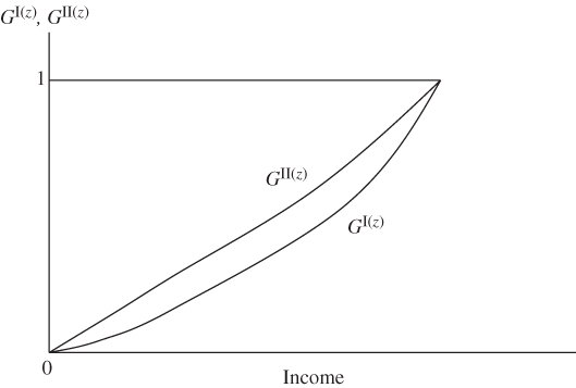
Figure 3.2 First order stochastic dominance.
Next, assume that poverty assessment is performed with the poverty gap ratio. Foster and Shorrocks (1988) demonstrated that dominance of GII over GI with respect to the poverty gap ratio is equivalent to the requirement that GI second order stochastic dominates GII. Graphically, at any income, the area under the curve of GI never exceeds the corresponding area under the curve of GII (see Figure 3.3). Equivalently, we say that areawise dominance of the graph of GII over that of GI has to hold.16 Second order stochastic dominance of GI over GII is also equivalent to the condition that GI is not generalized Lorenz inferior to GII; the generalized Lorenz curve of GI does not lie below that of GII.

Figure 3.3 Second order stochastic dominance.
From Figure 3.3, it follows clearly that up to any level of income z, the area under the curve of GII is not lower than the corresponding area under the curve of GI. Hence, second order stochastic dominance of GI over GII holds. From the figures, it also follows that first order dominance implies the second order dominance, but the converse is not true. In other words, first order dominance is a sufficient but not a necessary condition for second order dominance. This shows that as we move from the first order condition to the next higher order condition, the ranking power becomes thinner. The reason behind this is that in the case of the latter, we need areawise dominance starting from the initial income level. As a result, one or more intersections between the curves of the distribution functions are permissible; the only restriction we need to follow is that area under GI does not exceed the area under GII at any income level. But for the first order dominance to hold, we need pointwise dominance, and as a result, no intersection between the curves is allowed.17 (Formal treatments of stochastic dominance relations are available in Hadar and Russell, 1969; Whitmore, 1970; Levy, 2006; Shaked and Shanthikumar, 2006 and Chakravarty, 2013.)
3.7.2 Multidimensional Orderings
Duclos et al. (2006a) and Bourguignon and Chakravarty (2009) developed conditions for poverty ranking of alternative multivariate distributions of achievements. Recall that each column of an achievement matrix represents the marginal distribution of a particular dimension (see Section 3.3). Ranking of dimension-wise marginal distributions in two distribution matrices ignores association among dimensions, an important characteristic in multidimensional well-being analysis. Duclos et al. (2006a) compared child poverty in two dimensions between Madagascar and Cameroon and noted statistically significant dominations for each of the two marginal distributions. Nevertheless, no unambiguous domination was observed for the joint distributions. This clearly confirms that simple comparisons of marginal distributions across social matrices do not give us a comprehensive picture of the issue. In consequence, the ranking analysis should explicitly involve the matrices as a whole.
Gravel and Mukhopadhyay (2010) employed generalizations, to three dimensions or more, of the Atkinson and Bourguignon (1982) first and second order dominance criteria to provide a normative assessment of growth in India over the 1987–2002 period. The four dimensions, considered in their analysis, are real consumption (measured at the individual level), literacy rate, under-5 mortality, and violent crime rates (all measured at the district levels). Their findings indicate that India was better off in 2002 than in 1995 or 1987 by the second order dominance rule. However, if violent crime rates are excluded from the list of dimensions, the dominance was found to be steady over the entire period.18
As we have observed, in a multidimensional setup, identification of the poor is an important ingredient of poverty evaluation. A “poverty frontier,” defined as alternative combinations of all dimensional achievements that produce an overall achievement, which equals an aggregate or comprehensive poverty line, is taken as the identification indicator. The comprehensive poverty line is assumed to render a subsistence standard of living. It is gathered by aggregating the poverty cutoff limits across all dimensions, where the underlying aggregation function is the same as that employed to deduce an overall achievement. Subsequently, a person is identified as poor if his achievements in all the dimensions generate a lower level of aggregated achievement than the comprehensive poverty line. The frontier, thus, separates the poor from the nonpoor.
Given a particular poverty frontier, of two social distributions ![]() , X is said to be poverty dominated by Y in the Duclos–Sahn–Younger sense if and only if
, X is said to be poverty dominated by Y in the Duclos–Sahn–Younger sense if and only if ![]() for all
for all ![]() . We denote this relation by
. We denote this relation by ![]() .
.
Duclos et al. (2006a) developed stochastic dominance-based poverty ordering results for achievement matrices with two dimensions of well-being. To analyze these results, let us denote the achievements in the two dimensions by x1 and x2, respectively, assuming that the dimensions are substitutes. Let ![]() stand for the joint distribution of x1 and x2. Formally,
stand for the joint distribution of x1 and x2. Formally, ![]() . The joint distribution shows simultaneously the proportion of population enjoying achievement levels x1 and x2 not exceeding q1 and q2, respectively. The marginal distribution of xi is expressed by
. The joint distribution shows simultaneously the proportion of population enjoying achievement levels x1 and x2 not exceeding q1 and q2, respectively. The marginal distribution of xi is expressed by ![]() , where
, where ![]() .
.
Duclos et al. (2006a) showed that under substitutability assumption between the dimensions, if ![]() for all
for all ![]() , then
, then ![]() holds for all two dimensional subgroup-decomposable poverty indices that are nonincreasing in dimensional achievements, where
holds for all two dimensional subgroup-decomposable poverty indices that are nonincreasing in dimensional achievements, where ![]() is the joint cumulative distribution function for
is the joint cumulative distribution function for ![]() . The inequality
. The inequality ![]() means that the joint cumulative distribution function of Y does not lie below that of X cumulated up to
means that the joint cumulative distribution function of Y does not lie below that of X cumulated up to ![]() . The underlying class of indices includes the family of indices suggested by Chakravarty et al. (1998), Tsui (2002), Chakravarty et al. (2008), Alkire and Foster (2011a,b) and some members of the family proposed by Bourguignon and Chakravarty (2003) (see also Bresson and Duclos, 2015).
. The underlying class of indices includes the family of indices suggested by Chakravarty et al. (1998), Tsui (2002), Chakravarty et al. (2008), Alkire and Foster (2011a,b) and some members of the family proposed by Bourguignon and Chakravarty (2003) (see also Bresson and Duclos, 2015).
The poverty frontier is implicitly defined by a locus ![]() , where the aggregator is continuous and nondecreasing in its arguments. Bidimensional poverty is now defined by the
, where the aggregator is continuous and nondecreasing in its arguments. Bidimensional poverty is now defined by the ![]() combinations for which
combinations for which ![]() , and the poverty domain is given by
, and the poverty domain is given by ![]() .
.
In Figure 3.4, the poverty frontier is represented by the curve A. Since ![]() signifies the proportion of population with achievements simultaneously less than or equal to q1 in dimension 1 and q2 in dimension 2, under
signifies the proportion of population with achievements simultaneously less than or equal to q1 in dimension 1 and q2 in dimension 2, under ![]() , the inequality
, the inequality ![]() is an intersection type condition. If
is an intersection type condition. If ![]() is not lower than
is not lower than ![]() for all rectangles B, C, and so on that fit within
for all rectangles B, C, and so on that fit within ![]() , then the dominance
, then the dominance ![]() follows. Hence, an attractive feature of this dominance condition is that we only need to check intersection-type conditions.
follows. Hence, an attractive feature of this dominance condition is that we only need to check intersection-type conditions.

Figure 3.4 Bidimensional poverty ordering.
Bourguignon and Chakravarty (2009) developed related first order bidimensional dominance conditions involving the joint distributions and the marginal distributions. In their highly innovative contribution, Aaberge and Brandolini (2015) provided an excellent overview of the Bourguignon–Chakravarty orderings. Here we furnish a sketch of their main findings. They demonstrated that poverty dominance for two bidimensional achievement matrices for all poverty indices that are strongly focussed, symmetric, subgroup decomposable, population replication invariant, nonincreasing in achievements of the poor, and nondecreasing under a correlation-increasing switch (substitutability) holds if and only if there is unambiguous dominance for each marginal distribution and the intersection area. Graphically, the areas of all intersection rectangles for the dominant matrix should not be less than the corresponding areas of the dominated ones, and the marginal distribution function for each dimension in the dominated matrix cannot lie above that of the dominant one. (See Figure 3.4.)
In a subsequent result, Bourguignon and Chakravarty (2009) retained all the poverty postulates stated earlier except nondecreasingness under a correlation-increasing switch, which has been replaced by nonincreasingness under the switch (complementarity). They then established that necessary and sufficient conditions in such a situation are dominance for each marginal distribution and dominance with respect to joint distribution in union area (see Figure 3.1).
3.8 Dimensions of Well-Being with Ordinal Significance and Multidimensional Poverty
It has already been observed in Chapter 1 that values of ordinally measurable dimensions are only indicators of order. Specific numerical values assigned to represent the ordering are insignificant. Recall that each notion of measurability allows some admissible transformation that can be applied to dimensional achievements so that no loss of information occurs. In other words, the value of a quantifier that relies on dimensional achievements remains unaltered when we transform the achievements by applying some admissible transformations.
We write ![]() for the set of all dimensions of well-being that are measurable on ordinal scale. The corresponding set of dimensional thresholds is denoted by
for the set of all dimensions of well-being that are measurable on ordinal scale. The corresponding set of dimensional thresholds is denoted by ![]() . Let
. Let ![]() (say) be the number of elements in
(say) be the number of elements in ![]() . This is the exogenously given number of dimensions of well-being with ordinal significance. For any
. This is the exogenously given number of dimensions of well-being with ordinal significance. For any ![]() , let
, let ![]() stand for the set of all
stand for the set of all ![]() dimensional matrices of achievements in different dimensions. The set of all such matrices is given by
dimensional matrices of achievements in different dimensions. The set of all such matrices is given by ![]() , where
, where ![]() . A multidimensional poverty index
. A multidimensional poverty index ![]() in an ordinal framework is a real-valued function defined on
in an ordinal framework is a real-valued function defined on ![]() . More precisely,
. More precisely, ![]() . In other words, for any
. In other words, for any ![]() ,
, ![]() ,
, ![]() is the level of poverty that exists in the society given that the dimensions of well-being are ordinally significant.
is the level of poverty that exists in the society given that the dimensions of well-being are ordinally significant.
The information invariance assumption can now be analytically stated as follows. For any ![]() ,
, ![]() , we say that
, we say that ![]() is derived from
is derived from ![]() using a permissible transformation if for each
using a permissible transformation if for each ![]() , there exists an increasing transformation
, there exists an increasing transformation ![]() such that
such that ![]() and
and ![]() , where
, where ![]() is the threshold point of
is the threshold point of ![]() . In other words,
. In other words, ![]() is the jth coordinate of the vector
is the jth coordinate of the vector ![]() . We do not assume that the transformations
. We do not assume that the transformations ![]() are the same across dimensions. The ordinality property, which we also refer to as ordinal information invariance assumption, then requires that
are the same across dimensions. The ordinality property, which we also refer to as ordinal information invariance assumption, then requires that ![]() .
.
Essentials to the construction of a multidimensional poverty index when dimensions have ordinal significance are deprivation counts of the individuals. The deprivation count of a person relies on a dichotomous or binary variable. A variable may be binary by definition: for instance, whether a person is a citizen of a given country or not. But often it may be useful to derive binary variables from nonbinary variables. For instance, weights of individuals in a region can assume more than two values. However, we can segregate these persons into two subgroups: those who weigh less than 60 kilograms and those weighing at least 60 kilograms. This is a simple creation of a binary variable from a nonbinary variable.
In the current context, we dichotomize each ordinal dimension by comparing a person's achievement in the dimension with its norm, the threshold limit. If somebody's achievement in the dimension is associated with a category that has a lower rank than the category to which the threshold limit corresponds, then he is deprived in the dimension, given that the categories are ranked in increasing order of preferences, that is, from the worst to the best. Otherwise, the person is nondeprived in the dimension. We assign the values 1 and 0, respectively, to indicate deprivation and nondeprivation of a person in a dimension possessing ordinal characteristic.
For any ![]() ,
, ![]() ,
, ![]() , let
, let ![]() , (
, (![]() , for short) denote person i's deprivation metric for
, for short) denote person i's deprivation metric for ![]() . More precisely,
. More precisely, ![]() if person i is deprived in the ordinal dimension j and
if person i is deprived in the ordinal dimension j and ![]() , otherwise. Then the deprivation profile of the person associated with the ordinal dimensions in the set
, otherwise. Then the deprivation profile of the person associated with the ordinal dimensions in the set ![]() is
is ![]() , where
, where ![]() . Then the deprivation count of person i in ordinal dimensions is
. Then the deprivation count of person i in ordinal dimensions is ![]() . Clearly,
. Clearly, ![]() is a nonnegative integer bounded between 0 and k. The lower bound is achieved if the person is not deprived in ordinal dimensions, and the upper bound is attained when he has deprivations in all the dimensions. The distribution of deprivation counts in ordinally significant dimensions across individuals in the society is given by
is a nonnegative integer bounded between 0 and k. The lower bound is achieved if the person is not deprived in ordinal dimensions, and the upper bound is attained when he has deprivations in all the dimensions. The distribution of deprivation counts in ordinally significant dimensions across individuals in the society is given by ![]() . Person i is regarded as union poor in this ordinal framework if
. Person i is regarded as union poor in this ordinal framework if ![]() . However, the intersection rule treats the person as poor if
. However, the intersection rule treats the person as poor if ![]() . (See Cappellari and Jenkins, 2007, for a discussion.)
. (See Cappellari and Jenkins, 2007, for a discussion.)
As an illustrative example, assume that in a four-person society, there are only two dimensions of well-being: self-reported health status and literacy grade. In the dimension self-reported health condition, we assign the numbers 1, 4, 9, 16, 25, and 36 to the six health categories “very poor,” “poor,” “fair,” “good,” “very good,” and “excellent” to indicate that a higher number is assigned to a better category.19 Suppose that the category “good” represents the threshold category, and it is identified with the number 16. Assume that out of four individuals in the society, the first and third individuals have health conditions characterized by the categories “very poor,” “poor” so that they suffer from health deprivation. The heath conditions of the second and fourth persons belong to the categories “excellent” and “good,” respectively. Consequently, they are not health-deprived. For the second dimension, literacy level, the numbers assigned to the categories “illiteracy,” “knowledge just to read and write,” “elementary school graduation,” “high school graduation,” and “college graduation” are respectively 0, 0.1, 0.2, 0.3, and 0.4. The threshold limit of this dimension is 0.1, that is, the ability just to read and write only is taken as the threshold education category. Assume that the levels of education of the four persons are respectively “illiteracy,” “high school graduation,” “knowledge just to read and write,” and “college graduation.” Then the threshold education level is identified by the number 0.1. If we denote the two dimensions by 1 and 2, respectively, and the distribution matrix by ![]() , then
, then  and
and ![]() .
.
In ![]() , while person 1 is deprived in both the dimensions, person 3 is deprived only in dimension 1. On the other hand, none of persons 2 and 4 is deprived in any dimension. Consequently, the deprivation profiles of these four persons are given, respectively, by
, while person 1 is deprived in both the dimensions, person 3 is deprived only in dimension 1. On the other hand, none of persons 2 and 4 is deprived in any dimension. Consequently, the deprivation profiles of these four persons are given, respectively, by ![]() ,
, ![]() ,
, ![]() , and
, and ![]() . This in turn shows that the deprivation counts of the four persons, the numbers of dimensions in which they are deprived are given respectively by 2, 0, 1, and 0.
. This in turn shows that the deprivation counts of the four persons, the numbers of dimensions in which they are deprived are given respectively by 2, 0, 1, and 0.
Now, let us assign the numbers 1, 2, 3, 4, 5, and 6 to the self-reported health categories by taking square roots of the previously assigned numbers. Similarly, we assign the numbers 0.01, 0.04, 0.09, and 0.16 by simply squaring the numbers allotted earlier to the grades of literacy. Formally, we transform the dimensional achievements in these two dimensions by applying the increasing transformations ![]() and
and ![]() , where
, where ![]() is the increasing transformation applied to the achievements in dimension
is the increasing transformation applied to the achievements in dimension ![]() and t denotes a dimensional achievement. The threshold limit vector
and t denotes a dimensional achievement. The threshold limit vector ![]() gets converted into
gets converted into ![]() and the transformed achievement matrix becomes
and the transformed achievement matrix becomes  . It is easy to check that the individual deprivation counts remain unchanged under these ordinal transformations of dimensional achievements.
Hence, union poverty head-count ratio turns out to be ![]() , whereas according to the intersection rule, this ratio becomes
, whereas according to the intersection rule, this ratio becomes ![]() . The ordinal information invariance assumption demands that
. The ordinal information invariance assumption demands that ![]() .
.
It is then easy to check that the values of the union and the intersection head-count ratios are the same for ![]() and
and ![]() , given that the corresponding threshold limit vectors are
, given that the corresponding threshold limit vectors are ![]() and
and ![]() , respectively. In other words, the head-count ratio remains unaltered under allowable transformations in the ordinal framework. In consequence, the head-count ratio measure of multidimensional poverty has an advantage over many other indices of multidimensional poverty indices in the sense of its fulfillment of the ordinality property. This holds irrespective of whether the union, intersection, or the intermediate identification rule is employed to determine the set of poor persons. A second index that fulfils this property is the Alkire and Foster (2011a,b) adjusted head-count ratio. This index satisfies dimensional monotonicity property as well, whereas the head-count ratio is a violator of the postulate.
, respectively. In other words, the head-count ratio remains unaltered under allowable transformations in the ordinal framework. In consequence, the head-count ratio measure of multidimensional poverty has an advantage over many other indices of multidimensional poverty indices in the sense of its fulfillment of the ordinality property. This holds irrespective of whether the union, intersection, or the intermediate identification rule is employed to determine the set of poor persons. A second index that fulfils this property is the Alkire and Foster (2011a,b) adjusted head-count ratio. This index satisfies dimensional monotonicity property as well, whereas the head-count ratio is a violator of the postulate.
3.9 Orderings Based on Deprivations Counts
Chakravarty and Zoli (2012) used an axiomatic framework to derive some integer majorization results that can be easily transformed into deprivation profile ranking structure. These results apply to both ordinal and nonordinal dimensions of well-being. Consequently, the set of dimensions can include pension income, interest income, public goods, environmental conditions, and so on. Given that there are ![]() such dimensions of well-being, denote the functioning score of person
such dimensions of well-being, denote the functioning score of person ![]() by
by ![]() , where
, where ![]() is arbitrary. In other words,
is arbitrary. In other words, ![]() is the number of dimensions in which person i is not deprived. Evidently,
is the number of dimensions in which person i is not deprived. Evidently, ![]() . The lower bound 0 of
. The lower bound 0 of ![]() arises when the person is deprived in all the dimensions. On the other hand, the upper bound
arises when the person is deprived in all the dimensions. On the other hand, the upper bound ![]() is achieved whenever the individual becomes nondeprived in all the dimensions. Let
is achieved whenever the individual becomes nondeprived in all the dimensions. Let ![]() be a profile of functioning scores of the persons in the society. The functioning score distribution
be a profile of functioning scores of the persons in the society. The functioning score distribution ![]() is an element of
is an element of ![]() , the n-fold Cartesian product of
, the n-fold Cartesian product of ![]() . Clearly, the deprivation count
. Clearly, the deprivation count ![]() of person
of person ![]() is given by
is given by ![]() . That is, given any profile
. That is, given any profile ![]() of functioning scores, we can write its deprivation counterpart as
of functioning scores, we can write its deprivation counterpart as ![]() , where 1n is the n-coordinated vector of 1s. It then follows that the profile
, where 1n is the n-coordinated vector of 1s. It then follows that the profile ![]() of deprivation counts is also an element of
of deprivation counts is also an element of ![]() .
.
The nonincreasingly ordered permutation of τ is denoted by ![]() , that is,
, that is, ![]() and
and ![]() . Similarly, we write
. Similarly, we write ![]() for the nondecreasingly ordered permutation of τ, that is,
for the nondecreasingly ordered permutation of τ, that is, ![]() . Similarly ordered permutations of
. Similarly ordered permutations of ![]() are denoted by
are denoted by ![]() and
and ![]() , respectively.
, respectively.
Chakravarty and Zoli (2012) considered distributions of functioning scores across persons and established the equivalence between five dominance conditions. Of particular interest is their demonstration that if one vector of functioning scores generalized Lorenz dominates that of another, then the former is preferred to the latter by the generalized Gini welfare function. The converse is true as well.
As a background material of deprivation count ordering, we now analyze the Chakravarty–Zoli dominance results. Of two profiles of functioning scores ![]() , we say that τ is obtained from
, we say that τ is obtained from ![]() by a favorable composite change if there exists individuals
by a favorable composite change if there exists individuals ![]() such that
such that ![]() and
and ![]() and
and ![]() for all
for all ![]() . In
. In ![]() , person i's functioning score exceeds that of person j by at least 2, and
, person i's functioning score exceeds that of person j by at least 2, and ![]() is transformed into τ by reducing i's functioning score by 1 and increasing that of j by 1. The transformation decreases the variance of the distribution of functioning scores without changing the mean. Consequently, it leads to an improvement in well-being of the society. The restriction
is transformed into τ by reducing i's functioning score by 1 and increasing that of j by 1. The transformation decreases the variance of the distribution of functioning scores without changing the mean. Consequently, it leads to an improvement in well-being of the society. The restriction ![]() ensures that
ensures that ![]() , that is, the relative position of the affected individuals remains the same. (See Chakravarty and D'Ambrosio, 2006 and Chakravarty and Zoli, 2012.)
, that is, the relative position of the affected individuals remains the same. (See Chakravarty and D'Ambrosio, 2006 and Chakravarty and Zoli, 2012.)
We say that τ is obtained from ![]() by a simple increment if for some
by a simple increment if for some ![]() such that
such that ![]() ,
, ![]() and
and ![]() for all
for all ![]() . In other words, we deduce τ is from
. In other words, we deduce τ is from ![]() by increasing person j's functioning score by 1 and keeping all other persons' scores unchanged.
by increasing person j's functioning score by 1 and keeping all other persons' scores unchanged.
Now, consider a functioning evaluation standard ![]() , a nonnegative real-valued function defined on
, a nonnegative real-valued function defined on ![]() . Formally,
. Formally, ![]() . For any
. For any ![]() ,
, ![]() indicates the extent of well-being enjoyed by the individuals in the society corresponding to the distribution τ of functioning scores across the individuals. A standard
indicates the extent of well-being enjoyed by the individuals in the society corresponding to the distribution τ of functioning scores across the individuals. A standard ![]() is said to be increasing if
is said to be increasing if ![]() whenever τ is obtained from
whenever τ is obtained from ![]() by a simple increment. It satisfies the principle of favorable composite change if its value increases under a favorable composite change.
by a simple increment. It satisfies the principle of favorable composite change if its value increases under a favorable composite change.
The following dominance theorem of Chakravarty and Zoli (2012) can now be stated.
In condition (i), decreasingness of the population-size-dependent positive sequence ![]() ensures that the value of generalized Gini functioning evaluation is higher for the profile τ compared to that for the profile
ensures that the value of generalized Gini functioning evaluation is higher for the profile τ compared to that for the profile ![]() (see Weymark, 1981 and Yaari, 1987). According to condition (ii), of two distributions τ and
(see Weymark, 1981 and Yaari, 1987). According to condition (ii), of two distributions τ and ![]() of functioning scores, the former integer generalized Lorenz dominates that of the latter, that is, the generalized Lorenz curve of the former lies nowhere below that of the latter and lies above in at least some places. Condition (iii) says that the profile τ is regarded as socially better than the profile
of functioning scores, the former integer generalized Lorenz dominates that of the latter, that is, the generalized Lorenz curve of the former lies nowhere below that of the latter and lies above in at least some places. Condition (iii) says that the profile τ is regarded as socially better than the profile ![]() by all evaluation standards that are increasing, symmetric, and increasing under favorable composite changes. Conditions (iv) and (v) are self-explanatory. Conditions (ii)–(v) can be regarded as integer counterparts of some well-known majorization results existing in the literature on univariate inequality measurement (see Marshall et al., 2011, p. 14 and p. 87).20
by all evaluation standards that are increasing, symmetric, and increasing under favorable composite changes. Conditions (iv) and (v) are self-explanatory. Conditions (ii)–(v) can be regarded as integer counterparts of some well-known majorization results existing in the literature on univariate inequality measurement (see Marshall et al., 2011, p. 14 and p. 87).20
To illustrate condition (v), consider the functioning score profile ![]() . The profile
. The profile ![]() is deduced from
is deduced from ![]() by increasing person 1's score by 1 accompanied by a rank-preserving favorable composite change involving persons 3 and 4.
by increasing person 1's score by 1 accompanied by a rank-preserving favorable composite change involving persons 3 and 4.
Recall that for all ![]() ,
, ![]() . In consequence, we can easily convert the dominance conditions of vectors of functioning scores into ordering of deprivation count distributions. Note that for any
. In consequence, we can easily convert the dominance conditions of vectors of functioning scores into ordering of deprivation count distributions. Note that for any ![]() ,
, ![]() . Let
. Let ![]() and
and ![]() , respectively, be the deprivation counterparts of the profiles τ and
, respectively, be the deprivation counterparts of the profiles τ and ![]() of functioning scores. If
of functioning scores. If ![]() is obtained from
is obtained from ![]() by a simple increment, an increment in functioning score of a person, we can equivalently say that
by a simple increment, an increment in functioning score of a person, we can equivalently say that ![]() is deduced from
is deduced from ![]() by an increment in his deprivation count. Similarly, if
by an increment in his deprivation count. Similarly, if ![]() is deduced from
is deduced from ![]() by a favorable composite change affecting functioning scores of two individuals, we can as well say that
by a favorable composite change affecting functioning scores of two individuals, we can as well say that ![]() is derived from ξ by an unfavorable composite change that affects deprivation counts of the concerned persons. In the example,
is derived from ξ by an unfavorable composite change that affects deprivation counts of the concerned persons. In the example, ![]() and
and ![]() assume that
assume that ![]() . We can then say that
. We can then say that ![]() is transformed into
is transformed into ![]() by increasing person 1's deprivation count by 1 and an unfavorable composite change entailing persons 4 and 3. (We increase the deprivation count of person 4, the most deprived person in terms of counting, by 1 and reduce that of person 3, who is less deprived than person 4, by 1.)
by increasing person 1's deprivation count by 1 and an unfavorable composite change entailing persons 4 and 3. (We increase the deprivation count of person 4, the most deprived person in terms of counting, by 1 and reduce that of person 3, who is less deprived than person 4, by 1.)
Then condition (ii) of Theorem 3.1 can be restated in terms of dominance between the integer inverse generalized Lorenz curves of the distribution of deprivation counts.21 Formally, this condition becomes (ii)  for all
 ![]() , with > for at least one j. This is the same as the condition that the integer inverse generalized Lorenz curve of
, with > for at least one j. This is the same as the condition that the integer inverse generalized Lorenz curve of ![]() dominates that of
dominates that of ![]() . Condition (i) of the theorem can be rewritten as
. Condition (i) of the theorem can be rewritten as  . In the aggregation, higher weight is assigned higher deprivation counts. This inequality means that the value of the generalized Gini index of deprivation count distribution
 ![]() is higher than that of the distribution
is higher than that of the distribution ![]() .
.
In general, a deprivation count assessment metric ![]() is a nonnegative real-valued function defined on the set of profiles of deprivation count. Formally,
is a nonnegative real-valued function defined on the set of profiles of deprivation count. Formally, ![]() . Such an index provides a social assessment of deprivation counts existing at the individual levels.
. Such an index provides a social assessment of deprivation counts existing at the individual levels.
Conditions (iii)–(v) of the Theorem 3.1 can be modified analogously. Hence, the following theorem, which may be regarded as the deprivation count twin of Theorem 3.1, can now be stated.
The most attractive feature of Theorem 3.2 is equivalence of integer inverse generalized Lorenz ordering with the remaining four conditions each of which has its own merit. Once the dominance condition between integer inverse generalized Lorenz curves of two social matrices hold, we can be sure about their ranking by the generalized Gini deprivation index, where the positive increasing weights assigned to nondecreasingly ordered deprivation counts are arbitrary. Similar remarks hold for other equivalent conditions (see Chakravarty and Zoli, 2012).
Lasso de La Vega (2010) examined dominance conditions to ensure unanimous poverty ranking in a counting framework. These orderings coincide with the integer first and second order stochastic dominance orderings. Theorem 3.2 of the current section is formally equivalent to the integer second order stochastic dominance condition. However, its equivalence with ranking in terms of the generalized Gini index of the count distribution has not been demonstrated rigorously earlier (see also Silber and Yalonetzky, 2014 and Yalonetzky, 2014). Aaberge and Peluso (2011) compared distributions of deprivation counts by employing summary measures of deprivation within the rank-dependent social evaluation framework (Sen, 1974; Yaari, 1987).
3.10 Multidimensional Material Deprivation
Material deprivation can be regarded as a situation of economic condition, which follows as a consequence imposed incapability of an individual to acquire achievements not below cutoff limits in different dimensions related to material living conditions. More precisely, multidimensional material deprivation deals with deprivations in dimensions of well-being regarding material conditions.22 We refer to such a dimension as a material dimension. Consequently, qualitative dimensions such as communing with friends and political participation are excluded from the domain of the material deprivation measurement. As maintained by EU policy, indices of material deprivation are to be consolidated with income-dependent poverty measures and quantifiers of low employment.
Examples of material deprivations in nonmonetary dimensions of well-being considered in the “The European Union Statistics on Income and Living Conditions (EU-SILC)” project are incapability to face unexpected required expenses, inability to bear expenses to have a meal with meat, chicken, fish (or vegetarian protein equivalent) every second day, lacking capacity to afford to pay for a one-week annual holiday from residence, not having a durable good such as color television, washing machine, telephone, or car, and so on.
Bossert, Chakravarty and D'Ambrosio (2013) developed an axiomatic characterization of a multidimensional index of material deprivation that relies on the union mode to the identification of the poor. The suggested index turns out to be a weighted sum of material deprivation counts of the individuals, where the material deprivation count of a person is defined as the number of relevant dimensions from which the person is deprived.23
The framework considered deprivation counts because the dimensions were assumed to be discrete in nature. Consequently, it was not possible to determine deprivation in a dimension in terms of shortfall from its threshold limit, which is also nonquantifiable. For instance, possession of a durable good was taken as the threshold limit of the corresponding dimension, and its nonpossession was regarded as deprivation in the dimension. As a result, it was simply necessary to check whether the person has achievement in the dimension or not. The material deprivation count of a person is deduced by calculating the number of material dimensions in which he is deprived. The model rules out the possibility of using continuous dimensions so that an axiom such as ratio-scale invariance becomes inappropriate.
Since the union poverty rule has been employed, a person becomes materially deprived if his deprivation count in appropriate dimensions is at least 1. As a result, for a person to be materially nondeprived, it is necessary that he is not deprived in any accordant dimension, and in such a case, the person's deprivation count is 0. This does not rule the possibility that he is not multidimensionally poor; he may be deprived in one or more nonmaterial living conditions.
Of the three axioms that were employed in the characterization result, the first, zero normalization is a cardinality property. According to this postulate, the index takes on the value zero whenever in a one-person society, the person is not deprived in any dimension. The second axiom is the factor decomposability postulate introduced by Chakravarty et al. (1998). The third axiom is population subgroup decomposability.
To present the index analytically, we assume that there are ![]() material dimensions of well-being and denote the material deprivation count of person
material dimensions of well-being and denote the material deprivation count of person ![]() by
by ![]() . The superscript m signifies that our concern here is with material deprivation. Clearly,
. The superscript m signifies that our concern here is with material deprivation. Clearly, ![]() is a nonnegative integer bounded between 0 and
is a nonnegative integer bounded between 0 and ![]() , the total number of materialistic dimensions. The lower bound is achieved if the person is not materially deprived and the upper bound is attained when he has deprivations in all the dimensions. The material deprivation profile in an n-person society is denoted by
, the total number of materialistic dimensions. The lower bound is achieved if the person is not materially deprived and the upper bound is attained when he has deprivations in all the dimensions. The material deprivation profile in an n-person society is denoted by ![]() . The vector
. The vector ![]() is an element of the set
is an element of the set ![]() , the n-fold Cartesian product of the set
, the n-fold Cartesian product of the set ![]() .
.
The Bossert et al. (2013) material deprivation index is defined as

where ![]() ,
, ![]() are arbitrary,
are arbitrary, ![]() is the set of all persons who are materially deprived in
is the set of all persons who are materially deprived in ![]() , and
, and ![]() is the weight assigned to the jth material dimension. It represents the importance assigned to dimension j in the aggregation. The index in (3.22) satisfies a monotonicity property; if a person who was deprived in a material dimension now becomes nondeprived in it because of, improvement in living conditions, say, then value of Bm reduces. The individuals are treated symmetrically in (3.22) in the sense that if two individuals are deprived in the same set of material dimensions, then their material deprivation counts are the same. If
is the weight assigned to the jth material dimension. It represents the importance assigned to dimension j in the aggregation. The index in (3.22) satisfies a monotonicity property; if a person who was deprived in a material dimension now becomes nondeprived in it because of, improvement in living conditions, say, then value of Bm reduces. The individuals are treated symmetrically in (3.22) in the sense that if two individuals are deprived in the same set of material dimensions, then their material deprivation counts are the same. If ![]() for all material dimensions j, then Bm is simply the head-count ratio of material deprivation, the proportion of persons who are materially deprived.
for all material dimensions j, then Bm is simply the head-count ratio of material deprivation, the proportion of persons who are materially deprived.
Earlier Chakravarty and D'Ambrosio (2006) characterized the following measure of social exclusion, which can be regarded as a material deprivation metric:

where ![]() ,
, ![]() and f is increasing. Increasingness of f guarantees that the value of Cm increases if the material deprivation count of a person goes up.
and f is increasing. Increasingness of f guarantees that the value of Cm increases if the material deprivation count of a person goes up.
A functional form of f under which increasingness of material deprivation index holds is ![]() , where
, where ![]() is a parameter. The resulting functional form of Cm becomes
is a parameter. The resulting functional form of Cm becomes ![]() . The parametric restriction
. The parametric restriction ![]() ensures that
ensures that ![]() is monotonic. (Jayaraj and Subramanian (2010) applied the index Cm to study multidimensional deprivation in India using data from National Family Health Surveys.)
is monotonic. (Jayaraj and Subramanian (2010) applied the index Cm to study multidimensional deprivation in India using data from National Family Health Surveys.)
An example of a nonadditive material deprivation index is the generalized Gini index defined by ![]() , where the decreasing, positive sequence
, where the decreasing, positive sequence ![]() depends on the population size
depends on the population size ![]() affected by material deprivation, and
affected by material deprivation, and ![]() is the nonincreasingly ordered permutation of
is the nonincreasingly ordered permutation of ![]() , that is,
, that is, ![]() for all
for all ![]() . Assignment of higher weights to higher material deprivation counts in the generalized Gini index reflects the idea that the deprivation index has an increasing marginal.
. Assignment of higher weights to higher material deprivation counts in the generalized Gini index reflects the idea that the deprivation index has an increasing marginal.
To state the increasing marginal material deprivation property formally, consider the change in material deprivation when person i's materialistic deprivation count increases by 1, where ![]() is arbitrary. Analytically, given
is arbitrary. Analytically, given ![]() , this change is given by
, this change is given by ![]() . Since this difference in the deprivation index arises from a marginal increase in person i's deprivation count in materialistic dimensions, we refer to it as marginal material deprivation. Of two arbitrary persons
. Since this difference in the deprivation index arises from a marginal increase in person i's deprivation count in materialistic dimensions, we refer to it as marginal material deprivation. Of two arbitrary persons ![]() , if the material deprivation of each of them increases by 1, where i has higher number of deprivation count than j in the relevant dimensions, then increasingness of marginal material deprivation means that
, if the material deprivation of each of them increases by 1, where i has higher number of deprivation count than j in the relevant dimensions, then increasingness of marginal material deprivation means that  , which we can rewrite as
  . Under additivity of Fm, that is, if it is of the type
 ![]() , where
, where ![]() , then increasingness of marginal evaluation requires the satisfaction of the inequality
, then increasingness of marginal evaluation requires the satisfaction of the inequality ![]() , where
, where ![]() and
and ![]() are arbitrary.
are arbitrary.
We can now formally say that the index Fm satisfies the increasing marginal material deprivation property if for all ![]() ,
,  , where
 ![]() .
.
We note that the material deprivation count of each of the two persons i and j increases by 1 and j has lower count than i. Then increasingness of material deprivation demands that the increase in society material deprivation resulting from worsening in person i's deprivation count in material dimensions is higher than the corresponding increase that arises as a result of similar aggravation in person j's position. In other words, higher weight is assigned to increase in social assessment of material deprivations as the number of materially deprived dimensions of a person increases.24 Recall that this has been done in the generalized Gini material deprivation index ![]() . For the additive index
. For the additive index ![]() , the parametric restriction
, the parametric restriction ![]() is necessary and sufficient for fulfillment of this postulate.25
is necessary and sufficient for fulfillment of this postulate.25
3.11 Concluding Remarks
Several methodologies have been proposed in the literature for the evaluation of poverty from multidimensional standpoints. Each of them has its own objectives and represents a particular mode of assessing poverty using specific means. None of them is designed to overthrow one or more of the others.
In the dashboard mechanism, valuation of poverty is carried out in a primitive framework; the dashboard comprises dimension-by-dimension poverty figures. In the axiomatic approach to the evaluation of multidimensional poverty, a set of desirable postulates for alternative poverty indices is proposed at the outset. Each of these indices or quantifiers is a summary measure of the levels of deprivations arising from insufficiency of achievements in different dimensions of well-being. Broadly speaking, the job then becomes scrutiny of a measure with respect to gratification of one or more of these desiderata. A related issue is to order two or more social matrices, which describe different individuals' positions in terms of their achievements in given dimensions of well-being, indicating society's preference for lower poverty. Several notions of ordering depend on a cumulative joint distribution function, a statistical concept, of a social matrix. Further, it also often becomes necessary to enquire whether poverty ranking by cumulative distribution functions agrees with that produced by axiomatic indices. Consequently, sometimes the ordering process may be interpreted as a mixture of axiomatic and statistical designs, where the latter incorporates many tools that can be invoked for the purpose of poverty evaluation. A second example of a statistical technique employed within the axiomatic framework is the correlation between dimensional achievements that judges interdimensional association.
Additional examples of statistical techniques include principle component analysis; factor analysis (see Chapter1); multiple correspondence analysis used to reveal veiled structures in a given data set; cluster analysis, concerned with grouping of individuals bearing similarity with respect to multidimensional deprivations and structural equations models that are capable of intimating relationships between latent and observed variables.26
Another well-accepted process that exists in the literature is the fuzzy set approach that arises when information concerning the identification of the poor is incomplete (see Chapter 4). Multidimensional poverty analysis sometimes also makes use of information-theory-based technique that relies on information function and related entropies. (See Maasoumi and Lugo, 2008; Roelen et al., 2009; Alkire et al., 2015; Chakravarty and Lugo, 2016 and Section 3.5 of this chapter.) An alternative mention worthy technique employed in this context is the distance function that looks at the distance between achievements of an individual and a yardstick vector (see, e.g., Anderson et al., 2008 and Ramos, 2008). In the Venn diagram method, joint distributions of deprivations of the individuals are presented diagrammatically when the number of dimensions does not exceed 3 (see Alkire et al., 2015).27
References
- Aaberge, R. and A. Brandolini. 2015. Multidimensional Poverty and Inequality. In A.B. Atkinson and F. Bourguignon (eds.) Handbook of Income Distribution, Vol. 2A. Amsterdam: North-Holland, 141–216.
- Aaberge, R. and E. Peluso. 2011. A Counting Approach for Measuring Multidimensional Deprivation. University of Verona, Department of Economia, WP No. 7.
- Abbe, A. 2006. Empirical Analysis of Relative Deprivation and Poverty in Japan. Tokyo, National Institute of Population and Social Security Research.
- Aboudi, R. and D. Thon. 2006. Refinements of Muirhead's Lemma and Income Inequality. Mathematical Social Sciences 51: 201–216.
- Adler, M.D. and M. Fleurbaey (eds.) 2016. Oxford Handbook of Well-Being and Public Policy. New York: Oxford University Press.
- Akerlof, G. 1997. A Model of Social Distance and Social Decisions. Econometrica 65: 1005–1028.
- Alkire, S., M. Apablaza, and E. Jung. 2014. Multidimensional Poverty Measurement for EU-SILC Countries. Research in Progress Series 36c: OPHI.
- Alkire, S. and J.E. Foster. 2011a. Counting and Multidimensional Poverty Measurement. Journal of Public Economics 95: 476–487.
- Alkire S. and J.E. Foster. 2011b. Understandings and Misunderstandings of Multidimensional Poverty Measurement. Journal of Economic Inequality 9: 289–314.
- Alkire S, J.E. Foster, and M. Santos. 2011. Where Did Identification Go? Journal of Economic Inequality 9: 501–505.
- Alkire, S., J.E. Foster, S. Seth, M.E. Santos, J.M. Roche, and P. Ballon. 2015. Multidimensional Poverty Measurement and Analysis. Oxford: Oxford University Press.
- Alkire, S. and J.M. Roche. 2012. Beyond Headcount: Measures that Reflect the Breadth and Components of Child Poverty. In A. Minujin and S. Nandy (eds.), 103–134.
- Alkire, S. and S. Seth. 2008. Determining BPL Status: Some Methodological Improvements. Indian Journal of Human Development 2: 407–424.
- Alkire, S. and S. Seth. 2013a. Identifying the BPL Households. Economic and Political Weekly 48: 49–67.
- Alkire, S. and S. Seth. 2013b. Selecting a Targeting Method to Identify BPL Households in India. Social Indicators Research 112: 417–446.
- Alkire, S. and S. Seth. 2015. Multidimensional Poverty Reduction in India Between 1999-2006: Where and How? World Development 72: 93–108.
- Altimir, O. 1979. La Dimensión de la Pobreza en América Latina. Cuadernos de la Cepal No. 27, Naciones Unidas, Santiago de Chile.
- Anaka, M. and M. Kobus. 2012. Multidimensional Poverty Analysis in Polish Gminas. Ekonomista 112: 101–117.
- Anand, S. 1983. Inequality and Poverty in Malaysia: Measurement and Decomposition. New York: Oxford University Press.
- Anand, S. 1997. Aspects of Poverty in Malaysia. Review of Income and Wealth 23: 1–16.
- Anderson, G., 2008. The Empirical Assessment of Multidimensional Welfare, Inequality and Poverty: Sample Weighted Multivariate Generalizations of the Kolomogorov-Smirnov Two Sample Test for Stochastic Dominance. Journal of Economic Inequality 6: 73–87.
- Anderson, G., I. Crawford, and A. Leicester. 2008. Efficiency Analysis and the Lower Convex Hull Approach. In N. Kakwani and J. Silber (eds.), 191–196.
- Anderson, E. and L. Esposito. 2014. On the Joint Evaluation of Absolute and Relative Deprivation. Journal of Economic Inequality 12: 411–428.
- Anderson, G. and K. Hachem. 2013. Institutions and Economic Outcomes: A Dominance-Based Analysis. Econometric Reviews 32: 164–182.
- Angulo Salazar, R.C., B.Y. Diaz, and R. Pardo Pinzón. 2013. A Counting Multidimensional Poverty Index in Public Policy Context: The Case of Colombia. Working Paper 62: OPHI.
- Apablaza, M. and G. Yalonetzky. 2011. Measuring the Dynamics of Multiple Deprivations among Children: The Cases of Andhra Pradesh, Ethiopia, Peru and Vietnam: OPHI.
- Asselin, L.M. 2009. Analysis of Multidimensional Poverty: Theory and Case Studies. Dordrecht: Springer.
- Asselin, L.M. and V.T. Anh. 2008. Multidimensional Poverty and Multiple Correspondence Analysis. In N. Kakwani and J. Silber (eds.), 80–103.
- Atkinson, A.B.. 1987. On the Measurement of Poverty. Econometrica 55: 749–764.
- Atkinson, A.B. 1998. Social Exclusion, Poverty and Unemployment. CASE/4. Centre for Analysis of Social Exclusion. London School of Economics: 1–20.
- Atkinson, A.B. 2003. Multidimensional Deprivation: Contrasting Social Welfare and Counting Approaches. Journal of Economic Inequality 1: 51–65.
- Atkinson, A.B. 2007. Measuring Top Incomes: Methodological Issues. In A.B. Atkinson and T. Piketty (eds.) Top Incomes over the Twentieth Century. Oxford: Oxford University Press, 18–42.
- Atkinson, A.B. and F. Bourguignon. 1982. The Comparison of Multidimensioned Distributions of Economic Status. Review of Economic Studies 49: 183–201.
- Atkinson, A.B. and F. Bourguignon. 2001. Poverty and Inclusion from a World Perspective. In J.E. Stiglitz and P.A. Muet (eds.) Governance, Equity and Global Markets. New York: Oxford University Press.
- Atkinson, A.B. and F. Bourguignon (eds.). 2015. Handbook of Income Distribution, Vol. 2A. Amsterdam: North-Holland.
- Atkinson, A.B., B. Cantillon, E. Marlier, and B. Nolan. 2002. Social Indicators: The EU and Social Inclusion. Oxford: Oxford University Press.
- Atkinson, A.B., A.-C. Guio, and E. Marlier (eds) (2017) Monitoring Social Inclusion in Europe. Luxembourg: Publications office of the European Union.
- Azevedo, V. and M. Robles. 2013. Multidimensional Targeting: Identifying Beneficiaries of Conditional Cash Transfer Program. Social Indicators Research 112: 447–475.
- Ballon, P. and J.-Y. Duclos. 2015. Multidimensional Poverty in Sudan and South Sudan. Working Paper 93: OPHI.
- Ballon, P. and J. Krishnakumar. 2011. Measuring Capability Poverty: A Multidimensional Model-Based Index. In P. Ballon Model-Based Multidimensional Poverty Indices: Theoretical Construction and Statistical Properties. Doctoral Dissertation: University of Geneva.
- Batana, Y.M. 2013. Multidimensional Measurement of Poverty among Women in Sub-Saharan Africa. Social Indicators Research 112: 337–362.
- Batana, Y.M. and J.-Y. Duclos. 2010. Multidimensional Poverty among West African Children: Testing for Robust Poverty Comparisons. In J. Cockburn and J. Kabubo-Mariara (eds.) Child Welfare in Developing Countries. New York: Springer, 95–122.
- Batana, Y.M. and J.-Y. Duclos. 2011. Comparing Multidimensional Poverty with Qualitative Indicators of Well-Being. In J. Deutsch and J. Silber (eds.) The Measurement of Individual Well-Being and Group Inequalities: Essays in Memory of Z.M. Berrebi. London: Routledge, 280–297.
- Battison, D., G. Cruces, L.F. Lopez-Calva, M.A. Lugo, and M.E. Santos. 2013. Income and Beyond: Multidimensional Poverty in Six Latin American Countries. Social Indicators Research 112: 291–314.
- Bauman, K. 1998. Direct Measures of Poverty as Indicators for Economic Need: Evidence from the Survey of Income and Program Participation. Population Division Working Paper 30. US Census Bureau.
- Bauman, K. 1999. Extend Measures of Well-being: Meeting Basic Needs. Households Economic Studies. US Department of Commerce.
- Bedi, T., A. Coudouel, and A. Smile (eds.) 2007. More Than a Pretty Picture: Using Poverty Maps to Design Better Policies and Interventions. Washington, DC: World Bank.
- Bellani, L. 2013. Multidimensional Indices of Deprivation: The Introduction of Reference Groups Weights. Journal of Economic Inequality 11: 495–516.
- Bennett, C.J. and S. Mitra. 2013. Multidimensional Poverty: Measurement, Estimation and Inference. Econometric Reviews 32: 57–83.
- Bérenger, V. 2016. Measuring Multidimensional Poverty in Three South Asian Countries Using Ordinal Variables. In J. Silber and G. Wan (eds.), 149–214.
- Bérenger, V. and F. Bresson (eds.) 2013a. Monetary Poverty and Social Exclusion Around the Mediterranean Sea. New York: Springer.
- Bérenger, V. and F. Bresson. 2013b. Axiomatic and Robust Multidimensional Poverty Measurements in Five Southern Mediterranean Countries. In V. Bérenger and F. Bresson (eds.), 3–42.
- Bérenger, V., F. Bresson, P. Makdissi, and M. Yazbeck. 2013a. Regional and Sectoral Distribution of Poverty in Lebanon, 2004. In V. Bérenger and F. Bresson (eds.), 109–141.
- Bérenger, V., J. Deutsch, and J. Silber. 2013b. Durable Goods, Access to Services and the Derivation of an Asset Index. Economic Modeling 35: 881–891.
- Berrebi, Z.M. and J. Silber. 1985. Income Inequality Indices and Deprivation: A Generalisation. Quarterly Journal of Economics 100: 807–810.
- Birdsall, N. 2011. Comment on Multidimensional Indices. Journal of Economic Inequality 9: 489–491.
- Blackorby C. and D. Donaldson. 1980. Ethical Indices for the Measurement of Poverty. Econometrica 58: 1053–1060.
- Boarini, R. and M.M. d'Ercole. 2006. Measures of Material Deprivation in OECD Countries. OECD Social, Employment and Migration Working Paper 37.
- Boltvinik, J. 1992. El Metodo de Medición Integrada dela Pobreza: Una propuesta para su desarrollo. Comercio Exterior 42: 354–365.
- Boltvinik, J. 2012. Medición Multidimensional de la Pobreza. América Latina, de precursora a rezagada. La experiencia contrastante de México: una guía para la región?. Paper presented at the Seminario International Multidimencionalidad di la pobreza, ‘Alcances para su definición y evaluación en América Latina y el Caribe’. Universidad de Chile 22–23 November.
- Booth, C. 1894. The Aged Poor: Condition. London: Macmillan.
- Booth, C. 1903. Life and Labor of the People in London. London: Macmillan.
- Booysen, F., R. Servass Van Derberg, M. Von Maltitz, and G. Du Rand. 2008. Using an Asset Index to Assess Trends in Poverty in Seven Sub-Saharan African Countries. World Development 36: 1113–1130.
- Bossert, W., S.R. Chakravarty, and C. D'Ambrosio. 2013. Multidimensional Poverty and Material Deprivation. Review of Income and Wealth 59: 29–43.
- Bossert, W. and C. D'Ambrosio. 2007. Dynamic Measures of Individual Deprivation. Social Choice and Welfare 28: 77–88.
- Bossert, W. and M. Fleurbaey. 2002. Equitable Insurance Premium Schemes. Social Choice and Welfare 19: 113–125.
- Bourguignon, F. and S.R. Chakravarty. 1999. A Family of Multidimensional Poverty Measures. In D.J. Slottje (ed.) Advances in Econometrics, Income Distribution and Scientific Methodology: Essays in Honor of C. Dagum. Heidelberg: Physica-Verlag, 331–342.
- Bourguignon, F. and S.R. Chakravarty. 2003. The Measurement of Multidimensional Poverty. Journal of Economic Inequality, 1, 25–49.
- Bourguignon, F. and S.R. Chakravarty. 2009. Multidimensional Poverty Orderings: Theory and Applications. In K. Basu and R. Kanbur (eds.) Arguments for a Better World: Essays in Honor of Amartya Sen, Volume 1: Ethics, Welfare and Measurement. Oxford: Oxford University Press, 337–361.
- Bowley, A.L. and A.R. Burnett-Hurst. 1915. Livelihood and Poverty: A Study in the Economic and Social Conditions of Working Class Households in Northampton, Warrington, Stanley, Reading (and Bolton). London: King.
- Boyden, J. and M. Bourdillon. 2012. Childhood Poverty: Multidisciplinary Approaches. Basingstoke: Palgrave Macmillan.
- Bradshaw, J. and N. Finch. 2003. Overlaps in Dimensions of Poverty. Journal of Social Policy 32: 513–525.
- Bresson, F. 2009. Multidimensional Poverty Measurement without the Strong Focus Axiom. Université de Nice Sophia Antipolis.
- Bresson, F. and J.-Y. Duclos. 2015. Intertemporal Poverty Comparisons. Social Choice and Welfare 44: 567–616.
- Brzezinski, M. 2010. Income Affluence in Poland. Social Indicators Research 99: 285–299.
- Callan, T., B. Nolan, and C.T. Whelan. 1993. Resources Deprivation and the Measurement of Poverty. Journal of Social Policy 22: 141–172.
- Callander, E.J., D.J. Schofield, and R.N. Shrestha. 2012a. Multiple Disadvantages among Older Citizens: What a Multidimensional Measure of Poverty Can Show? Journal of Aging and Social Policy 24: 368–383.
- Callander, E.J., D.J. Schofield, and R.N. Shrestha. 2012b. Towards a Holistic Understanding of Poverty: A New Multidimensional Measure of Poverty for Australia. Health and Sociology Review 21: 141–155.
- Cappellari, L. and S.P. Jenkins. 2007. Summarizing Multiple Deprivation Indicators. In: S.P. Jenkins and J. Micklewright (ed.) Inequality and Poverty Re-Examined. Oxford: Oxford University Press, 166–184.
- Chakravarty, S.R. 1983. A New Index of Poverty. Mathematical Social Sciences 6: 307–313.
- Chakravarty, S.R. 1990. Ethical Social Index Numbers. New York: Springer.
- Chakravarty, S.R. 2009. Inequality, Polarization and Poverty: Advances in Distributional Analysis, New York: Springer.
- Chakravarty, S.R. 2013. An Outline of Financial Economics. New York: Anthem Press.
- Chakravarty, S.R., N. Chattopadhyay, J. Deutsh, Z. Nissanov, and J. Silber. 2016. Reference Groups and the Poverty Line: An Axiomatic Approach with an Empirical Illustration. Research on Economic Inequality 24: 1–27.
- Chakravarty, S.R. and C. D'Ambrosio. 2006. The Measurement of Social Exclusion. Review of Income and Wealth 52: 377–398.
- Chakravarty, S.R. and C. D'Ambrosio. 2013. A Family of Unit Consistent Multidimensional Poverty Indices. In V. Berenger and F. Bresson (eds.), 75–88.
- Chakravarty S.R., J. Deutsch, and J. Silber. 2008. On the Watts Multidimensional Poverty Index and Its Decomposition. World Development 36: 1067–1077.
- Chakravarty, S.R. and M.A. Lugo. 2016. Multidimensional Indicators of Inequality and Poverty. In M.D. Adler and M. Fleurbaey (eds.), 246–285.
- Chakravarty, S.R. and P. Moyes. 2003. Individual Welfare, Social Deprivation and Income Taxation. Economic Theory 21: 843–869.
- Chakravarty, S.R. and D. Mukherjee. 1999. Measures of Deprivation and Their Meaning in Terms of Social Satisfaction. Theory and Decision 47: 89–100.
- Chakravarty, S.R., D. Mukherjee, and R. Ranade. 1998. On the Family of Subgroup and Factor Decomposable Measures of Multidimensional Poverty. Research on Economic Inequality 8: 175–194.
- Chakravarty, S.R. and J. Silber. 2008. Measuring Multidimensional Poverty: The Axiomatic Approach. In N. Kakwani and J. Silber (eds.), 192–209.
- Chakravarty, S.R. and C. Zoli. 2012. Stochastic Dominance Relations for Integer Variables. Journal of Economic Theory 147: 1331–1341.
- Chen, S. and M. Ravallion. 2001. How did the World's Poorest Fare in the 1990s? Review of Income and Wealth 47: 283–300.
- Chen, S. and M. Ravallion. 2013. More Relatively-Poor People in a Less Absolutely-Poor World. Review of Income and Wealth 59: 1–28.
- Clark, S., R. Hemming, and D. Ulph. 1981. On Indices for the Measurement of Poverty. Economic Journal 91: 515–526.
- Coady, D., M. Grosh, and J. Hoddinot. 2004. Targeting of Transfers in Developing Countries: Review of Lessons and Experience. Washington, DC: World Bank.
- Cohen, A. 2010. The Multidimensional Poverty Assessment Tool: A New Framework for Measuring Rural Poverty. Development in Practice 20: 887–897.
- Cohen, A. and M. Saisana. 2014. Quantifying the Qualitative: Eliciting Expert Input to Develop the Multidimensional Poverty Assessment Tool. Journal of Development Studies 50: 35–50.
- Commission on Growth and Development. 2008. The Growth Report: Strategies for Sustained Growth and Inclusive Development. Washington, DC: World Bank.
- Cowell, F.A. 2016. Inequality and Poverty Measures. In M.D. Adler and M. Fleurbaey (eds.), 82–125.
- D'Ambrosio, C., J. Deutsch, and J. Silber. 2011. Multidimensional Approaches to Poverty Measurement: An Empirical Analysis of Poverty in Belgium, France, Germany Italy and Spain, Based on European Panel. Applied Economics 43: 951–961.
- Datt, G. and M. Ravallion. 1992. Growth and Redistribution Components of Change in Poverty Measures: A Decomposition with Applications to Brazil and India in the 1980s. Journal of Development Economics 38: 275–295.
- Davidson, R. 2008. Stochastic Dominance. In S.N. Durlauf and L.E. Blume (eds.) The New Palgrave Dictionary of Economics, Second Edition. London: Palgrave Macmillan.
- Davidson, R. and J.E. Duclos. 2000. Statistical Inference for Stochastic Dominance and for the Measurement of Poverty and Inequality. Econometrica 68: 1435–1464.
- Davidson, R. and J.E. Duclos. 2013. Testing for Restricted Stochastic Dominance. Econometric Reviews 32: 84–125.
- Davies, R. 1997. Beyond Wealth Ranking: The Democratic Definition and the Measurement of Poverty. Briefing Note Prepared for the ODI Workshop ‘Indicators of Poverty: Operational Significance’ in London, October.
- Davies, R. and W. Smith. 1998. The Basic Necessities Survey (BNS): The Experience of Action Aid Vietnam. Hanoi: Action Aid.
- Deaton A. 2010. Price Indexes, Inequality, and the Measurement of World Poverty. American Economic Review 100: 5–34.
- Decancq, K., M. Fleurbaey, and F. Maniquet. 2015. Multidimensional Poverty Measurement: Shouldn't We Take Preferences into Account? mimeographed, Brussels: CORE.
- Decancq, K., T. Goedemé, K. Van den Bosch, and J. Vanhille. 2013. The Evolution of Poverty in the European Union: Concepts, Measurement and Data. Methodological Paper No. 13/01, ImPRoveE.
- Deineko, V.G., B. Klinz, and G.J. Woeginger. 2009. The Complexity of Computing the Muirhead-Dalton Distance. Mathematical Social Sciences 57: 282–284.
- Deutsch, J., A.-C. Guio, M. Pomati, and J. Silber. 2015. Material Deprivation in Europe: Which Expenditures Are Curtailed First? Social Indicators Research 120: 723–740.
- Deutsch, J. and J. Silber. 2005. Measuring Multidimensional Poverty: An Empirical Comparison of Various Approaches. Review of Income and Wealth 51: 145–174.
- Deutsch, J. and J. Silber. 2008. The Order of Acquisition of Durable Goods and the Measurement of Multidimensional Poverty. In N. Kakwani and J. Silber (eds.), 226–243.
- Deutsch, J., J. Silber, and P. Verme. 2012. On Social Exclusion in Macedonia: Measurement and Determinants. In C. Ruggeri Laderchi and S. Savastano (eds.) Poverty and Exclusion in the Western Balkans: New Directions in Measurement and Policy. New York: Springer.
- Dhongde, S., Y. Li, P.K. Pattanaik, and Y. Xu. 2016. Binary Data, Hierarchy of Attributes, and Multidimensional Deprivation. Journal of Economic Inequality 14: 363–378.
- Di Tommaso, M. 2007. Children Capabilities: A Structural Equation Model for India. Journal of Socio-Economics 36: 436–450.
- Dickerson, A. and G. Popli. 2015. The Many Dimensions of Child Poverty: Evidence from the UK Millennium Cohort Study. Sheffield Economic Research Paper Series no. 2015-09: Institute for Economic Analysis and Decision Making, University of Sheffield.
- Diez, H., M.C. Lasso de la Vega, and A. Urrutia. 2008. Multidimensional Unit- and Subgroup Consistent Inequality and Poverty Measures: Some Characterization Results. Research on Economic Inequality 16: 189–211.
- Donaldson, D. and J.A. Weymark. 1986. Properties of Fixed-Population Poverty Indices. International Economic Review 27: 667–688.
- Drèze, J. and R. Khera. 2010. The BPL Census and a Possible Alternative. Economic and Political Weekly 45: 54–63.
- Drèze, J. and A.K. Sen. 2013. Uncertain Glory:India and Its Contradictions. London: Allen Lane.
- Duclos, J.-Y. and D. Échevin. 2011. Health and Income: A Robust Comparison of Canada and the US. Journal of Health Economics 30: 293–302.
- Duclos, J.-Y., D.E. Sahn, and S.D. Younger. 2006a. Robust Multidimensional Poverty Comparisons. Economic Journal 116: 943–968.
- Duclos, J.-Y., D.E. Sahn, and S.D. Younger. 2006b. Robust Multidimensional Spatial Poverty Comparisons in Ghana, Madagascar, and Uganda. World Bank Economic Review 20: 91–113.
- Duclos, J.-Y., D.E. Sahn, and S.D. Younger. 2007. Robust Multidimensional Poverty Comparisons with Discrete Indicators of Well-Being. In S.P. Jenkins and J. Micklewright (eds.) Inequality and Poverty Re-examined. Oxford: Oxford University Press.
- Duclos, J.-Y., D.E. Sahn, and S.D. Younger. 2008 Using an Ordinal Approach to Multidimensional Poverty Analysis. In N. Kakwani and J. Silber (eds.), 244–261.
- Duclos, J.-Y., D.E. Sahn, and S.D. Younger. 2011. Partial Multidimensional Inequality Orderings. Journal of Public Economics 95: 225–238.
- Duclos, J.-Y. and L. Tiberti. 2016. Multidimensional Poverty Indices: A Critical Assessment. In M.D. Adler and M. Fleurbaey (eds.) The Oxford Handbook of Well-Being and Public Policy. Oxford University Press, 677–708.
- Elbers, C., T. Fuji, P. Lanjouw, B. Özler, and W. Yin 2007. Poverty Alleviation Through Geographic Targeting: How Much Does Disaggregation Help? Journal of Development Economics 71: 355–364.
- Elbers, C., J.O. Lanjouw, and P. Lanjouw. 2002. Micro-Level Estimation of Poverty and Inequality. Econometrica 71: 355–364.
- Erikson, R. 1993. Descriptions of Inequality: The Swedish Approach to Welfare Research. In M. Nussabaum and A.K. Sen (eds.) The Quality of Life. New York: Oxford University Press, 67–83.
- Eurobarameter. 2007. Special Eurobarameter 279/Wave 67/1: Poverty and Exclusion; Report. European Commission.
- Eurostat. 2002. Statistiques Sociales Européennes: Deuxième rapport sur le revenu, la pauvreté et l'exclusion sociale. Luxembourg: Office des publications officielles des communnautés européennes.
- Ezzrari, A. and P. Verme. 2013. A Multiple Correspondence Analysis Approach to the Measurement of Multidimensional Poverty in Morocco 2001–2007. In V. Berenger and F. Bresson (eds.), 181–209.
- Ferreira, F.H.G. 2011. Poverty is Multidimensional. But What Are We Going to Do about It? Journal of Economic Inequality 9: 493–495.
- Ferreira, F.H.G., S. Chen, A. Dabalen, Y. Dikhanov, N. Hamadeh, D. Jolliffe, A. Narayan, E. Beer Prydz, A. Revenga, P. Sangraula, U. Serajuddin and N. Yoshida. 2015. A Global Count of the Extreme Poor in 2012: Data Issues, Methodology and Initial Results. IZA DP No. 9442.
- Ferreira, F.H.G. and M.A. Lugo. 2013. Multidimensional Poverty Analysis: Looking for a Middle Ground. World Bank Research Observer 28: 220–235.
- Fields, G.S. 2001. Distribution and Development: A New Look at the Developing World. Cambridge, MA: MIT Press.
- Fishburn, P. and I.H. Lavalle. 1995. Stochastic Dominance on Unidimensional Grids. Mathematics of Operations Research 20: 513–525.
- Foster, J.E. 1998. Absolute versus Relative Poverty. American Economic Review 88: 335–341.
- Foster, J.E. 2006. Poverty Indices. In A. de Janvry, R. Kanbur (eds.) Poverty, Inequality and Development: Essays in Honor of Erik Thorbecke. New York: Springer, 41–65.
- Foster, J.E., J. Greer, and E. Thorbecke. 1984. A Class of Decomposable Poverty Measures. Econometrica 42: 761–766.
- Foster J.E., Jin Y. 1998. Poverty Orderings for the Dalton Utility-gap Measures. In: S.P. Jenkins, A. Kapteyn, and B. Van Praag (eds.), 268–285.
- Foster, J.E., M. McGillivray, and S. Seth. 2013a. Composite Indices: Rank Robustness, Statistical Association and Redundancy. Econometric Reviews 22: 35–56.
- Foster, J.A., S. Seth, M. Lokshin, and Z. Sajaia. 2013b. A Unified Approach to Measuring Poverty and Inequality: Theory and Practice. Washington, DC: World Bank.
- Foster J.E. and A.F. Shorrocks. 1988. Poverty Orderings. Econometrica 56: 173–177.
- Foster, J.E. and A.F. Shorrocks. 1991. Subgroup Consistent Poverty Indices. Econometrica 59: 687–709.
- Fuchs, V. 1969. Comment on Measuring the Size of the Low-Income Population. In L. Soltow (ed.) Six Papers on the Size Distribution of Wealth and Income. New York: National Bureau of Economic Research, 198–202.
- Fusco, A. and P. Dickes. 2008. The Rasch Model and Multidimensional Poverty Measurement. In N. Kakwani and J. Silber (eds.), 49–62.
- Fusco, A., A.-C. Guio, and E. Marlier. 2013. Building a Material Deprivation Index in a Multidimensional Context: Lessons from the EU Experience. In V. Berenger and F. Bresson (eds.), 43–71.
- Garcia-Diaz, R. 2013. Poverty Orderings with Asymmetric Attributes. B. E. Journal of Theoretical Economics 13: 347–361.
- Gardiner, K. and M. Evans. 2011. Exploring Poverty Gaps among Children in the UK. Department for Work and Pensions Working Paper No 103.
- Gasparini, L., W. Sosa-Escudero, M. Marchionni, and S. Olivieri. 2013. Multidimensional Poverty in Latin America and the Caribbean: New Evidence from the Gallup World Poll. Journal of Economic Inequality 11: 195–214.
- Gillie, A. 1996. The Origin of the Poverty Line. Economic History Review 49: 715–730.
- Gönner, C., A. Cahyat, M. Haug, and G. Limberg. 2007. Towards Wellbeing: Monitoring Poverty in Kutai Barat, Indonesia. Bogor, Indonesia: Center for International Forestry Research.
- Gordon, D., R. Levitas, C. Pantazis, D. Patsios, S. Payne, and P. Townsend. 2000. Poverty and Social Exclusion in Britain. York: Joseph Rowntree Foundation.
- Gordon, D., S. Nandy, C. Pantazis,S. Pemberton, and P. Townsend. 2003. Child Poverty in the Developing World. Bristol: Policy Press.
- Gordon, D., C. Pantazis, and P. Townsend. 2001. Child Rights and Child Poverty in Developing Countries. University of Bristol, Centre for International Poverty Research.
- Gräb, J. and M. Grimm. 2011. Robust Multiperiod Poverty Comparisons. Journal of Statistics: Advances in Theory and Applications 6: 19–54.
- Gravel, N. and A. Mukhopadhyay. 2010. Is India Better Off Today Than 15 Years Ago? A Robust Multidimensional Answer. Journal of Economic Inequality 8: 173–195.
- Guio, A.-C. 2005. Material Deprivation in the EU. Statistics in Focus, Population and Social Conditions, Living Conditions and Welfare, 21/2005. Luxembourg.
- Guio, A.-C. 2009. What Can Be Learned from Deprivation Indicators in Europe. Paper presented at the Indicator Subgroup of the Social Protection Committee, 10 February.
- Guio, A.-C., A. Fusco, and E. Marlier. 2009. An EU Approach to Material Deprivation using EU-SILC and Eurobarometer Data. IRISS Working Paper 2009–19.
- Guio, A.-C., D. Gordon, and E. Marlier. 2012. Measuring Material Deprivationin the EU: Indicators for the Whole Population and Child Specific Indicators. Mimeographed.
- Guio, A.-C. and I.E. Maquet. 2006. Material Deprivation and Poor Housing: What Can be Learned from the EU-SLIC 2004 Data? How Can EU-SLIC be Improved in This Matter? Draft Paper for the Conference ‘Comparative EU Statistics on Income and Living Conditions: Issues and Challenges’. Helsinki.
- Gunewardena, D. 2004. Poverty Measurement: Meanings, Methods and Requirements. Colombo: Centre for Poverty Analysis.
- Hadar, J. and W.R. Russell. 1969. Rules for Ordering Uncertain Prospects. American Economic Review 59: 25–34.
- Halleröd, B. 1994. A New Approach to Direct Measurement of Consensual Poverty. SSRC Discussion Paper 50.
- Halleröd, B. 1995. The Truly Poor: Direct and Indirect Consensual Measurement of Poverty in Sweden. Journal of European Social Policy 5: 111–129.
- Hirway, I. 2003. Identification of BPL Households for Poverty Alleviation Programs. Economic and Political Weekly 38: 4803–4838.
- Jain, S.K. 2004. Identification of the Poor: Flaws in Government Surveys. Economic and Political Weekly 39: 4981–4984.
- Jalan, J. and R. Murgai. 2007. An Effective “Targeting Shortcut”? An Assessment of the 2002 Below-Poverty Line Census Method. World Bank.
- Jayaraj, D. and S. Subramanian. 2010. A Chakravarty-DAmbrosio View of Multidimensional Deprivation: Some Estimates for India. Economic and Political Weekly 45: 53–65.
- Jenkins, S.P., A. Kapteyn, and B. Van Praag (eds.). 1998. The Distributions of Welfare and Household Production: International Perspective. Cambridge: Cambridge University Press.
- Jenkins S.P. and P.J. Lambert. 1997. Three ‘I’s of Poverty Curves, with an Analysis of UK Poverty Trends. Oxford Economic Papers 49: 317–327.
- Jenkins S.P. and P.J. Lambert. 1998a. Ranking Poverty Gap Distributions: Further TIPs for Poverty Analysis. Research on Economic Inequality 8: 31–38.
- Jenkins S.P. and P.J. Lambert. 1998b. Three ‘I’s of Poverty Curves and Poverty Dominance: TIP for Poverty Analysis. Research on Economic Inequality 8: 39–56.
- Kakwani, N.C. 1980. On a Class of Poverty Measures. Econometrica, 48: 437–446.
- Kakwani, N.C. 1984. The Relative Deprivation Curve and Its Applications. Journal of Business and Economic Statistics 2: 384–405.
- Kakwani, N.C. 1993. Poverty and Economic Growth with Application to Côte d'Ivoire. Review of Income and Wealth 39: 121–139.
- Kakwani, N. and J. Silber (eds.). 2008. Quantitative Approaches to Multidimensional Poverty Measurement. New York: Palgrave Macmillan.
- Kast, M. and S. Molina. 1975. Mapa de la Extrema Pobreza. Santiago: Odeplan, Escuela de Economia Pontificia Universidad Católica de Chile.
- Katzman, R. 1989. La Heterogeneidad de la Pobreza. El Casode Montevideo. Rivistade la Cepal 37: 141–152.
- Khan, S.N. and S. Qutub. 2010. The Benazir Income Support Programme and the Zakat Programme: A Political Economy of Gender. London: Overseas Development Institute.
- Klasen, S. 2000. Measuring Poverty and Deprivation in South Africa. Review of Income and Wealth 46: 33–58.
- Klasen, S. 2008. Economic Growth and Poverty Reduction: Measurement Using Income and Non-Income Indicators. World Development 36: 420–445.
- Klasen, S. 2016. An Asian Poverty Line? Issues and Options. In J. Silber and G. Wan (eds.), 13–29.
- Krishnakumar, J. 2008. Multidimensional Measures of Poverty and Well-Being Based on Latent Variable Models. In N. Kakwani and J. Silber (eds.), 118–134.
- Krishnakumar, J. and P. Ballon. 2008. Estimating Basic Capabilities: A Structural Equation Model Approach Applied to Bolivian Data. World Development 36: 992–1010.
- Kuklys, W. 2005. Amartya Sen's Capability Approach: Theoretical Insights and Empirical Applications. Berlin: Springer Science & Business Media.
- Labar, K. and F. Bresson. 2011. A Multidimensional Analysis of Poverty in China from 1991 to 2006. China Economic Review 22: 646–668.
- Lasso de la Vega, M.C. 2010. Counting Poverty Orderings and Deprivation Curves. Research on Economic Inequality 18: 153–172.
- Lasso de la Vega, M.C. and A.M. Urrutia. 2011. Characterizing How to Aggregate the Individuals' Deprivations in a Multidimensional Framework. Journal of Economic Inequality 9: 183–194.
- Lasso de La Vega, M.C. and A. Urrutia. 2012. A Note on Multidimensional Distribution Sensitive Poverty Axioms. Research on Economic Inequality 20: 161–173.
- Lasso de la Vega, M.C., A.M. Urrutia, and A. Sarachu. 2009. The Bourguignon and Chakravarty Multidimensional Poverty Family: A Characterization, ECINEQ WP 2009-109.
- Layte, R., B. Maître, B. Nolan, D. Watson, J. Williams, and B. Casey. 2000. Monitoring Poverty Trends: Results from the 1998 Living in Ireland Survey. ESRI Working Paper 132.
- Layte, R., B. Maître, D. Nolan, and C. Whelan. 2001. Persistent and Consistent Poverty in the 1994 and 1995 Waves of the European Community Household Panel Survey. Review of Income and Wealth 47: 427–449.
- Leigh, A. 2009. Top Incomes. In B. Nolan, W. Salvedra, and T. Smeeding (eds.) The Oxford Handbook of Economic Inequality. Oxford: Oxford University Press, 150–174.
- Lelli, S. 2001. Factor Analysis versus Fuzzy Sets Theory: Assessing the Influence of Different Techniques on Sen's Functioning Approach. Centre for Economic Studies Discussion Paper 01.21.
- Levy, H. 2006. Stochastic Dominance, Investment Decisions Making under Uncertainty. Second Edition. New York: Springer.
- Lipton, M. and M. Ravallion. 1995. Poverty and Policy. In J. Behrman and T.N. Srinivasan (eds.) Handbook of Development Economics, Vol. 3, Amsterdsam: North-Holland, 2551–2567.
- Lustig, N. 2011a. Multidimensional Indices of Achievements and Poverty: What Do We Gain and What Do We lose? An Introduction in JOEI Forum on Multidimensional Poverty. Journal of Economic Inequality 9: 227–234.
- Lustig, N. 2011b. Multidimensional Indices of Achievements and Poverty: Comments. Journal of Economic Inequality 9: 469.
- Luzzi, G.F., Y. Flükgier, and S. Weber. 2008. A Cluster Analysis of Multidimensional Poverty in Switzerland. In N. Kakwani and J. Silber (eds.), 63–79.
- Maasoumi, E. 1986. The Measurement and Decomposition of Multidimensional Inequality. Econometrica 54: 991–997.
- Maasoumi, E. and M.A. Lugo. 2008. The Information Basis of Multivariate Poverty Assessments. In N. Kakwani and J. Silber (eds.), 1–29.
- Maasoumi, E. and G. Yalonetzky. 2013. Introduction to Robustness in Multidimensional Analysis. Econometric Reviews 32: 1–6.
- Mack, J. and S. Lansley. 1985. Poor Britain. London: Allen and Unwin.
- Maniquet, F. 2016. Social Ordering Functions. In Adler, M.D. and M. Fleurbaey (eds.), 227–245.
- Marshall, A.W., I. Olkin, and B.C. Arnold. 2011. Inequalities: Theory of Majorization and Its Applications. New York: Springer.
- Mayer, S.E. and C. Jencks. 1989. Poverty and the Distribution of Material Hardship. The Journal of Human Resources 24: 88–114
- McKenzie, D. 2005. Measuring Inequality with Asset Indicators. Journal of Population Economics 18: 229–260.
- Medeiros, M. 2006. The Rich and the Poor: The Construction of an Affluence Line from the Poverty Line. Social Indicators Research 78: 1–18.
- Milne, F. and E. Neave. 1994. Dominance Relations among Standardized Variables. Management Science 40: 1343–1352.
- Minujin, A. and S. Nandy (eds.). 2012. Global Child Poverty and Well-Being: Measurement, Concepts, Policy and Action. Bristol: Policy Press.
- Mitra, S., K. Jones, B. Vick,D. Brown,E. McGinn, and M.J. Alexander. 2013a. Implementing a Multidimensional Poverty Using Mixed Method and Participatory Framework. Social Indicators Research 110: 1061–1081.
- Mitra, S., A. Posarac, and B. Vick. 2013b. Disability and Poverty in Developing Countries: A Multidimensional Study. World Development 41: 1–18.
- Muffels, R. and M. Vriens. 1991. The Elaboration of a Deprivation Scale and the Definition of a Subjective Poverty Line. Annual Meeting of the European Society for Population Economics, June, Tilburg University.
- Muffles, R., J. Berghman, and H.-J. Driven, 1992. A Multi-Method Approach to Monitor the Evolution of Poverty. Journal of the European Social Policy 2: 193–213.
- Muirhead, R.F. 1903. Some Methods Applicable to Identities and Inequalities of Symmetric Algebraic Functions of n Letters, Proceedings of the Edinburgh Mathematical Society 21: 144–167.
- Mukherjee, N. 2005. Political Corruption in India's Below the Poverty Line (BPL Exercise): Grassroots Perspectives on BPL in Perpetuating Poverty and Social Exclusion. New Delhi: Development Tracks in Research, Training and Consultancy.
- Nardo, M., M. Saisana, A. Saltelli, and S. Tarantola, A. Hoffman and E. Giovannini. 2008. Handbook on Constructing Composite Indicators: Methodology and User Guide. OECD Publishing.
- Nolan, B. and C. Whelan. 1996. Resources, Deprivation and Poverty. Oxford: Oxford University Press.
- Nolan, B. and C. Whelan. 2011. Poverty and Deprivation in Europe. Oxford: Oxford University Press.
- Nteziyaremye, A. and B. MkNelly. 2001. Mali Poverty Outreach Study of the Kafo Jiginew and Nyèsigiso Credit and Savings with Education Programs. Freedom from Hunger Research Paper 7. Davis, CA: Freedom from Hunger.
- O'Higgins, M. and S. Jenkins. 1990. Poverty in the EC: Estimates for 1975, 1980 and 1985. In R. Teekens and B.M.S. Van Praag (eds.) Analysing Poverty in the European Community: Policy Issues, Research Options, and Data Sources. Luxembourg: Office of Official Publications of the European Communities, 187–212.
- Orshansky, M. 1965. Counting the Poor: Another Look at the Poverty Profile. Social Security Bulletin 28: 3–29.
- Pazner, E. and D. Schmeidler. 1978. Egalitarian Equivalent Allocation: A New Concept of Economic Equity. Quarterly Journal of Economics 92: 671–687.
- Peichl, A. and N. Pestel. 2013a. Multidimensional Well-being at the Top: Evidence for Germany. Fiscal Studies 34: 355–371.
- Peichl, A. and N. Pestel. 2013b. Multidimensional Affluence: Theory and Applications to Germany and the US. Applied Economics 45: 591–601.
- Peichl, A., T. Schaefer, and C. Scheicher. 2010. Measuring Richness and Poverty: A Micro Data Application to Europe and Germany. Review of Income and Wealth 56: 597–619.
- Permanyer, I. 2011. Assessing the Robustness of Composite Indices Rankings. Review of Income and Wealth 57: 306–326.
- Permanyer, I. 2012. Uncertainty and Robustness in Composite Indices Rankings. Oxford Economic Papers 64: 57–79.
- Piketty, T. and E. Saez. 2006. The Evolution of Top Incomes: A Historical and Inter-national Perspective. American Economic Review 96: 200–205.
- Pradhan, M., A. Suryahadi, S. Sumerto, L. Pritchett. 2000. Measurement of Poverty in Indonesia-1996, 1999, and Beyond. Policy Research Working Paper. Washington, DC: World Bank.
- Rahman, T., R.C. Mittelhammer, and P. Wandscheider. 2011. Measuring the Quality of Life Across Countries: A Multiple Indicators and Multiple Causes Approach. Journal of Socio-Economics 40: 43–52.
- Ramos, X. 2008. Using Efficiency Analysis to Measure Individual Well-Being with an Illustration for Catalonia. In N. Kakwani and J. Silber (eds.), 155–175.
- Ravallion, M. 1994. Measuring Social Welfare with and without Poverty Lines. American Economic Review 84: 359–364.
- Ravallion, M. 1996. Issues in Measuring and Modeling Poverty. Economic Journal 106: 1328–1343.
- Ravallion, M. 2011. On Multidimensional Indices of Poverty. Journal of Economic Inequality 9: 235–248.
- Ravallion, M., S. Chen and P. Sangraula, 2009.Dollar a Day Revisited. The World Bank Economic Review 23: 163–184.
- Ravallion, M., G. Datt and D. van de Walle. 1991. Quantifying Absolute Poverty in the Developing World. Review of Income and Wealth, 37: 345–361.
- Ravallion, M. and M. Huppi 1991. Measuring Changes in Poverty: A Methodological Case Study of Indonesia During an adjustment Period. World Bank Economic Review 5: 57–82.
- Ringen, S. 1987. The Possibility of Politics. New York: Oxford University Press.
- Ringen, S. 1988. Direct and Indirect Measures of Poverty. Journal of Social Policy 17: 351–366.
- Rippin, N. 2012. Considerations of Efficiency and Distributive Justice in Multidimensional Poverty Measurement. Ph.D. Dissertation. Göttingen: Georg-August Universität.
- Robano, V. and S.C. Smith. 2014. Multidimensional Targeting and Evaluation: A General Framework with an Application to a Poverty Program in Bangladesh. Working Paper 65: OPHI.
- Roche, J.M. 2008. Monitoring Inequality among Social Groups: A Methodology Combining Fuzzy Set Theory and Principal Component Analysis. Journal of Human Development and Capabilities 9: 427–452.
- Roche, J.M. 2013. Monitoring Progress in Child Poverty Reduction: Methodological Insights and Illustration to the Case Study of Bangladesh. Social Indicators Research 112: 363–390.
- Roelen, K., F. Gassmann, and C. de Neubourg. 2009. The Importance of Choice and Definition for the Measurement of Child Poverty: The Case of Vietnam. Child Indicators Research 2: 245–263.
- Roodman, D. 2011. Composite Indices. Journal of Economic Inequality 9: 483–484.
- Rowntree, B.S. 1901. Poverty: A Study of Town Life. London: Macmillan.
- Roy, I. 2011. ‘New’ Lists for ‘Old’: Re-Constructing the Poor in the BPL Census. Economic and Political Weekly 46: 82–91.
- Ruggeri Laderchi, C. 1997. Poverty and Its Many Dimensions: The Role of Income as an Indicator. Oxford Development Studies 25: 345–360.
- Ruggeri Laderchi, C., R. Saith, and F. Stewart. 2003. Does It Matter that We Don't Agree on the Definition of Poverty? A Comparison of Four Approaches. Oxford Development Studies 31: 243–274.
- Runciman, W.G. 1967. Relative Deprivation and Social Justice. London: Routledge.
- Sahn, D.E. and D. Stifel. 2000. Poverty Comparisons over Time and Across Countries in Africa. World Development 28: 2123–2155.
- Saisana, M. and A. Saltelli. 2010. The Multidimensional Poverty Assessment Tool (MPAT): Robustness Issues and Critical Assessment. Scientific and Technical Report JRC 56806 (EUR 24310 EN). Publications Office of the European Union.
- Samuelson, P.A. 1947. Foundations of Economic Analysis. Cambridge, MA: Harvard University Press.
- Santos, M.E. 2013. Tracking Poverty Reduction in Bhutan: Income Deprivation Alongside Deprivation in Other Sources of Happiness. Social Indicators Research 112: 259–290.
- Santos, M.E. and P. Villatoro. 2016 A Multidimensional Poverty Index for Latin America. Review of Income and Wealth DOI: 10.1111/roiw.12275.
- Savaglio, E., S. Vannucci. 2007. Filtral Preorders and Opportunity Inequality. Journal of Economic Theory 132: 474–492.
- Schreiner, M. 2002. Scoring: The Next Breakthrough in Microfinance? Consultative Group to Assist the Poorest Occasional Paper.
- Schreiner, M. 2004. Benefits and Pitfalls of Statistical Credit Scoring for Microfinance. Savings and Development 28: 63–86.
- Schreiner, M. 2006. A Simple Poverty Scorecard for Bangladesh. Report to Grameen Foundation.
- Sen, A.K. 1974. Informational bases of Alternative Welfare Approaches : Aggregation and Income Distribution. Journal of Public Economics 3: 387–403.
- Sen, A.K. 1976. Poverty: An Ordinal Approach to Measurement. Econometrica 44: 219–231.
- Sen, A.K. 1979. Issues in the Measurement of Poverty. Scandinavian Journal of Economics 81: 285–307.
- Sen, A.K. 1981. Poverty and Famines. Oxford: Clarendon Press.
- Sen, A.K. 1987. Standard of Living. Cambridge: Cambridge University Press.
- Sen, A.K. 1992. Inequality Re-Examined. Cambridge, MA: Harvard University Press.
- Sen, A.K. 1993. Capability and Well-Being. In M.C. Nussbaum and A.K. Sen (eds.) The Quality of Life. Oxford: Oxford University Press, 9–29.
- Sen, A.K. 1999. Development as Freedom. Oxford: Oxford University Press.
- Shaffer, P. 2013. Ten Years' of “Q-Squared”: Implications for Understanding and Explaining Poverty. World Development 45: 269–285.
- Shaked, M. and G. Shanthikumar. 2006. Stochastic Orders. New York: Springer.
- Sharan, M.R. 2011. Identifying BPL Households: A Comparison of Competing Approaches. Economic and Political Weekly 46: 256–262.
- Shorrocks A.F. 1998. Deprivation Profiles and Deprivation Indices. In: S.P. Jenkins, A. Kapteyn, and B.M.S. Van Praag (eds.), 250–267.
- Siani Tchouametieu, J.R. 2013. Has Poverty Decreased in Cameroon Between 2001 and 2007? An Analysis Based on Multidimensional Poverty Measures. Economics Bulletin 33: 3059–3069.
- Siegel, M. and J. Waidler. 2012. Migration and Multidimensional Poverty in Moldovan Communities. Eastern Journal of European Studies 3: 105–119.
- Silber, J. 2011. A Comment on the MPI Index. Journal of Economic Inequality 9: 479–481.
- Silber, J. and G. Wan (eds.) 2016. The Asian ‘Poverty Miracle’: Impressive Accomplishments or Incomplete Achievements? Cheltenham: Edward Elgar.
- Silber, J and G. Yalonetzky. 2014. Measuring Multidimensional Deprivation with Dichotomized and Ordinal Variables. In G. Betti and A. Lemmi (eds.) Poverty and Social Exclusion: New Methods of Analysis. London: Routledge, 9–37.
- Smith, S.C. 2012. The Scope of NGOs and Development Programme Design: Applications to Problems of Multidimensional Poverty. Public Administration and Development 32: 357–370.
- Spencer, B. and S. Fisher. 1992. On Comparing Distributions of Poverty Gaps. Sankhya B. The Indian Journal of Statistics 54: 114–126.
- Stewart, F. 1985. Basic Needs in Developing Countries. Baltimore, MD: Johns Hopkins University Press.
- Stewart, F., R. Saith, and B. Harris-White. 2007.Definig Poverty in Developing Countries. Basingstoke: Palgrave Macmillan.
- Stifel, D. and L. Christiaensen. 2007. Tracking Poverty over Time in the Absence of Comparable Consumption Data. World Bank Economic Review 21: 317–341.
- Stiglitz, J.E., A. Sen, and J.-P. Fitoussi .2009. Report by the Commission on the Measurement of Economic Performance and Social Progress. www.stiglitz-sen-fitoussi.fr.
- Streeten, P., J.S. Burki, M.U. Haq, N. Hicks, and F. Stewart. 1981. First Things First: Meeting Basic Human Needs in Developing Countries. Oxford: Oxford University Press.
- Subramanian, S. 2011. The Poverty Line: Getting It Wrong Again. Economic and Political Weekly, 46: 37–42.
- Sundaram, K. 2003. On Identification of Households Below Poverty Line in BPL Census 2002: Some Comments on Proposed Methodology. Economic and Political Weekly 38: 896–901.
- Svedberg, P. 2000. Poverty and Undernutrition: Theory, Measurement and Policy. Oxford: Oxford University Press.
- Takayama, N. 1979. Poverty, Income Inequality, and Their Measures: Professor Sen's Axiomatic Approach Reconsidered. Econometrica 47: 747–760.
- Tarozzi, A. and A. Deaton. 2009. Using Census and Survey Data to Estimate Poverty and Inequality for Small Areas. Review of Economics and Statistics 91: 773–792.
- Thomas, B.K., R. Muradian, G. de Groot, and A. de Ruijter. 2009. Multidimensional Poverty and Identification of Poor Households: A Case from Kerala, India. Journal of Human Development and Capabilities 10: 237–257.
- Thon, D. 1979. On Measuring Poverty. Review of Income and Wealth 25: 429–440.
- Thorbecke, E. 2011. A Comment on Multidimensional Poverty Indices. Journal of Economic Inequality 9: 485–487.
- Townsend, P. 1954. Measuring Poverty. British Journal of Sociology 5: 130–137.
- Townsend, P. 1979. Poverty in the United Kingdom: A Survey of Household Resources and Standards of Living. London: Penguin Books.
- Trani, J.-F., M. Biggeri, and V. Mauro. 2013. The Multidimensionality of Child Poverty: Evidence from Afghanistan. Social Indicators Research 112: 391–416.
- Trani, J.-F. and T.I. Cannings. 2013. Child Poverty in an Emergency and Conflict Context: A Multidimensional Profile and Identification of the Poorest Children in Western Darfur. World Development 48: 48–70.
- Tsui, K.-Y. 2002. Multidimensional Poverty Indices. Social Choice and Welfare 19: 69–93.
- Tungodden B. 2005. Poverty Measurement: The Critical Comparison Value. Social Choice and Welfare 25: 75–84.
- van Praag, B.M.S. and A. Ferrer-i-Carbonell. 2008. A Multidimensional Approach to Subjective Poverty. In N. Kakwani and J. Silber (eds.), 135–154.
- Vélez, C.E. and M. Robles. (2008). Determining the Parameters of Axiomatically Derived Multidimensional Poverty Indices: An Application Based on Reported Well-Being in Colombia. In N. Kakwani and J. Silber (eds.) 210–225.
- Vranken, J. 2002. Belgian Reports on Poverty. Paper Presented at the Conference “Reporting on Income Distribution and Poverty – Perspectives from a German and a European Point of View” organized by the Hans Böckler Stiftung, Berlin.
- Wagle, U.R. 2008. Multidimensional Poverty Measurement: Concepts and Applications. New York: Springer.
- Wagle, U.R. 2014. The Counting-Based Measurement of Multidimensional Poverty: The Focus on Economic Resources, Inner Capabilities and Relation Resources in the United States. Social Indicators Research 115: 223–240.
- Watts, H. 1968. An Economic Definition of Poverty. In D.P. Moynihan (ed.) On Understanding Poverty. New York: Basic Books, 316–329.
- Weymark, J.A. 1981. Generalized Gini Inequality Indices. Mathematical Social Sciences 1: 409–430.
- Whelan, C.T., R. Layte, B. Maître, and B. Nolan. 2001. Income, Deprivation and Economic Stain: An Analysis of the European Community Household Panel. European Sociological Review 19: 357–372.
- Whelan, C.T. and B. Maître. 2009. Europeanization of Inequality and European Reference Groups. Journal of European Social Policy 19: 117–130.
- Whelan, C.T., B. Nolan, and B. Maître. 2014. Multidimensional Poverty Measurement in Europe: An Application of the Adjusted Headcount Approach. Journal of European Social Policy 24: 183–197.
- Whitmore, G.A. 1970. Third Degree Stochastic Dominance. American Economic Review 60: 457–459.
- Wolff, J. and A. De-Shalit. 2007. Disadvantage. New York: Oxford University Press.
- World Bank. 2014. World Development Indicators. Washington, DC: World Bank.
- Wright G. 2008. Findings from the Indicators of Poverty and Social Exclusion Project: A Profile of Poverty using the Socially Perceived Necessities Approach. Key Report 7. Pretoria: Department of Social Development.
- Yaari, M.E. 1987. The Dual Theory of Choice under Risk. Econometrica 55:95–115.
- Yalonetzky, G. 2013. Stochastic Dominance with Ordinal Variables: Conditions and a Test. Econometric Reviews 32: 126–163.
- Yalonetzky, G. 2014. Conditions for the Most Robust Multidimensional Poverty Comparisons using Counting Measures and Ordinal Variables. Social Choice and Welfare, 43: 773–807.
- Yitzhaki, S. 1979. Relative Deprivation and the Gini Coefficient. Quarterly Journal of Economics 93: 321–324.
- Yu, J. 2013. Multidimensional Poverty in China: Findings Based on CNHS. Social Indicators Research 112: 315–316.
- Zheng, B. 1997. Aggregate Poverty Measures. Journal of Economic Surveys 11: 123–162.
- Zheng, B. 2000a. Minimum Distribution-Sensitivity, Poverty Aversion and Poverty Orderings. Journal of Economic Theory 95: 116–137.
- Zheng B. 2000b. Poverty Orderings: A Review. Journal of Economic Surveys 14: 427–466.
- Zheng, B. 2007a. Utility-Gap Dominances and Inequality Orderings. Social Choice and Welfare 28: 255–280.
- Zheng, B. 2007b. Unit-Consistent Poverty Indices. Economic Theory 31: 113–142.