
CHAPTER 8
PLASTICITY FORMULATIONS
The analysis of plastic deformation is important in many engineering applications including crashworthiness, impact analysis, manufacturing problems, among many others. When materials undergo plastic deformations, permanent strains are developed when the load is removed. Many materials exhibit elastic–plastic behaviors, that is, the material exhibits elastic behavior up to a certain stress limit called the yield strength after which plastic deformation occurs. If the stress of elastic–plastic materials depends on the strain rate, one has a rate-dependent material; otherwise, the material is called rate independent. In the classical plasticity analysis of solids, a nonunique stress–strain relationship that is independent of the rate of loading but does depend on the loading sequence is used (Zienkiewicz and Taylor, 2000). In rate-dependent plasticity, on the other hand, the stress–strain relationship depends on the rate of the loading.
The yield strength of elastic–plastic materials can increase after the initial yield. This phenomenon is known as strain hardening. In the theory of plasticity, there are two types of strain hardening: isotropic and kinematic hardening. In the case of isotropic hardening, the yield strength changes as the result of the plastic deformation. In the case of kinematic hardening, on the other hand, the center of the yield surface experiences a motion in the direction of the plastic flow. The kinematic hardening behavior is closely related to a phenomenon known as the Bauschinger effect, which is the result of a reduction in the compressive yield strength following an initial tensile yield. The kinematic hardening effect is important in the case of cyclic loading.
The assumptions on which the theory of plasticity is based can be summarized as follows (Belytschko et al., 2000):
- 1. The assumption of the strain additive decomposition by which the strain increment can be decomposed as a reversible elastic part dϵe and irreversible plastic part dϵp is used. The assumption of the additive decomposition is used in the case of small deformation. In the case of large deformation, the multiplicative decomposition of the matrix of the position vector gradients is used instead of the additive decomposition.
- 2. A yield function f that depends on some internal variables defined later in this chapter is used to determine whether the behavior is elastic or plastic. This yield function can be expressed in terms of the stresses or strains. If the plasticity equations are formulated in terms of the stresses, one has a stress space formulation. If, on the other hand, the equations are formulated in terms of the strains, one has a strain space formulation. There are different yield functions that are used in the plasticity formulations; the most common one is the von Mises yield function. The yield criterion based on the von Mises function assumes that plastic yield occurs when the second invariant of the deviatoric stress tensor reaches a critical value. Another yield criterion is based on the Tresca yield function. When this criterion is used, it is assumed that plastic yield occurs when the maximum shear stress reaches a certain critical value.
- 3. A flow rule that defines the plastic flow is used to determine the strain increment. This flow rule, which defines the plastic strain rate, introduces additional differential equations required to determine the unknown variables in the plasticity formulation. Depending on the form of the flow rule, different plasticity models can be developed.
- 4. A set of evolution equations are introduced for the internal variables and strain-hardening relation. The internal variables and hardening parameters enter into the definition of the yield function. As in the case of the flow rule, additional first-order differential equations are introduced in order to be able to determine the internal variables.
It is important to note that part of the work done during the plastic deformation is converted to other forms of energy such as heat. Therefore, elastic–plastic behavior is path dependent, and such a behavior leads to energy dissipation.
In this chapter, following the sequence of presentation adopted by Simo and Hughes (1998), the one-dimensional small-strain plasticity problem is first considered in order to explain the concepts and solution procedure of the plasticity equations without delving into the details of the three-dimensional theory. The basic plasticity equations are first presented followed by the loading and unloading conditions, which are introduced in Section 2. In Section 3, the solution procedure for the plasticity equations is summarized including the return mapping algorithm. In Section 4, the general three-dimensional theory that includes both isotropic and kinematic hardening is summarized. This theory can be applied only in the case of small strains because the additive decomposition of the strain is used. In this case of small strains, there is no need to distinguish between different stress and strain measures. The concepts and solution procedures introduced for the small-strain plasticity can be generalized and used in more general plasticity formulations. In Section 5, the special case of the J2 flow theory, which is applicable to metal plasticity, is discussed. Both isotropic and kinematic hardenings are considered in developing this theory. In Section 6, a plasticity finite displacement formulation for hyperelastic materials based on the multiplicative decomposition of the matrix of position vector gradients is presented. This formulation is specialized in Section 7 to obtain the J2 flow theory that can be used in the large displacement analysis of metals.
8.1 ONE-DIMENSIONAL PROBLEM
In order to develop the small deformation plasticity model, the following assumption of the strain additive decomposition is used:
In this equation, ϵ is the total strain, ϵe is the elastic strain, and ϵp is the plastic strain. The stress σ can be written in terms of the total strain as
In this equation, E is the modulus of elasticity.
In the theory of plasticity, it is assumed that the plastic deformation occurs when the stress (alternatively strain in the strain space formulation) exceeds a certain limit defined by the yield criterion or the yield condition. In the case of isotropic and kinematic hardening, the yield condition for the one-dimensional problem can be written as
In this equation, q is a parameter, called the back stress, that accounts for the kinematic hardening, σy is the yield stress or flow stress, Hi is the isotropic plastic modulus that accounts for the isotropic hardening, and α is a nonnegative function of the amount of plastic flow (slip) called internal isotropic hardening variable. If Hi < 0, one has the case of strain-softening. The change in the yield strength as the result of the plastic deformation can be a function, for example, in the rate of plastic work or in the accumulated plastic strain ϵp. In the case of isotropic hardening only (no kinematic hardening), q = 0. If there is no hardening, then q = 0 and Hi = 0, and one has the case of perfect plasticity. Note also that in the preceding equation, if Hi is constant, one has a linear isotropic hardening law because σy is replaced in the yield condition by σy + Hiα.
In order to be able to determine the new plasticity variables ϵp, q, and α, additional relationships must be introduced. The evolution of the back stress can be defined by Ziegler's rule as
In this equation, Hk is called the kinematic hardening modulus. The internal hardening variable α is assumed to be a function of the plastic flow. One can write the evolutionary equation for α in the following form:
where γ is called the slip rate or the consistency parameter. If  can be written as
one has the case of associative plasticity or associative flow rule. In this case, the back stress q can be written as
Note that in the case of associative plasticity, the plastic flow is in a direction normal to the yield surface (see Equation 6).
The distinction between associative and nonassociative plasticity is important, particularly when three-dimensional models are considered. In the case of nonassociative plasticity, the restriction of defining the flow rule in terms of the yield function is relaxed by introducing a plastic flow rule potential Q such that
In this more general case of nonassociative plasticity, ![]() can be written as
can be written as
Therefore, the plastic-strain-rate components in the case of nonassociative plasticity are not required to be normal to the yield surface. The definitions of associative and nonassociative plasticity are not limited to the one-dimensional theory but can also be generalized to include three-dimensional plasticity problems.
The analysis presented in this section shows that, in addition to the constitutive equation (Equation 2), several other relationships must be introduced in order to be able to determine the new variables that enter into the formulation of the plasticity equations. In Section 3, the procedure for determining the stress σ, the back stress q, the plastic strain ϵp, and the isotropic hardening internal variable α will be discussed.
8.2 LOADING AND UNLOADING CONDITIONS
In this section, the conditions that can be used to define the state of deformation or the change between the elastic and plastic states are discussed. In the plasticity theory, it is assumed that γ is greater than or equal to zero, and f(σ, q, α) is less than or equal to zero. That is, γ ≥ 0, and f(σ, q, α) ≤ 0. These conditions imply that a plastic deformation occurs only when f(σ, q, α) = 0. If f(σ, q, α) < 0, the deformation is elastic. It follows that one has the following Kuhn–Tucker complementarity condition:
This equation shows that if γ > 0 (plastic deformation), f(σ, q, α) = 0 and f(σ, q, α) ≤ 0 in order to avoid having f(σ, q, α) > 0. Therefore, one must also have the following consistency or persistency condition (Simo and Hughes, 1998):
This consistency condition can be used to determine the consistency parameter γ, as will be demonstrated in the following section.
In the case of plasticity, there are different loading and unloading mechanisms that depend on the state of deformation, whether it is elastic or plastic. One can then summarize the possible loading and unloading scenarios as follows:
- 1. Elastic Deformation: In this case, one has an elastic state. That is, f(σ, q, α) < 0, γ = 0.
- 2. Elastic Loading: This is the case in which the plastic state is changing to an elastic state. In this case, one has f(σ, q, α) = 0, γ = 0, and
 < 0.
< 0. - 3. Plastic Loading: In this case, one has a plastic state. That is, f(σ, q, α) = 0, γ > 0, and
 .
. - 4. Neutral Loading: In this case, f(σ, q, α) = 0, γ = 0, and
 .
.
These loading and unloading scenarios must be considered in the computational algorithms used to solve the plasticity equations. One must check the state of deformation, whether it is elastic or plastic, in order to be able to use the appropriate constitutive model. Depending on the loading conditions, the behavior of the material at a given point can change from elastic to plastic or vice versa. Examples of the computational algorithms and solution procedures used to solve the plasticity problems are presented in later sections of this chapter. It is important also to point out that the loading and unloading scenarios discussed in this section can also be applied to the more general case of three-dimensional plasticity problems.
8.3 SOLUTION OF THE PLASTICITY EQUATIONS
For a given material, it is assumed that σy, Hi, and Hk are known. It is also assumed that at a given time-step, the total strain can be determined from the solution of the dynamic equilibrium equations, that is, ϵ is known. The unknowns in the plasticity formulation are σ, ϵp, q, and α. One, however, has a number of equations that can be used to solve for these unknowns if the material exhibits plastic deformation at a given point. These are Equations 2 and 4–6. The consistency parameter γ can be determined from the consistency condition of Equation 11 as will be demonstrated in this section. Note that if γ can be determined, ![]() ,
, ![]() , and
, and ![]() can be determined and integrated to determine ϵp, q, and α. In this case, one can evaluate the yield function f(σ, q, α) and determine the state of deformation and the loading scenario.
can be determined and integrated to determine ϵp, q, and α. In this case, one can evaluate the yield function f(σ, q, α) and determine the state of deformation and the loading scenario.
The consistency parameter γ, as previously mentioned, can be determined from the consistency condition of Equation 11. This procedure can be demonstrated using the simple one-dimensional case of associative plasticity. Note that in the case of associative plasticity, if the yield function of Equation 3 is used, one has (∂f/∂σ) = sign(σ – q) and (∂f/∂σ) = −sign(σ – q). Based on the discussion presented in the preceding section, in the case of plastic deformation, γ > 0 and ![]() . These conditions lead to
. These conditions lead to

This equation can be used to define γ as

Because in the case of associative flow rule, ![]() = γ sign(σ – q), the stress in this special case can be written using Equation 2 as follows:
= γ sign(σ – q), the stress in this special case can be written using Equation 2 as follows:

in which

is called the elastoplastic tangent modulus. This modulus defines the plasticity constitutive equation in its rate form. Note that the simple constant elastoplastic tangent modulus could be obtained in a closed form because of the use of the assumption of the associative flow rule. Because ϵ and ![]() are assumed to be known, the preceding equations can be used to determine
are assumed to be known, the preceding equations can be used to determine ![]() , and
, and ![]() , which can be used to determine
, which can be used to determine ![]() and
and ![]() using Equations 4 and 5, respectively.
using Equations 4 and 5, respectively.
Numerical Solution
For the simple one-dimensional case of associative plasticity with constant hardening coefficients, one can obtain, as demonstrated in this section, a closed-form solution for the stress rate. In a more general case of nonlinear coefficients, one must resort to numerical techniques. The main idea underlying many of the solution procedures developed for the plasticity analysis is to use a simple numerical integration method to transform the differential equations to a set of nonlinear algebraic equations that can be solved using iterative methods such as the Newton–Raphson method. In this section, the use of the numerical procedure is demonstrated using the simple one-dimensional model introduced in this chapter.
Recall that ![]() = γ, and if the strain ϵ and its rate
= γ, and if the strain ϵ and its rate ![]() are known, then one has the following plasticity equations:
are known, then one has the following plasticity equations:

In this equation, a subscript a is used to indicate partial differentiation with respect to a. Given ![]() , Equation 16a can be considered as a system of four first-order differential equations in the four unknown σ, ϵp, q, and α. This system can be written in the following matrix form:
, Equation 16a can be considered as a system of four first-order differential equations in the four unknown σ, ϵp, q, and α. This system can be written in the following matrix form:

This system of differential equations can be solved using standard explicit or implicit numerical integration methods. In practical applications, it was found that explicit integration methods do not always lead to an accurate solution. For this reason, implicit integration methods are often used to solve the resulting plasticity first-order differential equations. When implicit methods are used, one converts the first-order differential equations to a system of nonlinear algebraic equations, which can be solved using an iterative Newton–Raphson algorithm. Several integration methods such as the trapezoidal rule or the implicit Euler methods can be used to obtain the nonlinear algebraic equations.
In order to demonstrate the procedure of converting the first-order differential equations to a set of nonlinear algebraic equations, the backward implicit Euler method can be used as an example. In the backward implicit Euler integration method, an unknown variable x is approximated using the following recurrence formula:
In this equation, xn is the known value of x at the beginning of the integration step, xn+1 is the unknown value of x at the end of the time-step, ![]() , t is time, and Δt is the time-step. The preceding formula is called implicit because xn+1 appears in the right-hand side of the equation. If the function g is determined using xn instead of xn+1, one obtains an explicit formula that leads to a linear system of algebraic equations. It can be shown that if the implicit formula of Equation 17 is used to approximate the unknowns in Equation 16, one obtains a nonlinear system of algebraic equations that can be solved iteratively using a Newton–Raphson algorithm. This can be seen by evaluating
, t is time, and Δt is the time-step. The preceding formula is called implicit because xn+1 appears in the right-hand side of the equation. If the function g is determined using xn instead of xn+1, one obtains an explicit formula that leads to a linear system of algebraic equations. It can be shown that if the implicit formula of Equation 17 is used to approximate the unknowns in Equation 16, one obtains a nonlinear system of algebraic equations that can be solved iteratively using a Newton–Raphson algorithm. This can be seen by evaluating ![]() using xn+1 and the governing plasticity equation. One can then substitute
using xn+1 and the governing plasticity equation. One can then substitute ![]() into Equation 17, leading to a nonlinear equation in xn+1. This equation can be iteratively solved to determine xn+1 and advance the integration. For example, Equation 16b can be written as
into Equation 17, leading to a nonlinear equation in xn+1. This equation can be iteratively solved to determine xn+1 and advance the integration. For example, Equation 16b can be written as ![]() , where Cc is the coefficient matrix,
, where Cc is the coefficient matrix, ![]() and
and ![]() . Using Equation 17, one can then write
. Using Equation 17, one can then write ![]() or
or ![]() . This procedure transforms the first-order differential equations to a set of nonlinear algebraic equations. If the yield function f and/or the hardening coefficients are nonlinear functions of the unknown variables, the equation
. This procedure transforms the first-order differential equations to a set of nonlinear algebraic equations. If the yield function f and/or the hardening coefficients are nonlinear functions of the unknown variables, the equation ![]() must be solved iteratively using a Newton–Raphson algorithm in order to determine pn+1.
must be solved iteratively using a Newton–Raphson algorithm in order to determine pn+1.
The integration procedure described in this section is general and can be applied to three-dimensional plasticity problems. In the case of one-dimensional plasticity problems or in the case of some special three-dimensional plasticity formulations, there are special features that can be exploited in order to obtain an efficient solution of the plasticity equations. In the remainder of this section, it is demonstrated, using the one-dimensional problem, how one can take advantage of the special structure of some of the plasticity formulations.
Plasticity Equations
There are special features of the plasticity equations that can be exploited in the process of the numerical integration. In order to discuss these special features, which can be used to avoid the iterative procedure and obtain an efficient solution, we use the backward implicit Euler method as an example. Using the implicit formula of Equation 17, the first-order differential equations associated with σ, ϵp, α, and q can be written as follows:

In this equation, it is assumed that ![]() and Δϵp = Δαfσ. As previously mentioned, the preceding algebraic equations in their most general form can be solved numerically using an iterative Newton–Raphson algorithm. The solution of these equations defines σn+1,
and Δϵp = Δαfσ. As previously mentioned, the preceding algebraic equations in their most general form can be solved numerically using an iterative Newton–Raphson algorithm. The solution of these equations defines σn+1, ![]() , αn+1, and qn+1. Alternatively, by using the return mapping algorithm, one can obtain a more efficient algorithm as compared to the algorithm based on the direct application of the iterative Newton–Raphson method.
, αn+1, and qn+1. Alternatively, by using the return mapping algorithm, one can obtain a more efficient algorithm as compared to the algorithm based on the direct application of the iterative Newton–Raphson method.
In order to demonstrate the use of the return mapping algorithm, the stress at time tn+1 can also be written in a different form as

For the return mapping algorithm that will be discussed in this section, the preceding equation can be written in the following form:
In this equation,
It is clear that ![]() is an elastic update of the stress, which does not take into account the change in the strain due to the plastic deformation. Because ϵn+1 is assumed to be known,
is an elastic update of the stress, which does not take into account the change in the strain due to the plastic deformation. Because ϵn+1 is assumed to be known, ![]() can be evaluated. The elastic update
can be evaluated. The elastic update ![]() represents a departure away from the yield surface and is known as the elastic predictor. The term –EΔαfσ, known as the plastic corrector, returns the stress to the yield surface in the stress space formulations. The use of the implicit backward Euler method, as previously mentioned, leads to a system of algebraic equations that can be solved for σn+1, qn+1,
represents a departure away from the yield surface and is known as the elastic predictor. The term –EΔαfσ, known as the plastic corrector, returns the stress to the yield surface in the stress space formulations. The use of the implicit backward Euler method, as previously mentioned, leads to a system of algebraic equations that can be solved for σn+1, qn+1, ![]() , and γn+1 For the one-dimensional simple system discussed in this chapter, the use of this method can lead to a closed-form set of algebraic equations that can be solved for the unknown parameters. To this end, two steps are used: in the first step, a trial solution is assumed, whereas in the second step, the return mapping algorithm is used. These two steps are discussed in the following paragraphs in more detail.
, and γn+1 For the one-dimensional simple system discussed in this chapter, the use of this method can lead to a closed-form set of algebraic equations that can be solved for the unknown parameters. To this end, two steps are used: in the first step, a trial solution is assumed, whereas in the second step, the return mapping algorithm is used. These two steps are discussed in the following paragraphs in more detail.
Trial Step
The interest is to advance the integration from time tn to tn+1 to determine the unknown plasticity variables σn+1, qn+1, ![]() , and γn+1. It is assumed that all the parameters and variables are known at time tn and ϵn+1 is also known at time tn+1. An iterative procedure for solving the resulting nonlinear algebraic equations that define the unknown plasticity variables at time tn+1 requires making an initial guess of the solution. In the return mapping algorithm, one can make an initial guess that leads to a closed-form solution without the need for using an iterative procedure as demonstrated by the analysis presented in this section. In some other cases, the use of such an initial guess significantly simplifies the numerical plasticity problem in many formulations.
, and γn+1. It is assumed that all the parameters and variables are known at time tn and ϵn+1 is also known at time tn+1. An iterative procedure for solving the resulting nonlinear algebraic equations that define the unknown plasticity variables at time tn+1 requires making an initial guess of the solution. In the return mapping algorithm, one can make an initial guess that leads to a closed-form solution without the need for using an iterative procedure as demonstrated by the analysis presented in this section. In some other cases, the use of such an initial guess significantly simplifies the numerical plasticity problem in many formulations.
In the return mapping algorithm, one can assume the following trial solution for the algebraic system of Equation 18:

Associated with this trial solution, the yield function is defined as
The trial variables on the left-hand side of Equations 22 and 23 can be computed because they are expressed in terms of known variables. In order to determine the state of deformation whether it is elastic or plastic, the following condition can be used:

If the step is plastic, one can apply the return mapping algorithm summarized as follows.
The Return Mapping Algorithm
As previously pointed out, the algebraic equations used in the return mapping algorithm can be obtained from the continuum model by applying the implicit backward Euler difference scheme. Using Equations 18 and 20, the yield function of Equation 3, and the assumption of associative plasticity of Equation 6, one obtains the following system of algebraic equations (Simo and Hughes, 1998):

It is important to note, in this simple one-dimensional problem, that all the unknowns in the preceding equation can be determined if Δα and sign(σn+1 − qn+1) are determined. The procedure for determining Δα and sign(σn+1 − qn+1) is described as follows.
Note that by subtracting the fourth equation from the first equation in Equation 25, one obtains
By using the definitions ![]() ,
, ![]() ,
,  , and rearranging the terms in the preceding equation, one obtains
Because Δα = γ Δt > 0 and (Hk + E) > 0, one concludes from the preceding equation that
and
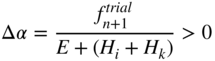
Using the preceding equation and the third and fifth equations in Equation 25, the incremental variable Δα > 0 can be determined from the fifth equation of Equation 25 as follows:

In this equation, ![]() , which can be evaluated based on the information known from the previous step. The preceding equation then yields
, which can be evaluated based on the information known from the previous step. The preceding equation then yields
Using Equations 29 and 31, all the unknowns in Equation 25, σn+1, ![]() , αn+1, and qn+1, can be determined. That is, the use of the return mapping algorithm in this simple case allows determining all the unknowns in a closed form.
, αn+1, and qn+1, can be determined. That is, the use of the return mapping algorithm in this simple case allows determining all the unknowns in a closed form.
For von Mises plasticity, the yield surface is circular, and as a result, the normal to the yield surface is radial. In this special case, the general return mapping algorithm reduces to the popular radial return mapping algorithm.
8.4 GENERALIZATION OF THE PLASTICITY THEORY: SMALL STRAINS
The one-dimensional plasticity theory presented in the preceding sections can be generalized and used in the three-dimensional analysis (Simo and Hughes, 1998). To this end, the same notation previously used will be used in this section, except bold letters are used to denote vectors, matrices, and tensors that replace the scalar variables used in the one-dimensional theory. Because in this section, the additive decomposition of the strain rate is used, strains are assumed small and there is no distinction made between different stress measures. For this reason, Cauchy stress tensor is used in this section with the Green–Lagrange strain tensor. Furthermore, the objectivity requirement is not an issue in the small-strain formulation. The formulation presented in this section can be used with hypoelastic material models and does not require that the stress–strain relationships are obtained from a potential function as in the case of hyperelastic material models.
The stress–strain relationship can be written as
In this equation, E is the fourth-order tensor of elastic coefficients, σ is the second-order stress tensor, ϵ is the second-order total strain tensor, ϵe is the second-order tensor of elastic strains, and ϵp is the second-order tensor of plastic strains. The elastic domain is defined by
where q is the vector of the internal variables that depend on the plastic strains and a set of hardening parameters α. These internal variables account in this case for both the kinematic and isotropic hardening. The general nonassociative model flow rule and hardening law are defined as

where g and h are prescribed second-order tensor functions of σ and q, and γ is the consistency parameter.
Based on the analysis used in the case of the one-dimensional model, the Kuhn–Tucker loading and unloading complementarity condition for the more general three-dimensional case can be written as
The consistency condition is
This consistency condition, ![]() , can be used to determine the consistency parameter. This condition defines γ, as shown in the following example, as
, can be used to determine the consistency parameter. This condition defines γ, as shown in the following example, as

In this equation, fσ and fq are second-order tensors that result from the differentiation of the yield function ![]() with respect to σ and q, respectively. It is assumed that the denominator in the preceding equation is always greater than zero, an assumption that always holds for associative plasticity.
with respect to σ and q, respectively. It is assumed that the denominator in the preceding equation is always greater than zero, an assumption that always holds for associative plasticity.
Because of the assumption of small deformation, the stress rate can be written as
Substituting Equation 37 into this equation, one obtains
where Eep is the tensor of tangent elastoplastic moduli given by

Note the incremental nature of the plasticity formulation because of the rate form of Equation 39. Note also that in the general case of nonassociative plasticity, the tangent elastoplastic moduli tensor is not necessarily symmetric. In the actual implementation, if there is no need to evaluate the tensor of Equation 40, one can simply determine the stress rate by substituting the scalar γ of Equation 37 into Equation 38. In this case, the use of the tensor multiplication given in Equation 40 can be avoided.
Associative Plasticity
In the special case of associative plasticity, one has the following assumptions:

where in this equation Dp is the matrix of generalized plastic moduli. The preceding equation implies that g = ∂f/∂σ and the plastic flow is in the direction of the normal to the yield surface. Using the assumptions of associative plasticity, it can be shown that the denominator in the right-hand side of Equation 37 that also appears in Equation 40 is greater than zero, as previously mentioned. It is also clear from Equation 40 that in the case of associative plasticity, the tangent elastoplastic moduli tensor is symmetric.
Numerical Solution of the Plasticity Equations
In the remainder of this section, the procedure used to solve the nonassociative plasticity equations presented in this section is described. The numerical procedure for integrating the plasticity equations is called the constitutive integration algorithm or the stress update algorithm. A class of solution algorithms that are widely used in the solution of the plasticity equations is the return mapping algorithms that are discussed in this section. It is, however, important to point out that in the case of the large-deformation plasticity formulations discussed in later sections of this chapter, the objectivity requirements need to be satisfied by the rate constitutive equations.
For nonassociative plasticity, the equations for small-strain elastoplasticity can be summarized as follows:

Assume that at time tn, σn, ϵn, ![]() , and qn are known, where subscript n refers to the time-step. The goal is to use the preceding equations to determine the states of stresses and strains at time tn+1 that satisfy the loading and unloading conditions. From the solution of the dynamic equations, ϵn+1 and Δϵ = ϵn+1 − ϵn are known.
, and qn are known, where subscript n refers to the time-step. The goal is to use the preceding equations to determine the states of stresses and strains at time tn+1 that satisfy the loading and unloading conditions. From the solution of the dynamic equations, ϵn+1 and Δϵ = ϵn+1 − ϵn are known.
Explicit Solution
Let the plasticity parameter γ = ![]() , with Δα = γΔt. It was shown previously that the use of the consistency condition leads to (Equation 37)
, with Δα = γΔt. It was shown previously that the use of the consistency condition leads to (Equation 37)

One may consider, as it was the case in some of the early work on computational plasticity, to use this value of the plasticity parameter to update the plastic strains, internal variables, and stresses using a simple explicit one-step Euler method as follows:

There is no guarantee, however, that this explicit updating scheme, sometimes referred to as tangent modulus update scheme, will satisfy the yield condition. Therefore, the use of the explicit scheme as defined by Equation 44 is not recommended. Instead, one can use the implicit method described in the following paragraph to obtain a more accurate solution.
Implicit Solution
Using an implicit integration method, the first four equations in Equation 42 can be converted to a set of nonlinear algebraic equations. These algebraic equations, in principle, can be solved iteratively using a Newton–Raphson algorithm, as in the one-dimensional case, to determine σ, ϵp, q, and γ. Nonetheless, one can try to take advantage of the structure of the plasticity equations in order to develop an effective and more efficient algorithm for the three-dimensional plasticity problems. In order to ensure that the yield condition is satisfied, the return mapping algorithms are used. In the return mapping algorithms, as in the case of the one-dimensional model, an initial elastic predictor step that may give a solution away from the yield surface is first used. A plastic corrector step is then used to bring the solution to the updated yield surface. In the return mapping algorithms, as previously mentioned, a simple numerical integration method such as the trapezoidal rule, Runge–Kutta method, or the midpoint method is first used to transform the plasticity differential equations into a set of nonlinear algebraic equations that can be solved using a Newton–Raphson algorithm to determine the stresses, strains, and internal variables at time tn+1. For example, if the fully implicit backward Euler method is used as the numerical integrator, the equations are written in terms of variables defined at the end of the time-step. This leads to

where again γ Δt = Δα. One may choose to work directly with these four sets of equations, or eliminate some unknowns before starting the numerical procedure. For example, the plastic strains can be eliminated by using the constitutive equations. In this case, one can write the plastic strain tensor ![]() in terms of the stress tensor σn+1 as
in terms of the stress tensor σn+1 as
This equation can be used to eliminate ![]() from Equation 45 and obtain the following reduced system of nonlinear algebraic equations
from Equation 45 and obtain the following reduced system of nonlinear algebraic equations

where Ei is the fourth-order tensor used to write the strain components in terms of the stress components (inverse relationship). This system of nonlinear algebraic equations can be solved using the iterative Newton–Raphson method in order to determine σn+1, qn+1, and Δα. This requires constructing and iteratively solving the following system:

In this equation, ![]() is used to denote Newton differences. Note that the increment of the plastic strains can be written as
is used to denote Newton differences. Note that the increment of the plastic strains can be written as
which upon substituting into the stress equation yields

The trial stress of the elastic predictor step is defined as
which upon substituting into Equation 50, one obtains
In this equation
is the plastic corrector that brings the trial stress to the yield surface along a direction specified by the plastic flow direction. During the elastic predictor step, the plastic strains and the internal variables remain fixed, whereas during the plastic corrector step, the total strain is fixed (Belytschko et al., 2000). It follows from the preceding equation that
In the solution procedure described in this section, the total strain is assumed to be fixed while the plasticity equations are solved for stresses, plastic strains, internal hardening variables, and consistency parameter. Consequently, the values of the elastic strains will depend on the values of the plastic strains obtained using the plasticity equations. The elastic strains can be determined using the strain additive decomposition as ϵe = ϵ − ϵp. In the large deformation theory, this additive decomposition is not used. Before introducing the large deformation theory, a J2 flow theory based on the small-strain assumptions is first discussed.
8.5 J2 FLOW THEORY WITH ISOTROPIC/KINEMATIC HARDENING
A special case of the small-strain three-dimensional formulation presented in the preceding sections is the J2 flow theory. This theory that is based on the von Mises yield surface is useful, particularly in the plasticity analysis of metals. The main assumption used in this theory is that the plastic flow is not affected by the hydrostatic pressure as was experimentally demonstrated (Bridgman, 1949). Using this assumption, the yield condition and the plastic flow are formulated in terms of the deviatoric stresses. The yield function in this case becomes a function of only the second invariant of the deviatoric stresses J2.
In the J2 flow theory with isotropic and kinematic hardening, the set of internal variables ![]() is introduced (Simo and Hughes, 1998). Here, α is the equivalent plastic strain that defines the isotropic hardening of the von Mises yield surface and
is introduced (Simo and Hughes, 1998). Here, α is the equivalent plastic strain that defines the isotropic hardening of the von Mises yield surface and ![]() defines the kinematic hardening variables in the stress deviator space in the case of the von Mises yield surface. Let
defines the kinematic hardening variables in the stress deviator space in the case of the von Mises yield surface. Let
In this equation, S is the stress deviator. Note that the trace of the tensor ![]() is assumed to be equal to zero. The resulting J2 plasticity model is governed by the following equations (Zienkiewicz and Taylor, 2000):
is assumed to be equal to zero. The resulting J2 plasticity model is governed by the following equations (Zienkiewicz and Taylor, 2000):

where ![]() . In this equation, γ is the consistency parameter; the functions Hi(α) and Hk(α) are, respectively, the isotropic and kinematic hardening moduli; and
. In this equation, γ is the consistency parameter; the functions Hi(α) and Hk(α) are, respectively, the isotropic and kinematic hardening moduli; and ![]() is the plastic strain tensor deviator. The yield function defined by the first equation in Equation 56 is called the Huber–von Mises yield function. In many applications, particularly in the case of metals, the isotropic hardening modulus Hi(α) is assumed to be the linear function of α. In this special case, Hi(α) can be written as
is the plastic strain tensor deviator. The yield function defined by the first equation in Equation 56 is called the Huber–von Mises yield function. In many applications, particularly in the case of metals, the isotropic hardening modulus Hi(α) is assumed to be the linear function of α. In this special case, Hi(α) can be written as ![]() , where σy is the yield stress and
, where σy is the yield stress and ![]() , is a constant. On the other hand, if the kinematic hardening modulus Hk(α) is assumed to be constant, one has the Prager–Ziegler rule. The reader may also notice the similarity between the third equation in Equations 56 and 7 in the simple case of the one-dimensional theory. The factor
, is a constant. On the other hand, if the kinematic hardening modulus Hk(α) is assumed to be constant, one has the Prager–Ziegler rule. The reader may also notice the similarity between the third equation in Equations 56 and 7 in the simple case of the one-dimensional theory. The factor ![]() is introduced in Equation 56 in order to match the behavior of the metals in the case of uniaxial testing (Zienkiewicz and Taylor, 2000).
is introduced in Equation 56 in order to match the behavior of the metals in the case of uniaxial testing (Zienkiewicz and Taylor, 2000).
It is clear from the second equation in Equation 56 that ![]() . Using this fact, the last equation in Equation 56 yields
. Using this fact, the last equation in Equation 56 yields

This equation defines the relationship between α and the norm of the plastic-strain-rate deviator (Simo and Hughes, 1998).
As discussed in the general small deformation plasticity theory, the differential equations associated with ![]() ,
, ![]() , and
, and ![]() can be augmented with a constitutive equation in a rate form. In the case of the J2 plasticity, the constitutive equations for the stress deviator are used. The elastic deviatoric stress–strain relation can be written as
can be augmented with a constitutive equation in a rate form. In the case of the J2 plasticity, the constitutive equations for the stress deviator are used. The elastic deviatoric stress–strain relation can be written as
where μ is the shear modulus (Lame's constant), ϵd is the strain deviator, ![]() is the elastic strain deviator, and
is the elastic strain deviator, and ![]() is the plastic strain deviator. Note that the strain additive decomposition is used in the preceding equation, and consequently, the development presented in this section can be used for small-strain problems only. Differentiating the preceding equation, and using Equation 56, one obtains
is the plastic strain deviator. Note that the strain additive decomposition is used in the preceding equation, and consequently, the development presented in this section can be used for small-strain problems only. Differentiating the preceding equation, and using Equation 56, one obtains
and
Because the tr(n) = 0, one has ![]() . In Equation 59,
. In Equation 59, ![]() is assumed to be known because the strain and strain rate are assumed to be known. On the other hand, the stress and plastic strain deviators are unknowns, and they are to be determined by solving the plasticity equations.
is assumed to be known because the strain and strain rate are assumed to be known. On the other hand, the stress and plastic strain deviators are unknowns, and they are to be determined by solving the plasticity equations.
Equation 59 with the last three equations of Equation 56 defines four sets of first-order differential equations that can be, in principle, solved for the unknowns S, ![]() ,
, ![]() , and α. In the most general J2 plasticity formulations, an integration method can be used to transform these differential equations into a set of nonlinear algebraic equations, which can be solved simultaneously for the unknowns as previously discussed in this chapter. The first equation in Equation 56 can be used to determine the consistency parameter γ, as will be discussed later in this section.
, and α. In the most general J2 plasticity formulations, an integration method can be used to transform these differential equations into a set of nonlinear algebraic equations, which can be solved simultaneously for the unknowns as previously discussed in this chapter. The first equation in Equation 56 can be used to determine the consistency parameter γ, as will be discussed later in this section.
It is important, however, before presenting the form of the consistency parameter to realize that the J2 plasticity theory can be formulated also in terms of the stress tensor instead of the deviatoric stress tensor. Recall that σ = S + pI, where p is the hydrostatic pressure. Therefore, if the deviatoric stress S and the hydrostatic pressure p are known, the stress tensor σ can be determined. The hydrostatic pressure can be obtained using an elastic relationship between the volumetric strain, which is assumed to be known, and bulk modulus. Furthermore, if the rate of the stress deviator is known, one can obtain the rate of the stress tensor using the following equation:
The general form of the consistency parameter given by Equation 37 reduces the case of J2 plasticity, as demonstrated in the following example, to

Finally, for γ ≥ 0, one can show that the elastoplastic tangent moduli in the case of plastic loading can be obtained from the use of the preceding equation or alternatively by using Equation 40 as

In this equation, K is bulk modulus, and Ik is the kth-order identity tensor. Equation 63 is obtained assuming that the hydrostatic pressure p is related to the volumetric strain ϵt using the linear elastic relation p = Kϵt.
Nonlinear Isotropic/Kinematic Hardening
The procedure used to solve the J2 plasticity equations in the general case of isotropic and kinematic hardening is first outlined. The special case of linear isotropic and kinematic hardening is also discussed before concluding this section.
Using the J2 flow theory presented in this section, one can use the implicit backward Euler method to transform the first-order differential equations to a set of algebraic equations that are similar to Equations 47 and 48. It can be, however, shown that one only needs to solve one scalar nonlinear equation in order to determine the state of stress and strains at time tn+1. To this end, the implicit backward Euler method can be used with Equations 55 and 56 to obtain

where ![]() . In Equation 64, Δϵd = (ϵd)n+1 − (ϵd)n is assumed to be known because the total strain at time tn+1 is assumed to be known. Note also that the unknowns on the left-hand side of Equation 64 can be determined if nn+1 and Δy are determined. To this end, the trial stress state can be defined by the following equations:
. In Equation 64, Δϵd = (ϵd)n+1 − (ϵd)n is assumed to be known because the total strain at time tn+1 is assumed to be known. Note also that the unknowns on the left-hand side of Equation 64 can be determined if nn+1 and Δy are determined. To this end, the trial stress state can be defined by the following equations:

These trial solutions are function of known variables defined at time tn.
In the following, it is shown that, if nn+1 can be determined, the solution of Equation 64 reduces to the solution of a nonlinear scalar equation for the consistency parameter Δγ. Because ![]() , where 2 μ(Δγ nn+1) is the plastic corrector,
, where 2 μ(Δγ nn+1) is the plastic corrector, ![]() can be expressed in terms of
can be expressed in terms of ![]() using the following equation:
using the following equation:

Substituting ηn+1 = ||ηn+1|| ηn+1 in the preceding equation shows that ![]() and nn+1 are in the same direction and, therefore, nn+1 can be written in terms of the trial elastic stress
and nn+1 are in the same direction and, therefore, nn+1 can be written in terms of the trial elastic stress ![]() as
as

This equation shows that nn+1 can be evaluated using information available at time tn. Therefore, the only remaining unknown on the left-hand side of Equation 64 is Δγ. If Δγ is determined, the state of stresses and strains at time tn+1 can be determined using Equation 64. To this end, one can take the double contraction of Equation 66 with nn+1 and recall in the plastic state that ![]() , which is the result of the yield condition (see the first equation in Equation 56). One can then obtain the following scalar equation in Δγ:
, which is the result of the yield condition (see the first equation in Equation 56). One can then obtain the following scalar equation in Δγ:

The first term on the right-hand side of this equation is the result of the fact that nn+1 and ηn+1 are in the same direction and the following identity: ![]() . The nonlinear equation of Equation 68 can be solved using a local Newton–Raphson iterative procedure. The convergence is guaranteed because the function is convex as the result of using the associative plasticity model (Simo and Hughes, 1998). Knowing Δγ and using Equation 67, all the unknowns in Equation 64 as well as the stress at time tn+1 can be determined.
. The nonlinear equation of Equation 68 can be solved using a local Newton–Raphson iterative procedure. The convergence is guaranteed because the function is convex as the result of using the associative plasticity model (Simo and Hughes, 1998). Knowing Δγ and using Equation 67, all the unknowns in Equation 64 as well as the stress at time tn+1 can be determined.
The relationship between the stresses and strains in the plasticity formulation discussed in this section can be written as follows:
The incremental form of this equation can be written as

where ![]() is the elasticity tensor. Note that
is the elasticity tensor. Note that
In the general case, the term ∂(Δγ)/∂ϵn+1 in Equation 70 can be obtained from the differentiation of Equation 68. The incremental form of Equation 70 can be used to determine the consistent tangent moduli that define the relationship between the stresses and the total strains.
Return Mapping Algorithm for Nonlinear Isotropic/Kinematic Hardening
Based on the discussion presented in this section, the following algorithm can be summarized in the case of the J2 plasticity theory that accounts for nonlinear isotropic and kinematic hardening (Simo and Hughes, 1998):
- 1. Using the fact that the strain is known at time tn+1 and using the information at time tn compute the deviatoric strain tensor and the trial elastic stresses using the following equations:
8.72

- 2.
Check the yield condition by evaluating the following Huber–von Mises function:
8.73
If
 , an elastic state is assumed. In this case, set the plasticity variables at tn+1 equal to the plasticity variables at tn, determine the stresses using the elastic relationships, and exit.
 - 3. If
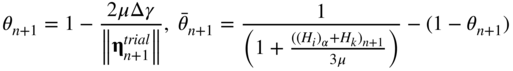
 , solve the plasticity equations. Compute nn+1 and find Δγ from the solution of Equation 68. In this case, one has
8.74
, solve the plasticity equations. Compute nn+1 and find Δγ from the solution of Equation 68. In this case, one has
8.74
- and
8.75

- 4. Update the back stress, plastic strain, and stress tensors using the following equations:
8.76

- 5. The consistent elastoplastic tangent moduli can be computed using the formula (Simo and Hughes, 1998)
8.77

- where
8.78
This algorithm requires the solution of one nonlinear algebraic equation (Equation 68). In the finite element implementation, this equation needs to be solved at the integration points.
There are important considerations that must be taken into account when implementing the algorithm presented in this section. The following important remarks can be made regarding the proposed algorithm (Simo and Hughes, 1998):
- 1. In the analysis presented in this section, the backward Euler method was used as an example to obtain the nonlinear plasticity algebraic equations. Nonetheless, other implicit integration methods can be used to transform the first-order differential equations into a set of nonlinear algebraic equations. In particular, the backward Euler method can be replaced by the generalized midpoint rule in the derivation of the discrete equations as proposed by Ortiz and Popov (1985) or Simo and Taylor (1986). For the J2 flow theory, this results in the return map proposed by Rice and Tracey (1973).
- 2. Note that the values of the variables at step n + 1 are calculated based solely on the converged values at step n. Use of an iterative scheme based on intermediate nonconverged values is questionable for a problem that is physically path dependent.
- 3. In the computer implementation, the expression for the consistent tangent moduli should be compared with the “continuum” elastoplastic tangent moduli in order to estimate the errors. For large time-steps, the consistent tangent moduli may differ significantly from the “continuum” elastoplastic tangent moduli.
Linear Kinematic/Isotropic Hardening
In metal plasticity applications, it is often assumed that the isotropic hardening is linear of the form ![]() where
where ![]() , is a constant. Alternatively, one can use the following form of combined kinematic/isotropic hardening laws (Hughes, 1984):
, is a constant. Alternatively, one can use the following form of combined kinematic/isotropic hardening laws (Hughes, 1984):
where ![]() is a constant. As previously mentioned, the assumption of a constant kinematic hardening modulus is known as Prager–Ziegler rule. More general isotropic hardening models can also be used (Hughes, 1984).
is a constant. As previously mentioned, the assumption of a constant kinematic hardening modulus is known as Prager–Ziegler rule. More general isotropic hardening models can also be used (Hughes, 1984).
In the special case of linear kinematic/isotropic hardening, one has

where β ∈ [0, 1] and ![]() is a given material hardening parameter. In this special case, a closed-form solution for Δγ can be obtained by substituting the preceding equation into Equation 68 and assuming that
is a given material hardening parameter. In this special case, a closed-form solution for Δγ can be obtained by substituting the preceding equation into Equation 68 and assuming that ![]() . This leads to
. This leads to

Using this result, the update procedure is completed by substituting Equation 81 into Equation 64.
8.6 NONLINEAR FORMULATION FOR HYPERELASTIC–PLASTIC MATERIALS
The elastic response of hyperelastic materials is derived from a potential function and, therefore, the work done in a deformation process is path independent. This is not the case when hypoelastic models are used. For hypoelastic materials, the elastic response is not derived from a potential function and the work done in a deformation process is path dependent. For all inelastic materials, the constitutive equations depend on the path followed in a deformation process. It is, therefore, important to follow this path in order to be able to accurately determine the current state of stresses. This is also clear from the mathematical fact that the solution of algebraic equations does not require knowledge of the history, whereas the solution of differential equations requires knowledge of variable history. Similarly, the evaluation of an integral requires one to define the limits of integration. The numerical evaluation of an integral, for example, requires information at several past points, and not only information at the current point.
When hypoelastic–plastic models are used, the yield function is required to be an isotropic function of the stress, and the objectivity requirements restrict the elastic moduli to be isotropic if these moduli are assumed to be constant (Belytschko et al., 2000). Furthermore, the numerical solution of the plasticity equations based on the hypoelastic–plastic formulations requires the use of incrementally objective integration schemes. There are in the literature formulations of hypoelastic materials for large strains based on the additive decomposition of the rate of deformation tensor (Belytschko et al., 2000). It is assumed in these formulations, however, that the elastic strains are small compared to the plastic strains. Furthermore, energy is not conserved in a closed deformation cycle. Such an energy violation, however, can be insignificant if the assumption of small elastic strains is observed. The use of a hyperelastic–plastic formulation, on the other hand, relaxes these requirements. In this section, the formulation of the constitutive equations for hyperelastic–plastic materials in the case of large strains is presented.
Multiplicative Decomposition
The multiplicative decomposition of the matrix of the position vector gradients, instead of the additive form assumed for small strains, is the basis for the theory developed in this section for hyperelastic–plastic materials (Bonet and Wood, 1997). Recall that a line element dx in the reference configuration corresponds to a line element dr in the current configuration. If the material is elastic and the load is removed, dx and dr differ only by a rigid-body rotation. If the material, on the other hand, experiences a plastic deformation, a certain amount of permanent deformation remains upon the removal of the load, and dr will correspond to the vector drp' in a stress-free intermediate configuration called in this book the intermediate plastic configuration as shown in Figure 1. The relationship between dx and dr is given by the matrix of the position vector gradients J, whereas the relationship between dx and drp is given by the matrix of the position vector gradients Jp. The relationship between drp and dr is given by the matrix of the position vector gradients Je. These kinematic relationships are defined for an arbitrary element dx as

Figure 8.1 Intermediate plastic configuration
From these equations, it is clear that
This equation is the multiplicative decomposition of the matrix of position vector gradients into an elastic part Je and a plastic part Jp.
Using the multiplicative decomposition, strain measures that are independent of the rigid-body displacements can be defined. For example, the following right Cauchy–Green strain tensors for the total, elastic, and plastic deformations can be defined as
These tensors are often used in the formulation of the constitutive equations of plastic materials. Because Cr measures the total strains and ![]() measures the plastic strains, both tensors are required in order to completely describe the current state of the material. Using the preceding equation, an elastic Green–Lagrange strain tensor that measures the elastic deformation from the stress-free intermediate plastic configuration to the current configuration can be defined as
measures the plastic strains, both tensors are required in order to completely describe the current state of the material. Using the preceding equation, an elastic Green–Lagrange strain tensor that measures the elastic deformation from the stress-free intermediate plastic configuration to the current configuration can be defined as
Under a superimposed rigid-body rotation from the current configuration, the final matrix of the position vector gradients from the stress-free intermediate plastic configuration is ![]() , where A is the rotation matrix. It follows that ϵe is invariant under and is not affected by the rigid-body rotation, a property similar to that of the second Piola–Kirchhoff stress tensor as discussed in Chapter 3.
, where A is the rotation matrix. It follows that ϵe is invariant under and is not affected by the rigid-body rotation, a property similar to that of the second Piola–Kirchhoff stress tensor as discussed in Chapter 3.
For isotropic materials, it is sometimes simpler to develop the constitutive equations in the current configuration using the elastic left Cauchy–Green tensor given as
It can be shown that the potential function used in a hyperelastic model can be written in terms of the invariants of ![]() .
.
Hyperelastic Potential
In the case of large deformations, it is important to distinguish between different stress and strain measures. Associated with the elastic strain tensor ϵe, one can define the second Piola–Kirchhoff stress tensor ![]() as the pullback of the Kirchhoff stress tensor σK as
as the pullback of the Kirchhoff stress tensor σK as
Kirchhoff stress is used here instead of Cauchy stress because Truesdell rate of Kirchhoff stress is the push-forward of the rate of the second Piola − Kirchhoff stress as demonstrated in Chapter 3. Recall that Kirchhoff stress tensor differs from Cauchy stress tensor by a scalar multiplier, which is the determinant of the matrix of the position vector gradients.
For the hyperelastic material plasticity model discussed in this section, it is assumed that the stress–strain relationships can be obtained from a strain-energy function formulated relative to the intermediate plastic configuration. Using this assumption, the second Piola − Kirchhoff stress tensor can be derived from an energy potential function Ue as

Taking the derivatives of this equation with respect to time, one obtains

where Ee is the matrix of elastic coefficients that relates the rate of the second Piola − Kirchhoff stress tensor ![]() to the rate of the elastic Green–Lagrange strain tensor ϵe. Note that both
to the rate of the elastic Green–Lagrange strain tensor ϵe. Note that both ![]() and ϵe are invariant under a superimposed rigid-body motion. Therefore, using these two tensors ensures that the elastic response is objective. The preceding equation also shows that Ee does not change under a rigid-body rotation and, therefore, the elastic moduli can be anisotropic, unlike the case of hypoelastic models.
and ϵe are invariant under a superimposed rigid-body motion. Therefore, using these two tensors ensures that the elastic response is objective. The preceding equation also shows that Ee does not change under a rigid-body rotation and, therefore, the elastic moduli can be anisotropic, unlike the case of hypoelastic models.
Rate of Deformation Tensors
In the hyperelastic − plastic formulation discussed in this section, the plasticity equations are expressed in terms of the rate of deformation tensors defined in the intermediate plastic configuration (Simo and Hughes, 1998; Belytschko et al., 2000). In order to determine expressions for these tensors, the matrix of velocity gradients is written as
This equation can be written as the sum of elastic and plastic parts as
where
This equation shows that the elastic part Le has the usual form of the matrix of the velocity gradients expressed in terms of Je instead of J, whereas the plastic part Lp is pushed forward by Je. One can define the symmetric and the skew-symmetric parts of Le and 1 Lp as follows:

The velocity gradient L can be pulled back by Je to the intermediate plastic configuration defining the velocity gradient ![]() as follows:
as follows:
In this equation,
are the elastic and plastic parts of ![]() . One can also obtain
. One can also obtain ![]() using the elementary definition of Equation 82 as
using the elementary definition of Equation 82 as ![]() , where vp = drp/dt.
, where vp = drp/dt.
Similarly, the following symmetric rate of deformation tensors can be defined as the pullback of D, De, and Dp by Je to the intermediate plastic configuration (Belytschko et al., 2000):

Note that by using these definitions, one has ![]() . Because
. Because ![]() , one has
, one has
This equation, upon using the previously given definitions of ![]() (Equation 96),
(Equation 96), ![]() (Equation 84), and
(Equation 84), and ![]() (Equation 95), leads to
(Equation 95), leads to
Therefore, the stress rate ![]() can be written using the relationship
can be written using the relationship ![]() presented previously in this section for hyperelastic materials (Equation 89) as
presented previously in this section for hyperelastic materials (Equation 89) as
This equation, which takes a simple form as the result of using the definitions of Equation 96, will be used to define the elastic–plastic tangent moduli. It is important, however, to point out that the use of the additive decomposition of rates of deformation measures does not impose a restriction on the applicability of the formulation presented in this section to large deformation problems. This argument is similar to the one used when dealing with rotations. Although finite rotations cannot be added, the angular velocities can be added. Recall that the angular velocities are not in general the time derivatives of orientation parameters. Similarly, some of the rates of the deformation measures are also not in general exact differentials.
Flow Rule and Hardening Law
In the case of the large deformations, the elastic domain can be defined in terms of the stresses and the internal plasticity variables as
In this equation, q is a set of internal variables. Because ![]() is invariant under a superimposed rigid-body rotation, objectivity imposes no restrictions on the yield function allowing for the use of anisotropic plastic model.
is invariant under a superimposed rigid-body rotation, objectivity imposes no restrictions on the yield function allowing for the use of anisotropic plastic model.
The general nonassociative model flow rule and hardening law are defined as

where g and h are prescribed functions. Note that, because of the definition of ![]() , g is a tensor defined in the intermediate plastic configuration. In the flow rule,
, g is a tensor defined in the intermediate plastic configuration. In the flow rule, ![]() is used instead of the plastic part of the rate of deformation tensor Dp as it is the case in some hypoelastic–plastic models.
is used instead of the plastic part of the rate of deformation tensor Dp as it is the case in some hypoelastic–plastic models.
The Kuhn–Tucker loading and unloading complementarity condition can be written as
The consistency condition is
The consistency condition ![]() can be used to determine the consistency parameter as follows:
can be used to determine the consistency parameter as follows:

In this equation,
is obtained from the definition of ![]() in the flow rule. Note also that
in the flow rule. Note also that
Substituting these results into the constitutive equations (Equation 99), one obtains
This equation can be written as
where Eep is the tensor of tangent elastoplastic moduli given by

In the general case of nonassociative plasticity, the tangent elastic–plastic moduli tensor is not necessarily symmetric. It is symmetric in the case of associative plasticity. It is important to reiterate that the objectivity requirements are automatically satisfied for hyperelastic–plastic formulations because the elastic strains and stresses used in this formulation are invariant under a superimposed rigid-body motion. In order to demonstrate this fact, one follows a procedure similar to the procedure used in the preceding chapter by assuming A to be a time-dependent rigid-body rotation from the current configuration. Note that the reference and intermediate plastic configurations are not affected by this rotation. It follows that the new matrix of position vector gradients is given by AJ, whereas the elastic part will be AJe and the plastic part will remain Jp. Consequently, the elastic Lagrangian strain ϵe will remain the same. Consequently, the stresses are not affected by the rotation because they can be directly evaluated using Equation 88 and no integration of stress rate is required.
Numerical Solution
It is assumed that the matrix of position vector gradients J and the Green–Lagrange strain tensor ϵ are known. It follows then that the matrix Je can be expressed in terms of the matrix Jp as ![]() . Therefore, it can be shown that
. Therefore, it can be shown that ![]() ,
, ![]() , and
, and ![]() in Equations 99 and 101 can be expressed in terms of Jp. As a result, Equations 99–101 represent a set of four systems of equations that can be solved for the unknowns
in Equations 99 and 101 can be expressed in terms of Jp. As a result, Equations 99–101 represent a set of four systems of equations that can be solved for the unknowns ![]() , Jp, q, and γ. To this end, the implicit backward Euler method can be used to convert the system of differential equations to a set of nonlinear algebraic equations that can be solved using the iterative Newton–Raphson method as described previously in this chapter. It is important to point out, however, that Jp is not necessarily symmetric, and
, Jp, q, and γ. To this end, the implicit backward Euler method can be used to convert the system of differential equations to a set of nonlinear algebraic equations that can be solved using the iterative Newton–Raphson method as described previously in this chapter. It is important to point out, however, that Jp is not necessarily symmetric, and ![]() ,
, ![]() , and
, and ![]() in the general theory presented in this section are not simple functions of Jp. For this reason, the numerical solution of the general equations of the hyperelastic–plastic model can be less efficient compared with cases in which a closed-form solution can be obtained.
in the general theory presented in this section are not simple functions of Jp. For this reason, the numerical solution of the general equations of the hyperelastic–plastic model can be less efficient compared with cases in which a closed-form solution can be obtained.
Rate-Dependent Plasticity
In the case of rate-dependent plasticity, γ is defined as

In this equation, η is the viscosity and φ is an overstress function. The relationship between the stress and rate of deformation tensor can be written as

More discussion on the rate-dependent plasticity formulations can be found in the reference by Simo and Hughes (1998).
8.7 HYPERELASTIC–PLASTIC J2 FLOW THEORY
In this section, the hyperelastic–plastic formulation based on the J2 flow theory is discussed. The use of this theory leads to a simple integration algorithm, which can be considered as an extension of the radial return mapping algorithm used for the infinitesimal J2 flow theory. The development of the formulation is illustrated using a model based on the Neo-Hookean material that is suited for the analysis of large deformation. The main assumptions used in the J2 flow theory as compared to the general theory presented in the preceding section are that plastic spin is zero and the yield condition is a function of the deviatoric part of the stress only and does not depend on the hydrostatic pressure. Using these two assumptions, the formulation presented in the preceding section can be systematically specialized to the case of the J2 flow theory.
For the Neo-Hookean material, the energy potential function can be written in the intermediate plastic configuration as
where ![]() is the first principal invariant of the tensor
is the first principal invariant of the tensor ![]() , Je = |Je| = det(Je), and λe and μ are Lame's constants. The second Piola–Kirchhoff stress tensor is obtained as described in Chapter 4 as
, Je = |Je| = det(Je), and λe and μ are Lame's constants. The second Piola–Kirchhoff stress tensor is obtained as described in Chapter 4 as
This equation can be used to obtain the following rate form of hyperelasticity:
The deviatoric stress tensor associated with the intermediate plastic configuration can also be defined as described in Chapter 4 as
The elastic domain is defined by the von Mises yield surface
In the J2 flow theory presented in this section, it is assumed that the plastic spin ![]() is identically equal to zero. Therefore, the flow rule can be written in terms of the symmetric part
is identically equal to zero. Therefore, the flow rule can be written in terms of the symmetric part ![]() , instead of
, instead of ![]() , using the assumptions of associative plasticity as (Belytschko et al., 2000)
, using the assumptions of associative plasticity as (Belytschko et al., 2000)

In this equation, gs is obtained using Equation 105 where g is defined in the intermediate plastic configuration, and σe is the von Mises effective stress defined as

Using the equations presented in this section, the elastoplastic tangent moduli can be obtained by substituting in the form presented in the preceding section.
PROBLEMS
-
1 Explain the Bauschinger Phenomenon.
-
2 Define the basic hypotheses on which the theory of plasticity is based.
-
3 Define the isotropic and kinematic hardening.
-
4 What is the difference between associative and nonassociative plasticity?
-
5 What is the difference between the return mapping algorithm and the radial return mapping algorithm?
-
6 What are the drawbacks of using explicit integration instead of implicit integration to solve the plasticity equations?
-
7 Outline in detail the steps of a numerical solution of the plasticity equations of the hyperelastic material model discussed in Section 6.
-
8 Discuss the main assumptions used in the J2 flow theory for the hyperelastic model presented in Section 7 as compared to the more general model presented in Section 6.
-
9 Outline in detail the steps of a numerical solution that can be used for the J2 flow theory for the hyperelastic model presented in Section 7.