CHAPTER 10
Natural Resources and Ecosystem Services
10.0 Introduction
You may be reading this book from the comfort of your apartment, or perhaps in a coffee shop, library, or office. Wherever you are, surrounded by human-made things, it is easy to think that we are not dependent on natural capital. But think more deeply. Your chair is made of wood or metal and covered with cloth or leather. Your building is heated or air-conditioned by the combustion of fossil fuels; or nuclear power, which uses uranium as a fuel source; or renewable energy such as wind or solar power. You likely drove to your current location in a gasoline-powered car or bus, assembled from various metals, rubber, and plastic made from oil or other hydrocarbons. The cell phone that you carry around contains small amounts of beryllium, cadmium, cobalt, copper, lead, mercury, nickel, palladium, silver, and zinc. Although many economics textbooks depict production as being dependent on capital, by which it is usually meant manufactured capital (industrial plant and equipment), and labor, we are, in fact, utterly and totally dependent on natural resources.
The previous two chapters have focused on sustainability as the goal of our economy. As we have seen, an important determinant of whether society is achieving sustainability is whether we are leaving the next generation with suitable capital stocks, including stocks of natural resources. (Note: by stocks, in this chapter, we mean physical stocks of resources—trees, minerals in the ground, and fish in the ocean—not stocks as pieces of paper representing ownership in a company.) Here, we dive deeper into the economic issues surrounding our use of natural resources.
“Natural Resources” comprise a huge category, including all of the raw materials that sustain human well-being that are not directly made by humans. All manufactured capital and all final goods and services, ultimately depend on some sort of natural resource, which is one form of “natural capital.” Natural capital also includes ecological processes that underlie the provision of ecosystem services. In this chapter, we explore the economics of three broad classes of natural capital: nonrenewable resources, renewable resources, and ecological processes undergirding ecosystem services.
Nonrenewable resources are resources in fixed supply such as oil, coal, or minerals. Over the long arc of geologic time, millions of years, more oil or coal will be produced, so in a sense these resources are really very slowly renewing resources. But for practical purposes, at least in thinking about things over the next 1,000 years, we have the oil and coal supply that we have, and nature will produce no more. Renewable resources, by contrast, are biological resources for which there is a natural growth function. Fish, game species, trees, fruits, and grains, all will grow back after harvesting as long as we are intelligent enough to leave some stock and not cause extinction.
Traditionally, “Resource Economics” focused only on the first two categories: renewable and nonrenewable resources. The third category, ecosystem services, broadens “natural resources” to the more modern conception we have been using in the book to this point, natural capital. Ecosystem services are benefits that people obtain from nature. These include benefits from the use of renewable and nonrenewable resources and also go well beyond these. Ecosystem services also include benefits generated by ecological processes such as when ecosystems filter out pollutants to provide clean drinking water or sequester carbon in plant material that reduces the amount of in the atmosphere. To understand the economic management of these ecosystem services, we must also understand the underlying ecosystem processes that deliver these services.
The Millennium Ecosystem Assessment (2005) defined four categories of ecosystem services:
- Provisioning Services: the products obtained from ecosystems that include nonrenewable resources (oil, coal, and minerals) and renewable resources (fish, game, and timber).
- Regulating Services: the benefits derived from ecological processes controlling the flows of water, carbon, nutrients, and energy through ecosystems including filtering nutrients or pollution to provide clean drinking water, pollination services that increase crop productivity, or disease and pest control.
- Supporting Services: the underlying support systems or “natural infrastructure” that allows everything to continue to function.
- Cultural Services: the nonmaterial benefits derived from nature including ecotourism, recreation, and spiritual inspiration.
Unlike much of natural resource economics, managing ecosystems to provide ecosystem services requires us to think about joint production of multiple ecosystem services and potential trade-offs among services, unintended consequences of actions that affect ecological processes, and the particular locations and spatial patterns of those ecological processes that produce ecosystem services.
In the previous two chapters, we evaluated sustainability as the central goal for managing natural capital. In this chapter, we focus a closer lens on the economics of resource management to help achieve this goal.
10.1 Nonrenewable Resources and the Hotelling Model
The formula for success according to billionaire J. Paul Getty, the founder of Getty Oil and one of the richest people in the world during his lifetime, was to “rise early, work hard, and strike oil.” There is good reason why oil is sometimes called “black gold.” In 2015, global oil consumption exceeded 95 million barrels per day. At prices of $100 per barrel it means that $9.5 billion is spent each day, or about $3.5 trillion each year, to buy oil. Even with the recent decline in oil prices to around $50 per barrel, spending on oil exceeds $1.7 trillion each year.
Oil has such value because of its uniquely high energy content as a fuel and its useful chemical structure for plastics and chemical production. It fuels transportation for cars, trucks, buses, ships, and airplanes. Often the roads themselves are made of oil products (asphalt). Oil is used to generate heat and to produce electricity. Oil is the primary ingredient in a variety of chemicals (“petrochemicals”). The modern economy simply could not function without oil. To use the words of former president George W. Bush, “America is addicted to oil” (and other countries are too).
But oil is a finite resource. There is only so much of it in the ground. And we are using it up at a rapid pace. How will oil be allocated to meet both current demands and future demands when there is only a limited supply of it? Will we run out of oil at some point? And will oil become so expensive in the future as we begin to deplete supplies that future generations will be penalized?
To answer questions about production and price of oil and other nonrenewable resources, economists typically start with a simple model, developed by Harold Hotelling (1931). Hotelling had a basic insight into how a firm that owned a nonrenewable resource such as oil would choose to use its stock to maximize its profits. For Hotelling, owning a resource stock is an investment, much as owning financial stock in a company. A resource owner would choose to hold onto the resource if it offered a competitive rate of return and would sell it off if it didn’t. Selling the resource stock now generates money that can be invested in other assets, earning a rate of return. But, owning a resource still in the ground doesn’t earn anything. So why would anyone hold onto a resource stock?
Resource stocks become more valuable if the price of the resource increases. In order to get resource owners to be willing to save some of their resource stock for later periods, prices of nonrenewable resources such as oil must rise over time. Hotelling showed that, in market equilibrium, the rate of return on the resource stock (the percentage increase in resource rents earned) would equal the rate of return on alternative investments (the interest rate). This will provide an incentive for firms to save some (not all) of the resource for later periods, a process known as profit-based conservation. More importantly, rising prices will signal to investors that there are profit opportunities in developing substitutes.
We can see the basic logic of the Hotelling model using an example involving the production and sale of a nonrenewable resource over time. Suppose that 100 tons of a brand-new mineral is discovered in the country of Billsville and that Billsville is the only place on earth with this mineral. The president, Mr. Bill, modestly names this new resource Billite. To keep things simple, assume that Billite can be produced at no cost (it is easy to collect and requires no refining). The Billite industry is perfectly competitive with many small producers that take prices as given.
Investors can earn a 10 percent interest (or “discount”) rate elsewhere in the economy. Assume that the inverse demand curve for Billite is the same in both periods: , where is the price in period , and is the total quantity demanded in period . For simplicity, we are going to assume that there are only two periods, so that all the Billite must be sold either in the first or in the second period. (The logic can be extended to a model with many periods.) Then, the setup for a given period is illustrated in Figure 10.1. If all the Billite were sold in period 1, it would fetch a price of $160 per ton. But clearly, firms will not sell it all in the first period, but rather hold some stock for sale in the second period, which could attain a price as high as $260. Holding stock until the second period would raise the price in the first period as well.
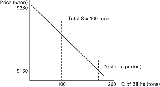
FIGURE 10.1 Annual Demand and Total Supply of Billite
Any principles of economics textbook will tell you that perfectly competitive firms will produce where price equals marginal cost. When price exceeds marginal cost, a firm can increase profit by increasing production. But trying to boost production so that price equals marginal cost, which here is assumed to be 0, would require selling 260 units of stock in a period. But there are only 100 units in total, so this isn’t possible. Even with competitive firms, price will not be driven down to marginal cost, and firms that own stocks of Billite will earn some profit. This profit arises because the resource is scarce relative to demand, and so—as we discussed back in Chapter 3—we call this profit a resource rent.1
Back to the puzzle. How much Billite will be produced and sold in period 1, and how much will be produced and sold in period 2? First, recognize that firms will produce and sell all of their Billite at some point because doing so generates profit and leaving it unsold does not. Therefore, we know that total sales over the two periods will equal the amount of stock: (or ). Because producers face downward-sloping demand, it seems reasonable to think that they will divide the stock evenly between the two periods. That way they sell 50 units in each period and receive a price of $210 for each unit (; ; ).
However, this is not the profit-maximizing outcome. A firm that sells one unit in period 1 and invests the proceeds will have $231 by the end of period . This is better than waiting to sell the unit in period 2 and only getting $210, so there will be pressure to sell more in period 1 and less in period 2. Stated another way, the present value of the sale of a unit of Billite in period 1 is $210 while the present value of the sale of a unit of Billite in period 2 is only . This pressure to sell more in the first period and less in the second period will cease only when firms earn the same amount regardless of whether they sell in period 1 or 2. This occurs where the period 1 price, , and the discounted period 2 price, , are equalized:
With a small bit of algebra, we can rearrange this expression to have prices on one side and the interest rate in the other:
This is Hotelling’s rule, which states that the percentage increase in the resource price will equal the interest rate .
We are getting closer to answering our puzzle: how many units sold in each period? We know that it is not 50/50 and that the quantity sold will be greater in the first period (lowering the first period price) and lower in the second period (increasing the second period price). How much higher and lower? One approach would be to guess and check: Try 51/49, 52/48, and see which combination solves Hotelling’s rule and equalizes the discounted prices in each period. Instead, let’s solve for the answer algebraically.
Using Hotelling’s rule and the inverse market demand curve for each period, we can solve for the amount that will be sold in each period:
We can also use the fact that total sales over the two periods will equal the amount of stock: or :
Period 2 quantity will be . So our final quantities that maximize profit across both periods are 60/40. With this distribution, no firm has an incentive to mine and sell more Billite in one period or less in another.
Moving on to prices: Price in period 1 will be . Price in period 2 will be . Note that discounted period 2 price just equals period 1 price .
Figure 10.2 provides a useful way to show the results of this example. In Figure 10.2, the total width of the figure is 100 units, which represents the total amount of Billite available. We measure Billite produced in the first period starting with 0 on the left and increasing by moving to the right. We measure Billite produced in the second period starting with 0 on the right and increasing by moving to the left. By construction, then, any point along the horizontal axis represents a division of the 100 units of Billite produced between periods 1 and 2 .
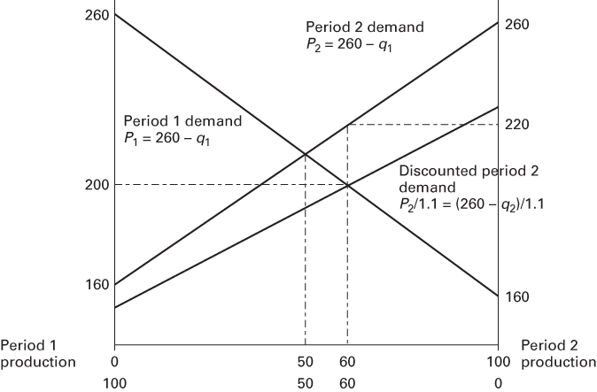
FIGURE 10.2 Resource Use between Two Periods and Hotelling’s Rule
Similarly, we plot the demand for Billite in period 1 (line starting at 260 on the left and sloping downward) and in period 2 (line starting at 260 on the right and sloping upward). Note that without consideration of discounting, the demand curves cross at 50 units produced in each period and at a price of $210 per unit. However, as we noted earlier, what producers really care about is equalizing discounted price: . Discounted period 2 demand is the lower of the upward-sloping lines. As shown, discounted prices are equalized when and so that period 1 price is $200 and period 2 price is $220, which when discounted at 10 percent equals $200.
Figure 10.2 looks almost identical to Figure 4.3 in Chapter 4, which shows the efficient level of pollution reduction. Figure 4.3 shows the marginal benefits of pollution reduction, which is a downward-sloping line showing that it is less beneficial to further reduce pollution, the more pollution has already been cleaned up. Figure 4.3 also shows the marginal cost of pollution reduction, which is an upward-sloping line in pollution reduction showing that it is increasingly expensive to reduce pollution, the more pollution is cleaned up. This diagram is similar. Using more Billite in period 1 generates a marginal benefit to the producers (profit from sale), which is represented by the downward-sloping demand curve in Figure 10.2. However, the more that is used in period 1, the less that can be used in period 2. There is, therefore, a cost of using more Billite in period 1, which is the loss of use in period 2. The marginal cost of increasing period 1 production is thus equal to discounted demand curve in period 2. The efficient amount of production in periods 1 and 2 occurs where , which is where discounted prices are equal: .
This two-period example illustrates a couple of fundamental points. First, as long as the supply of the nonrenewable resource is limited and scarce relative to demand, those who own resource stock will earn a positive resource rent. In the simple example, owning a unit of Billite is worth $200 (in present-value terms). Second, with a positive interest rate, the price of the nonrenewable resource will increase through time. Hotelling’s rule says that the rate of return on the resource, which is the percentage increase in price, is equal to the rate of return on an alternative investment, which is the interest rate. An increase in price is how a positive rate of return for holding the resource stock is generated. Third, if demand is constant across periods, as was assumed in this simple example, then a rising price means falling consumption through time. Here, more was produced and sold in period 1 (60) than in period 2 (40). The higher the discount rate, the more attractive the forgone alternative investments, the faster the stock will be depleted, and the faster the price will rise. Steadily rising prices are the trigger for firms to invest in potential substitutes.
Following Hotelling’s rule is also dynamically efficient. Dynamic efficiency is achieved when the resource stock is allocated over time in a way that maximizes the present value of its use. When discounted prices across periods are equal, there is no way to reallocate sales between periods and increase returns. This result should, perhaps, not be surprising given that the market is competitive and producers have perfect information. However, there often is the feeling that the market outcome is causing resources to be depleted too quickly. Such a conclusion will occur if there is pollution associated with resource use. Then, just as we showed before, there will be too much of the activity associated with pollution generation (and this is a real concern with the use of oil and other fossil fuels that are associated with greenhouse gas emissions and climate change, as well as local air pollution). But without a pollution externality or other distortions, the market will efficiently allocate nonrenewable resources across time.
The basic Hotelling model can be extended far beyond the simple example shown so far, with just two periods and no cost of production. Suppose that the nonrenewable resource can be produced at a constant marginal cost of per unit. The resource rent from production and sales of the nonrenewable resource in this case is price minus marginal cost: . What firms care about is the rent, not just the price. At market equilibrium (where firms do not shift production from one period to another), the discounted resource rent will be equated across time:
So, for example, suppose that in the case of Billite, the marginal cost of production was $42 per unit. In this case, discounted marginal rents will be equalized when
With a higher cost than before, the amount of first-period production falls and second-period production increases. One way to think about why this occurs is that discounting means that firms want to push costs into the future, and this delays production somewhat. In general, an increase in cost, or a fall in demand, will cause resource rent to decline. Lower resource rents tend to lead toward more equal distribution of production over time.
The basic Hotelling logic holds for a model with a large number of time periods. With constant marginal costs of production, in any period in which the resource is produced and sold, the discounted rent (price – marginal cost) is equalized across all time periods.
The resulting prices and quantity produced through time are shown in Figure 10.3 for the case where the demand curve at time is , and there is constant marginal cost of production of per unit. When price rises to the choke price (a), then quantity demanded falls to zero (demand is choked off). This occurs when the resource stock is exhausted at time .
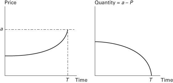
FIGURE 10.3 Hotelling Price and Production Path through Time
As shown in Figure 10.3, there is a time when the resource stock is exhausted (date in the figure). In the run up to date , price is gradually increasing and demand is gradually falling until the choke price is reached, and no one demands the nonrenewable resource anymore. What does this mean in terms of sustainability?
Implicit in this model is that there are substitutes for the nonrenewable resource. As oil becomes increasingly scarce, its price will rise, inducing firms to search out and develop new technologies that serve similar functions at lower cost or that use the existing oil with much greater efficiency. For example, solar, wind, and biomass technologies may power hydrogen fuel-cell or battery-powered vehicles and provide heat and electricity as oil stocks are depleted. Markets can act as one powerful social mechanism for replacing one form of natural capital with other forms of capital. Consumer behavior may also shift. There is a shift toward smaller more fuel-efficient cars during periods of high oil prices (and a shift toward monster trucks when prices are low). Driving habits are also sensitive to oil prices. People will take fewer trips and generally drive less when gasoline prices are high.
In fact, if oil prices go too high (approaching the choke price), then oil is likely to be priced out of the market almost entirely. Eventually, solar-powered electric cars would be cheaper than oil if oil prices continue to increase. Solar/battery-powered cars can be thought of as a backstop technology that provides a readily available and renewable substitute for the nonrenewable resource. Having a backstop technology such as solar power would put an upper bound on oil prices.
But aren’t some resources irreplaceable? This question gets us back to the neoclassical/ecological debate in the previous two chapters. Oil is among the most unique nonrenewable resources, with its high energy content and wide variety of uses that do not have readily available low-cost substitutes. A sudden restriction in oil supplies, given our “addiction,” would no doubt cause a large contraction in the economy and a substantial decline in the standards of living, unless we have adequate energy substitutes. This reason is enough for putting large-scale research and development efforts into developing alternative renewable energy supplies. But before oil literally runs out, Hotelling’s model predicts that price will begin to rise significantly to reflect its scarcity. The price increase will trigger a more serious search for substitutes. And if price gets too high, oil may price itself out of the market as consumers find cheaper alternatives.
Can we rely on the predictions of rising resource prices from the Hotelling model to alert us to looming shortages? We now turn to the empirical evidence on nonrenewable resources.
10.2 Testing the Nonrenewable Resource Model
Do nonrenewable resource prices tend to rise and quantities tend to fall as suggested by the Hotelling model? Throughout the twentieth century, the real price of natural resources, controlling for inflation, was relatively flat or even somewhat downward trending (recall “The Bet” from Chapter 9 in which the prices of five metals fell quite significantly during the 1980s). A comprehensive study examined the real prices for six minerals (aluminum, copper, lead, nickel, tin, and zinc) for the period from 1967 to 2001 (Krautkraemer 2005). Despite some ups and downs, the overall trend in prices was downward during this period. An earlier study by Barnett and Morse (1963) found declining extraction costs for natural resources, except for timber, which of course is a renewable rather than nonrenewable resource, for the period from 1870 to 1958. Until quite recently, natural resources did not seem to be showing signs of greater scarcity as time went on.
Two possible explanations may account for the lack of upward movement in prices of nonrenewable resources through time. First, looking forward at available supply-and-demand conditions, consumers or firms may not have seen long-term shortfalls of these basic commodities within a relevant time frame—say 20 years. So even though there will be scarcity of the resources some time in the future, it is still too far off for it to factor into either consumer or firms’ behavior (Krautkraemer 1998). The second explanation relates to cost reductions. As mining and processing technology steadily advances, lower grade ores can be mined cost-effectively. Technology improvements can expand the amount of the resource that can be produced and reduce scarcity.
A dramatic example of the impacts of new technology on resource availability and prices is the effect of hydraulic fracturing or “fracking.” Fracking is a process by which water is injected under high pressure to open small fractures in the underlying rock formations. These fractures allow oil and natural gas to flow more freely. Some types of rock, notably shale, have been known for some time to contain large quantities of oil and natural gas. However, prior to fracking, there was no economic way to recover the oil and natural gas because it was too tightly locked up in the surrounding rock. With the advent of fracking techniques, these oil and gas deposits became commercially viable.
Fracking has led to a boom in production in the United States, particularly for natural gas production and also for oil. Between 2007 and 2011, natural gas production in the United States increased by over 25 percent from 23.5 billion cubic feet in 2006 to 29.8 billion cubic feet in 2012.2 The rapid increase in supply has resulted in dramatic declines in natural gas prices from a high of over $10 per thousand cubic feet in 2008 to less than $2 per thousand cubic feet in April and May of 2012.3 The increased supply and lowered prices have been a boon to U.S. industries and consumers that rely on natural gas. There are, however, concerns about the environmental impacts of fracking, which include the potential for groundwater contamination from both natural gas and injected chemicals used in fracking, pollution of surface waters when wastes are not properly handled, air pollution, emissions of , and increased seismic activity. How to regulate fracking to minimize the environmental harm is the subject of ongoing debates.
Rather than exhibit a smooth upward trajectory in prices as predicted by Hotelling’s rule, resource prices have bounced around sometime going up but other times going down. In the twentieth century, new discoveries of resource stocks and new technologies seemed to more than offset the resource depletion effect. This pattern may continue in the future as sometimes supply seems to exceed demand and other times the reserve is true. Eventually, a finite supply of a resource has to become scarce. But, eventually, it may be a long time off. Hotelling’s insights into nonrenewable resources are right, but it may be that these insights are well ahead of their time. To investigate this further, we take a deeper dive into the world of oil prices and oil production.
10.3 The Roller Coaster Ride of Oil Prices
Hotelling’s rule predicts that prices for a nonrenewable resource, such as oil, should gradually increase through time. Actual oil prices have not followed this pattern.
There was very little drama in the oil markets prior to 1970. As shown in Figure 10.4, the real price of oil (adjusted for inflation) was flat or declining up until 1970. Since 1970, however, there has been quite a bit of drama with some very large jumps and some very large collapses in oil prices. These rapid price changes have more to do with short-term supply-and-demand imbalances than they do with being signals of long-term resource scarcity.
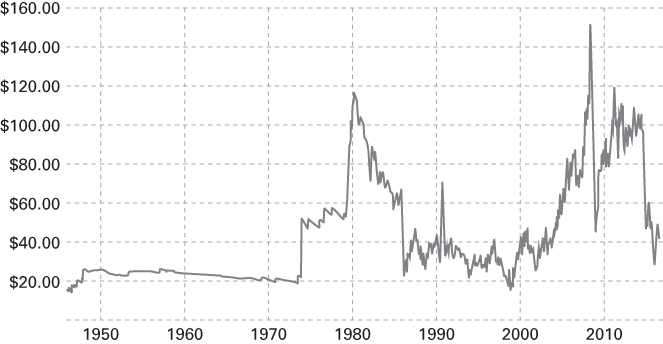
FIGURE 10.4 Oil Prices: Monthly West Texas Intermediate Crude Oil Price 1946– 2016 (2016 constant dollars)
Source: Author’s calculations from EIA oil price data and BLS Consumer Price Index.
In 1973 and 1974, the OPEC oil cartel used its monopoly power to threaten supply reductions and dramatically increase prices. Prices remained at the new higher level throughout the remainder of the 1970s. Then in 1979 and 1980, the Iranian Revolution and the Iran–Iraq war caused a sudden reduction in supply, and prices again rose dramatically. The cumulative effect of price increases, however, set in motion the responses that would cause price to collapse later in the 1980s. High prices lowered demand as consumers switched to more fuel-efficient vehicles and adopted other energy conservation measures. Recession, brought about in part by high prices, further dampened demand. And oil producers outside of OPEC spurred on by high price stepped up efforts to expand production. By the late 1980s, supply shortages had turned to supply gluts, and prices tumbled. Prices remained much lower than they had been throughout the 1990s. But, lower prices led consumers to become complacent, and energy demand increased. Economic growth, particularly in China and other emerging economies, further increased demand. Producers did not have as much incentive to explore and bring new production on line, and supplies did not expand to match increased demand. This set the stage for another rapid rise in oil prices. Oil prices spiked to over $100 per barrel in 2008, quickly collapsed, and then rose again to over $100 per barrel. But, similarly to what happened following the dramatic price increases in the 1970s and 1980s, increase in prices set in motion changes in supply and demand that led to a price collapse that began in 2014. From June 2014 to January 2015, oil price fell from nearly $100 per barrel to below $50 per barrel. Oil prices sank below $30 briefly in early 2016.
Building a roller coaster using oil price data would make for a thrill-packed ride (one that the authors of this book would definitely not take voluntarily). Why have oil prices been subject to such dramatic changes? A major reason for this is the slow adjustment process in production and consumption that makes both supply and demand response sluggish. It takes years from the time an oil company begins exploration and drills new oil wells to when any newly produced oil can finally get to the market. While consumers can change some behavior in the short run (e.g., change the amount of driving on weekends), it generally takes more time to make more fundamental changes such as buying a new car or changing the commute to work. With sluggish responses on both supply and demand, a shock to either supply or demand can send prices skyrocketing or plummeting in the near term. It takes time for supply and demand to adjust to new conditions. And, sometimes, the adjustments overshoot, causing the opposite reaction with regard to prices.
This section has emphasized short-term supply and demand considerations in explaining oil price history. Does the fact that oil is a finite resource play into this at all? Certainly, at some point, it will. Eventually, the limited supply of oil will cause oil prices to rise to reflect scarcity. But when? We now turn to this by considering when oil production might peak and begin to fall.
10.4 Peak Oil?
In 1956, M. King Hubbert, a geoscientist working for Shell Oil, presented a paper at a meeting of the American Petroleum Institute predicting that production of oil in the continental United States would peak in the late 1960s or early 1970s. Starting with Hubbert, a number of analysts have tried to predict the time of peak oil, when oil production hits its high and starts to decline. At the time Hubbert first made his prediction about peak oil in the United States, many in the oil industry thought this was nonsense. At that time production was steadily climbing, many thought it would continue to climb for a long time. In fact, though, U.S. oil production peaked in 1970 at 9.6 million barrels per day. It declined from the peak through the next 38 years, reaching a low of 5 million barrels per day in 2008. It looked as if Hubbert had nailed it. But then, the fracking revolution kicked in. Between 2008 and 2015, production climbed back, reaching 9.4 million barrels per day in 2015. The rise led some analysts to predict even higher production levels in the future. The International Energy Agency predicted that surging oil production would make the United States the largest oil producer, overtaking Saudi Arabia, and make the U.S. energy independent by 2030.4 However, the United States may already have reached a second peak as recent low oil prices have caused oil companies to scale back new drilling and production from existing field declines. U.S. oil production in 2016 showed significant declines from the levels in 2015.
In 1974, Hubbert also predicted that world oil production would peak in 1995. In fact, world oil production has continued to increase (Figure 10.5) and was over 95 million barrels per day in 2015. Some analysts think that increases will continue. The International Energy Agency predicts production growing to over 100 million barrels per day and remaining there through 2040. Others, however, think that peak production will happen much sooner. In a 2008 press release, Royal Dutch Shell, one of the world’s largest oil companies, stated that world demand for oil and gas will outstrip supply within 7 years (i.e., by 2015).5
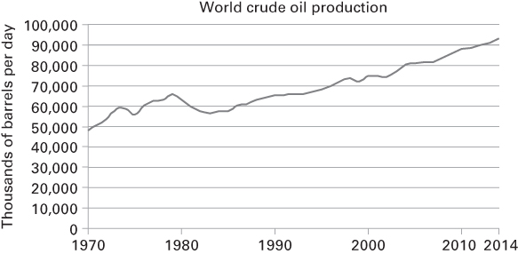
FIGURE 10.5 Peak Oil: Are We There Yet?
Source: US EIA, International Energy Statistics, http://www.eia.gov/cfapps/ipdbproject/IEDIndex3.cfm?tid=5&pid=53&aid=1.
In fact, by 2015, the high oil prices between 2008 and 2014 led to conditions of excess supply of oil in 2015, leading to depressed prices.
At some point, rising demand will run into the physical reality of limited supply. So, in some sense, peak oil shouldn’t be controversial. The real question: when it will occur? Will it be in the next few years, as the Shell oil press release stated, or will oil production continue to climb for several more decades as predicted by the International Energy Agency?
No one knows exactly when peak oil will occur; however, sometime over the next several decades oil production is likely to peak. What will this mean for energy use and energy prices? That depends a lot on energy and climate change policy and on the availability of substitutes for oil. Consider two scenarios for future energy supply. One scenario is that the world remains “addicted to oil,” in which case, resource constraints on oil supply matched with growing demand for energy will lead to very high oil prices. A second scenario is that we will see a shift from oil and other fossil fuels to renewable energy sources. Over the past few years, the prices for wind and solar energy have fallen dramatically, making it conceivable that renewable sources can outcompete fossil-fuel sources to provide the bulk of energy demand going forward. For example, in Denmark and Germany, high electricity prices and an aggressive government tax credit program have led to the explosive growth of wind and solar power production, now serving upward of 20 percent of the countries’ total needs. This clean electricity infrastructure could form the foundation of a system to sustainably replace oil for transportation. (See Sharman 2005.) In addition, concerns over climate change may require that we leave much of the remaining fossil-fuel supply in the ground unused. This is particularly true for coal but may also be true for some oil reserves, such as some of the tar sands in Canada. Climate change may cause us to rethink what is the ultimate constraining resource, which may well be the ability of the atmosphere to absorb greenhouse gases rather than the supply of fossil fuels in the ground.
We will take a much closer look at energy policy in Chapter 18. For now, this tour of the Hotelling model provides a basic understanding of the economics of nonrenewable and how markets with good information should signal scarcity.
When it does occur, peak production will take place against a backdrop of ever-rising demand. With stagnant or declining production, oil prices must rise. At the peak, the world will not have “run out of oil”; we will, however, run out of cheap new oil. In fact, we may have seen the first real signs of this over the past few years. Oil prices have shot up over the past few years (Figure 10.4). They have remained at or above $100 per barrel for several years, far above the historical average price.
Until very recently, however, there was little evidence that oil prices have reflected any long-run scarcity. As shown in Figure 10.4, the real price of oil was flat throughout much of the twentieth century. The figure reveals several big jumps in oil prices resulting from political economic events. In the mid-1970s and early 1980s, the OPEC oil cartel used its monopoly power to increase price; and in 1990, the Gulf War created great uncertainty about short-run oil supplies. The early OPEC price increases did have their predicted impact on energy use. Overall oil consumption in developed nations declined dramatically during the early 1980s as firms and consumers adopted efficiency measures, but after 1985, consumption rose again. However, the oil price run-up that began in 2002, following the war in Iraq and fueled by two decades of explosive growth in China and India, eventually sent prices to their highest level ever. With the onset of the global recession in 2008, prices fell, along with demand—though perhaps tellingly, not back to their early 2000 levels. And as the global economy has recovered, oil prices have climbed again.
No one knows exactly when peak oil will occur; however, sometime in the next 5 to 30 years, production is very likely to peak, and oil prices may rise substantially over where they are today. It may well be that the large and easy deposits of oil have already been found and exploited. Firms will have to drill deeper, in more remote areas, go further offshore into deeper water, or tap smaller, less productive fields. Producing oil in these conditions is more expensive. Petroleum products can also be derived from more abundant but highly polluting and more expensive sources such as tar sands, shale, and coal.
Let us pause to summarize. Hotelling predicted that markets will signal scarcity through prices that rise steadily at a rate more or less equal to interest rates in the economy. Despite their fundamentally limited supply, this has not been true of oil prices, until recently. One critical reason is that very few market participants have good information about the true size of total global petroleum reserves. We also don’t know what breakthroughs in energy technology may occur 5, 20, or 50 years from now that would vastly change the outlook for oil. As a result, Peak Oil might happen soon with very little warning, with rapidly rising prices, and with potentially crippling economic impacts, or it might happen well in the future with a steady run-up in prices, incentivizing new technology, and making the transition manageable. There is no way to know for sure.
Ignoring the major environmental impact of oil production and consumption, are we penalizing future generations by depriving them of a supply of cheap oil? Until 2002, as there had been no long-run upswing in prices, private investors in the United States were not investing heavily in energy technology. That has begun to change with the increase in prices. However, in many other countries where, due to taxes, oil and gasoline prices are much higher, market forces are working more successfully to promote the development of substitute technologies. For example, in Denmark and Germany, high electricity prices and an aggressive government tax credit program have led to the explosive growth of wind and solar power production, now serving upward of 20 percent of the countries’ total needs. This clean electricity infrastructure could form the foundation of a system to sustainably replace oil for transportation. (See Sharman 2005.)
However, oil use in the United States is unsustainable, because both prices and government R&D funding levels are too low to encourage sufficiently rapid deployment of substitutes. Given this, the ecological economists argue that future generations will be penalized in the form of higher prices for transportation and petrochemical products such as plastics. (More significantly, fossil-fuel combustion poses long-term threats to the resilience of the regional and global ecosystems in the form of urban air and water pollution and global warming.)6
10.5 Renewable Resources
Many important natural resources are renewable resources whose supplies are not fixed but grow (“renew”) over time. Fish in the ocean, game species, and forests are biological resources that regenerate and grow, as long as they are not harvested to extinction. Even water supplies are renewable because rain and snow replenish supplies. Similarly, solar and wind energy are renewable as long as the sun shines and wind blows. Unlike nonrenewable resources such as oil or metals, renewable resources can be harvested and used in a sustainable manner. A sustainable harvest is one that does not exceed natural growth so that the renewable resource stock increases or remains the same.
In this section, we concentrate on biological resources such as fish, timber, and game species. We use a growth function to express how much regeneration there is for the resource stock. For example, if currently there are 100 fish and in the next period there will be 120 fish, we would say that growth is 20 fish. Typically, the growth of the resource stock depends on the current size of the stock. For example, as the number of fish increase there are fewer food resources to go around and the birth rate and survival rate of the fish decline. This common feature of growth functions for biological resources is known as density-dependent growth.
An example of a density-dependent growth function for a fishery is shown in Figure 10.6. (A similar function might apply to forests or livestock.) The axis shows the size of the original stock. (Total Fish at the start of a given period.) The axis shows the growth in the stock (New Fish in the next period) as a function of the original stock. The growth function shown in Figure 10.6 reaches a maximum at the stock level labeled , where MSY stands for maximum sustainable yield. Growth falls to zero when the resource stock rises to carrying capacity, . At this point, competition for food and other resources reduces the birth rate to the level of the death rate. Growth is also zero when there is no resource stock (fish that are extinct do not reproduce!).
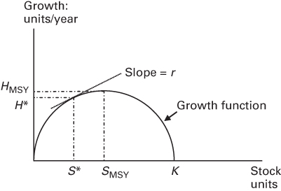
FIGURE 10.6 Growth Function, Maximum Sustainable Yield, and Optimal Harvest
When the resource stock is at , harvest could be set at maximum sustainable yield, shown as (harvesting all the growth in the stock each year) in Figure 10.6. Maximum sustainable yield, , is just equal to the natural growth in the stock and so the stock size will remain at if that number of fish is harvested each year. Managing the renewable resource stock in this way in fact maximizes the amount of harvest that can be done in a sustainable manner.
But will renewable resources be harvested in this manner? No, if firms seek to maximize profits. We will show that profit-maximizing firms sometimes reduce stock below .
To understand the questions about the rate of harvest of renewable resource in a market economy, we need to consider the incentives of resource users. Just as in the Hotelling model for nonrenewable resources, a renewable resource harvesting firm should think about the resource stock as an investment. Unlike oil in the ground, however, fish left in the ocean or trees left in the forest grow and this will factor into the resource firm’s decision about how much to harvest. The growth of the resource means that saving the resource stock will offer a positive return even when the price is not increasing. If the growth of the resource is fast enough, it will make holding onto the resource more valuable than harvesting it right away. However, if the resource growth is too slow, it may be more profitable to harvest everything right now.
To provide more detail on how much competitive firms would harvest and how much of the resource stock would be conserved, let’s return to the country of Billsville. Along the coast of Billsville there are numerous mudflats with a species of clam. Suppose that each portion of each mudflat is owned by an individual clam-harvesting firm. That firm gets to decide how many clams to harvest in period 1 and how many clams to harvest in period 2.
Clams left in the mudflat at the end of period 1 grow in size and reproduce. Let represent the growth function of clams, which depends on the current number of clams . As in Figure 10.6, assume that the growth function (G(S)) starts out with a steep positive slope, but that the slope becomes smaller as the size of the existing clam population increases. We can define marginal growth (MG) as the change in growth with increases in stock or simply as the slope of the growth function. At the maximum sustained yield stock level (SMSY), the marginal growth is zero (slope is zero). For stock levels above SMSY, marginal growth is negative. In this range, growth is actually less with higher levels of stock. As stock increases, growth falls back to zero, and once stock levels hit carrying capacity, K, growth simply stops.
To summarize, the growth of the stock starts at zero, increases until it reaches a maximum at SMSY, and then declines until it becomes zero at carrying capacity, K. Marginal growth (the slope of the growth function) starts out high, falls to zero at SMSY, and becomes negative for stock levels above SMSY.
Suppose that the stock of clams for an individual firm at the beginning of period 1 is and the first period harvest is . This means that clams remain after harvest. It is the remaining clams that can grow and reproduce for the second period. The number of clams at the beginning of period 2 after growth has occurred is equal to :
As period 2 is the last period, the firm will sell all remaining clams in period 2: . Suppose that it costs per unit to harvest clams, the price of clams in periods 1 and 2 is and , respectively, and the interest rate is . By harvesting a unit of clams in period 1, the firm can earn profits off that unit of :
On the other hand, by saving that same unit of clams and letting it grow, the firm will have 1 + MG units of clams in period 2.7 The value to the firm of saving a unit of clams from period 1 and harvesting the additional clams in period 2 is equal to:
Of course, if the firm waits to sell clams until period 2, it must discount the value to get the present value. Just as in the Hotelling model, if , the firm will wish to harvest all its clams now. On the other hand, if , the firm will save all of its clams and harvest them in period 2. In equilibrium, however, the discounted returns will be equal, so setting the two equal allows us to derive the equivalent of Hotelling’s rule for renewable resources:
As noted earlier, renewable resource prices do not have to be rising to ensure that some stock is preserved over time. Even with constant prices there is still an incentive to conserve some of the stock because of its growth. Suppose that prices are indeed constant: . When , then . Using this fact in the previous equation and canceling out terms, we find that equilibrium occurs when , or simply . This relation is known as the golden rule of growth.
The golden rule tells the resource manager to keep increasing the harvest until the growth rate of the stock (MG) is driven down to . Or if the harvest is so high that the growth rate (MG) is less than , the golden rule tells the manager to cut back on the harvest and allow stock to increase, until MG equals . In equilibrium, the returns to investment in the resource must be equal to the rate of return elsewhere in the economy to achieve dynamic efficiency. For renewable resources with constant prices, the return on investment for the resource is equal to the marginal growth. The return on investment elsewhere in the economy is simply the interest rate, .
Returning to Figure 10.6, the golden rule of growth is satisfied when stock is . At this level of stock, , which is shown by noting that the slope of the growth function at equals the interest rate, . The rule characterizing how much to harvest and how much stock to conserve holds with multiple periods as well. In each and every period, the profit-maximizing firm should conserve units of clams and harvest *, which is the natural growth of the clams at .
Finally, note that this is a sustainable harvest because it maintains a constant population of clams at . In other words, if you harvest at a rate *, you are taking away exactly all the growth of the stock generated from : so year after year, assuming no shocks to the system, the population will neither shrink nor grow.
Let’s pause to summarize: So far we’ve talked about harvests that generate the maximum sustained yield and the profit-maximizing yield. If interest rates are positive, note that the model predicts that the profit-maximizing yield will be less than the sustained yield. Why?
Time for a
This puzzle shows that discounting was the key factor explaining the difference between the maximum sustained yield and the harvest satisfying the golden rule of growth that maximized the present value of returns. Indeed, if the discount rate were zero, then the golden rule of growth harvest and the maximum sustained yield would be identical. Both rules would set the resource stock at the point of maximum growth (this can be seen in Figure 10.6) as the point at which the slope of the growth function is zero (i.e., where .
But what about the other extreme? What if the discount rate is really high or the resource is very slow growing? In 1973, mathematical biologist Colin Clark wrote a paper entitled “Profit Maximization and Extinction of Animal Species” (Clark 1973). In this article, Clark showed that for very slow growing species, or very impatient harvesters, the profit-maximizing solution was to harvest the stock to zero—to deliberately cause extinction! The logic of this unsavory outcome is quite straightforward. The resource-harvesting firm earns more money by harvesting the resource and investing the money in higher yield alternative assets rather than conserving the slow-growing (low-return) species. Clark’s main point here was NOT to advocate for harvesting to extinction. He was showing the inexorable logic of profit maximization and what it might mean for species.8
Several important factors might prevent such a dire outcome from ever occurring. First, as a species gets rarer and harvests decline, its price will tend to rise (remember scarcity rent discussed earlier). The anticipation of future high prices might be enough to get some resource stock owners to conserve. Second, species often have value independent of harvest. Most people like panda bears and giraffes and place great value on their existence even though they have no harvest value. Many species have existence value, which is literally a value that people have for the continued existence of the species. If existence value is high enough and resource owners can be paid for existence value, it will never be profit maximizing to cause extinction. Generally speaking, private owners of renewable and nonrenewable resources are incentivized to engage in some level of profit-based conservation and not immediately liquidate the resources they own.
Extinction pressure may come through another route—open-access resource harvesting that leads to “the tragedy of the commons” (see Chapter 3). Suppose that instead of clams, Billsville was famous for “Billfish” that swim in the ocean off the coast. And suppose that anyone who wants to can go and catch fish. As long as there is a profit from catching fish, someone will go and catch more fish. There is no incentive for any individual fisherman (or fisherwoman) to conserve the fish stock because someone else will catch the fish. In the case of open access, it is as if there was an infinitely high discount rate because no individual can afford to think about the future. As long as it remains possible to profitably harvest a species even as it gets very rare, then the species will be hunted or fished to extinction.
10.6 Renewable Resource Policy: Fisheries and Endangered Species
As discussed in Chapter 3, the solution for the tragedy of the commons is to set some type of limit on harvest. Fisheries with functioning quota systems that limit harvests have generally been successful at sustainable management while those that have not generally seen overfishing and large declines in stock abundance (see Costello, Gaines, and Lynham 2008).
The standard regulatory recommendation for fisheries management from economists is a form of a cap-and-trade system called an individual transferable quota or ITQ. (For more on the generic pros and cons of marketable permits, see Chapters 15 and 16.) The basic idea is that a regulatory agency sets a total allowable catch (TAC), preferably at the efficient level, but definitely at or below maximum sustained yield. Then each firm receives a permits allowing it to harvest a certain percentage of the TAC, equivalent to a specified tonnage of fish. These permits can be bought and sold, but at the end of the season, a firm needs to be in possession of enough permits to cover its harvest, or else pay a stiff fine.
How are ITQs distributed? They can be auctioned by the government, or they can be given away to existing fishing firms on a “grandfathered” basis; that is, firms receive an allocation based on catch history.
The advantage of ITQs over rigid allowances is the flexibility built into the system. If a boat is having a particularly good season, the owner can purchase or lease additional quota from vessels not having as much luck. And over the long run, more efficient operators can buy out less efficient operators. Some have criticized ITQ for this kind of impact. ITQ systems encourage the departure of small operators, leaving more efficient boats (sometimes giant factory trawlers) a larger share of the market. While this may lead to a lower cost industry, it also leads to consolidation in an industry traditionally hosting small, independent producers.
A variety of practical problems are inherent in the implementation of any kind of fisheries regulation, including ITQs. Generic problems include political influence over regulators, leading to excessive TAC levels and difficulty monitoring mobile sources such as fishing boats. The so-called bycatch—fish accidentally caught for which boats don’t have permits—is also a problem. Bycatch is often dumped overboard to avoid fines—a wasteful process. New Zealand has been our major laboratory for ITQs; most of the nation’s fisheries have adopted the system. The results have been generally positive. While some small fishers have exited, they were the unprofitable ones to begin with.
Researchers have found that “the industry started out with a few big players (especially vertically integrated catch and food processing companies) and many small fishing enterprises, and it looks much the same today. The size of holdings of the larger companies, however, has increased.” In other words, small producers generally managed to survive, but big producers have gotten bigger. Fish populations have either stabilized or improved under the ITQ system, and fishers have altered their practices to avoid bycatch and stay below permitted levels. And finally, the total value produced by the fishery more than doubled between 1990 and 2000.9
ITQ systems are one way to overcome the open-access problem. A second way is to assign individual property rights in ocean resources to fish farmers. Aquaculture—the commercial raising and harvesting of fish in ocean environments over which fishers are granted exclusive rights—is an old industry with its roots in oyster farming. But in recent years the industry has expanded into freshwater species such as catfish and tilapia and ocean-raised salmon and shrimp. Globally, aquaculture has undergone dramatic growth so that by 2010, it was four to five times as large as it had been in 1990. Aquaculture currently supplies half of the fish consumed globally (FAO 2013).
Aquaculture has the potential to significantly decrease pressure on natural fisheries as well as boost the productivity of the oceans. However, as currently being practiced, aquaculture generates significant negative externalities, including the impact on the immediate ocean environment from fish waste, heavy metals, pesticides, and antibiotics. In addition, fish feed for the carnivorous species such as salmon is often harvested unsustainably in the open ocean; approximately one-third of the world’s total annual ocean catch is currently used for fish food! And finally, aquaculture can destroy local habitats. For example, many of Thailand’s mangrove swamps—shoreline stabilizers—have been cut down and converted to shrimp farms.10
In a world likely to be inhabited by more than half as many people by 2050, our ocean commons need to be maintained as an important source of both food and biodiversity. Effectively managing and restoring fisheries is a critical task. Some combination of ITQ management for open-ocean fisheries (combined with regulations protecting habitat) and sustainable aquaculture must provide the answers.
One point worth stressing is that there is large uncertainty about the likely future level of many resource stocks. The populations of many species are subject to great variability. Disease outbreaks or unfavorable weather (drought, flood, and extreme cold or heat) can result in sudden large population reductions. Even seemingly minor environmental changes have led to large changes. Fish populations in particular are subject to high year-to-year variability in “recruitment,” the number of fish born that survive to maturity. Trying to maintain a steady harvest policy, such as maximum sustained yield or the golden rule of growth harvest, in the face of highly variable populations is likely to lead to trouble. For example, suppose that unfavorable environmental conditions lead to growth being reduced by 50 percent. Keeping Maintaining harvest at maximum sustained yield set under normal circumstances will result in harvests that greatly exceed natural growth. The stock level will then fall. With lower stock, growth will be reduced. If harvest levels are maintained, this will cause further stock declines leading to a vicious downward spiral.
Highly variable resource stocks should cause resource managers to continually adjust harvest levels to try to maintain stocks at desired levels. In fact, some work on fisheries with variable recruitment has shown that the optimal management policy is to aim for a constant population size in which harvests expand in good years and contract in poor years to match growth.11 But this places a lot of burden on getting accurate information and often puts managers at odds with harvesters who don’t want to be told to cut back on harvests. And there is often political pressure to keep harvest rates up even when there is evidence that the stock is falling, which intensifies the problem of declining resources.12
When future conditions are highly uncertain, it is often not possible to make decisions about harvest rates and conservation in the same way as when there is certainty about what the future holds. For example, if fish harvesting quotas are set assuming an average year but it turns out to be a very poor year, the quota may greatly exceed what is sustainable. This fact has led some economists to advocate what is called a safe minimum standard (SMS) for threatened resources. SMS advocates argue that unique resources should be preserved at levels that prevent their irreversible depletion, unless the costs of doing so are “unacceptably” high.13 The SMS is thus another version of the precautionary principle discussed in Chapter 8. In a fisheries context, the SMS sometimes takes the form of setting aside Marine Protected Areas, which prohibit fishing within it to allow for continued conservation of marine species.
Figure 10.8 illustrates the basic idea behind the SMS. The horizontal axis shows the current stock of a renewable resource, in this case, mating pairs of spotted owls in a forested area. The S-shaped line relates the stock of owls alive today to the stock of owls around next year, graphed on the vertical axis. So, for example, if there are seven pairs alive this year, there will be five pairs alive next year, thus implying that the natural death rate exceeds the birth rate. Carrying this logic further, if there are 5 pairs next year, there will be only 2.5 pairs the year after that, and so on, to extinction. Points on the 45-degree line reflect stable populations, because the number of owls in the next period is the same as that in current period.
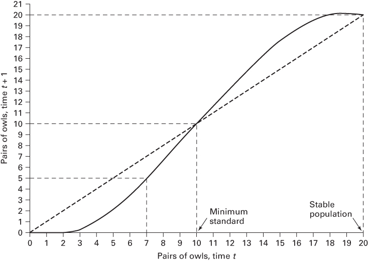
FIGURE 10.8 The Safe Minimum Standard
The point where the S curve first crosses the 45-degree line (10 pairs) is called the minimum standard (MS); any fewer owl pairs than the MS, and the species begins to decline in numbers, eventually slipping into extinction. With more pairs than the MS, however, the species will recover, as a given stock this period produces a larger stock next period, and so on. Eventually, the population size will stabilize at 20 pairs. (Extra credit question: Why does the S curve bend back down and not keep rising?)
The SMS lies somewhere to the right of the MS—say 12 or 14 pairs—at the point where the resource can be guaranteed to recover on its own. Getting too close to MS would allow some bad outcome to push the spotted owl below MS and put the owl on the road to extinction.
The SMS argument is often applied to endangered species. Each species has highly unique biological properties as well as uncertain future genetic value; and Jurassic Park aside, species extinction is irreversible. Moreover, endangered species often serve as indicator species for threatened ecosystems. Thus, saving the spotted owl in the Pacific Northwest means saving a complex and biodiverse old-growth forest ecosystem. Especially considering their role as indicators, endangered species clearly merit protection under a precautionary principle approach.
In fact, as we noted in the previous chapter and will explore further in Chapter 13, endangered species legislation is the one major national law currently on the books that reflects ecological sustainability as an underlying goal. The law states that natural capital in the form of species must be protected from extinction, regardless of the cost.
10.7 Ecosystem Services and Natural Capital
Economic analysis of renewable and nonrenewable resources focuses on the rate of use of particular resource stocks. This type of analysis is clearly relevant for such things as fish harvested commercially, oil lifted from the ground, or metals mined. But the ways in which the natural world contributes to human well-being are much broader than just the supply of these resources. Ecosystem processes filter pollution, pollinate crops, regulate climate, improve soil fertility, and provide numerous other ecosystem services on which human well-being depends. In this section, we consider the much broader issue of managing ecosystems to supply a wide range of ecosystem services rather than managing for one specific resource.
Ecosystem management differs from specific resource management for three main reasons: joint production, unintended consequences, and the importance of spatial analysis.
Ecosystem management involves joint production of multiple ecosystem services. For example, a forest not only produces timber but also provides habitat for game species, stores carbon to reduce the amount of in the atmosphere, filters air and water pollutants, and prevents soil erosion. There often are important trade-offs among ecosystem services.
Ecosystems are complex, interconnected systems. Ecosystem management directed toward one objective, such as increasing timber production, can cause unintended consequences for the provision of other ecosystem services, such as the loss of habitat for forest-dwelling species. Minimizing the unintended consequences of management actions requires first understanding how ecosystems function. How might cutting trees for timber in a particular location affect the ecological process in the forest? For example, will timber harvests lead to increased soil erosion that will cause buildup of silt in nearby streams that can affect fish and other aquatic life? Gaining this type of understanding is primarily a question for environmental scientists.
But minimizing unintended consequences also requires providing incentives so that decision-makers, be they private landowners, firms, or government agencies, take proper account of the consequences on the multiple ecosystem services affected by their decisions. For example, if cutting trees near streams leads to water quality problems, then there may be a need for either regulation that mandates a buffer along streams or incentives that make it costly to cut trees near streams without taking precautions for water quality concerns. The task of designing regulations or incentives falls in the lap of environmental economists, often working closely with environmental scientists.
Ecosystem management for ecosystem services also puts a premium on spatial analysis. Much of economics ignores where things happen. But for ecosystem services where is often the crucial question. There is great variability in ecosystems because of differences in climate, soil, and other environmental variables so that ecosystem services are only provided in certain locations and not others. Forests grow only where there is adequate moisture and suitable temperatures. Deserts occur in places with little rainfall. The location of ecosystems in relation to the location of people is also an important determinant of the value of ecosystem services. For example, coastal wetlands absorb the energy from waves and reduce the risk of flooding further inland. If coastal wetlands protect towns or cities further inland, the value of coastal protection services will be high. But, if no one lives near the wetland, then there is little value from coastal protection. Some ecosystem services require close proximity of different elements. For example, the ecosystem service of pollination depends on having close proximity of pollinators, which often require natural habitat, and agricultural fields that have crops that need pollination. For all of these reasons, ecosystem management for ecosystem services requires spatial analysis that addresses questions of where things occur.
Analysis of ecosystem services is relatively new in economics. The vast majority of the work by economists on ecosystem services has happened since the publication of the Millennium Ecosystem Assessment in 2005 . One influential article that predated the Millenium Ecosystem Assessment addressed the economic value of conserving intact ecosystems versus the value of extracting resources by transferring the ecosystem (Balmford et al. 2002). The authors compared “reduced impact logging” to “conventional logging” in Malaysia; “reduced impact logging” to “plantation conversion” in the Cameroon; “intact mangrove” ecosystems to shrimp farming in Thailand; “intact wetlands” in Canada to intensively farmed lands; and “sustainable fishing” to “destructive fishing” in coral reef ecosystems in the Philippines. The study included the value from a wide range of services, such as the value of timber harvesting, crop production, fisheries, water supply, hunting and gathering activities, recreation, carbon sequestration, and protection of endangered species. In all of the five cases analyzed, the value of ecosystem services generated by a relatively intact natural ecosystem exceeded the value from heavily modified ecosystems. Plantation forestry in Cameroon actually had negative net benefits (operation costs exceeded the benefits) and was only possible to carry out because of government subsidies.
Making the comparison across alternative ecosystem management requires knowing the level of service provision for each ecosystem service under each alternative. Estimates of service provision can be generated by looking at the data for both intact and modified systems or by using ecological production functions. Production functions in economics predict the output of final goods that can be made with a certain amount of inputs (labor, machinery, and raw material). Ecological production functions predict the provision of ecosystem services (output) given the state of the ecosystem (input). Ecological production functions are useful for predicting how ecosystem service provision will change if the ecosystem is altered, either because of climate change, land-use change, or changes in management.
A recent study of ecosystem service provision by Nelson et al. (2009) used ecological production functions combined with economic valuation to show the impact of alternative land-use scenarios on ecosystem service provision in the Willamette Basin in the state of Oregon. The study used a model called InVEST (Integrated Valuation of Ecosystem Services and Trade-offs) to predict how land-use change under three scenarios (business-as-usual, development, and conservation) would affect carbon sequestration, flooding, water quality (phosphorus loadings), erosion, biodiversity conservation, and the combined market value of timber production, agricultural crop production, and housing development.
Applying the InVEST model, Nelson and colleagues quantified the amount of increase in ecosystem services under the conservation scenario compared to the other two scenarios. The conservation scenario preserved more natural areas compared to the other two scenarios and resulted in greater provision of ecosystem services. The only exception to this outcome was that the combined market value from timber, agriculture, and housing was lower under the conservation scenario. If landowners are only paid for market values, they will tend to prefer either the business-as-usual or development scenarios. However, for society as a whole, the value of the other ecosystem services makes the value of the conservation scenario higher than either of the other two scenarios. Nelson and colleagues showed that providing payments even for only one ecosystem service, sequestering carbon, would be enough to make the conservation scenario generate higher value to landowners compared to the other scenarios. In this case, instituting a scheme for carbon payments would provide enough incentive for landowners to conserve more land, which would generate higher payments to landowners and would also be good for species conservation (Figure 10.9).
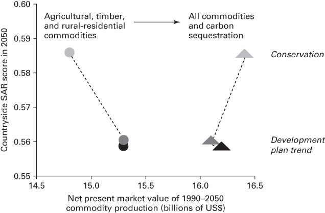
FIGURE 10.9 The value of marketed commodities and biodiversity conservation under the conservation, development, and plan trend (business-as-usual) scenarios. Without paying for ecosystem services there is a trade-off between biodiversity conservation and values for landowners (illustrated by the circles). With payment for carbon, values for landowners and biodiversity conservation are higher under the conservation scenario (illustrated with the triangles).
Source: Nelson et al. (2009)
Many of the benefits generated by more intact ecosystems come from public goods. Private landowners or firms generally do not capture these benefits. Often they are better off converting land to realize private benefits even though this may result in loss of the benefits from public goods. For example, a farmer who drains a wetland to plant crops can generate profit from selling the crops. Protecting the wetland does not generate income for the farmer, even though it provides habitat for ducks and other species, filters nutrients to provide cleaner water downstream, sequesters carbon, and regulates the flow of water. The farmer will typically choose to drain the wetland. Preserving the wetland to provide for public goods requires providing the farmer with incentives to do so.
One direct way to provide such incentives is to institute a program of payment for ecosystem services (PES). In a PES program, landowners who agree to certain land use or management practices that generate ecosystem services are paid for doing so. For example, municipal water supply agencies in Quito, Ecuador, and in New York City have targeted payments to landowners in watershed areas that supply water for these cities. A properly designed PES will result in payments being sufficiently attractive so that the landowners are better off with conservation, and cities are better off because they get clean water more cheaply than having to build expensive water treatment plants to clean up polluted water. New York City was able to forestall the construction of an expensive water filtration system by instituting programs to protect watersheds in the Catskill Mountains that are the source of drinking water for the city. PES expenditures to date—paying farmers to adopt best management practices for livestock and towns and households to upgrade their sewage and septic systems—have been far less than the cost of building and operating a water filtration system.
The values of ecosystem services can be large and, if properly taken into account, could lead to many changes in ecosystem management. There is huge interest at present in finding out how economic decisions affect the provision of ecosystem services and whether society would benefit from greater protection of specific ecosystems. Such information can be important in evaluating the costs and benefits of local or regional projects. Such information is also important in calculating national-level accounts of net national welfare or inclusive wealth (see Chapter 9).
10.8 Summary
This chapter has looked more deeply into the economics of nonrenewable and renewable resources (traditional resource economics) and the much more recent analyses focused on the economic value of ecosystem services. Resource economics provides guidance for firms interested in maximizing profits from the resources they control. And assuming that firms follow that advice, resource economics makes predictions about how firms will conserve, or exploit, resource stocks.
The key to resource economics comes from understanding that holding resources is a form of investment. If nonrenewable prices (or more technically, resource rents) are rising more slowly than the rate of interest, the Hotelling model shows that it makes economic sense for holders of resources to develop more of the stock today instead of holding it for the future. This way, they can make money now and bank the money at a higher rate of interest. This in turn reduces supply in the future and raises prices (and resource rents) in the future. In equilibrium, resource rents will rise at the rate of interest. The reverse logic also holds: persuade yourself what you should do if resource rents are rising more rapidly than the rate of interest.
Following this logic, the Hotelling model concludes that competitive firms should allocate stocks of nonrenewable resources so that prices rise through time. Hotelling’s rule states that the percentage increase in resource rents is equal to the rate of interest. The observed failure of nonrenewable resource prices to rise in much of the twentieth century may reflect either no imminent shortage of resources or improvements in technology that effectively expand the amount of stock that can be economically produced (e.g., the fracking revolution). Oil prices in particular have not followed a Hotelling-like path. Since the 1970s, oil prices have been on a dramatic roller coaster ride with large price increases and decreases. Rapid price movements are caused by shocks to either supply or demand and sluggish responses by producers and consumers.
Concerns about peak oil can thus best be understood as concerns about the failure of the Hotelling model’s predictions to come true. If prices fail to rise steadily well in advance of hitting the peak, then there are no strong market signals driving the development of substitute technologies. In that case, a global economy addicted to oil would suffer through an extended period of painful withdrawal. And indeed, if at that time, clean substitutes for oil are not yet available, it is not clear if a crippled global economic system would then be able to deliver them. Alternatively, prices may signal impending resource scarcity giving producers an incentive to search for substitutes (e.g., renewable energy sources to replace fossil-fuels) and consumers an incentive to reduce energy use.
Similarly to nonrenewable resource markets, conserving renewable resources for future harvest is a form of investment. However, here things are complicated by the fact that renewable resources grow naturally over time. The Golden Rule in this case tells resource managers to shift their harvesting practices (either decreasing or increasing them) so that the marginal growth rate of the resource stock (the change in the growth rate) is just equal to the rate of interest.
High discount rates will drive higher rates of near-term exploitation (and smaller optimal stocks) as firms seek to derive near-term gain and bank those gains. If the interest rate is high enough, or resource growth is slow enough, the cold-blooded, profit-maximizing strategy would be to drive the resource to extinction and invest the profits elsewhere in the economy. Economists do not endorse this idea but point out that this result follows from the logic of profit maximization. If, however, the resource has existence value, then it may be optimal to conserve even slow-growing resources.
In general, in both nonrenewable and renewable markets, resource owners do have some profit-based incentive for conservation, driven either by the prospect of rising prices or by the growth of the underlying resource. Open access—when ownership of resources is not defined—can be thought of as a resource situation with very high discount rates. If one actor restrains from catching fish (or lifting oil or water out of a common underground pool), he or she receives very little benefit in the future, as the catch (or oil or water) will be scooped up by a competitor. Thus, profit-based incentives for conservation are undermined.
In the real world, growth functions for some resources are not typically as well-defined or stable as the inverted U shape we illustrated in Figure 10.6. Fisheries managers, for example, typically set TAC levels to sustain species, not necessarily at profit-maximizing levels. ITQs can improve efficiency and help managers keep their fisheries sustainable. In cases when conditions are highly variable and there is some risk of allowing unsustainable catch, an SMS can be imposed; in the fisheries context this might involve the creation of Marine Protected Areas to support sufficient breeding stock to ensure recovery of the species. The SMS is an application of the precautionary principle.
Finally, economists working with environmental scientists have recently begun to model the complex ecosystem processes that generate ecosystem services. Ecosystem processes typically involve joint production of multiple services. Managing the system for one services, such as timber production, and have unintended consequences on the provision of other services, such as carbon sequestration and preventing erosion that damages fish habitat. In addition, spatial context is important: where things occur matters. The magnitude and types of services generated by an ecosystem vary as a result of differences in underlying geology, hydrology, climate, and mix of species. The value of ecosystem services also depends crucially on where services are generated relative to the demand for those services by people. If a wetland stores water and lowers flood risk but there are no people in the watershed, then the service of flood control has no value.
The previous three chapters have explored the economic impacts of decisions taken today on the well-being of future generations, to assess the underlying goal of sustainability. The goal is easy to understand conceptually—we want to maintain or improve the quality of life for the typical member of generations to come. However, we have seen that putting it into practice requires judgments about the degree to which manufactured, social, and human capital can offset reductions in natural capital in the production of goods and services critical to human well-being. We now leave this conversation and turn to one final debate: what does economic growth really buy us? If we get richer, do we get happier? And if not, then why “pave paradise to put up a parking lot?”
KEY IDEAS IN EACH SECTION
- 10.0 Traditional resource economics focused on nonrenewable and renewable resources. More recent analysis has recognized that natural capital also includes the ecosystem processes that underlie ecosystem services. These services include provisioning, regulating, supporting, and cultural services.
- 10.1 The Hotelling rule illustrates that in competitive markets, a profit-maximizing equilibrium will occur in which the resource rents generated from scarce, nonrenewable resources will rise at the rate of interest. A choke price is defined as the price at which demand falls to zero: the choke price reflects the existence of a backstop technology to which users switch at a given price.
- 10.2 Hotelling predicts that markets will signal scarcity with steadily rising prices, providing incentives and time for firms to invest in substitutes. This was not true for nonrenewable resources until 2000, but since then, prices for most commodities, including oil, have risen. (The exception is natural gas, where new “fracking” technology has unexpectedly increased global reserves.) Prior to 2000, most resource markets were not signaling scarcity, but now appear to be.
- 10.3 Historically, individual oil fields exhibit an inverted U shape for production. Hubbert predicted that the same would be true for regional and global oil supplies. The challenges to assessing the timing of global peak oil include poor information about the size of the existing oil stocks and disagreement about technological change that might make exploitation of currently marginal oil sources economic. As a result, we do not know if peak oil will occur soon and suddenly, causing large-scale disruption, or gradually and manageably.
- 10.4 Renewable resources can be characterized by a growth function relating the growth in a given period to the size of the stock at the beginning of the period. Growth functions sometimes display density-dependent growth. A sustainable harvest is one in which the size of the stock does not decline over time, and the Maximum Sustainable Yield is the largest possible sustainable harvest. For renewable resources, the Golden Rule of Growth tells profit-maximizing managers to adjust their harvests up or down so that the marginal growth rate, MG(S), is equal to the interest rate. If the discount rate is high enough or the growth rate low enough, profit maximization can lead to liquidation of the resource and investment of the resource rents elsewhere. Generally, however, both renewable and nonrenewable resource owners do have incentives for profit-based conservation.
- 10.5 In fisheries, Total Allowable Catch (TAC) levels are set to try and control open access and ensure sustainability of the fishery. Individual Transferable Quotas (ITQs) can reduce the problem of excessive capitalization: too many boats chasing a set number of fish. Aquaculture also helps solve the open-access problem, but has its own environmental challenges. Safe Minimum Standard (SMS) management is used for threatened and endangered species, where stock levels ensuring species recovery are required. SMS is thus an application of the precautionary principle.
- 10.6 Ecosystem services are provided by underlying ecological processes. The flow from processes to services is modeled using an ecological production function. Ecosystems typically produce joint outputs; focusing management attention to optimize the production or harvest of a single output can lead to unintended consequences in terms of reduction in other outputs. Finally, ecological production functions vary across geographies, requiring a focus on spatial analysis. Ecosystem service modeling is quite recent, but the results suggest that the value of intact ecosystems can be higher than the value of individual commodity production that degrades the ecosystem. One way to preserve the services is through payment for ecosystem services (PES) policies.
REFERENCES
- Balmford, Andrew, Aaron Bruner, Philip Cooper, Robert Costanza, Stephen Farber, Rhys E. Green, Martin Jenkins, et al. 2002. Economic reasons for conserving wild nature. Science 297: 950–53.
- Barnett, Harold J., and Chandler Morse. 1963. Scarcity and growth: The economics of natural resource availability. Washington, DC: Johns Hopkins University Press.
- Bishop, Richard C. 1978. Endangered species, irreversibility, and uncertainty: The economics of a safe minimum standard. American Journal of Agricultural Economics 60(1): 10–8.
- Ciriacy-Wantrup, S. V. 1968. Resource conservation: Economics and policies. 3rd ed. Berkeley: University of California Press.
- Clark, Colin. 1973. Profit maximization and the extinction of animal species, Journal of Political Economy 81: 950–61.
- Costello, Christopher, Steven Gaines, and John Lynham. 2008. Can catch shares prevent fisheries collapse? Science 321: 1678–81.
- Costello, Christopher, Stephen Polasky, and Andrew Solow. 2001. Renewable resource management with environmental prediction. Canadian Journal of Economics 34(1): 196–211.
- Daly, Herman. 1996. Beyond growth: The economics of sustainable development. Boston: Beacon Press.
- Food and Agriculture Organization (FOA). 2013. FAOSTAT. Rome: FAO.
- Goldberg, R. J., M. S. Elliot, and R. L. Taylor. 2001. Marine aquaculture in the United States. Arlington, VA: Pew Oceans Commission.
- Hotelling, Harold. 1931. The economics of exhaustible resources. Journal of Political Economy 39: 137–75.
- International Energy Agency (IEA). 2012. World energy outlook 2012. Paris: International Energy Agency.
- Krautkraemer, Jeffrey. 1998. Nonrenewable resource scarcity. Journal of Economic Literature 36(4): 2065–107.
- Krautkraemer, Jeffrey. 2005. Economics of natural resource scarcity: The state of the debate. Discussion paper 05-14. Washington, DC: Resources for the Future.
- Ludwig, Donald, Ray Hilborn, and Carl J. Walters. 1993. Uncertainty, resource exploitation, and conservation: lessons from history. Science 260: 17,36.
- Millennium Ecosystem Assessment. 2005. Living beyond our means: Natural assets and human well-being. Washington, DC: Island Press.
- Nash, Colin, ed. 2001. The net-pen salmon farming industry in the Pacific Northwest. Seattle, WA: Northwest Fisheries Science Center.
- Nelson, Erik, Guillermo Mendoza, James Regetz, Stephen Polasky, Heather Tallis, D. Richard Cameron, Kai M. A. Chan, et al. 2009. Modeling multiple ecosystem services, biodiversity conservation, commodity production, and tradeoffs at landscape scales. Frontiers in Ecology and the Environment 7(1): 4–11.
- Reed, William. 1979. Optimal escapement levels in stochastic and deterministic harvesting models. Journal of Environmental Economics and Management 6: 350–63.
- Sanchirico, James, and Richard Newell. 2003. Catching market efficiencies. Resources 150: 8–11.
- Sharman, Hugh. 2005. Why wind power works for Denmark. Civil Engineering 158: 66–72.
- Shell Oil. 2008. World demand to outstrip supply. Press Release, 25 January. http://royaldutchshellplc.com/2008/01/24/the-times-shellchief-fears-oil-shortage-in-sevenyears/.
- U.S. Energy Information Administration. U.S. Natural Gas Gross Withdrawals. http://www.eia.gov/dnav/ng/hist/n9010us2A.htm.
- U.S. Energy Information Administration. U.S. Natural Gas Wellhead Price. http://www.eia.gov/dnav/ng/hist/n9190us3m.htm.